Evaluation of wind forecasts over Svalbard using the high-resolution Polar WRF with 3DVAR

ABSTRACT

In this study, the performance of wind forecasts over Svalbard, located between the Arctic Ocean and the Norwegian Sea, was evaluated using the Polar Weather Research and Forecasting (PWRF) model and three-dimensional variational data assimilation (DA) system. The forecasts of the analysis–forecast cycling experiment using the PWRF 3DVAR were compared with those of the cold start experiment using reanalysis as the initial condition. Three strong wind cases that occurred during January and February 2011–2012 were selected, where polar lows were generated on the east coast of Greenland and generated a wind speed above 20 m s⁻¹ in Svalbard. The wind speed forecasts for both cycling and cold start experiments were similar to the highest 10-minute average wind speed for the last 1 hour (HAW). The average root mean square error (RMSE) of the forecasts in the cold start experiment from HAW was 3.78 m s⁻¹ for three cases and was greater than that in the cycling experiment. The forecast performance in the cycling experiment was comparable to, or even better than, that in the cold start experiment, which implies that the cycling system with DA is more useful than the cold start system in forecasting polar weather to support research activities.

KEYWORDS:

• Polar WRF with 3DVAR
• data assimilation
• wind forecast
• polar low
• Svalbard

Introduction

Polar lows are generally smaller than synoptic-scale lows at midlatitude but develop more rapidly and strongly. Thus, it is difficult to predict the polar low that causes severe weather conditions with high wind speeds near the surface (Klein and Heinemann 2002). Many studies have been conducted to understand the genesis and development mechanism of the polar low (Grønås and Kvamstø 1995; Tilinina, Gulev, and Bromwich 2014). The genesis of the polar low is affected by several factors such as the instability of the lower atmosphere, upper air flows, and energy exchanges at the surface (Claud, Duchiron, and Terray 2007; Kristjánsson et al. 2011). The condition of polar low generation is usually determined by the instability of the lower atmosphere, whereas the generation time of the polar low is determined by the upper air flows (Kolstad 2011). The baroclinicity increases when the cold air of the lower atmosphere moves over the region of high-temperature gradient near the surface (Rasmussen and Turner 2003). Thus, the polar low typically occurs when the cold air on the sea ice moves to the relatively warm ocean of the Labrador Sea in the southwest of Greenland or the Greenland–Iceland–Norwegian Seas to the east of Greenland. The polar low can be generated and developed abruptly when the negative (positive) anomalies of the 500 hPa geopotential height/temperature (potential vorticity) approach baroclinic regions in the lower atmosphere (Blechschmidt, Bakan, and Graßl 2009).

To predict the rapidly developing polar low accurately, the detailed simulation of synoptic-scale atmospheric flows and terrain effects using the high-resolution numerical weather prediction (NWP) model is necessary (Zappa and Shaffrey 2014; Moore et al. 2015; Smirnova and Golubkin 2017). Because the forecast accuracy of the polar low is sensitive to the model domain, using the appropriate experimental domain is also important (Kristiansen et al. 2011). Adaptive observations in the sensitivity region at the beginning of the polar low genesis would be beneficial for improving forecast accuracy (Jung et al. 2016). Aspelien et al. (2011) and Irvine, Gray, and Methven (2011) showed that the forecast accuracy of the polar low affecting the Scandinavian Peninsula increases as targeted dropsonde observations are added to the region with sparse observations. In addition, using appropriate physics schemes that consider the characteristics of the polar environment in the NWP model is important for enhancing the accuracy of forecasting polar lows.

The Polar Weather Research and Forecasting (PWRF) model used in this study has been developed with a focus on the parameterization of the planetary boundary layer (PBL), microphysics, and the land surface process in the polar region with sea ice. Hines and Bromwich (2008) optimized the Noah land surface model appropriate to the polar environment and applied the effect of the surface snow to the PWRF. Bromwich, Hines, and Bai (2009) considered the effect of fractional sea ice using the mosaic method, and Hines et al. (2015) considered the effect of spatially varying sea ice and snow thicknesses in the PWRF. The validity of optimizing the WRF for the polar region was demonstrated by testing the performance of the PWRF for various polar regions and surface conditions (e.g., ice sheet, polar ocean with sea ice, and arctic land; Bromwich, Hines, and Bai 2009; Hines et al. 2011; Wilson, Bromwich, and Hines 2011). As a result, the PWRF in the Antarctic Mesoscale Prediction System  (AMPS) is used for operational forecasts in the Antarctic (Powers et al. 2012), and the PWRF was used for producing the Arctic System Reanalysis (ASR) data in the Study of Environmental Arctic Change  (SEARCH) program. The ASRv2 data with 15-km horizontal resolution were produced using the PWRF with the three-dimensional variational (3DVAR) data assimilation (DA) system and a High-Resolution Land Data Assimilation System (HRLDAS) (Bromwich et al. 2018).

The high accuracy of the NWP model is required to diagnose and analyze meteorological characteristics in the polar region where few observation data have been obtained. Although Jung et al. (2016) mentioned that the forecasts in the polar region need to be evaluated focusing on the variables (e.g., near-surface wind) that are necessary for weather information users, the performance of the high-resolution PWRF coupled with DA has not been fully evaluated by near-surface observations for specific cases. Most studies on polar lows have been conducted for observation campaigns. Although Svalbard is affected by the high wind caused by polar lows developing abruptly near the east coast of Greenland, the forecast accuracy of the PWRF has not been evaluated for the high wind cases in Svalbard using in situ near-surface observations. Since many countries have their arctic science research stations and conduct research activities in Svalbard, forecasting severe weather accurately in this area is  highly important.

In this study, the performance of the high-resolution PWRF forecasts was evaluated in Svalbard. The validity of using the PWRF with DA was also evaluated by performing the analysis–forecast cycling experiment using the 3DVAR DA method. The following section presents the model, observations, experimental settings, and evaluation methods for case studies. The next section presents case studies, and the final section consists of a discussion and summary.

Methodology

Model and data assimilation

The PWRF v3.8.1, developed with a focus on the environmental characteristics of the polar region (Hines and Bromwich 2008; Hines et al. 2011), was used in this study. The model domain 1 (Dm1) is composed of 721 × 721 horizontal grid points centered on the North Pole with a 15-km resolution, which is the same as the domain of ASRv2 (Bromwich et al. 2018), and fifty-one vertical levels with an upper limit of 10 hPa (Figure 1a). Domains 2 and 3 (Dm2 and Dm3, respectively) cover Svalbard, which is located between the Arctic Ocean and the Norwegian Sea. Dm2 was determined to minimize the effect of sudden altitude differences between Greenland and sea level at the western boundary condition. One-way nesting was applied to Dm1 to obtain Dm2 and Dm3 with a horizontal resolution of 5 km (283 × 229) and 1.67 km (400 × 442), respectively (Figure 1). The vertical resolution of Dm2 and Dm3 is the same as that of Dm1. The European Center for Medium-Range Weather Forecasts (ECMWF) ERA-Interim 0.75° × 0.75° reanalysis (Dee et al. 2011) with a 6-hour interval was used for the initial and boundary conditions. For the horizontal resolution of PWRF run, Claremar et al. (2012) mentioned that the 2.7-km resolution model run is required to simulate the topographic effect in Svalbard. In addition, there have been several studies using 1-km to 2-km resolution model runs for Svalbard (Kilpeläinen, Vihma, and Olafsson 2011; Kilpeläinen et al. 2012; Mayer et al. 2012; Sauter et al. 2013; Ágústsson et al. 2014).

Figure 1. (a) The domain for case study and experiments. Dm denotes the domain for the case study, and Dm1, Dm2, and Dm3 denote the domains for experiments. (b) The surface synoptic observations from land station in Dm3 used for verification with the terrain height (shading) above sea level.

Physics schemes suitable for the performance of the PWRF were selected. The parameterization schemes used for all domains are a WRF single-moment five-class scheme (Hong, Dudhia, and Chen 2003) for microphysics parameterization, a rapid radiative transfer model for General Circulation Models (GCMs) (Iacono et al. 2008) for short- and long-wave radiation parameterization, a Noah land surface model (Chen et al. 1996) optimized in the polar region for land surface parameterization (Hines and Bromwich 2008), Monin-Obukhov (Monin and Obukhov 1954) for surface layer parameterization, the Grell-Devenyi ensemble (Grell and Devenyi 2002) for cumulus parameterization only for Dm1 not for Dm2 and Dm3, and the Mellor-Yamada-Janjić Turbulent Kinetic Energy (TKE) (Janjić 1994) for PBL parameterization. Due to rapid variation in terrain height and special surface condition, the simulation of PBL is difficult in the polar region and thus PBL parameterization is important. Including the operational AMPS, many studies using PWRF have used the Mellor-Yamada-Janjić TKE for PBL parameterization. Recently, Mellor-Yamada-Nakanishi-Niino (Nakanishi and Niino 2006) was used for ASRv1 and ASRv2. In Svalbard, Quasi-Normal Scale Elimination (Sukoriansky, Galperin, and Perov 2005) simulates the PBL better than the Mellor-Yamada-Janjić TKE in some studies (Claremar et al. 2012; Mayer et al. 2012; Kilpeläinen et al. 2012). In contrast, studies focusing on the terrain effect not PBL in Svalbard still used the Mellor-Yamada-Janjić TKE (Kilpeläinen, Vihma, and Olafsson 2011; Sauter et al. 2013). Thus, the Mellor-Yamada-Janjić TKE was used for the PBL parameterization in this study. Further studies using the Mellor-Yamada-Nakanishi-Niino or Quasi-Normal Scale Elimination parameterization would be future work.

The sea surface temperature was updated every 6 hours and the effect of fractional sea ice was applied. The PWRF can consider the effect of sea ice information (sea ice cover, sea ice thickness, sea ice albedo, and snow depth on sea ice) on weather prediction (Hines et al. 2015). Because sea ice can block energy exchanges between the lower atmosphere and the ocean, the accurate use of sea ice information in the PWRF is essential. Thus, the sea ice information from the ASRv2 (15-km) was applied to Dm1 and interpolated to Dm2 and Dm3.

The DA was performed every 6 hours in Dm2 using the WRFDA v3.8 3DVAR system. The conventional observations in ±3-hour window of each analysis time (00, 06, 12, 18 UTC) were assimilated. The forecasts in Dm1 were used as lateral boundary conditions for Dm2. The background error covariance was calculated using the differences between the 12-hour and 24-hour forecasts for the one month when the polar low occurred in each case, based on the National Meteorological Center (NMC) method (Parrish and Derber 1992).

Observation

The conventional observations used in the National Centers for Environmental Prediction (NCEP) Global DA System (GDAS) were assimilated in the PWRF 3DVAR system. The number and types of observation data assimilated in Dm2 were smaller than those at midlatitude.

To evaluate the wind forecast accuracy of the PWRF, only high-quality observations at six stations among all surface synoptic observation from land station (SYNOP) stations over Svalbard were used. The observations used for evaluation were not used for assimilation in the PWRF 3DVAR DA system. The variables evaluated are 10-m wind speed (average wind speed for the last 10 minutes prior to observation time (AW), the highest 10-minute average wind speed for the last 1 hour (HAW), maximum gust (3 seconds) for the last 10 minutes (MG)) and sea level pressure (SLP). Table 1 and Figure 1b present detailed information on each SYNOP station used. The observation data from three stations (station numbers 2, 4, and 5 in Table 1) were included in the GDAS conventional observation data but were not assimilated to be used for evaluation of the forecasts.

Table 1. Details of the information for the surface synoptic observations from land station used for verification.

				Location
No.	Site name	WMO site ID	Mountain slope	Latitude (°)	Longitude (°)
1	Sørkappøya	01020	Southern slope	76.4777	16.5488
2^a	Hornsund	01003		77.0017	15.5358
3	Sveagruva	01005		77.8953	16.7200
4^a	Akseløya	01027	Northern slope	77.6888	14.7840
5^a	Svalbard lufthavn	01008		78.2453	15.5015
6	Ny-Ålesund	01007		78.9243	11.9312

^aIncluded in the National Centers for Environmental Prediction prepBUFR. WMO = World Meteorological Organization.

Experimental setting

For high wind speed cases caused by the polar low that develops near Svalbard, the forecast accuracy of near-surface weather variables using the PWRF was evaluated and the DA effect on the improvement of wind forecasts was analyzed. In Exp1 (i.e., cold start experiment), the 48-hour forecasts in the PWRF were performed at each analysis time using the ERA-Interim reanalysis as the initial and boundary conditions. In Exp2 (i.e., cycling experiment), the analysis of Dm2 was made every 6 hours at each analysis time from the analysis–forecast cycling in the PWRF 3DVAR, and the 48-hour forecasts were generated using the PWRF. The spin-up period was set to 5 days for each case in cycling experiments. To compare 25-hour to 30-hour forecasts from two experiments (i.e., Exp1 and Exp2) with local observation data in Svalbard, the forecasts for Dm3 were produced by applying one-way nesting to the Dm2 of both experiments with lateral boundary conditions from Dm2. The forecast accuracy of the PWRF was evaluated based on SYNOP observations in Dm3 over Svalbard. In all experiments except the forecast field in Figures 4, 6, and 8, the first 24 hours of the 48-hour forecasts were not used because the spin-up period is necessary in the PWRF for the arctic surface characteristics to be reflected in the planetary boundary layer development and for the initial conditions to be adjusted to hydrological cycles.

Evaluation method

For the case study, the instability index of the lower atmosphere and the anomaly patterns of the upper atmosphere were calculated using ASRv2 reanalysis.

Marine cold air outbreaks (MCAOs) are phenomena that increase lower atmospheric instability and occur when cold air moves over the warm ocean. The static stability induced by MCAOs is calculated by potential temperature differences between the skin surface and 850 hPa (Kolstad 2017) or by temperature differences between the sea surface and 500 hPa (Aspelien et al. 2011; Smirnova and Golubkin 2017). The use of sea surface temperature in calculating the MCAO index faces difficulties over sea ice in the east coast of Greenland and in diagnosing local instabilities at the lower atmosphere. Thus, the MCAO index was calculated using the potential temperature differences between the skin surface and 850 hPa, as shown in Equation (1):

(1) $\mathrm{M}\mathrm{C}\mathrm{A}\mathrm{O}={\theta }_{skin}-{\theta }_{850},$(1)

where ${\theta }_{skin}$ and ${\theta }_{850}$ are the potential temperatures at the skin surface and 850 hPa, respectively. When the MCAO index is greater than 3 K, the possibility of polar low generation increases. After the polar low passes by, the MCAO index decreases.

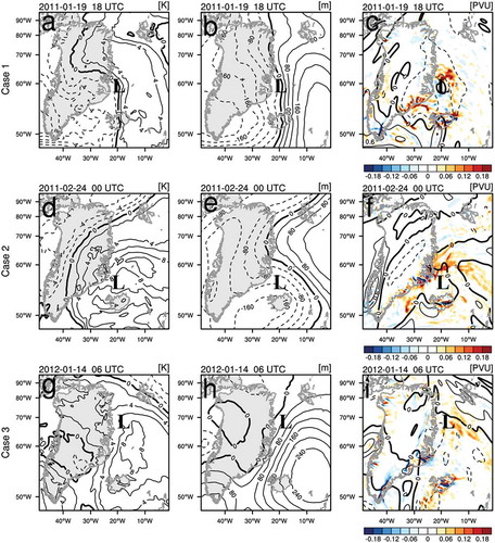
The anomaly patterns of geopotential height, temperature, and potential vorticity were also calculated at 500 hPa. The average atmospheric states for 3 months, including the case in the middle month, were used in calculating anomalies.

Results

Case study

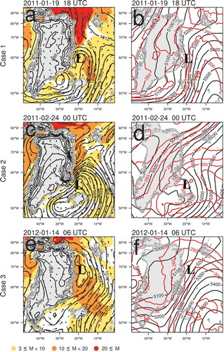
The severe gust wind speed above 20 m s⁻¹ observed in Ny-Ålesund station over Svalbard for January and February 2011–2012 is associated with the polar low developed near Svalbard. Three cases (Case 1: 20 January 2011, Case 2: 24–26 February 2011, Case 3: 14–15 January 2012) where polar lows were generated on the east coast of Greenland and induced wind speeds above 20 m s⁻¹ over Svalbard as the lows moved northward were selected. Polar lows developed rapidly within 24 hours for all three cases approaching Svalbard. To diagnose the atmospheric state when the polar lows occurred, the ERA-Interim reanalyses in the regions where the polar lows were generated (Dm in Figure 1a) were analyzed. Conditions favorable for rapidly developing polar lows were analyzed by examining the vertical instabilities of the lower atmosphere, upper air flows, and anomaly patterns. An MCAO index above 3 K appeared on the east coast of Greenland and the Greenland–Iceland–Norwegian Seas for all cases at the polar low genesis, which implies that the lower atmosphere was unstable, as shown in Businger (1985) (Figures 2a, 2c, 2e).

Figure 2. (a), (c), (e): Sea level pressure (hPa, black solid) and wind speed (m s⁻¹) at 950 hPa (black arrow) for the analysis field of ASRv2 with the marine cold air outbreaks index (M, color shading) over Greenland. (b), (d), (f): The 500 hPa geopotential height (m, black solid) and potential temperature (K, red solid) for the analysis field of ASRv2 over Greenland. The “L” represents the center of polar lows. Note that the domain is the case study domain (Dm) shown in Figure 1.

Case 1

The 1-hour average wind speed around 07 UTC on 20 January 2011 at Ny-Ålesund station was observed as 13.1 m s⁻¹, with a high wind gust of above 20 m s⁻¹ that lasted for 6 hours from 12 to 18 UTC on 20 January. The maximum wind gust was 25.1 m s⁻¹ at 14 UTC on 20 January. After the SLP was reduced rapidly by 25 hPa for 15 hours from 02 UTC on 20 January, the lowest SLP was 985.7 hPa at 17 UTC on 20 January. These radical changes in wind and pressure were the result of a polar low that developed rapidly within a few hours while quickly approaching Svalbard.

The polar low near the north of Iceland was generated at 18 UTC on 19 January 2011, 20 hours before the maximum wind gust speed was observed at Ny-Ålesund station, which was after the synoptic low moved toward the northeast approaching Iceland and separated to the north and west sides of Iceland (Figure 2a). The circulation of the low-pressure system at the lower atmosphere caused the cold air on Greenland to move to the relatively warmer Norwegian Sea, which increased the instability of the lower atmosphere on the east coast of Greenland (Figure 2a) and contributed to the explosive growth of the polar low. The low-pressure system located north of Iceland was maintained by the trough and warm advection at 500 hPa (Figure 2b). Upper atmospheric anomaly patterns and lower atmospheric vertical motion related to the generation of the polar low at 18 UTC on 19 January 2011 are shown in Figure 3. Negative anomalies of both geopotential height and temperature at 500 hPa are generally associated with positive anomalies of potential vorticity (Claud, Duchiron, and Terray 2007). In addition, the upward vertical motion at 700 hPa generally occurs in front or right of the developing cyclone (Shapiro, Fedor, and Hampel 1987; Neiman and Shapiro 1993; Ninomiya et al. 2004). Negative anomalies of both temperature and geopotential height at 500 hPa exist around the polar low genesis region (Figures 3a, 3b), and positive anomalies of potential vorticity at 500 hPa appear above and upward vertical motion at 700 hPa appears in advance of the polar low genesis region (Figure 3c), which implies that these upper and lower atmospheric conditions cause the polar low to develop rapidly. As a result, strong winds above 20 m s⁻¹ were observed at Ny-Ålesund 18 hours after the generation of the polar low.

Figure 3. (a), (d), (g): The 500 hPa anomaly of the temperature (K); (b), (e), (h): geopotential height (m); and (c), (f), (i): potential vorticity (K m² kg⁻¹ s⁻¹) for each case (positive anomaly: solid, negative anomaly: dashed) with the 700 hPa vertical wind speed (color shading) for the analysis field of ASRv2. The “L” denotes the center of polar lows. Note that the domain is the case study domain (Dm) shown in Figure 1.

Case 2

In Case 2, the 1-hour average wind speed observed at Ny-Ålesund station increased rapidly from 3.4 m s⁻¹ at 14 UTC to 14.3 m s⁻¹ at 18 UTC on 24 February 2011. A high wind gust speed above 20 m s⁻¹ lasted for 25 hours from 19 UTC on 24 February. During 13 hours of this period, a wind gust speed above 25 m s⁻¹ was observed. After the SLP rapidly reduced by 42 hPa during over 35 hours, the lowest SLP was observed to be 985.7 hPa at 20 UTC on 25 February 2011. The polar low generated to the east of Greenland developed stronger than in Case 1 and approached Svalbard more slowly, causing continuous severe wind at Ny-Ålesund.

At the beginning of the polar low genesis at 00 UTC on 24 February 2011, similar to Case 1, the synoptic low moved northward toward Iceland. The low pressure near the north of Iceland was maintained by the trough and warm advection at 500 hPa (Figures 2c, 2d). The circulation of the low in the lower atmosphere was similar to that in Case 1, moving the cold air over Greenland to the Norwegian Sea, increasing the instability in the lower atmosphere (Figure 2c). The negative anomalies of the temperature at 500 hPa approached the polar low genesis region from the west (Figure 3d), and negative anomalies of the geopotential height at 500 hPa and positive anomalies of the potential vorticity at 500 hPa were over the polar low genesis region (Figures 3e, 3f) with the upward vertical motion at 700 hPa in advance of the polar low genesis region (Figure 3f). Due to these upper and lower atmospheric conditions associated with the polar low development, strong winds above 20 m s⁻¹ were observed at Ny-Ålesund 19 hours after the generation of the polar low.

Case 3

The 1-hour average wind speed observed at Ny-Ålesund station increased rapidly from 4 m s⁻¹ at 7 UTC to 18.5 m s⁻¹ at 16 UTC on 14 January 2012. A high wind gust speed above 20 m s⁻¹ lasted for 5 hours from 14 UTC on 14 January. After the SLP rapidly reduced by 22 hPa for 20 hours, the lowest SLP was observed to be 984.8 hPa at 00 UTC on 15 January 2012. The rate of increase in the observed wind gust speed over time was moderate compared to Case 1 and Case 2 because the polar low developed more slowly in Case 3 than in Case 1 and Case 2.

At the beginning of the polar low at 06 UTC on 14 January 2012, the cyclonic circulation over the east coast of Greenland moved the cold air in the lower atmosphere on Greenland to the Norwegian Sea (Figure 2e), and the upper atmospheric divergence enhanced the development of the polar low (Figure 2f). The temperature and geopotential height anomalies at 500 hPa (Figures 3g, 3h) and potential vorticity anomalies (Figure 3i) are somewhat associated with the polar low development as in Case 1 and Case 2, although the negative anomaly patterns at 500 hPa for both temperature and geopotential height were weaker and smaller in size than those in Case 1 and Case 2. The upward vertical motion at 700 hPa appears to the right of the polar low region (Figure 3i), which is favorable for the polar low development. As a result, strong winds above 20 m s⁻¹ were observed at Ny-Ålesund 8 hours after the generation of the polar low.

Evaluation of wind forecasts

The case studies in the previous section showed that the polar lows causing severe wind in Svalbard developed strongly and rapidly. The performance of wind forecasts for each case was evaluated using the PWRF and 3DVAR DA system.

Case 1

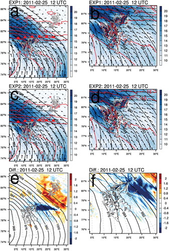
Figure 4a presents the 24-hour forecast field of Exp1 at 12 UTC on 20 January 2011 when the strong winds occurred over Svalbard. The center of the polar low was located on the west side of Svalbard (i.e., near the left boundary of the domain), and the wind speed at the center of the low was weaker than the surrounding area because the polar low developed strongly enough. Weak wind speed at the center of a polar low was also indicated in Blechschmidt, Bakan, and Graßl (2009) and Sergeev et al. (2017). The 0°C isotherm line at approximately 950 hPa shows that the warmer air in the south of Svalbard moved northward toward Svalbard. The surface warm front is located in the region where the 10-m wind direction changed abruptly. Strong wind fields formed at the rear of the warm front and were located at the front and right sides of the polar low moving northward.

Figure 4. The sea level pressure (hPa, black solid), 950 hPa temperature (K, red solid), and 10 m wind speed (m s⁻¹, color shading) and direction (black arrow) for 24-h forecast of Case1: (a) Exp1 for Dm2, (b) Exp1 for Dm3, (c) Exp2 for Dm2, and (d) Exp2 for Dm3. The sea level pressure (hPa, black solid) for 24-h forecast of Exp1 and the difference between Exp1 and Exp2 (Exp2–Exp1) for the 24-h forecast of 10 m wind speed (m s⁻¹, color shading) of Case1 for: (e) Dm2 and (f) Dm3. Note that the domain of (a), (c), and (e) is Dm2 and that of (b), (d), and (f) is Dm3, shown in Figure 1.

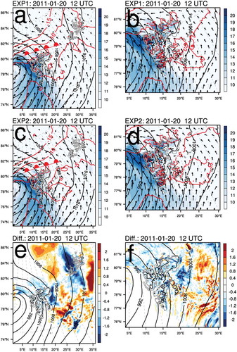
As the cold air in advance of the warm front passed over Svalbard, the wind speed on the downwind side (north slope) of the mountain was greater than that on the upwind side (south slope) of the mountain, as shown in Skeie and Grønås (2000) (Figures 4b, 4d). These wind features were simulated because the PWRF can reflect the effects of terrain on wind forecasts as the model resolution increases. Bromwich et al. (2018) showed that the ERA-Interim reanalysis with low resolution has the limitation of not being able to simulate the wind that reflects the effects of terrain in detail.

Figure 4c presents the 24-hour forecast field in Exp2 at 12 UTC on 20 January 2011. Both SLP and temperature distributions at 950 hPa in Exp1 and Exp2 are almost identical over the strong wind regions where the 10-m wind speed was over 10 m s⁻¹ but are different outside these regions (Figures 4e, 4f). The differences of wind speed between Exp1 and Exp2 appear consistently over the weak wind speed region before the strong wind fields passed over Svalbard. This means that, for the strong wind region affected by the polar low, the wind forecast accuracy in Exp2 with DA was similar to that in Exp1 without DA.

Figure 5 compares the observations and the 25-hour to 30-hour forecasts of Exp1 and Exp2 for the 10-m wind in 1-hour intervals. Because the differences in wind speed between Exp1 and Exp2 consistently appear in the weak wind regions around the polar low, the differences are greater at the beginning than at the end of the case. The wind forecasts for Exp1 and Exp2 are more similar to mean wind speed observations (AW and HAW) than gust observations (MG) at all stations, and the forecast errors of the wind speed based on HAW are smaller than those based on AW (Table 2). The average root mean square error (RMSE) for 25-hour to 30-hour forecasts of 10-m wind speed based on HAW data for all stations in Exp1 is 3.35 m s⁻¹, similar to the 24-hour wind forecast error based on 10-m AWS observations in Hines and Bromwich (2008). The wind forecast errors based on HAW data for each observation station are 1.64 m s⁻¹ and 2.09 m s⁻¹ at Sørkappøya and Hornsund (station numbers 1 and 2 in Table 1), respectively, which are smaller than those for other observation stations such as 3.49 m s⁻¹, 4.29 m s⁻¹, 4.44 m s⁻¹, and 4.16 m s⁻¹ at Sveagruva, Akseløya, Svalbard lufthavn (i.e., Svalbard Airport), and Ny-Ålesund (station numbers 3–6 in Table 1), respectively. The tendencies of the PWRF wind forecasts similar to observations in Sørkappøya and Hornsund stations are also shown in the time series of winds (Figure 5). The reduced wind forecast error in Sørkappøya and Hornsund is because the terrain has little effect on wind speed at those stations located in the southwest coast of Svalbard during the polar low passed by the west of Svalbard. Thus, if the PWRF accurately simulates the path and intensity of the polar low, then 10-m wind forecasts would be similar to the HAW in regions with low terrain effects (i.e., upwind regions). In contrast, in the stations of Sveagruva (located in the valley) and Akseløya, Svalbard lufthavn, and Ny-Ålesund, located on the downwind side (north slope of the mountain) where the terrain affects the wind forecasts, simulating wind speed accurately is difficult and the wind forecast error tended to be greater than that of the other two stations. When the wind forecasts of Exp1 in Case 1 overestimate the HAW (06–18 UTC on 20 January 2011 in Figures 5c and 5d; 16–23 UTC on 20 January 2011 in Figures 5e and 5f), the wind forecasts are relatively similar to MG. Thus, for the stations where the PWRF simulates wind speed that is much higher than AW or HAW, the wind speed forecasts are similar to MG, which implies that the performance of the PWRF in the wind speed forecasts is acceptable.

Table 2. Average forecast error statistics in Dm3, for 10-m wind speed (average value for the last 10 minutes before the observation time and highest 10-minute average wind for the last 1 hour) of each case at each observation station.

			Case1		Case2		Case3
Wind type	Site no.	Verification	Exp1 (25–30 h)	Exp2 (25–30 h)	Exp1 (25–30 h)	Exp2 (25–30 h)	Exp1 (25–30 h)	Exp2 (25–30 h)
AW	1	RMSE	1.67	1.94	3.01	3.02	3.61	3.50
		Bias	1.09	1.24	−0.03	−0.13	−0.26	−0.47
		Correlation	0.95	0.93	0.60	0.60	0.37	0.44
	2	RMSE	2.92	2.59	3.02	2.91	3.59	3.61
		Bias	1.67	1.32	1.99	1.89	0.66	0.86
		Correlation	0.68	0.75	0.87	0.88	0.39	0.41
	3	RMSE	4.75	4.67	3.40	3.35	4.40	4.12
		Bias	2.27	2.44	0.71	1.02	0.74	0.62
		Correlation	0.39	0.33	0.43	0.47	0.40	0.48
	4	RMSE	5.55	5.66	5.82	5.62	3.95	3.91
		Bias	4.07	4.68	4.30	4.27	1.09	1.02
		Correlation	0.70	0.65	0.76	0.75	0.31	0.30
	5	RMSE	5.82	5.81	5.67	5.69	5.29	5.23
		Bias	4.44	4.22	4.56	4.64	0.82	0.65
		Correlation	0.71	0.67	0.84	0.84	0.28	0.27
	6	RMSE	5.29	5.49	6.01	5.90	5.20	5.20
		Bias	3.12	3.26	4.54	4.26	1.87	1.99
		Correlation	0.72	0.69	0.85	0.83	0.51	0.50
	Average RMSE over sites		4.33	4.36	4.49	4.42	4.34	4.26
	Average bias over sites		2.78	2.86	2.68	2.66	0.82	0.78
	Average correlation over sites		0.69	0.67	0.73	0.73	0.38	0.40
HAW	1	RMSE	1.64	1.91	3.31	3.39	3.91	3.90
		Bias	0.40	0.54	−1.17	−1.27	−1.52	−1.74
		Correlation	0.90	0.87	0.61	0.59	0.37	0.43
	2	RMSE	2.09	1.86	2.02	1.94	3.80	3.73
		Bias	0.58	0.22	0.43	0.33	−0.95	−0.75
		Correlation	0.78	0.84	0.89	0.90	0.38	0.40
	3	RMSE	3.49	3.37	3.31	3.20	4.35	4.08
		Bias	1.01	1.17	−0.29	0.01	−0.43	−0.55
		Correlation	0.64	0.60	0.42	0.45	0.45	0.53
	4	RMSE	4.29	4.43	4.92	4.70	3.83	3.86
		Bias	2.71	3.33	2.97	2.95	−0.20	−0.27
		Correlation	0.78	0.72	0.76	0.75	0.32	0.29
	5	RMSE	4.44	4.42	4.38	4.38	5.43	5.43
		Bias	3.05	2.84	2.93	3.02	−0.74	−0.92
		Correlation	0.80	0.78	0.86	0.86	0.30	0.30
	6	RMSE	4.16	4.44	4.43	4.37	4.29	4.29
		Bias	1.83	1.97	2.82	2.55	0.69	0.80
		Correlation	0.80	0.77	0.85	0.84	0.62	0.62
	Average RMSE over sites		3.35	3.41	3.73	3.66	4.27	4.22
	Average bias over sites		1.60	1.68	1.28	1.27	−0.53	−0.57
	Average correlation over sites		0.78	0.76	0.73	0.73	0.41	0.43

RMSE = root mean square error; AW = average value for the last 10 minutes before the observation time; HAW = highest 10-minute average wind for the last 1 hour.

Figure 5. Time series of observations and 25-hour to 30-hour forecasts of Exp1 and Exp2 in Dm3 for 10-m wind speed (m s⁻¹) in Case 1 (AW: black solid, HAW: black dashed, MG: gray solid, Exp1: blue solid, Exp2: red solid). AW = average value for the last 10 minutes before the observation time; HAW = highest 10-minute average wind for the last 1 hour; MG = maximum gust (3 seconds) for the last 10 minutes; WMO = World Meteorological Organization.

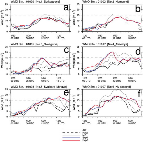
The RMSE of wind speed forecasts based on HAW in Exp2 is smaller than that of Exp1 at three (station number 2, 3, and 5 in Table 1) of six observation stations (Table 2). Thus, the wind speed forecast error of Exp2 is similar to or smaller than that of Exp1. In particular, when the wind speed forecasts in Exp1 overestimate the HAW (i.e., 9–12 UTC on 20 January 2011 in Figure 5c and 10–15 UTC on 20 January 2011 in Figure 5e), the RMSE of wind speed forecasts in Exp2 was smaller than that in Exp1 because the overestimation of wind speeds in Exp1 was reduced in Exp2 (Figures 5c, 5e).

Case 2

Figure 6a presents the 24-hour forecast field at 12 UTC on 25 February 2011. The center of the polar low was located on the west side of Svalbard (left boundary of the domain) with weaker wind speed at the center than the surrounding area. The relatively warm air moves toward Svalbard from the south. The surface warm front was located in the region where the 10-m wind direction changes abruptly. The strong wind fields formed at the front and rear of the warm front and at the front and right sides of the polar low moving northward. Unlike Case 1, in Case 2 the isotherm at 950 hPa was densely located in advance of the warm front with very strong temperature gradients that widely cause severe winds on the surface.

Figure 6. The sea level pressure (hPa, black solid), 950 hPa temperature (K, red solid), and 10 m wind speed (m s⁻¹, color shading) and direction (black arrow) for 24-h forecast of Case2: (a) Exp1 for Dm2, (b) Exp1 for Dm3, (c) Exp2 for Dm2, and (d) Exp2 for Dm3. The sea level pressure (hPa, black solid) for 24-h forecast of Exp1 and the difference between Exp1 and Exp2 (Exp2–Exp1) for the 24-h forecast of 10 m wind speed (m s⁻¹, color shading) of Case2 for: (e) Dm2 and (f) Dm3. Note that the domain of (a), (c), and (e) is Dm2 and that of (b), (d), and (f) is Dm3, shown in Figure 1.

As the model resolution increases, the effects of terrain were reflected in wind forecasts. Thus, the wind speed on the downwind side (northwest slope of mountain) is higher than that on the upwind side (southeast slope of mountain) as in Case 1 (Figures 6b, 6d).

Figure 6c represents the 24-hour forecast field with DA (Exp2) at the same time as Exp1 in Figure 6a. The distributions of both SLP and temperature at 950 hPa in Exp1 and Exp2 were almost identical over the strong wind region where the 10-m wind speed was above 10 m s⁻¹ but are different outside the strong wind region (Figures 6e, 6f). This means that the accuracy of wind forecasts in Exp1 and Exp2 was similar for the strong wind regions affected by the polar low.

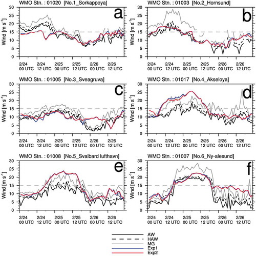
For the 10-m wind speed in Case 2, the observations are compared with the 25-hour to 30-hour forecasts of Exp1 and Exp2 at 1-hour intervals (Figure 7). The wind forecasts for Exp1 and Exp2 are more similar to AW and HAW than MG at all stations, and the wind speed forecast errors based on HAW are smaller than those based on AW (Table 2). The average RMSE for 25-hour to 30-hour forecasts of 10-m wind based on HAW data for all stations in Exp1 was 3.73 m s⁻¹, similar to that in Case 1. The wind forecast errors based on HAW data are 3.31 m s⁻¹ and 2.02 m s⁻¹ at Sørkappøya and Hornsund (station numbers 1 and 2 in Table 1), respectively, which are smaller than the forecast error for other stations such as 3.31 m s⁻¹, 4.92 m s⁻¹, 4.38 m s⁻¹, and 4.43 m s⁻¹ at Sveagruva, Akseløya, Svalbard lufthavn, and Ny-Ålesund (station numbers 3–6 in Table 1), respectively. The time series also shows the tendency of the wind forecasts to be similar to the observations at the Sørkappøya and Hornsund stations (Figure 7). In these two stations, located on the southwest coast of Svalbard, the terrain has little effect on the wind speed forecasts as the polar low passes by the west of Svalbard (as in Case 1). Therefore, if the PWRF accurately simulates the path and intensity of the polar low, then 10-m wind forecasts would be similar to the HAW in the regions less affected by terrain. When the wind forecasts of Exp1 in Case 2 overestimate the HAW (i.e., 12 UTC on 24 February to 12 UTC on 25 February 2011 in Figures 7d and 7e; 00–23 UTC on 26 February 2011 in Figure 7f), the wind forecasts follow the trend of MG. Thus, when the PWRF simulates wind speed much higher than AW or HAW, the PWRF simulates the wind speed similar to MG. Based on HAW, the RMSE of Exp2 is similar to or smaller than that of Exp1 at five of the six stations (station numbers 2–5 in Table 1; see Table 2). Consequently, in Case 2, the wind speed forecast errors of Exp2 are similar to or smaller than those of Exp1, similar to the results in Case 1.

Figure 7. Time series of observations and 25-30 h forecasts of Exp1 and Exp2 in Dm3 for 10 m wind speed (m s⁻¹) in Case 2 (AW: black solid, HAW: black dashed, MG: grey solid, Exp1: blue solid, Exp2: red solid). WMO = World Meteorological Organization.

Case 3

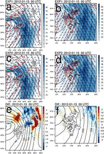
Figure 8a presents the 24-hour forecast field of Exp1 at 00 UTC on 15 January 2012 when the strong winds occurred on Svalbard. The warm front and strong wind fields were in a location similar to those in Case 1 (Figure 8a), and wind simulation reflects the terrain effects in Svalbard as the resolution increases (Figures 8b, 8d). The 24-hour forecast field of Exp2 at the same time in Exp1 is shown in Figure 8c. The wind forecast accuracy in Exp1 is similar to that in Exp2 over the strong wind region where the 10-m wind speed was above 10 m s⁻¹ (Figures 8e, 8f).

Figure 8. The sea level pressure (hPa, black solid), 950 hPa temperature (K, red solid), and 10 m wind speed (m s⁻¹, color shading) and direction (black arrow) for 24-h forecast of Case 3: (a) Exp1 for Dm2, (b) Exp1 for Dm3, (c) Exp2 for Dm2, and (d) Exp2 for Dm3. The sea level pressure (hPa, black solid) for 24-h forecast of Exp1 and the difference between Exp1 and Exp2 (Exp2–Exp1) for the 24-h forecast of 10 m wind speed (m s⁻¹, color shading) of Case 3 for: (e) Dm2 and (f) Dm3. Note that the domain of (a), (c), and (e) is Dm2 and that of (b), (d), and (f) is Dm3, shown in Figure 1.

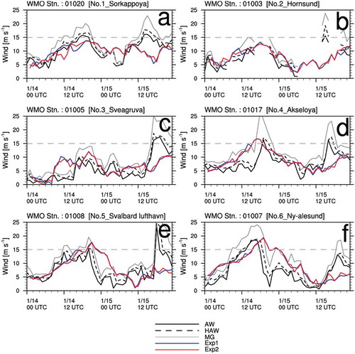
The observations and the 25-hour to 30-hour forecasts of Exp1 and Exp2 for the 10-m wind speed at 1-hour intervals are shown in Figure 9. As in Case 1 and Case 2, the wind forecasts for Exp1 and Exp2 are more similar to AW and HAW than MG at all stations, and the forecast errors of the wind speed based on HAW were smaller than those based on AW (Table 2). The average RMSE of 25-hour to 30-hour forecasts for 10-m wind, based on HAW data for all stations in Exp1, is 4.27 m s⁻¹, greater than those in Case 1 and Case 2. This is because the PWRF could not precisely simulate rapidly increasing wind speed at the end of the case. In Case 3, the polar low was redeveloped just before its extinction (17 UTC on 15 January 2012 in Figure 9). The wind forecast errors based on HAW data were 3.91 m s⁻¹ and 3.80 m s⁻¹ at Sørkappøya and Hornsund (station numbers 1 and 2 in Table 1), respectively, which are smaller than those for other stations such as 4.35 m s⁻¹, 3.83 m s⁻¹, 5.43 m s⁻¹, and 4.29 m s⁻¹ at Sveagruva, Akseløya, Svalbard lufthavn, and Ny-Ålesund (station numbers 3–6 in Table 1), respectively. As in Case 1 and Case 2, the relatively similar forecasts to the observations at the Sørkappøya and Hornsund stations (Figure 9) are due to little terrain effects on wind speed forecasts at the two stations. When the wind forecasts of Exp1 overestimate the HAW (11–16 UTC on 14 January 2012 in Figure 9d; 20 UTC 14 to 04 UTC on 15 January 2012 in Figure 9f), the wind forecasts followed the trend of MG. Based on HAW, the RMSE of Exp2 is similar to or smaller than that of Exp1 at five of the six stations (station numbers 1, 2, 3, 5, and 6 in Table 1; see Table 2). Thus, in Case 3, the wind speed forecast errors of Exp2 were similar to or smaller than the errors of Exp1, as in Case 1 and Case 2.

Figure 9. Time series of observations and 25-30 h forecasts of Exp1 and Exp2 in Dm3 for 10 m wind speed (m s⁻¹) in Case 3 (AW: black solid, HAW: black dashed, MG: grey solid, Exp1: blue solid, Exp2: red solid). WMO = World Meteorological Organization.

Evaluation of SLP forecasts

Case 1

The average RMSE of the SLP forecasts for all stations in Exp1 was 2.08 hPa (Table 3). At 17 UTC on 20 January 2011, when the lowest SLP was observed in Ny-Ålesund, the SLP forecasts in Exp1 show a positive deviation of 4.4 hPa average for all stations. Kumar, Roy Bhowmik, and Das (2012) also show that the PWRF overestimates the SLP approximately 3–4 hPa. Compared to Exp1, both the average RMSE and bias of SLP forecasts in Exp2 decrease at all observation stations (Table 3). The SLP forecasts in Exp2 are more accurate than those in Exp1, which affects the improvement of the 10-m wind speed forecasts.

Table 3. Average forecast error statistics in Dm3 for the sea level pressure of each case at each observation station.

		Case1		Case2		Case3
Site No.	Verification	Exp1 (25–30 h)	Exp2 (25–30 h)	Exp1 (25–30 h)	Exp2 (25–30 h)	Exp1 (25–30 h)	Exp2 (25–30 h)
1	RMSE	2.16	2.13	3.03	3.02	2.08	2.07
	Bias	1.79	1.76	−2.88	−2.87	1.28	1.24
	Correlation	0.98	0.98	1.00	1.00	0.99	0.99
2	RMSE	1.85	1.77	3.11	3.10	1.21	1.21
	Bias	1.48	1.40	−2.93	−2.93	0.18	0.17
	Correlation	0.98	0.98	1.00	1.00	0.00	0.00
3	RMSE	2.25	2.22	3.40	3.40	2.43	2.43
	Bias	1.14	1.08	−3.29	−3.31	1.04	1.03
	Correlation	0.98	0.98	1.00	1.00	0.99	0.99
4	RMSE	2.30	2.24	3.81	3.74	2.82	2.82
	Bias	1.45	1.35	−3.62	−3.56	1.40	1.40
	Correlation	0.98	0.98	1.00	1.00	0.99	0.99
5	RMSE	1.82	1.81	3.66	3.64	3.19	3.17
	Bias	0.97	0.95	−3.54	−3.52	1.44	1.44
	Correlation	0.98	0.98	1.00	1.00	0.98	0.98
6	RMSE	2.13	2.12	3.43	3.39	2.94	2.94
	Bias	0.83	0.73	−3.27	−3.24	1.40	1.43
	Correlation	0.98	0.98	1.00	1.00	0.98	0.98
Average RMSE over sites		2.09	2.05	3.41	3.38	2.45	2.44
Average bias over sites		1.28	1.21	−3.26	−3.24	1.12	1.12
Average correlation over sites		0.98	0.98	1.00	1.00	0.82	0.82

RMSE = root mean square error.

Case 2

In Case 2, the average RMSE of the SLP for all stations in Exp1 was approximately 3.41 hPa (Table 3). Different from Case 1, the SLP forecasts in Exp1 in Case 2 show negative deviations of 3.26 hPa on average across all observation stations. This tendency was similar around 10 UTC on 26 February 2011, when the minimum SLP appeared in Ny-Ålesund. Compared to Exp1, the RMSE of SLP forecasts in Exp2 was reduced at five of the six stations (station numbers 1, 2, 4, 5, and 6 in Table 1), and the bias of SLP forecasts in Exp2 was reduced at four of the six stations (station numbers 1, 4, 5, and 6 in Table 1; see Table 3). In particular, at the beginning of Case 2, the negative bias of SLP forecasts shown in Exp1 was reduced in Exp2.

Case 3

In Case 3, the average RMSE of the SLP for all stations in Exp1 is 2.4 hPa (Table 3). The minimum SLP was observed at 17 UTC on 15 January 2012 in Ny-Ålesund. The SLP forecasts showed a positive deviation of 7.18 hPa on average around 17 UTC on 15 January 2012 when the minimum SLP was observed. This large deviation influenced the large wind forecast error of 10 m s⁻¹ at that time (Figure 9). Compared to Exp1, the RMSE of the SLP forecasts in Exp2 was reduced at two of the six observation stations (station numbers 1 and 5 in Table 1), and the bias of SLP forecasts in Exp2 was reduced at three of the six observation stations (station numbers 1, 2, and 3 in Table 1; see Table 3). Compared to Case 1 and Case 2, the improvement in the wind forecast accuracies is neutral when using the DA in Exp2 compared to Exp1.

Summary and discussion

In this study, the performance of the high-resolution PWRF using the ERA-Interim reanalysis as the initial conditions (Exp1) was evaluated for severe wind cases over Svalbard, where many research institutes are located. In addition, the performance of the analysis–forecast cycling system using the PWRF and 3DVAR DA system (Exp2) was also evaluated and compared with that of the cold start system (Exp1) for the same cases.

The wind speed forecasts of both Exp1 and Exp2 were most similar to the highest 10-minute average wind speed for the last 1 hour (HAW), and the average RMSE of wind speed forecast in Exp1 based on HAW was 3.78 m s⁻¹ for six stations for three of the cases. When the wind forecasts of Exp1 and Exp2 overestimated HAW, the wind speed forecasts followed the trend of MG. The differences between wind speed forecasts in Exp1 and Exp2 were large at the beginning of the case before the front passed over Svalbard because the differences are present not in the strong wind region where the 10-m wind speed was above 10 m s⁻¹ but in the weak wind region around the front. The RMSE in Exp2 with DA was generally smaller than that in Exp1 without DA. When the forecasts in Exp1 overestimated the average wind speed observation, the overestimation was reduced in Exp2. For the SLP forecast, both forecasts in Exp1 and Exp2 were generally similar to the observations. However, neither experiment could simulate the rapidly decreasing SLP, which caused an increase in the wind speed forecast error. When the positive (negative) bias of the SLP forecasts in Exp1 appeared against observations, the SLP forecasts in Exp2 simulated SLP lower (higher) than those in Exp1, which reduced the bias.

Since the wind speed forecasts at 10 m in the range of the average wind and gust, the accuracy of the wind speed forecasts in the PWRF was generally high. The forecasts in Exp2 were produced in the small domain (Dm2), which is limited to simulate polar lows. Furthermore, the number of observations in Dm2 was limited. Despite these constraints, the forecast performance of Exp2 with DA is comparable to or even better than that in Exp1 using reanalysis as the initial condition. This implies that the analysis–forecast cycling system with DA is more useful than the cold start system in forecasting the polar environment. However, differences between the wind speed forecasts of Exp1 and Exp2 are primarily found in the region of weak wind, indicating that there is room for improvement by using more appropriate DA methods that consider the limited surface and upper observations. Assimilating more observations, designing an optimal observation network, and applying more appropriate DA methods would be future steps that can improve weather forecasting in the polar region.

Acknowledgments

The authors appreciate the reviewers’ valuable comments. The authors also appreciate Dr. Keith Hines from Ohio State University for providing the Polar WRF model and the Norwegian Meteorological Institute for providing observation data through the eKlima site.

Disclosure statement

No potential conflict of interest was reported by the authors.

Additional information

Funding

This work was supported by the Korea Polar Research Institute (KOPRI, PN19081) and a National Research Foundation of Korea (NRF) grant funded by the South Korean government (Ministry of Science and ICT, Grant 2017R1E1A1A03070968). The simulations were mostly carried out by utilizing the supercomputer system supported by the National Center for Meteorological Supercomputer of Korea Meteorological Administration (KMA).

References

- Ágústsson, H., H. Ólafsson, M. O. Jonassen, and Ó. Rögnvaldsson. 2014. The impact of assimilating data from a remotely piloted aircraft on simulations of weak-wind orographic flow. Tellus A 66:25421. doi:10.3402/tellusa.v66.25421.
- Aspelien, T., T. Iversen, J. B. Bremnes, and I.-L. Frogner. 2011. Short-range probabilistic forecasts from the Norwegian limited-area EPS: Long-term validation and a polar low study. Tellus A 63:564–84. doi:10.1111/j.1600-0870.2010.00502.x.
- Blechschmidt, A.-M., S. Bakan, and H. Graßl. 2009. Large-scale atmospheric circulation patterns during polar low events over the Nordic seas. Journal of Geophysical Research 114:D06115. doi:10.1029/2008JD010865.
- Bromwich, D. H., K. M. Hines, and L.-S. Bai. 2009. Development and testing of Polar Weather Research and Forecasting model: 2. Arctic Ocean. Journal of Geophysical Research 114:D08122. doi:10.1029/2008JD010300.
- Bromwich, D. H., A. B. Wilson, L. Bai, Z. Liu, M. Barlage, C.-F. Shih, S. Maldonado, K. M. Hines, S.-H. Wang, J. Woollen, et al. 2018. The Arctic system reanalysis, version 2. Bulletin of the American Meteorological Society 99:805–28. doi:10.1175/BAMS-D-16-0215.1.
- Businger, S. 1985. The synoptic climatology of polar low outbreaks. Tellus A 37:419–32. doi:10.3402/tellusa.v37i5.11686.
- Chen, F., K. E. Mitchell, J. Schaake, Y. Xue, H.-L. Pan, V. Koren, Q. Y. Duan, M. Ek, and A. Betts. 1996. Modeling of land surface evaporation by four schemes and comparison with FIFE observations. Journal of Geophysical Research 101:7251–68. doi:10.1029/95JD02165.
- Claremar, B., F. Obleitner, C. Reijmer, V. Pohjola, A. Waxegard, F. Karner, and A. Rutgersson. 2012. Applying a mesoscale atmospheric model to Svalbard glaciers. Advances in Meteorology 2012:321649. doi:10.1155/2012/321649
- Claud, C., B. Duchiron, and P. Terray. 2007. Associations between large-scale atmospheric circulation and polar low developments over the North Atlantic during winter. Journal of Geophysical Research 112:D12101. doi:10.1029/2006JD008251.
- Dee, D. P., S. M. Uppala, A. J. Simmons, P. Berrisford, P. Poli, S. Kobayashi, U. Andrae, M. A. Balmaseda, G. Balsamo, P. Bauer, et al. 2011. The ERA-Interim reanlaysis: Configuration and performance of the data assimilation system. Quarterly Journal of the Royal Meteorological Society 137:553–97. doi:10.1002/qj.v137.656.
- Grell, G. A., and D. Devenyi. 2002. A generalized approach to parameterizing convection combining ensemble and data assimilation techniques. Geophysical Research Letters 29(14):38-1-38-4.
- Grønås, S., and N. G. Kvamstø. 1995. Numerical simulations of the synoptic conditions and development of Arctic outbreak polar lows. Tellus A 47:797–814. doi:10.3402/tellusa.v47i5.11576.
- Hines, K. M., and D. H. Bromwich. 2008. Development and testing of Polar Weather Research and Forecasting (WRF) model. Part I: Greenland ice sheet meteorology. The Monthly Weather Review 136:1971–89. doi:10.1175/2007MWR2112.1.
- Hines, K. M., D. H. Bromwich, L. Bai, C. M. Bitz, J. G. Powers, and K. W. Manning. 2015. Sea ice enhancements to Polar WRF. The Monthly Weather Review 143:2363–85. doi:10.1175/MWR-D-14-00344.1.
- Hines, K. M., D. H. Bromwich, L.-S. Bai, M. Barlage, and A. G. Slater. 2011. Development and testing of Polar WRF. Part III: Arctic land. The Journal of Climate 24:26–48. doi:10.1175/2010JCLI3460.1.
- Hong, S.-Y., J. Dudhia, and S.-H. Chen. 2003. A revised approach to ice-microphysical processes for the bulk parameterization of cloud and precipitation. The Monthly Weather Review 132:103–20. doi:10.1175/1520-0493(2004)132<0103:ARATIM>2.0.CO;2.
- Iacono, M. J., J. S. Delamere, E. J. Mlawer, M. W. Shephard, S. A. Clough, and W. D. Collins. 2008. Radiative forcing by long-lived greenhouse gases: Calculations with the AER radiative transfer models. Journal of Geophysical Research 113:D13103. doi:10.1029/2008JD009944.
- Irvine, E. A., S. L. Gray, and J. Methven. 2011. Forecast impact of targeted observations: Sensitivity to observation error and proximity to steep orography. The Monthly Weather Review 139:69–78. doi:10.1175/2010MWR3459.1.
- Janjić, Z. I. 1994. The step-mountain eta coordinate model: Further developments of the convection, viscous sublayer and turbulence closure schemes. The Monthly Weather Review 122:927–45. doi:10.1175/1520-0493(1994)122<0927:TSMECM>2.0.CO;2.
- Jung, T., N. D. Gordon, P. Bauer, D. H. Bromwich, M. Chevallier, J. J. Day, J. Dawson, F. Doblas-Reyes, C. Fairall, H. F. Goessling, et al. 2016. Advancing polar prediction capabilities on daily to seasonal time scales. Bulletin of the American Meteorological Society 97:1631–47. doi:10.1175/BAMS-D-14-00246.1.
- Kilpeläinen, T., T. Vihma, M. Manninen, A. Sjoblom, E. Jakobson, T. Palo, and M. Maturilli. 2012. Modelling the vertical structure of the atmospheric boundary layer over Arctic fjords in Svalbard. Quarterly Journal of the Royal Meteorological Society 138:1867–83. doi:10.1002/qj.1914.
- Kilpeläinen, T., T. Vihma, and H. Olafsson. 2011. Modelling of spatial variability and topographic effects over Arctic fjords in Svalbard. Tellus A 63:223–37. doi:10.1111/j.1600-0870.2010.00481.x.
- Klein, T., and G. Heinemann. 2002. Interaction of katabatic winds and mesocyclones near the eastern coast of Greenland. Meteorological Applications 9:407–22. doi:10.1017/S1350482702004036.
- Kolstad, E. W. 2011. A global climatology of favourable conditions for polar lows. Quarterly Journal of the Royal Meteorological Society 137:1749–61. doi:10.1002/qj.888.
- Kolstad, E. W. 2017. Higher ocean wind speeds during marine cold air outbreaks. Quarterly Journal of the Royal Meteorological Society 143:2084–92. doi:10.1002/qj.2017.143.issue-706.
- Kristiansen, J., S. J. Sørland, T. Iversen, D. Bjørge, and M. Ø. Køltzow. 2011. High-resolution ensemble prediction of a polar low development. Tellus A 63:585–604. doi:10.1111/j.1600-0870.2010.00498.x.
- Kristjánsson, J. E., I. Barstad, T. Aspelien, I. Føre, Ø. Godøy, Ø. Hov, E. Irvine, T. Iversen, E. Kolstad, T. E. Nordeng, et al. 2011. The Norwegian IPY-THORPEX polar lows and Arctic fronts during the 2008 Andøya campaign. Bulletin of the American Meteorological Society 92:1443–66. doi:10.1175/2011BAMS2901.1.
- Kumar, A., S. K. Roy Bhowmik, and A. K. Das. 2012. Implementation of Polar WRF for short range prediction of weather over Maitri region in Antarctica. The Journal of Earth System Science 121:1125–43. doi:10.1007/s12040-012-0217-3.
- Mayer, S., M. O. Jonassen, A. Sandvik, and J. Reuder. 2012. Profiling the Arctic stable boundary layer in Advent Valley, Svalbard: Measurements and simulations. Boundary-Layer Meteorology 143:507–26. doi:10.1007/s10546-012-9709-6.
- Monin, A. S., and A. M. Obukhov. 1954. Basic laws of turbulent mixing in the surface layer of the atmosphere. Contributions of the Geophysical Institute, Slovak Academy of Sciences 24:163–87.
- Moore, G. W. K., I. A. Renfrew, B. E. Harden, and S. H. Mernild. 2015. The impact of resolution on the representation of southeast Greenland barrier winds and katabatic flows. Geophysical Research Letters 42(8): 3011-8 doi:10.1002/2015GL063550.
- Nakanishi, M., and H. Niino. 2006. An improved Mellor-Yamada level-3 model: Its numerical stability and application to a regional prediction of advection fog. Boundary-Layer Meteorology 119:397–407. doi:10.1007/s10546-005-9030-8.
- Neiman, P. J., and M. A. Shapiro. 1993. The life cycle of an extratropical marine cyclone. Part I: Frontal-cyclone evolution and thermodynamic air-sea interaction. The Monthly Weather Review 121:2153–76. doi:10.1175/1520-0493(1993)121<2153:TLCOAE>2.0.CO;2.
- Ninomiya, K., T. Nishimura, T. Enomoto, T. Suzuki, and S. Matsumura. 2004. Generation and development of a polar mesoscale cyclone over the east coast of Asia as simulated in an AGCM. Journal of the Meteorological Society of Japan 82 (5):1435–46. doi:10.2151/jmsj.2004.1435.
- Parrish, D. F., and J. C. Derber. 1992. The National Meteorological Center’s spectral statistical-interpolation analysis system. The Monthly Weather Review 120:1747–63. doi:10.1175/1520-0493(1992)120<1747:TNMCSS>2.0.CO;2.
- Powers, J. G., K. W. Manning, D. H. Bromwich, J. J. Cassano, and A. M. Cayette. 2012. A decade of Antarctic science support through AMPS. Bulletin of the American Meteorological Society 93:1699–712. doi:10.1175/BAMS-D-11-00186.1.
- Rasmussen, E. A., and J. Turner. 2003. Polar lows: Mesoscale weather systems in the polar regions. Cambridge, UK: Cambridge Univ. Press.
- Sauter, T., M. Möller, R. Finkelnburg, M. Grabiec, D. Scherer, and C. Schneider. 2013. Snowdrift modelling for the Vestfonna ice cap, north-eastern Svalbard. The Cryosphere 7:1287–301. doi:10.5194/tc-7-1287-2013.
- Sergeev, D. E., I. A. Renfrew, T. Spengler, and S. R. Dorling. 2017. Structure of a shear-line polar low. Quarterly Journal of the Royal Meteorological Society 143:12–26. doi:10.1002/qj.2017.143.issue-702.
- Shapiro, M. A., L. S. Fedor, and T. Hampel. 1987. Research aircraft measurements of a polar low over the Norwegian Sea. Tellus 39A:272–306. doi:10.1111/j.1600-0870.1987.tb00309.x.
- Skeie, P., and S. Grønås. 2000. Strongly stratified easterly flows across Spitsbergen. Tellus A 52:473–86. doi:10.3402/tellusa.v52i5.12281.
- Smirnova, J., and P. Golubkin. 2017. Comparing polar lows in atmospheric reanalysis: Arctic system reanalysis versus ERA-Interim. The Monthly Weather Review 145:2375–83. doi:10.1175/MWR-D-16-0333.1.
- Sukoriansky, S., B. Galperin, and V. Perov. 2005. Application of a new spectral theory of stably stratified turbulence to the atmospheric boundary layer over sea ice. Boundary-Layer Meteorology 117:231–57. doi:10.1007/s10546-004-6848-4.
- Tilinina, N., S. K. Gulev, and D. H. Bromwich. 2014. New view of Arctic cyclone activity from Arctic system reanalysis. Geophysical Research Letters 41:1766–72. doi:10.1002/2013GL058924.
- Wilson, A. B., D. H. Bromwich, and K. M. Hines. 2011. Evaluation of Polar WRF forecasts on the Arctic System Reanalysis domain: Surface and upper air analysis. Journal of Geophysical Research 116:D11112. doi:10.1029/2010JD015013.
- Zappa, G., and L. Shaffrey. 2014. Can polar lows be objectively identified and tracked in the ECMWF operational analysis and the ERA-Interim reanalysis? The Monthly Weather Review 142:2596–608. doi:10.1175/MWR-D-14-00064.1.