Soil organic carbon predictions in Subarctic Greenland by visible–near infrared spectroscopy

ABSTRACT

Release of carbon from high-latitude soils to the atmosphere may have significant effects on Earth’s climate. In this contribution, we evaluate visible–near-infrared spectroscopy (vis-NIRS) as a time- and cost-efficient tool for assessing soil organic carbon (SOC) concentrations in South Greenland. Soil samples were collected at two sites and analyzed with vis-NIRS. We used partial least square regression (PLS-R) modeling to predict SOC from vis-NIRS spectra referenced against in situ dry combustion measurements. The ability of our approach was validated in three setups: (1) calibration and validation data sets from the same location, (2) calibration and validation data sets from different locations, and (3) the same setup as in (2) with the calibration model enlarged with few samples from the opposite target area. Vis-NIRS predictions were successful in setup 1 (R² = 0.95, root mean square error of prediction [RMSEP] = 1.80 percent and R² = 0.82, RMSEP = 0.64 percent). Predictions in setup 2 had higher errors (R² = 0.90, RMSEP = 7.13 percent and R² = 0.78, RMSEP = 2.82 percent). In setup 3, the results were again improved (R² = 0.95, RMSEP = 2.03 percent and R² = 0.77, RMSEP = 2.14 percent). We conclude that vis-NIRS can obtain good results predicting SOC concentrations across two subarctic ecosystems, when the calibration models are augmented with few samples from the target site. Future efforts should be made toward determination of SOC stocks to constrain soil–atmosphere carbon exchange.

KEYWORDS:

• Soil organic carbon
• visible–near-infrared spectroscopy
• subarctic
• Greenland

Introduction

Soils are a heterogeneous material mixture consisting of various components, among which soil organic carbon plays a crucial role. The relative amount of organic carbon in the soil matrix (% SOC) affects soil fertility and a number of other soil properties, such as pH, soil structure, soil–water retention, and plant nutrient supply. Northern circumpolar soils represent substantial carbon storage (i.e., 1,672 Pg; Tarnocai et al. 2009) compared to the biosphere (560 Pg) and the atmosphere (760 Pg) on a global scale (Lal 2004). Soils can affect Earth’s future climate, interacting with the atmosphere, acting as either a source or sink for carbon emissions, such as CO₂ and CH₄ (Lal 2004). To quantify these soil–atmosphere carbon fluxes, determination of SOC stocks is essential. The calculation relies on the absolute amount of SOC in a soil volume, including SOC concentration (%), soil bulk density (g/m³), coarse fraction (CF %), and soil depth (m). In particular, SOC concentrations have a strong control on SOC stock calculations. For example Hoffmann, Hoffmann, Johnson, and Kuhn (2014) showed that in mountain environments the correlation coefficient between the two variables is 0.54, compared to the bulk density (0.07) and the coarse fraction (0.14). Therefore, this study focuses on determination of SOC concentration.

Extensive research has been done on the quantification of SOC stocks on a global scale (e.g., Post et al. 1982; Batjes 1996; Scharlemann et al. 2014). Nonetheless, SOC studies are still extremely sparse in wide areas of the Arctic, where the climate impact may be particularly high (IPCC 2014) and the carbon stock may be substantial (McGuire et al. 2009; Tarnocai et al. 2009). The most obvious reasons for this lack of research activity in arctic areas are the challenging accessibility, lack of infrastructure and transportation facilities, and short fieldwork seasons limited to the summer months, resulting in costly data acquisition. Among the arctic study areas, subarctic regions, typically defined as areas extending between 50° N and 70° N, are commonly underrepresented. This may be because the High Arctic is considered to have most pronounced effects on climate warming (Serreze and Francis 2006; McGuire et al. 2009). However, subarctic environments have highly complex pedological systems (Walker et al. 2004) and, due to their recent exposure from the glacial cover, they are constantly exposed to ongoing erosion and weathering processes. Moreover, the observed increase in air temperature in subarctic regions may contribute to future prospects for developing agriculture.

Several studies estimated SOC stocks in the Arctic on a local scale, including northeast European Russia (Kuhry et al. 2002), northwest Greenland (Burnham and Sletten 2010), the central Canadian Arctic (Hugelius et al. 2010), and northeast Greenland and northeast Siberia (Palmtag et al. 2014). These studies have recognized a significant variation in SOC concentrations and stocks between and within the different regions, which is an additional challenge for an extrapolation of SOC stocks to the entire Arctic (Banerjee et al. 2011). Campeau, Lafleur, and Humphreys (2014) demonstrated that the SOC stock in the central Canadian Arctic varies on a small scale of a couple of meters. The small-scale variation in SOC stocks has been recognized in other remote environments; for example, in alpine settings (Hoffmann, Hoffmann, Jurasinski, et al. 2014). The small-scale heterogeneity of SOC concentrations and other soil properties may result in large uncertainties when averaging over large areas (Hoffmann, Hoffmann, Johnson, and Kuhn 2014; Hoffmann, Hoffmann, Jurasinski, et al. 2014). Therefore, it is crucial to use time- and cost-effective techniques for robust SOC concentration predictions that are able to also depict small-scale variability.

The above mentioned studies have applied an elemental analyzer to determine SOC concentrations. This is a sample-destructive technique based on dry combustion at elevated temperatures (i.e., above 1300°C) with the collection and detection of evolved CO₂ (Schumacher 2002). This technique requires thorough sample preparation (drying, sieving, and sample homogenization), and maintenance of the instrument is often costly.

In the past few decades, visible–near-infrared spectroscopy (vis-NIRS) has proved to be an efficient alternative to traditional techniques (i.e., dry combustion, loss on ignition, etc.) for SOC determination (Malley, Martin, and Ben-Dor 2004; Stenberg et al. 2010; Soriano-Disla et al. 2014). Vis-NIRS is a simpler and quicker procedure for data collection and analysis compared to traditional methods. Estimates show that a vis-NIRS measurement of organic carbon is about three to ten times cheaper than conventional wet chemistry methods (O’Rourke and Holden 2011). The technique is based on measurement of the reflectance of the soil samples in the visible and near-infrared range (350–2,500 nm), which can be analyzed by applying multivariate data analysis (Viscarra Rossel et al. 2006). There are several statistical tools used to model the relationship between the spectra data and soil properties; for instance, partial least squares regression (PLS-R; Sjöström et al. 1983; Vohland et al. 2011).

Although many studies aimed to predict SOC concentrations using vis-NIRS around the world (e.g., Volkan Bilgili et al. 2010; Summers et al. 2011; Stevens et al. 2013), it has been only applied in a small number of studies in the Arctic. This is probably due to generally coarser soil texture and lower organic carbon concentrations in arctic soils, which often result in poorer vis-NIRS predictions for SOC concentrations. Rinnan and Rinnan (2007) used NIRS to measure the quality of soil organic matter in an experimental pitch in northern Sweden. They found that NIRS was a suitable technique for soil organic matter predictions in highly organic arctic soils (R² > 0.9) when compared to a reference data set based on the loss on ignition technique. Guy, Siciliano, and Lamb (2015) successfully predicted SOC concentrations of polar desert soils in the Canadian High Arctic (R² = 0.91) with an in situ vis-NIRS technique (i.e., spectral data were collected directly in the field with a portable vis-NIR spectrometer). Their regional prediction models (i.e., using a local model to predict SOC in three polar desert locations across Ellesmere Island) showed poor prediction accuracy, with R² from 0.07 to 0.36, which was improved when the local model was enlarged with regional samples (R² between 0.69 and 0.86).

The approach of enlarging local models with regional samples to obtain better NIRS predictions on a regional scale has been used in several other studies in geographically different regions (e.g., Sankey et al. 2008; Peng et al. 2015). The compilation of a spectral library including regions of contrasting geological, soil, and hydrological properties may substantially increase the prediction ability of the models for local application (Shepherd and Walsh 2002; Gogé et al. 2012). This approach could be a solution to increasing data coverage at reduced costs for sampling in remote areas.

In this study, we investigate the application of vis-NIRS as a tool for the prediction of SOC concentrations (%) in two areas in South Greenland (Upernaviarsuk and Søndre Igaliku). The specific aims of this article are to (1) assess the ability of vis-NIRS for site-specific (calibration and validation data set from the same region) predictions of SOC in Upernaviarsuk and Søndre Igaliku, (2) evaluate site-wise (calibration and validation data set from different regions) vis-NIRS predictions of SOC, and (3) test whether site-specific models augmented with representative samples from the target area yield better site-wise predictions.

Materials and methods

Study area

The study area includes a topographically diverse terrain defined by a deep and narrow, generally northeast–southwest-orientated fjord valley, Igalikup Kangerlua, extending from the inner ice sheet to the Labrador Sea. Soil samples were collected at two sites: in the vicinity of Upernaviarsuk (60°44ʹ59ʺ N 45°53ʹ23ʺ W; sampled area: approximately 5 km²; denoted as UPA in the following) and in the vicinity of Søndre Igaliku (60°53ʹ31ʺ N 45°16ʹ16ʺW; sampled area: approximately 30 km²; denoted as SIA; Figure 1). The samples were collected between sea level and 210 m elevation for the UPA and between the sea level and 646 m for the SIA.

Figure 1. Study area and sampling sites (bold) in South Greenland.

Both investigated areas are characterized by a continental subarctic climate (Cappelen 2011); however, a distinct climatic gradient is apparent between the two regions: lower summer temperatures (mean summer temperature 4°C) and higher yearly precipitation (approximately 850 mm) dominate the UPA, and warmer summer seasons (mean summer temperature 8°C) and lower yearly precipitation (approximately 600 mm) prevail in the SIA (Jakobsen 1991a; Cappelen 2011). This climatic gradient defines the abundance of vegetation and consequently soil development and soil carbon storage in the region. The vegetation type in the UPA is classified as subarctic heath defined by low bushes of subarctic birch and willow alternating with open grass communities. Due to higher summer temperatures, the vegetation is much more luxuriant in the protected valleys of SIA, where at lower elevations (up to 200 m) willow and birch shrubland can reach up to 2 m height. In the SIA, numerous fens and bogs are found around lakes and streams (Jakobsen 1991b; Fredskild 1992). Another factor impacting soil development in the region is the time of exposure from glacial coverage (Fredskild 1992). Because the SIA is located closer to the present-day margin of the Greenland Ice Sheet, it can be expected that the UPA was ice-free earlier in geological history. Sørensen and Andersen(2006) reported that the area of Narsaq (approximately 20 km north-northwest of the UPA) has been ice-free since approximately 10,200–10,400 years ago, and the area of Narsarsuaq (approximately 30 km north-northwest of the SIA) has been ice-free since 9,500–9,700 years ago. A differentiation in the soil matrix is furthermore generated by the deposition of sandy loess material, resulting from strong foehn winds eroding the bedrock and soils throughout the Holocene (Jakobsen 1991b; Fredskild 1992; Massa et al. 2012). In the SIA, the wind-eroded material is deposited in wind-protected locations outside the glacial margin and represents the major parent material for the soils at this site. The sandy to silty (loess) eolian sediments exceed a thickness of locally more than 2 m and overlay coarse moraine deposits. In contrast, the deposition of the eolian material is very limited in the UPA. Instead, coarse-textured ablation tills and marine deposits form the major parent material with a thin cover (~2 cm) of eolian sediments.

In the vicinity of the SIA, Jacobsen (1987) described a soil profile where 46 cm of young eolian sediments was deposited over older, well-developed podzol (34 cm deep), resulting in a polypedon. The eolian sediments showed only weakly developed horizons, including eluvial and illuvial horizons. The organic matter concentration of the young sediments varied between 4.2 percent (top horizon) and 2.4 percent (bottom horizon), whereas 2.2 percent (top) and 0.7 percent (bottom) were estimated for the older podzol. The soil texture of the eolian sediment was described as loamy sand. Generally, the texture of the underlying podzol was characterized as sandy loam with a small percentage of pebbles and cobbles (0.05 percent–0.84 percent). Jakobsen (1989) presented a detailed description of a 45-cm-deep soil profile in the UPA. The profile consists of five horizons (Ah, Ae, Bs1, Bs2, and C) with SOC concentrations ranging from 15.24 percent (Ah), to 2.16 percent (Ae), to 1.15 percent (C). The soil texture is described as silty loam, with the sand fraction increasing with depth (from 43 percent to 68 percent, top to bottom layer).

During the sample collection for our study, soil profiles with a well-developed bleached-E horizon, characteristic of podzols, were observed at several locations in the SIA. The soil profiles in the UPA were rarely developed more than 35 cm above the coarse-textured parent material. The upper horizons were commonly humus rich, and evidence of weakly developed podzolation was usually observed in low-lying sites with coarse-textured soils.

Sampling and laboratory analysis

Bulk soil samples were collected during two separate field expeditions: In 2013, the UPA soils were sampled from ninety-three soil pits, resulting in 173 samples. In 2015, the SIA soils were sampled from fifty-eight soil pits, resulting in 157 samples. The soils were sampled to a maximum depth of 20 cm in the UPA. Sampling depths at several locations in the SIA reached 50 cm or more and, where possible, bulk samples were obtained at every 5-cm depth until the parent material or a lithic or paralithic contact was reached. The individual bulk soil samples were collected with a 100-cm³ stainless steel soil sample ring, replicated three times at each depth. This sampling technique enables calculation of bulk densities (g/cm³) based on total soil weight and the volume of the ring. Though the sample collection was consistent for the two field campaigns, the sampling strategy was different. The samples were collected on an approximately 250 m grid sequence across the UPA, whereas ten to fifteen samples were randomly distributed across different pre-identified land cover or land use classes derived from SPOT satellite imagery for the SIA region.

The samples were transported to laboratory facilities in Denmark, where they were air dried and sieved to a 2-mm fraction. A portion of each sample was ball-milled to less than 63 µm and oven dried at 100°C for 24 hours before being analyzed for total carbon by dry combustion at 1050°C (VarioMax CNS Elementar Analyzer GmbH, Hanau, Germany). The basic principle of the dry combustion technique is the destruction of soil organic matter at high temperatures. All forms of carbon in the sample are converted to CO₂, which is subsequently quantified by a gravimetric technique (Nelson and Sommers 1996; Schumacher 2002). Because geological records of the bedrock (i.e., batholith) and low soil pH (see also Jakobsen 1991a, 1991b) in both study areas show no evidence of carbonate minerals, we conclude that the measurement of total carbon is equal to the amount of SOC. The SOC data set obtained by the dry combustion technique was used as a reference method for the vis-NIRS predictions. For vis-NIRS measurements, approximately 50 g of air-dried (<2 mm) sample was placed in a sample cup with a quartz bottom and analyzed with an NIRS DS2500 spectrometer (Foss Analytical AB, Hillerød, Denmark) under controlled laboratory conditions. The sample cup was placed in the spectrometer where it was automatically rotated clockwise for approximately 30 seconds. During the rotation, measurements at seven different spots in a sample were collected to account for sample variability. Reflectance measurements were performed in the wavelength ranges of 400–700 nm (visible region) and 700–2,500 (NIR region) at a sampling interval of 0.5 nm (4,200 data points per spectra). In addition to SOC (%), the average vis-NIRS spectrum includes information on a number of soil properties—for example, clay content, coarse fraction, etc.—that is subject to further analysis (presented below).

Spectral data management

Prior to modeling, the two vis-NIR spectral data sets (UPA and SIA) were investigated and compared using principal component analyzes (PCA). All spectral analyses and models were computed using Unscrambler X 10.1 (Camo ASA, Oslo, Norway) software.

Data subdivision and calibration model development

Individual data sets for the modeling were designed as follows:

• The UPA and SIA data sets were individually divided into a calibration data set (75 percent) and a validation set (25 percent), following the condition that the validation data set covers the whole range of SOC concentrations of the calibration set. The generated validation sets (25 percent of the UPA, UPA validation (Table 1, f); 25 percent of the SIA, SIA validation (Table 1, g).

• Further, two respective subsets (25 percent) were individually selected from both UPA and SIA calibration data sets in order to enlarge the calibration data sets with local samples. These samples were selected using two approaches:

  • Based on spectral characteristics using a Kennard-Stone algorithm, which selects evenly distributed samples across the first three principal components (PCs) identified in the PCA (Kennard and Stone 1969).

  • Based on SOC content, by sorting the samples according to their reference SOC values and selecting every fourth sample, with the additional condition that the two samples with extreme SOC values were included in the calibration data set enlargement.

This resulted in four additional calibration data sets: two data sets based on the enlarged UPA data set with 25 percent of the SIA data selected with these two approaches and two models based on the enlarged SIA data set with the 25 percent of the UPA data chosen with these two approaches. The size of a selected subset for model enlargement should be proportional to the size of the calibration model. In this study we used a value of 25 percent, which is a common choice in the published literature (Guerrero et al. 2010; Guy, Siciliano, and Lamb 2015). Ideally, the enlargement subset should be large enough to integrate the relevant spectral characteristics in the calibration data set but small enough not to create a second calibration data set.

PLS-R (Geladi and Kowalski 1986) was applied to develop a calibration model for the prediction (spectra) and the response variables (SOC reference data set from dry combustion analysis). PLS-R is a standard calibration technique for reducing the number of variables to the factors representing the greatest variations in the spectral data set. Full cross-validation was performed for the PLS-R calibration modeling. The spectral data were standardized and mean-centered, meaning that all variables had the same weight for the estimation of the components. Several spectral pretreatment techniques were tested in order to optimize the model performance (not shown here), including normalization and Savizky-Golay derivatives; that is, first and second derivatives, with different numbers of smoothing points (Savitzky and Golay 1964). Derivative computation is commonly used to reduce scattering and nonchemical effects and to enhance the more relevant peaks for the spectra (Bokobza 1998; Stenberg et al. 2010).

The calibration models were constructed in the following three steps (Figure 2):

1. In the first modeling phase, two site-specific models were developed: Model 1: for the UPA data set (based on 75 percent of UPA data) and Model 2: for the SIA data set (based on 75 percent of SIA samples). Model 1 and Model 2 were then validated site specifically using 25 percent of UPA (UPA validation) and 25 percent of SIA (SIA validation) data, respectively.

2. In the second step, the optimal site-specific model for UPA (Model 1) was used for site-wise predictions of the SIA validation set and vice versa, and the most optimal model for SIA (Model 2) was used to predict UPA validation set.

3. In the last step, models based on the UPA data set enlarged with the SIA subset (Models 1.1 and 1.2, respectively) were validated site specifically and site-wise. Finally, models based on the SIA data set enlarged with UPA subset (Model 2.1s and 2.2, respectively) were validated site specifically and site-wise.

Figure 2. Data subdivision and modeling scheme. UPA = Upernaviarsuk data set; SIA = Søndre Igaliku data set; 2^nd SG = second Savitzky-Golay derivative; s.p. = smoothing points; CV = cross-validation.

Evaluation of model performance

To determine the prediction accuracy of the computed models, the following statistical parameters were reported and evaluated: (1) the coefficient of determination (R²), reflecting the correlation between the predicted and reference values; (2) the bias, indicating the degree of accuracy of the predicted values; (3) the root mean square error of cross-validation (RMSECV) for calibration models and the root mean square error of prediction (RMSEP) for prediction models, both indicating the accuracy of predicted results corrected for the mean difference between predicted and measured values (Sørensen and Dalsgaard 2005); (4) the ratio of standard error of prediction to standard deviation (RPD); and (5) the ratio of performance to interquartile distance (RPIQ). Both RPD and RPIQ are widely used quantities for assessing prediction performance (Chang and Laird 2002; Bellon-Maurel and McBratney 2011; Stevens et al. 2013). RPD standardizes RMSEP to a standard deviation (SD; Chang and Laird 2002). The RPIQ value standardizes the RMSEP with the interquartile distance (IQ = Q3–Q1, where Q1 is the value below which 25 percent of the samples lie and Q3 is the value below which 75 percent of the samples lie); the values of IQ therefore account for 50 percent of the data around the mean (Bellon-Maurel and McBratney 2011).

Results and discussion

Data description

The general statistical analysis of the SOC reference data sets for the two sampling areas revealed that there was a significant difference in SOC content (Table 1). For example, the UPA data set includes a much broader range of SOC values; that is, from 0.63 percent to 40.85 percent SOC, with a higher mean value (8.72 percent SOC) and a larger SD of 8.91 percent SOC. On the other hand, a smaller range of SOC values was observed in the SIA data set (0.29 percent to 9.83 percent SOC), with a lower mean value of 1.86 percent SOC and smaller SD of 1.42 percent SOC. The standard error (SE), indicating the error associated with the mean, remained relatively low for both data sets. For instance, the SE for the UPA was 0.68 and for the SIA it was 0.11. Both data sets were naturally skewed toward lower values, with a skewness coefficient (γ) of 1.6 for the full UPA data set and 2.56 for the full SIA data set. The coefficient of variation (CV) indicated a high degree of variability in SOC concentration for both the UPA and SIA data sets (102 percent and 74 percent, respectively). The large small-scale variability in SOC concentration has been recognized by a number of other studies in similar environments. For example, in study presented by Hoffmann, Hoffmann, Johnson, and Kuhn (2014), a CV for SOC was 93 percent for alpine soils. There are several factors that might contribute to this small-scale variability, such as climate (temperature and precipitation), vegetation (age and type), topography, lithology, hydrology, etc. Limited literature is available for the studied region to fully understand these controls; however, some of the factors are discussed below. Our sampling is constrained to the lower-lying areas (e.g., with maximum elevations of 210 m.a.s.l. for UPA and 650 m.a.s.l. for SIA in South Greenland) and hence altitude-induced climatic differences likely do not account for the observed differences in SOC values. The large difference in SOC concentration between the two data sets is most probably associated with the very strong climatic gradient from continental dry to maritime wet subarctic conditions from the inner fjords (SIA) to the outer fjords (UPA) of southwest Greenland. The cold, moist climate of UPA facilitates faster plant growth as well as better SOC preservation due to slower decomposition in wet soils. Other factors, such as age of soil development (500–1,000 years’ difference) and differences in parent material such as percentage of raised seabeds, mineralogical compositions of the glacial deposits, present-day land use, vegetation type, soil erosion history, etc., are likely important as well. The glacial deposits and postglacial eolian deposits forming the parent material for the studied soils are overlying granitic bedrock (Julianehaab batholith), and syenite and sandstone are present in the surroundings (Sørensen and Andersen 2006). However, few geochemical analyses have been published on the bedrock in the study area, which limits our knowledge on how parent material might contribute to SOC variability or influence the performance of our models (presented below). An additional challenge here is the coarse scale (1:100,000) of existing geological maps for these regions, which cannot capture the small-scale SOC variability. However, Jakobsen (1989) and Jacobsen (1987) presented some geochemical characteristics of the parent material (C horizon) in a soil profile for the UPA and SIA. Carbon concentrations in C horizons seem to be slightly higher in UPA (1.15 percent) compared to SIA (0.8 percent). Though the two soil profiles are most probably not representative of the entire region, these two C concentration values are consistent with the observed lower C concentration in the SIA region compared to UPA.

Table 1. General statistics on SOC (%) reference data for the two complete datasets, data used for calibration model development, and validation datasets used in this study.

Data set/SOC (%)	N	Min	Max	Mean	Median	SE	SD	CV	Q1	Q3
UPA-all	173	0.6	40.9	8.7	4.7	0.7	8.9	102	2.4	12.2
SIA-all	157	0.3	9.8	2.0	1.6	0.1	1.5	74	1.1	2.4
Model 1^a	130	0.6	40.9	8.8	4.7	0.8	9.1	103	2.4	12.2
Model 1.1^b	160	0.3	40.9	7.5	3.9	0.7	8.6	115	1.7	10.7
Model 1.2^c	160	0.3	40.9	7.5	3.9	0.7	8.6	114	1.8	10.7
Model 2^d	118	0.3	9.8	2.0	1.6	0.1	1.6	78	1.1	2.4
Model 2.1^e	151	0.3	40.9	4.0	1.8	0.6	7.0	175	1.2	3.1
Model 2.2^f	151	0.3	40.9	3.5	1.8	0.4	5.4	155	1.2	3.1
UPA-validation ^g	43	0.8	37.2	8.4	4.7	1.3	8.5	101	2.4	11.7
SIA-validation ^h	39	0.4	5.4	1.9	1.6	0.2	1.2	63	1.1	2.3

SOC = soil organic carbon; CV = coefficient of variation; UPA = Upernaviarsuk; SIA = Søndre Igaliku.

^aSeventy-five percent of UPA data used for calibration Model 1.

^bSeventy-five percent of UPA data + 25 percent of SIA data, where 25 percent of SIA data was selected with Kennard-Stone selection.

^cSeventy-five percent of UPA data + 25 percent of SIA, where 25 percent SIA was selected with SOC selection.

^dSeventy-five percent of SIA data used for calibration Model 2.

^eSeventy-five percent of SIA + 25 percent of UPA, where 25 percent UPA was selected with Kennard-Stone selection.

^fSeventy-five percent of SIA + 25 percent of UPA, where 25 percent SIA was selected with SOC selection.

^gTwenty-five percent of UPA used for validation of all models.

^hTwenty-five percent of SIA used for validation of all models.

Jakobsen (1991a) emphasized that strong, dry foehn wind from the inland ice could enhance the soil degradation process in the SIA area, leading to carbon depletion but also to deposition of silt and small particles in leeside/protected parts of the landscape. The foehn winds lose their power toward the outer coastline and are less pronounced in UPA, where eolian deposition likely ceased in the early Holocene. The SIA region was exposed to extensive grazing during the Middle Ages (A.D. 985–c. 1400), resulting in vast soil erosion and carbon loss (Jakobsen 1991b; Fredskild 1992; Massa et al. 2012). Sheep overgrazing since the early twentieth century has also been an important factor as grassland has replaced shrub and low woodlands (Jacobsen and Jakobsen 1986). The two studied sites have partly different soil forming factors, though overall we consider them representative of the general soil, ecosystems, and climate variations in Subarctic Greenland. Hence, our subsequent discussion on the performance of vis-NIR for SOC predictions may apply to larger parts of the circumpolar subarctic regions as well.

PCA and visual investigation of vis-NIR spectra

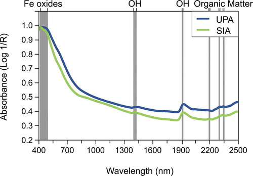
Figure 3 shows average spectral signatures of the two data sets. Generally, the spectra display similar trends and features, with the most pronounced peak around 470 nm indicating the presence of iron oxides (Hunt 1977), two less pronounced peaks at 1,400 nm and 1,900 nm indicating the presence of OH molecules (Hunt 1977), and a number of small peaks at 2,180, 2,306, and 2347 nm that have been previously associated with organic matter (OM; Ben-Dor, Inbar, and Chen 1997; Daniel, Tripathi, and Honda 2003; Stenberg et al. 2010). It is notable that the SIA data set had lower absorbance over the entire spectra region (Figure 3, green line) compared to the UPA data set (Figure 3, blue line). This is most probably due to the lower SOC content in the SIA compared to the UPA (Table 1). Soils with lower SOC content often appear brighter in soil color and generally absorb less light than darker soils with higher SOC concentrations (Stenberg et al. 2010). In the visible part of the spectra (between 400 and 500 nm), a slight concave shape can be observed for the SIA data (Figure 3, green line). The concave shape may indicate larger fraction of clay dominated by iron oxides (Stenberg et al. 2010).

Figure 3. Mean spectra of the complete vis-NIRS data set from Upernaviarsuk (UPA) and Søndre Igaliku (SIA).

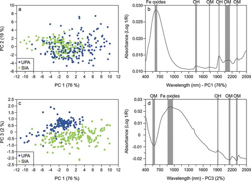
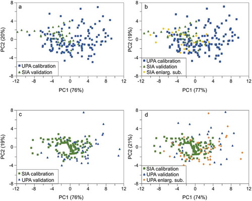
A compositional difference in the investigated soils between and within the investigated sites is presented in Figure 4 with scores and loadings of the computed PCA. The variation in spectral signatures between the two data sets can be explained with the first three PCs, with PC1 explaining 76 percent of the variation within the data set, PC2 19 percent, and PC3 2 percent. In Figure 4a a trend along PC1 is observed, with SIA spectral signatures (green dots) dominating the negative side of PC1 and UPA signatures (blue dots) prevailing on the positive side of PC1, in addition to a great majority of the samples overlapping in the center of the plot. The PC1 loading plot (Figure 4b) may provide an explanation of the differentiation between the two data sets along PC1. Here, we can observe a high positive loading at 620 nm, indicating the presence of iron oxides (Stenberg et al. 2010), a number of smaller peaks—for example, at 1,454 nm indicating OH molecules (Hunt 1977) and at 1930 nm indicating carboxylic acid (Clark et al. 1990)— and two peaks at about 2,100 nm and 2,306 nm both indicating the presence of OM (Ben-Dor, Inbar, and Chen 1997; Stenberg et al. 2010). No clustering of the two data sets was observed along PC2, but there was distinct grouping of the two individual data sets along PC3 (Figure 4c). PC3 explained only 2 percent of the variability within the data set; however, its loadings (Figure 4d) are associated with a large negative peak between 570 nm and 700 nm indicating OM (Galvao and Vitorello 1998) and two smaller negative peaks at 2,100 nm and 2,309 nm also associated with OM (Ben-Dor, Inbar, and Chen 1997). Finally, a broad peak at about 920 nm was observed on PC3 loading (Figure 4d), which could be associated with the presence of iron oxides (Sherman and Waite 1985). The presented results imply that the main variability between the UPA and SIA data sets is in the quantity and composition of iron oxides and organic matter comprising the matrix of the investigated soils.

Figure 4. Principal component analysis of the investigated vis-NIRS data sets reported in scores (a) and (c) and plot of PC1 (b) and PC3 (d) ladings.

Calibration results

The statistics for the optimal calibration models are shown in Table 2. A small number of factors (four to six) and high R² values (always above 0.83) show that the calibration models used in this study are consistent and reliable. The RMSECV values for Models 1 and 2 were reasonably low; however, the RMSECV increased by factor 4 in Models 2.1 and 2.2 (enlarged calibration models). This was due to a broader range of SOC values in these two models, introduced by the UPA enlargement subset.

Table 2. Calibration statistics for the optimal calibration models used in this study.

Model	Pretreatment	Number of factors	R^2	RMSECV
Model 1	2nd SG, 20 s.p.	4	0.94	2.24
Model 2	2nd SG, 20 s.p.	4	0.89	0.51
Model 1.1	2nd SG, 20 s.p.	4	0.92	2.45
Model 1.2	2nd SG, 20 s.p.	4	0.92	2.46
Model 2.1	2nd SG, 20 s.p.	5	0.90	2.18
Model 2.2	2nd SG, 20 s.p.	6	0.83	2.26

RMSECV = root mean squared error of cross-validation; 2^nd SG = second Savitzky-Golay derivative; s.p. = smoothing points.

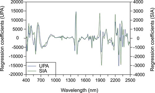
Regression coefficients

The regression coefficients for calibration Model 1 (UPA) and Model 2 (SIA) on the second Savitzky-Golay derivative–transformed spectra are shown in Figure 5. Generally, the regression coefficients had very similar absorption peaks, though they were less pronounced for Model 2 than Model 1. The regression coefficients related to soil organic matter for both sites were located between 570 nm and 700 nm, near 1,660 nm, between 1,700 nm and 1,800 nm, and around 1,900 nm, 2,200 nm, 2,309 nm, and 2,344 nm (Figure 5). Absorption peaks at 1,454 nm and 1,874 nm identify the presence of OH molecules.

Figure 5. Regression coefficients on the Upernaviarsuk and Søndre Igaliku calibration model vis-NIRS data set.

Independent validation of calibration models

Site-specific validation of Models 1 and 2

The site-specific validation (calibration and validation samples from the same area) of Model 1 (UPA) and Model 2 (SIA) is shown in Figures 6a and 6b. Generally, the site-specific validation of SOC calibration models yielded successful predictions, with R² of 0.95 and RMSEP of 1.80 percent for Model 1 and R² of 0.82 and RMSEP of 0.64 percent for Model 2. Higher RPD and RPIQ values (4.74 and 5.31, respectively) were reported for Model 1 than for Model 2 (1.83 and 2.08, respectively). These differences may be associated with the differences in observed SDs and SOC ranges between the two sites, which were higher for the UPA calibration data set (9.1 percent and 0.6 percent–40.9 percent, respectively) than for the SIA calibration data set (1.6 percent and 0.3 percent–9.8 percent, respectively; Table 1). Several studies have argued that a large range in the studied quantities may improve model predictions, due to a larger number of variables defining the spectral reflectance (Stenberg et al. 2010; Bellon-Maurel and McBratney 2011; Gogé et al. 2012). Our results agree with this hypothesis. Another reason for the contrast in model performance could be due to different size of the study areas and sampling density. The UPA is approximately six times smaller compared to the SIA and it was more densely sampled (approximately thirty-five samples/km²), whereas the SIA samples were clustered according to different land uses, with a much smaller average sampling density (less than one sample/km²). Because chemometric modeling is an empirical approach that relies on a similarity between the calibration and validation data sets, the presented results indicate that the UPA samples were more similar to each other regarding the soil composition detected by vis-NIRS compared to the SIA samples. This hypothesis is based only on field observations and results from vis-NIR spectra. Further analysis involving particle size analysis, a complete chemical and mineral composition of soils, etc., is necessary to fully support this theory.

Figure 6. Independent validation of calibration Model 1 (Upernaviarsuk) and Model 2 (Søndre Igaliku).

Site-wise validation of Models 1 and 2

The correlation coefficients generated by Model 1 (Figure 6d) and Model 2 (Figure 6c) for the site-wise validation (calibration and validation samples from different areas) were reasonably high (R² = 0.78 and R² = 0.90, respectively); however, RMSEP was largely increased for both models—for Model 1 by 1.6 times and for Model 2 by 11 times—compared to site-specific validation. Increased RMSEP results in decreased RPD and RPIQ values, indicating poorer model prediction ability. A large increase in bias by a factor of seventeen can be observed for Model 2. Increased bias and thus inaccuracy of the site-wise validation results can be attributed to the heterogeneity of sample origin and the fact that the validation samples were too different from the calibration samples.

Soils in the investigated regions formed on similar two-layered parent material—that is, glacial till and sandy loess—however, the thickness of the eolian sediment varies across the landscape from over 1 m in the SIA to only a couple of centimeters in the outer coastal regions (Jakobsen 1991a). In the UPA, coarse-textured glacial till lies at 0.5 m depth or less, covered by a very thin (~1–2 cm) sandy loess. In contrast, we found very deep and well-developed soil profiles in wind-sheltered valleys in the SIA, as well as less developed soils at elevated sites (646 m.a.s.l.) southwest of Søndre Igaliku. These field observations together with more pronounced soil erosion in the SIA (Fredskild 1992) can partly explain the difference in vis-NIRS model performance between the two study areas. From the two soil profiles described by Jacobsen (1987) for the SIA and Jakobsen (1989) for the UPA, it is apparent that soil texture in the SIA profile is characterized as sandy loam, whereas soil texture in the UPA profile is described as silty loam. The differences in soil texture might have an effect on SOC accumulation within the soil matrix as well as on vis-NIRS modeling. Generally, a dominant sand fraction in soil samples causes more scatter in vis-NIRS spectra, which results in poorer SOC concentration prediction (Stevens et al. 2013). This is consistent with the presented results.

Our study illustrates that vis-NIRS for the prediction of SOC from sites that are geographically and climatically different from the area of soil sampling remains challenging. Although the UPA data set covers a generally large range of SOC values, it does not span the very low values of SOC in the SIA site. The SIA calibration data set covers only low SOC values (Q3 = 2.41 percent); therefore, the local SIA model cannot sufficiently represent the entire UPA data set (Q3 = 12.19 percent). Furthermore, the quality of the SOC estimations from these two data sets most likely varies due to larger fine dust depositions in the SIA area, which is blown out of the glaciofluvial plains in the vicinity of the ice sheet (as presented by Jacobsen (1987). The dust contains small amounts of nutrients that will improve the water-holding capacity of the soils.

Calibration model enlargement

When enlarging calibration models, we first studied the effect of the selection technique to define an enlargement subset added to the computed calibration models. We compared an enlargement subset selected by a Kennard-Stone algorithm with an automated selection of every fourth sample, while ensuring that the extremes were included in each subset. Table 1 shows the main statistical parameters of the enlarged data sets (Models 1.1, 1.2, 2.1, and 2.2). A negligible difference (<1 percent) was observed between the mean SOC (%) values of Models 1.1 and 1.2, whereas a larger difference of 13 percent was observed between the mean values of Models 2.1 and 2.2. The difference is a result of the few samples with higher SOC contents added from the UPA subset. The results of the calibration model performance of all four enlarged models are given in Table 2. The two selection techniques do not play a major role in model performance: the difference in RMSECV for Models 1.1 and 1.2 is negligible (<1 percent), and the difference in RMSECV for Models 2.1 and 2.2 is also very small (3 percent). We would like to emphasize that the size of an enlargement data set can have a significant influence on the results and model performance, as shown in previous studies (e.g., Guerrero et al. 2010; Guy, Siciliano, and Lamb 2015). Small subsets integrate spectral characteristics more easily into the calibration model and therefore improve the model performance (Guerrero et al. 2010). However, Guy, Siciliano, and Lamb (2015) showed that subsets that are too small can be statistically seen as outliers rather than bringing any relevant information to the calibration model. A value of 25 percent proved to result in a good representation of the enlargement resulted, which is apparent in Figures 8b and 8d, where the enlargement subsets efficiently cover the designated PC space.

Below we present independent validation results of calibration models enlarged with samples selected by SOC values (i.e., Model 1.2 [UPA + 25 percent SIA] and Model 2.2 [SIA + 25 percent UPA]). The complete set of site-wise validation results of the enlarged models is provided in Table A1 (see Appendix).

Site-specific validation of enlarged calibration models

The site-specific validation of an enlarged Model 1.2 (Figure 7a) and Model 2.2 (Figure 7b) shows validation statistics (i.e., R², RMSEP, RPIQ) comparable to those of the nonenlarged models presented in Figure 6a (Model 1) and Figure 6b (Model 2). However, the site-specific validation of Model 2.2 generated eight times lower bias compared to the site-specific validation of Model 2. The decrease in bias can be attributed to the enlarged range of SOC values with the introduction of additional UPA samples to the SIA calibration data set. The addition of the UPA subset increased the Q3 value from 2.41 percent SOC (Model 2) to 3.15 percent SOC (Model 2.2; Table 1). This range modification for the SIA data set caused a number of negative predictions for some of the SIA samples with the lowest SOC (Figures 7b and 7d). The RPD and RPIQ values for the site-specific validation of Model 1.2 (Figure 7a) are reasonably high (4.16 and 4.66) and, together with the rest of the presented statistics (R² = 0.94, RMSEP = 2.05, bias = −0.14), indicate a high prediction ability of Model 1.2. This is not the case for the site-specific validation of Model 2.2, where the RPD and RPIQ values are low (0.94 and 1.06, respectively), indicating an unreliable model prediction (Chang and Laird 2002).

Figure 7. Independent validation of the enlarged calibration models when using selection according to soil organic carbon values for enlargement.

Site-wise validation of enlarged calibration models

The prediction ability of the enlarged Model 1.2 (Figure 7d) validated site-wise did not change much compared to the Model 1 (Figure 6d). The R² value was moderate at 0.77, the RMSEP was 2.14, and the RPD and RPIQ were still very low (0.55 and 0.62, respectively). The only notable difference was a decrease in bias, which was sixteen times lower after the enlargement. On the other hand, the enlarged Model 2.2 performance increased significantly, with R² increasing by 5 percent, RMSEP decreasing by 72 percent, and bias decreasing from −4.13 to 0.06. RPD and RPIQ values increased to 4.20 and 4.70, indicating successful prediction.

Enlarging a calibration data set had the most pronounced effect on the site-wise prediction of the SIA validation data set using the UPA calibration model enlarged with 25 percent of samples from the SIA (Figure 7c). To investigate reasons why this technique did not improve prediction ability across both study areas (Model 1.2 and Model 2.2), we studied how the samples from the calibration and validation data sets were situated in the PC space (Figure 8). Adding the subset of SIA samples to the UPA calibration set (Figure 8b) did not seem to significantly expand the SIA set’s variability in the spectral space in comparison to the UPA set before the enlargement (Figure 8a). Thus, the prediction of SOC for the enlarged UPA data set could only be slightly improved (Figure 7d). A contrasting image can be seen in Figure 8c for Model 2. The UPA enlargement subset very efficiently represents the UPA samples, extending the spatial coverage of the SIA calibration set to that of UPA validation set (Figure 8d). The result is a significant increase in performance of the site-wise validation of the enlarged SIA calibration model (Model 2.2; Figure 7c).

Figure 8. Principal component analysis results to support model performance.

Our results show that increasing a range of measurements for a single soil property (e.g., SOC concentration) does not always result in successful predictions. It is well accepted that a number of soil characteristics contribute to the soil matrix and influence soil vis-NIR spectra, such as the presence of iron oxides, mineral composition, quantity and quality of organic matter, soil texture, etc. Building a calibration data set that efficiently covers the main components of subarctic soils is of profound importance and should be addressed in the near future for an efficient application of vis-NIRS in less-accessible environments such as Subarctic Greenland.

Conclusion

This is the first study applying vis-NIRS spectroscopy to investigate concentrations of SOC over a wider area in South Greenland. We determined the predictability of SOC concentrations (%) with vis-NIRS in two climatically distinct subarctic areas, which, due to their variability, could be representative of the soil organic carbon across broader subarctic regions. Our results show that vis-NIRS can successfully predict SOC concentrations in a site-specific application where the soil formation factors are homogeneous and if a large range of SOC measurements is included in the data set. This can reduce exploration costs in remote arctic areas when SOC stocks are evaluated and is of profound importance in areas where combined field sampling, expensive analytical approaches, and remote/satellite data have this far been the main source of soil information for large-scale arctic SOC data sets.

Vis-NIRS predictions might still present a challenge for site-wise application where the target soils greatly differ from the soils used in the calibration data set. Soil development and composition have a large impact on soil spectra and thus the predictive ability of the calibration models. This can be partly overcome by enlarging a calibration data set with a number of local samples from the target location. Yet, this does not always result in successful predictions, as shown in the present study, and the possible reasons should be further investigated. To be able to successfully apply vis-NIRS across different regions, a sufficiently diverse reference database from geographically contrasting areas in the Arctic is needed as input to vis-NIRS calibration models. The development of an international and publicly accessible soil database including vis-NIR spectra and SOC calibration models would greatly reduce exploration costs in remote subarctic and arctic areas. Furthermore, an uncertainty remains in applying vis-NIRS for determination of soil bulk density and soil depth to convert the SOC concentration to estimates of a carbon stock. Future efforts should be made toward the application of vis-NIRS to address at least two environmental problems in these large and so far underresearched regions. Firstly, recognizing small-scale variability of SOC concentration would reduce the large uncertainties in SOC stock calculations. Secondly, a determination of a complete soil matrix with a single vis-NIR measurement could greatly contribute to future exploration for agricultural development of these regions.

Acknowledgments

The authors thank Lasantha Herath, Cecilie Hermanssen, Rene Larsen, Trine Nørgaard, and Stig Rasmussen for assistance in the field; Hans Kapel and Adala Lund for logistical support; the Greenlandic Agricultural Consulting Service (Nunalerinermik Siunnersorteqarfik) in Qaqortoq and Upernaviarsuk for access to the land and their equipment; Bjarne Holm Jakobsen for providing background soil data and insightful discussions for this study; and Bente Rasmussen for laboratory assistance. Finally, the authors would like to thank Jacob Yde and other anonymous reviewers for their constructive comments which improved the paper.

Supplemental data

Supplemental data for this article can be accessed on the publisher’s website.

Disclosure statement

No potential conflict of interest was reported by the authors.

Additional information

Funding

This research was partly funded by a research grant (AUFF-E-2016-9-36) from the Aarhus University Forskningsfond and the research project “Glacial Flour as New, Climate-Positive Technology for Sustainable Agriculture in Greenland: NewLand,” funded by the Independent Research Fund Denmark.

Appendix

Table A1. Independent validation model statistics.

Model	R^2	RMSEP	Bias	SD	IQ	RPD	RPIQ
Model 1 site-specific	0.95	1.8	−0.12	8.53	9.55	4.74	5.31
Model 1 site-wise	0.78	2.82	−0.83	1.17	1.33	2.00	0.47
Model 2 site-specific	0.82	0.64	0.24	1.17	1.33	1.83	2.08
Model 2 site-wise	0.9	7.13	−4.13	8.53	9.55	1.20	1.34
Model 1.1 site-specific	0.95	1.81	−0.25	8.53	9.55	4.71	5.28
Model 1.1 site-wise	0.78	2.83	−0.34	1.17	1.33	0.41	0.47
Model 1.2 site-specific	0.94	2.05	−0.14	8.53	9.55	4.16	4.66
Model 1.2 site-wise	0.77	2.14	0.05	1.17	1.33	0.55	0.62
Model 2.1 site-specific	0.67	1.56	0.35	1.17	1.33	0.75	0.85
Model 2.1 site-wise	0.94	2.01	−0.64	8.53	9.55	4.24	4.75
Model 2.2 site-specific	0.7	1.25	0.03	1.17	1.33	0.94	1.06
Model 2.2 site-wise	0.95	2.03	0.06	8.53	9.55	4.20	4.70

Note that Models 1.1 and 2.1 were enlarged with a subset selected by the Kennard-Stone algorithm and Models 1.2 and 2.2 with a subset selected according to reference SOC values. RMSEP = root mean square error of prediction; IQ = interquartile distance; RPD = ratio of standard error of prediction to standard deviation; RPIQ = ratio of performance to interquartile distance.

References

- Banerjee, S., A. Bedard-Haughn, B. C. Si, and S. D. Siciliano. 2011. Soil spatial dependence in three Arctic ecosystems. Soil Science Society of America Journal 75 (2):591–94. doi:10.2136/sssaj2010.0220.
- Batjes, N. H. 1996. Total carbon and nitrogen in the soils of the world. European Journal of Soil Science 47 (2):151–63. doi:10.1111/j.1365-2389.1996.tb01386.x.
- Bellon-Maurel, V., and A. McBratney. 2011. Near-Infrared (NIR) and Mid-Infrared (MIR) spectroscopic techniques for assessing the amount of carbon stock in soils – critical review and research perspectives. Soil Biology and Biochemistry 43 (7):1398–410. doi:10.1016/j.soilbio.2011.02.019.
- Ben-Dor, E., Y. Inbar, and Y. Chen. 1997. The reflectance spectra of organic matter in the visible near-infrared and short wave infrared region (400–2500 nm) during a controlled decomposition process. Remote Sensing of Environment 61 (1):1–15. doi:10.1016/S0034-4257(96)00120-4.
- Bokobza, L. 1998. Near infrared spectroscopy. Journal of Near Infrared Spectroscopy 6 (1):3–17. doi:10.1255/jnirs.116.
- Burnham, J. H., and R. S. Sletten. 2010. Spatial distribution of soil organic carbon in northwest Greenland and underestimates of high Arctic carbon stores. Global Biogeochemical Cycles 24 (3). doi: 10.1029/2009GB003660.
- Campeau, A. B., P. M. Lafleur, and E. R. Humphreys. 2014. Landscape-scale variability in soil organic carbon storage in the central Canadian Arctic. Canadian Journal of Soil Science 94 (4):477–88. doi:10.4141/cjss-2014-018.
- Cappelen, J. 2011. DMI monthly climate data collection 1768–2010, Denmark, The Faroe Islands and Greenland. Technical 11–05, Danish Meteorological Institute, Copenhagen.
- Chang, C.-W., and D. A. Laird. 2002. Near-infrared reflectance spectroscopic analysis of soil C and N. Soil Science 167 (2):110–16. doi:10.1097/00010694-200202000-00003.
- Clark, R. N., T. V. V. King, M. Klejwa, G. A. Swayze, and N. Vergo. 1990. High spectral resolution reflectance spectroscopy of minerals. Journal of Geophysical Research: Solid Earth 95 (B8):12653–80. doi:10.1029/JB095iB08p12653.
- Daniel, K. W., N. K. Tripathi, and K. Honda. 2003. Artificial neural network analysis of laboratory and in situ spectra for the estimation of macronutrients in soils of Lop Buri (Thailand). Soil Research 41 (1):47–59. doi:10.1071/sr02027.
- Fredskild, B. 1992. Erosion and vegetational changes in South Greenland caused by agriculture. Geografisk Tidsskrift-Danish Journal of Geography 92 (1):14–21. doi:10.1080/00167223.1992.10649310.
- Galvao, L. S., and I. Vitorello. 1998. Role of organic matter in obliterating the effects of iron on spectral reflectance and colour of Brazilian tropical soils. International Journal of Remote Sensing 19 (10):1969–79. doi:10.1080/014311698215090.
- Geladi, P., and B. R. Kowalski. 1986. Partial least-squares regression: A tutorial. Analytica Chimica Acta 185:1–17. doi:10.1016/0003-2670(86)80028-9.
- Gogé, F., R. Joffre, C. Jolivet, I. Ross, and L. Ranjard. 2012. Optimization criteria in sample selection step of local regression for quantitative analysis of large soil NIRS database. Chemometrics and Intelligent Laboratory Systems 110 (1):168–76. doi:10.1016/j.chemolab.2011.11.003.
- Guerrero, C., R. Zornoza, I. Gómez, and J. Mataix-Beneyto. 2010. Spiking of NIR regional models using samples from target sites: Effect of model size on prediction accuracy. Geoderma, Diffuse reflectance spectroscopy in soil science and land resource assessment 158 (1):66–77. doi:10.1016/j.geoderma.2009.12.021.
- Guy, A. L., S. D. Siciliano, and E. G. Lamb. 2015. Spiking regional Vis-NIR calibration models with local samples to predict soil organic carbon in two High Arctic polar deserts using a Vis-NIR probe. Canadian Journal of Soil Science 95 (3):237–49. doi:10.4141/cjss-2015-004.
- Hoffmann, U., T. Hoffmann, E. A. Johnson, and N. J. Kuhn. 2014. Assessment of variability and uncertainty of soil organic carbon in a mountainous boreal forest (Canadian Rocky Mountains, Alberta). CATENA 113:107–21. doi:10.1016/j.catena.2013.09.009.
- Hoffmann, U., T. Hoffmann, G. Jurasinski, S. Glatzel, and N. J. Kuhn. 2014. Assessing the spatial variability of soil organic carbon stocks in an alpine setting (Grindelwald, Swiss Alps). Geoderma 232–234:270–83. doi:10.1016/j.geoderma.2014.04.038.
- Hugelius, G., P. Kuhry, C. Tarnocai, and T. Virtanen. 2010. Soil organic carbon pools in a periglacial landscape: A case study from the central Canadian Arctic. Permafrost and Periglacial Processes 21 (1):16–29. doi:10.1002/ppp.677.
- Hunt, G. 1977. Spectral signatures of particulate minerals in the visible and near infrared. Geophysics 42 (3):501–13. doi:10.1190/1.1440721.
- IPCC. 2014. Climate Change 2014: Synthesis Report. Contribution of Working Groups I, II and III to the Fifth Assessment Report of the Intergovernmental Panel on Climate Change [Core Writing Team, R.K. Pachauri and L.A. Meyer (eds.)]. Geneva, Switzerland: IPCC, 151 pp.
- Jacobsen, N. K. 1987. Studies on soils and potential for soil erosion in the sheep farming area of South Greenland. Arctic and Alpine Research 19 (4):498–507. doi:10.1080/00040851.1987.12002632.
- Jacobsen, N. K., and B. H. Jakobsen. 1986. C14 datering af en fossil overfladehorisont ved Igaliku Kujalleq, Sydgrønland, set i relation til nordboernes landnam. Geografisk Tidsskrift-Danish Journal of Geography 86 (1):74–77. doi:10.1080/00167223.1986.10649230.
- Jakobsen, B. H. 1989. Evidence for translocations into the B Horizon of a Subarctic Podzol in Greenland. Geoderma 45 (1):3–17. doi:10.1016/0016-7061(89)90053-0.
- Jakobsen, B. H. 1991a. Multiple processes in the formation of subarctic Podzols in Greenland. Soil Science 125 (6):414–26. doi:10.1097/00010694-199112000-00003.
- Jakobsen, B. H. 1991b. Soil resources and soil erosion in the Norse settlement area of Østerbygden in Southern Greenland. Acta Borealia 8 (1):56–68. doi:10.1080/08003839108580399.
- Kennard, R. W., and L. A. Stone. 1969. Computer aided design of experiments. Technometrics 11 (1):137–48. doi:10.1080/00401706.1969.10490666.
- Kuhry, P., G. G. Mazhitova, P.-A. Forest, S. V. Deneva, T. Virtanen, and S. Kultti. 2002. Upscaling soil organic carbon estimates for the Usa Basin (Northeast European Russia) using GIS-based landcover and soil classification schemes. Geografisk Tidsskrift-Danish Journal of Geography 102 (1):11–25. doi:10.1080/00167223.2002.10649462.
- Lal, R. 2004. Soil carbon sequestration impacts on global climate change and food security. Science 304 (5677):1623–27. doi:10.1126/science.1097396.
- Malley, D. F., P. D. Martin, and E. Ben-Dor. 2004. Application in analysis of soils. Near-Infrared Spectroscopy in Agriculture 729–84. doi:10.2134/agronmonogr44.c26.
- Massa, C., V. Bichet, É. Gauthier, B. B. Perren, O. Mathieu, C. Petit, F. Monna, J. Giraudeau, R. Losno, and H. Richard. 2012. A 2500 year record of natural and anthropogenic soil erosion in South Greenland. Quaternary Science Reviews 32:119–30. doi:10.1016/j.quascirev.2011.11.014.
- McGuire, A. D., L. G. Anderson, T. R. Christensen, S. Dallimore, L. Guo, D. J. Hayes, M. Heimann, T. D. Lorenson, R. W. Macdonald, and N. Roulet. 2009. Sensitivity of the carbon cycle in the Arctic to climate change. Ecological Monographs 79 (4):523–55. doi:10.1890/08-2025.1.
- Nelson, D. W., and L. E. Sommers. 1996. Total Carbon, Organic Carbon, and Organic Matter. In Methods of Soil Analysis. Part 3 - Chemical methods, SSSA Book Series No. 5, eds. D. L. Sparks et al., 961–1010. Madison, WI: SSSA and ASA.
- O’Rourke, S. M., and N. M. Holden. 2011. Optical sensing and chemometric analysis of soil organic carbon – A cost effective alternative to conventional laboratory methods? Soil Use and Management 27 (2):143–55. doi:10.1111/j.1475-2743.2011.00337.x.
- Palmtag, J., G. Hugelius, N. Lashchinskiy, M. P. Tamstorf, A. Richter, B. Elberling, and P. Kuhry. 2015. Storage, landscape distribution, and burial history of soil organic matter in contrasting areas of continuous permafrost. Arctic, Antarctic, and Alpine Research 47 (1):71–88. doi:10.1657/AAAR0014-027.
- Peng, Y., X. Xiong, K. Adhikari, M. Knadel, S. Grunwald, and M. H. Greve. 2015. Modeling soil organic carbon at regional scale by combining multi-spectral images with laboratory spectra. PLoS One 10 (11):e0142295. doi:10.1371/journal.pone.0142295.
- Post, W. M., W. R. Emanuel, P. J. Zinke, and A. G. Stangenberger. 1982. Soil carbon pools and world life zones. Nature 298 (5870):156–59. doi:10.1038/298156a0.
- Rinnan, R., and Å. Rinnan. 2007. Application of near infrared reflectance (NIR) and fluorescence spectroscopy to analysis of microbiological and chemical properties of arctic soil. Soil Biology and Biochemistry 39 (7):1664–73. doi:10.1016/j.soilbio.2007.01.022.
- Sankey, J. B., D. J. Brown, M. L. Bernard, and R. L. Lawrence. 2008. Comparing local vs. global visible and near-Infrared (VisNIR) diffuse reflectance spectroscopy (DRS) calibrations for the prediction of soil clay, organic C and inorganic C. Geoderma 148 (2):149–58. doi:10.1016/j.geoderma.2008.09.019.
- Savitzky, A., and J. E. M. Golay. 1964. Smoothing and differentiation of data by simplified least squares procedures. ACS Publications. Analytical Chemistry 36 (8):1627–38. doi:10.1021/ac60214a047.
- Scharlemann, J. P. W., E. V. J. Tanner, R. Hiederer, and V. Kapos. 2014. Global soil carbon: Understanding and managing the largest terrestrial carbon pool. Carbon Management 5 (1):81–91. doi:10.4155/cmt.13.77.
- Schumacher, B. 2002. Methods for determination of total organic carbon (TOC) in soils and sediments. Las Vegas, NV: US EPA, Environmental Sciences Division National Exposure Research Laboratory, Office of Research and Development.
- Serreze, M. C., and J. A. Francis. 2006. The Arctic amplification debate. Climatic Change 76 (3):241–64. doi:10.1007/s10584-005-9017-y.
- Shepherd, K. D., and M. G. Walsh. 2002. Development of reflectance spectral libraries for characterization of soil properties. Soil Science Society of America Journal 66 (3):988–98. doi:10.2136/sssaj2002.9880.
- Sherman, D. M., and T. D. Waite. 1985. Electronic spectra of Fe3+ oxides and oxide hydroxides in the near IR to near UV. American Mineralogist 70 (11–12):8.
- Sjöström, M., S. Wold, W. Lindberg, J.-Å. Persson, and H. Martens. 1983. A multivariate calibration problem in analytical chemistry solved by partial least-squares models in latent variables. Analytica Chimica Acta 150:61–70. doi:10.1016/S0003-2670(00)85460-4.
- Sørensen, H., and T. Andersen. 2006. Geological guide South Greenland: The Narsarsuaq-Narsaq-Qaqortoq region. Copenhagen: GEUS, Geological Survey of Denmark and Greenland.
- Sørensen, L. K., and S. Dalsgaard. 2005. Determination of clay and other soil properties by near infrared spectroscopy. Soil Science Society of America Journal 69 (1):159. doi:10.2136/sssaj2005.0159.
- Soriano-Disla, J. M., L. J. Janik, R. A. V. Rossel, L. M. Macdonald, and M. J. McLaughlin. 2014. The performance of visible, near-, and mid-infrared reflectance spectroscopy for prediction of soil physical, chemical, and biological properties. Applied Spectroscopy Reviews 49 (2):139–86. doi:10.1080/05704928.2013.811081.
- Stenberg, B., R. A. Viscarra Rossel, A. M. Mouazen, and J. Wetterlind. 2010. Visible and near infrared spectroscopy in Soil science. In Advances in agronomy, ed. D. L. Sparks, Vol. 107, 163–215. Burlington: Academic Press. doi:10.1016/S0065-2113(10)07005-7.
- Stevens, A., M. Nocita, G. Tóth, L. Montanarella, and B. Wesemael. 2013. Prediction of soil organic carbon at the European scale by visible and near infrared reflectance spectroscopy. PLoS One 8 (6):e66409. doi:10.1371/journal.pone.0066409.
- Summers, D., M. Lewis, B. Ostendorf, and D. Chittleborough. 2011. Visible near-infrared reflectance spectroscopy as a predictive indicator of soil properties. Ecological Indicators, Spatial Information and Indicators for Sustainable Management of Natural Resources 11 (1):123–31. doi:10.1016/j.ecolind.2009.05.001.
- Tarnocai, C., J. G. Canadell, E. A. G. Schuur, P. Kuhry, G. Mazhitova, and S. Zimov. 2009. Soil organic carbon pools in the northern circumpolar permafrost region. Global Biogeochemical Cycles 23 (2):n/a-n/a. doi:10.1029/2008GB003327.
- Viscarra Rossel, R. A., D. J. J. Walvoort, A. B. McBratney, L. J. Janik, and J. O. Skjemstad. 2006. Visible, near infrared, mid infrared or combined diffuse reflectance spectroscopy for simultaneous assessment of various soil properties. Geoderma 131 (1):59–75. doi:10.1016/j.geoderma.2005.03.007.
- Vohland, M., J. Besold, J. Hill, and H.-C. Fründ. 2011. Comparing different multivariate calibration methods for the determination of soil organic carbon pools with visible to near infrared spectroscopy. Geoderma 166 (1):198–205. doi:10.1016/j.geoderma.2011.08.001.
- Volkan Bilgili, A., H. M. van Es, F. Akbas, A. Durak, and W. D. Hively. 2010. Visible-near infrared reflectance spectroscopy for assessment of soil properties in a semi-arid area of Turkey. Journal of Arid Environments 74 (2):229–38. doi:10.1016/j.jaridenv.2009.08.011.
- Walker, D. A., H. E. Epstein, W. A. Gould, A. M. Kelley, A. N. Kade, J. A. Knudson, W. B. Krantz, G. Michaelson, R. A. Peterson, C.-L. Ping, et al. 2004. Frost-boil ecosystems: Complex interactions between landforms, soils, vegetation and climate. Permafrost and Periglacial Processes 15 (2):171–88. doi:10.1002/ppp.487.