Ground surface temperature variability and permafrost distribution over mountainous terrain in northern Mongolia

ABSTRACT

Permafrost plays an important role in numerous environmental processes at high latitudes and in high mountain areas. The identification of mountain permafrost, particularly in the discontinuous permafrost regions, is challenging due to limited data availability and the high spatial variability of controlling factors. This study focuses on mountain permafrost in a data-scarce environment of northern Mongolia, at the interface between the boreal forest and the dry steppe mid-latitudes. In this region, the ground temperature has been increasing continuously since 2011 and has a high spatial variability due to the distribution of incoming solar radiation, as well as seasonal snow and vegetation cover. We analyzed the effect of these controlling factors to understand the climate–permafrost relationship based on in situ observations. Furthermore, mean ground surface temperature (MGST) was calculated at 30-m resolution to predict permafrost distribution. The calculated MGST, with a root mean square error of ±1.4°C, shows permafrost occurrence on north-facing slopes and at higher elevations and absence on south-facing slopes. Borehole temperature data indicate a serious wildfire-induced permafrost degradation in the region; therefore, special attention should be paid to further investigations on ecosystem resilience and climate change mitigation in this region.

KEYWORDS:

• Mountain permafrost
• surface cover
• solar radiation
• temperature variability
• northern Mongolia

Introduction

Both simulations and field investigations at different locations in the Northern Hemisphere report the intensification of enhanced warming and its effects on high- and mid-latitude permafrost and frozen ground dynamics (Pepin et al. 2015; Biskaborn et al. 2019). Changes in frozen ground have important impacts on the surface energy balance, hydrological cycle, and carbon exchange between the atmosphere and ground surface (Zhang et al. 2005). Therefore, the response of permafrost to climate change is of major concern, but present knowledge is still limited, especially in remote areas where long-term environmental monitoring is scarce (Azócar, Brenning, and Bodin 2017). In Mongolia, the mean annual air temperature has increased by 2.07°C since 1940, with higher intensification over the mountainous regions (Ministry of Environment and Green Development 2014). Such an amplified warming has been found to increase the active layer thickness, eventually leading to permafrost degradation in northern Mongolia (Ishikawa et al. 2018).

Seasonal freezing and thawing total degree days of air and ground surface (FDD_a/s and TDD_a/s) are important factors that reflect changes in the cryosphere (Nelson 2003). These factors have been used to predict seasonally frozen ground and permafrost distribution at regional and global scales (Pepin et al. 2015; Obu et al. 2019). However, for smaller geographic scales, including northern Mongolia, the model outputs have been less accurate due to a lack of precise data sets, such as vegetation and snow cover and microclimatic conditions (Riseborough et al. 2008; Hasler et al. 2015). In mountainous terrain, air temperature, surface characteristics, and radiation balance are major factors in the variability of surface net energy balance (Williams and Smith 1989), as well as the extent of mountain permafrost, especially in semi-arid regions. Several studies have been conducted in the Khuvsgul Mountains of northern Mongolia regarding the distribution of mean ground surface temperature (MGST) to predict the permafrost distribution (Etzelmüller et al. 2006), active layer thickness (Heggem et al. 2006), and thawing n-factor (the ratio between air temperature [T_a] and surface temperature [T_s] during the thawing season) in different land covers (Anarmaa et al. 2007).

In regions with rugged topography, such as Sugnugur catchment in the Khentii Mountains, the distribution and dynamics of permafrost have not been well documented. Permafrost in this catchment plays an important role in the hydrological cycle and acts as an impermeable layer allowing lateral subsurface flow that sustains river discharge during the dry seasons (Kopp, Lange, and Menzel 2016). Therefore, it is important to assess the distribution of permafrost with a high spatial resolution. Negative MGST is a good indicator of permafrost presence over mountain terrains where the thermal properties of soil can differ significantly (Etzelmüller et al. 2006; Luo, Jin, and Bense 2019).

This study focuses on understanding the effects of snow and vegetation cover, potential solar radiation (PSR), and topography on the spatial variability of T_s and calculating MGST over the Sugnugur catchment to predict permafrost distribution with a 30-m resolution. The calculated MGST is validated against observed in situ T_s measurements and borehole data. The results contribute to a better understanding of the temporal and spatial variability of T_s and permafrost occurrence in this rugged mountainous terrain of northern Mongolia.

Study area

The study area is the Sugnugur catchment, which is situated in the discontinuous permafrost region of northern Mongolia at the southern boundary of Eurasian permafrost (Figure 1). Thus, it includes the sensitive transition zone between the steppe and the boreal forest (Kopp, Lange, and Menzel 2016). This catchment generates an essential headwater stream of Kharaa River, which eventually drains into Lake Baikal through Selenga River (Menzel, Hofmann, and Ibisch 2011). Therefore, the seasonal frozen ground and permafrost in the catchment are of ecological and socioeconomic importance for the approximately 147,000 inhabitants living in the Kharaa River basin (Karthe et al. 2014).

Figure 1. Location of the study area, its topography, and the positions of temperature measurement transects across the Sugnugur Valley (indicated by T1–T4; see details in Table 1). The inset shows the PPI (at 1-km resolution), which indicates the likelihood of permafrost existence at a global scale (Obu et al. 2019). The hydroclimatic station (green dot) is situated at 1,193 m.a.s.l. BH = the position of the two boreholes located on the north-facing slope near transect 3

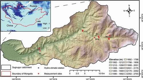
The elevation of the catchment ranges from 1,062 m.a.s.l. to 2,703 m.a.s.l. at the peak of the Khentii Mountains. Sugnugur catchment has rugged topography, with steep south-facing and relatively gentle north-facing slopes. Mean air temperature (MAT) for the last five years is slightly lower than −1°C and mean annual precipitation is about 350 mm (Kopp, Minderlein, and Menzel 2014). In the study area, north-facing slopes are covered by boreal forest with thick moss layers. South-facing slopes are sparsely vegetated, and the valley bottom is dominated by shrubs and short grasses. Since 2009, about one third of the forest cover has been affected by wildfires (Kopp, Lange, and Menzel 2016). Permafrost in northern Mongolia mostly exists on north-facing slopes and is absent on south-facing slopes (Etzelmüller et al. 2006; Ishikawa et al. 2008). Depending on the climatic conditions and surface characteristics, it can also sometimes be found in the valley bottoms. Distinct hydrological behaviors of runoff generation processes on burned (quick flow predominant) and unburned (preferential flow predominant) north-facing slopes are evident in this catchment (Lange et al. 2015). The soil in the shrub-dominated bottom of the valley has relatively high moisture contents throughout the summer months due to interflow from the north-facing slopes (Minderlein and Menzel 2014).

Data and methodology

Data

In situ measurements

Ongoing hydroclimatic observations have been monitored since 2010 at the bottom of the Sugnugur Valley on a permanent monitoring site (referred to as the hydroclimatic station site in this article; Figure 1). More than forty parameters are continuously measured with high temporal resolutions, including the individual radiation components, snow depth, T_s, and T_a (for a detailed list of sensors and parameters, see Minderlein and Menzel 2014). Before our monitoring program started, the study region was lacking any environmental data. We calculated the summer temperature lapse rate (LR) for summers 2011 and 2012 using daily mean T_a data from three temporary climatic stations distributed along the Sugnugur Valley and the permanent hydroclimatic station. T_a was also measured at four locations for 2016–2017 (including complete thawing T_a > 0°C and freezing T_a < 0°C seasons) using temperature measured from iButtons (Maxim integrated) with ±0.25°C accuracy (Way and Lewkowicz 2018). The iButtons were installed in radiation shields and placed 1.5 m above the surface and recorded temperature at 3-hour intervals. The measurement positions included the bottom of the valley and a mountain summit at 2,020 m.a.s.l. Temperature inversions, which frequently occur during winter, were also studied from the iButton measurements.

We also used iButtons to measure T_s at twelve locations at valley transects, in addition to the hydroclimatic station. Measurements were taken at a depth of 5 cm in diverse surface and topographic settings. Two iButtons were operated in parallel at each location in order to prevent any data loss. iButton measurements were evaluated using the T_s record with that of a Campbell 107 temperature probe installed at the same depth at the hydroclimatic station site. The iButtons provided slightly higher temperatures with regard to the standard probe, possibly as a result of a greenhouse effect created by the plastic shelters in which the iButtons were housed. The overall Pearson’s correlation coefficient between the two separate records was r = 0.997, allowing us to calibrate the iButton data with the Campbell 107 temperature probe using a linear regression.

In addition, two boreholes were dug manually in a severely burned forest (SBF, in December 2015) and in an unburned forest (UBF, in September 2016). The boreholes were each equipped with temperature and moisture sensors at depths ranging from 0 to 290 cm for the SBF site and from 0 to 120 cm for the UBF site. Deeper placement of sensors at the UBF site was not possible because we reached the permafrost table at a depth of 120 cm. Temperature data at 5 cm depth were used as an additional validation of MGST. The relative distance between the boreholes is roughly 600 m and both are located on the same north-facing slope. All temperature sensors were connected with HOBO-U12 data loggers; recordings were made at 4-hour intervals. Both iButton and borehole T_s measurement sites are described in Table 1.

Table 1. Descriptions of temperature measurement sites. South-facing slopes with greater inclination receive higher potential potential solar radiation (PSR)

ID	Transect number^a	Temperature measurement	Slope	Elevation (m)	Vegetation type	Aspect	Inclination (°)	PSR (Wm^−2)
1	1	Surface	South	1,281	Sparse vegetation	S	18	182
2		Surface and air	Valley bottom	1,193	Short grassland	SW	9	175
3		Surface	North	1,281	Sparse forest	NW	21	134
4	2	Surface	South	1,393	Sparse vegetation	SW	35	172
5		Surface and air	Valley bottom	1,356	Bare ground	W	4.4	145
6		Surface	North	1,393	Dense forest	NE	22	111
7	3	Surface	South	1,558	Sparse vegetation	S	35	190
8		Surface and air	Valley bottom	1,485	Short grassland	NE	2.8	161
9		Surface	North	1,558	Dense forest	NE	10	149
10		Surface	North	1,560	Dense forest	NE	10	147
11		Surface	North	1,530	Burned forest	N	7	158
12	4	Surface	Valley bottom	1,583	Shrubland	NW	5	148
13		Surface	North	1,612	Sparse forest	NW	14	140
14		Surface and air	Mountain top	2,020	Rock debris	S	8	196

Note: ^aSee Figure 1.

Soil thermal conductivity and biomass measurements were also conducted during the thawing season in September 2017 at all iButton and borehole locations. Soil thermal conductivity was measured at depths of 10, 20, and 40 cm using a Decagon KD2 Pro thermal conductivity meter. Biomass samples were collected from 50 × 50 cm plots and weighed and then dried in an oven at 100°C for approximately 2 hours until the weight stabilized. The late winter accumulated snow depth (ASD) was manually measured during a winter field campaign (in the beginning of March 2017).

Remote sensing data

The spatial distribution of vegetation cover was obtained from the soil-adjusted vegetation index (SAVI; Abramov, Gruber, and Gilichinsky 2008; Boeckli et al. 2012), which was derived from six Landsat images (2012–2017). These images were taken in either July or August, the months assumed to represent peak vegetation cover (Pan et al. 2019). The snow cover area (SCA) over the Sugnugur catchment was derived from forty remote sensing images from Landsat 7 and 8 and Sentinel 2 satellites (Munkhjargal et al. 2019). A digital elevation model (DEM) with 30-m spatial resolution from the Advanced Spaceborne Thermal Emission and Reflection Radiometer (ASTER GDEM 2) was used to derive the spatial variability in T_a.

Methodology

This section describes the different processes in the framework of the applied methodology (Figure 2). First, temperature regime and seasonal n-factors were calculated to understand the permafrost dynamics and the effect of snow and vegetation cover on T_s variability (Lunardini 1978; Smith and Riseborough 1996). We then calculated the spatial variability of MGST for 2016–2017, assuming that negative values can indicate the presence of permafrost. MAT for 2016–2017 was derived from the distribution of PSR and annual LR. Surface offset (SO), which is the difference between MAT and MGST, was calculated from in situ temperature measurements in various topographic settings with seasonal snow and vegetation cover and then added to the MAT to obtain MGST based on the derived SCA and SAVI. To reduce unreasonably high or low values, focal statistics were used for smoothing by averaging the values of the surrounding 3 × 3 pixels. The final MGST was validated using iButton surface temperature measurements at twelve locations and temperature data from the two boreholes near transect 3 (Figure 1) and were also compared to the recently published permafrost probability index (PPI) map by Obu et al. (2019). The equations, parameters, and abbreviations are shown in Table 2.

Table 2. Parameters used in the article and their calculation

No.	Abbreviation	Parameter	Unit	Calculation method
1	FN	Frost number	Unitless	$\frac{\sqrt{\mathrm{F}\mathrm{D}\mathrm{D}\mathrm{a}}}{\sqrt{\mathrm{F}\mathrm{D}\mathrm{D}\mathrm{a}}+\sqrt{\mathrm{T}\mathrm{D}\mathrm{D}\mathrm{a}}}$
2	MAT	Mean annual air temperature	°C	$\mathrm{M}\mathrm{A}\mathrm{T}=\left(\alpha \times \mathrm{P}\mathrm{S}\mathrm{R}+\beta \right)+\mathrm{L}\mathrm{R}$α and β are empirical parameters
3	PSR	Potential solar radiation	Wm^−2	Direct + Diffusive
4	LR	Lapse rate	°C m^−1	Annual air temperature gradient per meter
5	MGST	Mean annual ground surface temperature	°C	(nt × TDDa − nf × FDDa)/365
6	TDDa	Air thawing degree days	°C days	Annual sum of daily air temperatures above 0°C
7	FDDa	Air freezing degree days	°C days	Annual sum of daily air temperatures below 0°C
8	nt	Thawing n-factor	Unitless	TDDs/TDDa
9	nf	Freezing n-factor	Unitless	FDDs/FDDa
10	TDDs	Surface thawing degree days	°C days	Annual sum of daily surface temperatures above 0°C
11	FDDs	Surface freezing degree days	°C days	Annual sum of daily surface temperatures below 0°C
12	SO	Surface offset	°C	MGST − MAT
13	Ta	Ambient air temperature	°C	Observed at 1.5–2 m height
14	Ts	Surface temperature	°C	Observed at 5 cm depth
15	SAVI	Soil adjusted vegetation index	Unitless	$\frac{\mathrm{N}\mathrm{I}\mathrm{R}-\mathrm{R}\mathrm{E}\mathrm{D}}{\left(\mathrm{N}\mathrm{I}\mathrm{R}+\mathrm{R}\mathrm{E}\mathrm{D}+\mathrm{L}\right)}\ast \left(1+\mathrm{L}\right)$L is assumed to be 0.5
16	ASD	Accumulated snow depth	cm	Maximum late winter snow depth
17	LST	Land surface temperature	°C	Derived from Landsat images
18	FT	Discrete Fourier transform	—	Reveals periodicities in input data
19	SBF	Severe burned forest	—	—
20	UBF	Unburned forest	—	—

Figure 2. Flowchart of the methodology

Temperature variability

Temperature regime

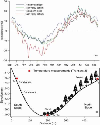
To analyze the effects of topography on T_s, we placed iButtons along transects from the south-facing to the north-facing slopes of the valley, including the valley bottom. In total, four transects (see Figure 1) were developed at different elevations. The surface characteristics and a description of each temperature measurement site are shown in Table 1. The iButtons were positioned at the same elevation on both slopes in each transect to reduce the effect of the adiabatic T_a gradient on T_s. T_a was observed at the bottom of the valley and on the mountain top, above the T_s measurements (Figure 3b). The summer (June–July–August) and winter (December–January–February) LRs were used to derive an annual LR, which was later used as an adjustment factor in the spatial distribution of MAT to 2016–2017. The frost number (FN), which indicates the likelihood of permafrost occurrence, was calculated for all T_a measurement locations (Table 2). The FN ranges from 0 to 1, with a threshold of >0.5 indicating the presence of permafrost at a regional or global scale (Heggem et al. 2006). However, it does not confirm the existence of permafrost, because this cannot be determined without knowing the effects of snow and vegetation covers and the thermal properties of the soil (e.g., Smith and Riseborough 2002). To understand the general temperature regime in this region, the TDD_s for six seasons and FDD_s for seven seasons were also calculated at the hydroclimatic station site.

Figure 3. (a) An example of the temperature variability during the study period and (b) the locations of temperature measurements, typical topography, and land cover in the study region as valley transect. The temperature values are five-day averages

Effect of surface cover

Seasonal snow and vegetation cover insulates the heat flow between the atmosphere and ground surface, resulting in higher during winter and cooler T_s during summer compared to T_a. Snow cover decouples the T_s from T_a due to its low thermal conductivity (Ishikawa 2003; Harris et al. 2009). Using the T_s and T_a measurements at the hydroclimatic station site, we evaluated the interannual variability of the thawing (n_t) and freezing (n_f) n-factors. Furthermore, the relation between biomass and TDD_s was analyzed across the valley transects. The SO was also calculated at four locations where both T_s and T_a exist. The equations can be found in Table 2. The seasonally persistent SCA—that is, the snow that uninterruptedly covers the ground—was analyzed by determining the Normalized Difference Snow Index with a value of >0.4, indicating the presence of snow cover, as recommended by Hall et al. (2002). Based on the SAVI, the study area was classified into vegetated and nonvegetated surfaces. To simplify the variability in SO over the study area, it was assumed to be different for the vegetated and persistent snow cover areas as well as the nonvegetated, mostly rock debris surfaces on steep slopes based on the calculated n-factors.

Regionalization of air temperature

In mountainous regions with strong topographic gradients, incoming solar radiation plays a significant role in the spatial distribution of both T_a and T_s. The relationship between PSR and either T_s or T_a has been studied in permafrost regions (Lacelle et al. 2016). T_a in heterogeneous terrain mainly depends on topography and other microclimate factors such as cloud cover, precipitation, and surface characteristics (Strachan and Daly 2017). Temperature and solar radiation follow similar patterns as they change with time, but variances in temperature lag behind variances in solar radiation. In this study, empirically derived MAT was considered as a good indicator of MGST because T_a usually follows the diurnal variation in T_s due to the reflected radiation from the ground surface (Chou, Sheng, and Zhu 2012). Therefore, we analyzed a five-year time series of incoming solar radiation and T_a data recorded at the hydroclimatic station and found that 30 days of lag is the best fit to remove the time lag between the two variables. Similar time lags were also found and used for modeling temperature in previous studies at both local and global scales (Douglass, Blackman, and Knox 2004; Huang et al. 2008). This suggests that if the study area is assumed to have homogenous atmospheric conditions, T_a can be predicted as a fraction of PSR after a series of adjustments.

Adjustment of T_a includes (1) aggregation of the observed daily values (from transects 2 and 3) to ten-day averages, (2) removal of the variation using discrete Fourier transform (FT), and (3) removal of the thirty-day time lag to improved the correlation with solar radiation. The FT uses two phases, which indicate the absolute values within the annual time series. This results in a smoothing of the T_a by sinusoidal oscillations around the mean value. To meet the time step of the adjusted T_a, PSR was also calculated for a whole year as a ten-day running average using the PSR model using ArcGIS spatial analysis tools (Fu and Rich 2002) and the DEM. The calculation is the sum of direct and diffuse radiation repeated for each feature location or every location on the topographic surface. Then, MAT for 2016–2017 was obtained from the calculated PSR using a linear regression analysis and adding the annual LR with the assumption that a clear sky was homogenous over the study area. The equation is provided in Table 2.

Results and discussion

Temperature regime

Data from the surface temperature iButtons indicate that the freezing season extends from the beginning of October to the end of March at all observed locations, with prolonged periods below 0°C at higher elevations (Munkhjargal et al. 2019). The surface freezing period on north-facing slopes starts a few days earlier and ends later compared to that on south-facing slopes due to extended snow cover, duration of phase change, surface cover, and less incoming radiation. FN values calculated from the observed T_a measurements ranged from 0.5 to 0.6, indicating the potential occurrence of permafrost in the study area (Etzelmüller, Berthling, and Sollid 1998). However, MGST is more sensitive to changes in n-factors, solar radiation, and soil moisture (Heggem et al. 2006; Juliussen and Humlum 2007).

The observed MGST on south-facing slopes was 3–4°C higher than that on north-facing slopes (Figure 3a). The temperature difference between the slopes is more pronounced during the thawing season, especially on hot days with clear skies. Observations of T_a and T_s at the four sites indicate that T_s is initially warmer than T_a at all sites, with notably less fluctuation in winter due to the insulating effect of snow. The difference in T_s between the opposite slopes is the lowest during winter. It increases again in late winter because T_s on the south-facing slope increases rapidly with T_a, whereas T_s on the north-facing slope gradually increases due to the extended snow cover and required latent heat energy to warm the soil during phase change. Therefore, the variability in MGST across the valley is high.

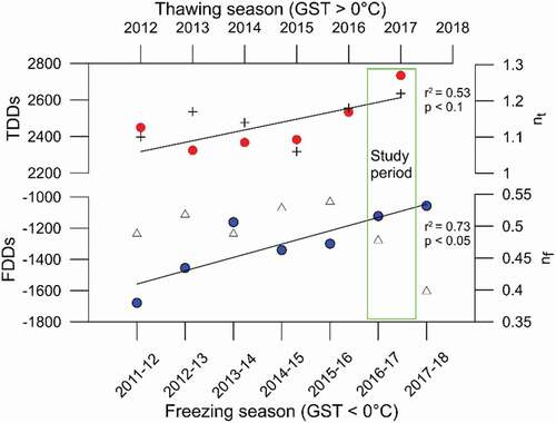
The observed MAT at the hydroclimatic station site was −1.06°C. The study period 2016–2017 was unusually warm with low FDD_s and high TDD_s due to a thicker snowpack in winter and a dry summer, respectively. Moreover, T_s observation revealed a continuous increase in both thawing and freezing seasons over the last seven years (Figure 4) as representative of the general temperature regime in the study area. Unusual wildfire events occurred in the region in summer 2017 as a result of the extreme dryness and increased temperatures. Thus, the continuously increasing T_s may have contributed to the deepening of the active layer, particularly in areas that were seriously affected by wildfires.

Figure 4. Calculated TDD_s and FDD_s at the hydroclimatic station. The study period covers the complete thawing and freezing seasons when the iButton measurements were conducted

We analyzed the relationship between T_s and T_a at different elevations using linear regression analysis. The correlation coefficient (r²) between the two variables decreased as elevation increased (Figure S1, Supplementary material) and can be attributed to the extended snowpack at higher elevations and to slower temperature changes at the ground surface compared to in the air (Peng et al. 2015). Strong seasonal variability in T_a exists in the study area as well, as indicated by the mean summer LR of −0.011°C m⁻¹ (found from the four climate stations) and winter inversion of 0.006°C m⁻¹. Nevertheless, the annual LR was found to be −0.005°C m⁻¹, or similar to the commonly accepted environmental LR of −0.006°C m⁻¹ (Minder, Mote, and Lundquist 2010).

Effect of surface covers

Surface covers as insulating materials

To analyze the influence of the snow cover on T_s, the snow depth observed at the hydroclimatic station was examined in conjunction with other corresponding parameters (Table 3). The seasonally persistent snow cover lasts about 130–140 days from early November to late March, and its duration is substantially longer at higher elevations. The mean insulating effect of seasonal snow cover on T_s, or n_f, was relatively consistent or roughly 0.5 for the last five winters at the hydroclimatic station site (Figure 3).

Table 3. Mean and maximum snow depth (cm) at the hydroclimatic station site, together with ground surface temperature (T_s, °C), air temperature (T_a, °C), and incoming solar radiation (ISR, Wm⁻²) in winters since 2012

	2012–2013	2013–2014	2014–2015	2015–2016	2016–2017	2017–2018
Mean	25	19	12	15	19	—
Maximum	41	26	25	26	29	—
Ts	−10.4	−8.9	−10	−9.8	−8.3	−7.9
Ta	−20.3	−17.2	−16.7	−19.2	−17.4	−16.3
ISR	87.8	96.1	92.3	86.5	95.6	94.2

Note: T_s, T_a, and ISR are the daily mean values between November and March during the period of persistent snow cover.

The development of a seasonal snow cover plays a significant role in the variability in T_s; a gradually weakening insulating effect with increasing snow depth and air temperature toward the end of the freezing season was evident (Figure 5). During this time, T_s became less sensitive to variations in T_a due to the greater snow depth. The low T_s below the snowpack tended to remain for an extended period as a consequence of the low thermal conductivity of snow restricting the loss of heat from the ground.

Figure 5. Calculated n-factors at each transect during the study period. Values greater than 1.0 indicate lower T_s during the freezing season and higher T_s during the thawing season relative to T_a

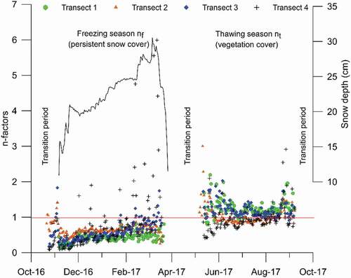
In general, snow depth appears to be independent of elevation based on the field measurements (Table S1, Supplementary material). The percentage of persistent snow cover area throughout winter was 94 percent in the Sugnugur catchment (Munkhjargal et al. 2019). We conclude that n_f is homogenously 0.5 in the areas with persistent snow cover. Steep south-facing slopes were snow-free most of the time due to prevailing winds and relatively high incoming solar radiation, which resulted in snow redistribution and greater sublimation rates, respectively.

Forested north-facing slopes were the richest in biomass, followed by the valley bottom shrublands and sparsely vegetated south-facing slopes. Near transect 3, for instance, a biomass value of 0.07 kg/m² on the south-facing slope, 0.825 kg/m² on the bottom of the valley, and a value of 4.935 kg/m² under dense forest were found. Notably, the amount of biomass in the SBF was 2.430 kg/m⁻², or roughly half that of the UBF; this distinction demonstrates the effects of wildfires on biomass. Yoshikawa et al. (2002) explained the implications of wildfire and reduction in vegetation cover on the ground thermal regime in Interior Alaska. The soil in the SBF showed the highest thermal conductivity due to the reduction in the moss layer and increased water content, which is similar to that found in Interior Alaska (Yoshikawa et al. 2002). The reduced vegetation cover resulted in a higher TDD_s in the SBF compared to the adjacent UBF.

To evaluate the effect of vegetation cover on T_s, we correlated the sampled dry biomass measurements against the surface TDD_s at all T_s measurement sites, except for high-elevation rock debris surfaces (Figure S2, Supplementary material). There was a significant negative relationship between the two variables, indicating that greater biomass protects the underlying surface from summer overheating. The lowest TDD_s values were observed at the valley bottom site near transect 4, which is characterized by dense shrubs located near the Sugnugur riverbank. We speculate that this is probably due to increased soil moisture content, which reduces surface heating as a result of an interrelation between surface and subsurface flows from the north-facing slope and the shading effect of the dense shrubs.

N-factors and surface offset

The relationship between surface and air temperatures has not been previously described for the Khentii Mountains. The seasonal snow-induced freezing n_f was relatively consistent, ranging between 0.5 and 0.6 at all sites, and thawing n_t ranged from 0.8 at the top of the mountain to 1.2 in short grassland at lower elevations (Table 4). The n_t values exceeding 1.0 indicate that T_s was warmer than T_a. Unlike at other sites, T_s at the rock debris surface was lower than T_a, probably due to high albedo resulting in less net radiation. However, other site characteristics such as canopy closure, dryness, and organic layer thickness can also influence this relationship (Karunaratne and Burn 2004). In winter, T_s at all locations was higher than T_a due to the snow insulation effect.

Table 4. Observed surface offset and n-factors at the measurement sites

Transect	SO (°C)	nf	nt	ASD (cm)	SAVI	Surface characteristic	Elevation (m)
1	4	0.52	1.2	24	0.37	Short grassland	1,193
2	3.5	0.6	1.05	20	0.3	Poorly vegetated	1,356
3	4	0.53	1.16	25	0.38	Shrubland	1,485
4	1.5	0.52	0.8	NA	0.08	Rock debris (mountain)	2,020

Note: The annual surface offsets at vegetated sites were relatively similar but differed significantly for rock debris surfaces. The values at transect 1 are the mean of the last five years.

The period with temperature measurements was not long enough to perform a comprehensive evaluation of the interannual variations in the n-factors. Nevertheless, we believe that seasonal n-factors at different elevations and slopes were identified for this region because the annual variations in the n-factors were relatively stable at the hydroclimatic station. Considering the similar n_f and n_t factors except for the rock debris surface, we conclude that SO is +4°C for vegetated and persistent snow cover area and +1.5°C for nonvegetated rock debris surface. These results are in line with Boeckli et al. (2012), who assumed that the SO of the vegetated area is 2°C greater than that of nonvegetated rock debris surfaces in the European Alps, further suggesting that our results are reasonable.

The heat exchange between air and surface varied significantly in early spring and late autumn (the transition periods) when n_f and n_t converge. Therefore, the freezing season n-factors during the transition periods are important components of the overall seasonal n_f. The calculated mid-season n_f values were closest to the seasonal n_f. Like n_f, mid-season n_t values were closest to the seasonal n_t and during that time T_s and T_a were similar (Figure 5). However, the seasonal n_t may depend on the length of the thawing season. Figure 5 illustrates the ratios between daily T_s and T_a in the four transects. Note that calculations were only made for the bottom of the valley and on the mountain top, where both T_a and T_s measurements exist. There were some days with colder T_s than T_a during winter at transects 3 and 4 in the upper valley, which was probably due to the inversion effect.

Anarmaa et al. (2007) studied n_t under various vegetation covers in a valley of the Khuvsgul Mountains in northern Mongolia using a T_a measurement from a single location. This would mean that T_a is constant across the valley and that the only influence on T_s is the overlying vegetation. Such calculation may lead to relatively low n_t on north-facing slopes and high n_t on south-facing slopes. We suggest that T_a can vary at smaller scales depending on both exposure and elevation. Therefore, the variability in T_s across the Sugnugur Valley was considered as a result of the spatial distribution of snow and vegetation cover, incoming solar radiation, topography, and the length of the thawing season.

In addition, we checked the associations between the calculated parameters and MGST at all T_s measurement sites using Pearson’s correlation analysis (Table 5). The parameters include the measured snow and biomass, as well as 30-m gridded data including PSR, elevation, and mean land surface temperature (LST) derived from the Landsat images that were used to retrieve SAVI in this study. To avoid high collinearity, the parameters that require T_a measurement were not considered due to (1) the limited number of T_a measurements in the valley and (2) its strong relationship with T_s. The results show that the spatial distribution of MGST might be better explained by the variability in TDD_s (r = 0.94, p < .01) rather than FDD_s (r = 0.68, p < .05). This indicates that though n_f is relatively consistent over the study area, n_t plays a major role in the variability in MGST over the Sugnugur catchment. Both the PSR and biomass showed statistically significant correlations with MGST. Due to the high temperature differences across the valley transects during hot summer days, we also tested the relationship between the Landsat-derived LST and the corresponding parameters. These results showed significant negative correlations with biomass and elevation and a positive relationship with TDD_s, indicating that the greater the biomass and the higher the elevation, the lower the T_s during the thawing season. The ASD did not show any significant relation with its associated parameters.

Table 5. Pearson’s correlation coefficient (r) matrix between some parameters;

	Elevation	PSR	TDDs	FDDs	Biomass	ASD	LST	MGST
Elevation	1
PSR	0.27	1
TDDs	−0.46	0.60*	1
FDDs	0.04	0.45	0.39	1
Biomass	0.37	−0.65*	−0.8**	−0.21	1
ASD	0.06	−0.34	—	0.17	—	1
LST	−0.69*	0.32	0.78**	0.4	−0.62*	—	1
MGST	−0.35	0.65*	0.94**	0.68*	−0.7*	−0.32	—	1

Note: *p < .05. **p < .01.

Derivation of mean air temperature

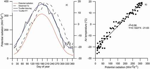
The MAT for 2016–2017 was derived empirically from the PSR and annual LR. Figure 6a illustrates the ten-day running average curves of PSR and T_a. Figure 6b shows the linear regression analysis between the two variables and the obtained regression parameters that were used to calculate MAT over the study area. Following the thirty-day time lag adjustment, the r² increased from 0.76 to 0.96. The result indicates that the distribution of MAT can be improved by considering the influence of incoming solar radiation in addition to the local adiabatic LR. Consequently, the derived MAT showed a significant difference between the north- and south-facing slopes at the same elevations. In a similar landscape, Dashtseren et al. (2014) observed a much lower T_a in a forested north-facing slope in both summer (by 2–3°C) and winter (by 1–2°C) seasons, relative to the opposite south-facing slope. However, the linear relationship with PSR may lead to uncertainties on steep slopes with high inclinations where the incoming radiation is very high or low. Therefore, additional T_a measurements on different slopes, placed at short horizontal distances to minimize the effect of adiabatic air, may reduce the uncertainties.

Figure 6. (a) Distribution curves of ten-day average potential radiation and observed and adjusted air temperatures at transect 3. After time lag and FT adjustments, the variance between potential radiation and temperature was significantly reduced. (b) The linear regression on the right shows the correlation between the adjusted T_a and potential radiation at transects 2 and 3. The linear equation was later applied for the estimation of MAT for 2016–2017

Determination of mean ground surface temperature

MGST was estimated for a one-year period from September 2016 to September 2017, including the complete freezing and thawing seasons. Although the study period was short, we believe that the spatial pattern of MGST and permafrost distribution has been successfully derived (Figure 7). The comparison between the produced permafrost map and the recent MODIS-derived PPI using the temperature on top of permafrost model (Obu et al. 2019) shows overall agreement but with significant disagreement particularly on south-facing slopes. These discrepancies were expected due to the scale difference between the two maps (30 m and 1 km). Most of the T_s measurement sites at each transect, for instance, are within a single 1-km pixel. It is also worth mentioning that the modeled PPI is underestimated in this region because permafrost is covered by forest and moist organic layers, which favor the existence of permafrost (Obu et al. 2019).

Figure 7. Calculated MGST in the Sugnugur catchment for 2016–2017. The PPI lines indicate the permafrost probability index from Obu et al. (2019). The inset shows the relationship between the observed MGST at individual sites and the estimated MGST. Red circles mark the outliers described in the text

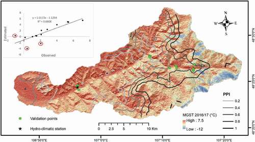
The findings show good agreement with the T_s validation sites (inset in Figure 7), with the exception of a few outliers. In general, south-facing slopes indicate the absence of permafrost (MGST > 0°C), whereas north-facing slopes show the presence of permafrost (MGST < 0°C). The MGST for the study period ranges from +7.5 to −12°C with a root mean square error of ±1.4°C (r² = 0.68). The two outliers with underestimations as much as 3°C represent the sites on strongly inclined north-facing slopes. In contrast, the outlier with an overestimation of 2°C comes from the valley bottom at transect 4, where a mixture of shrub and forest persists with shallow snow cover (only 12 cm). The areas in the valley bottom are mostly shaded by dense shrubs and show a relatively high soil moisture content (Kopp, Minderlein, and Menzel 2014). This may result in high evapotranspiration rates, reduced summer heating, and enhanced winter heat loss, thus favoring the existence of permafrost. We believe that such outliers appear due to the empirical linear relationship between PSR and MAT, as well as the shallow ASD and high moisture content.

Both the estimated MGST and PPI showed the possible existence of permafrost at the two borehole sites on the north-facing slope near transect 3. The calculated MGST in the SBF was 0.34°C (observed value 1.46°C) with a PPI of 0.41, and that in the UBF was −0.21°C (observed value 0.15°C) with a PPI of 0.44. Borehole temperature data between 2016 and 2018 in these two land covers indicate a significant increase in ground temperature in the SBF (Figure S3, Supplementary material). It is important to note that the combination of wildfire and an increased surface temperature in both thawing and freezing seasons over the last seven years may have triggered permafrost degradation in the study area. In addition to the borehole data, electrical resistivity surveys across the valley transects may help to further validate our results and draw a strong conclusion on permafrost distribution.

Conclusions

The distribution of permafrost in mountainous regions is a result of the heat balance between the ground and the air and can be predicted more precisely by determining the effects of vegetation and snow cover, microclimatic conditions, topography, and thermal conductivity of the soil. Based on in situ temperature measurements, we observed an MGST difference of 3–4°C on the north- and south-facing slopes within a short horizontal distance, seasonal T_a variability with elevational gradient including winter inversion, and generally increasing T_s in both freezing and thawing seasons in the study area. Moreover, the seasonal persistent snow cover insulates the T_s from T_a by roughly 50 percent as indicated by the average n_t of 0.5. The sampled net biomass shows clear spatial variability across the valley transects and has a strong effect on the ground temperature regime and permafrost occurrence. However, short grass and sparse vegetation cover did not show any cooling effect (n_t < 1) on T_s, probably due to the characteristics of the soil thermal conductivity and the summer overheating at the ground surface.

The overall SOs were roughly 4°C in the vegetated and persistent snow cover area and 1.5°C in the nonvegetated rock debris surfaces. We conclude that MAT can be approximated from PSR and LR after applying several adjustments and contribute to deriving the spatial variability of MGST. Finally, MGST was estimated for 2016–2017 with a 30-m resolution to predict permafrost distribution. The data limitation of the subsurface components did not allow us to derive the thermal offset (difference between MGST and temperature on top of the permafrost) for different soil types, a requirement for determining the temperature on top of the permafrost. The produced MGST indicated permafrost distribution on north-facing slopes and in higher elevations, whereas south-facing slopes were mostly permafrost-free. The result shows good agreement with the most recent PPI map by Obu et al. (2019), except for south-facing slopes. In accordance with both of the maps, the borehole temperature data revealed a presence of permafrost in the UBF and degraded permafrost in the adjacent SBF.

Further investigations will focus on the stability of permafrost and the continuation of both T_a and T_s in situ measurements. Given that about one third of the forest in this headwater catchment is affected by wildfire, special attention should be paid to further investigations on ecosystem resilience and climate change mitigation in this region. Overall, we conclude that the main controlling factors of MGST and permafrost existence, such as topography, distribution of incoming solar radiation, and seasonal snow and vegetation cover, have been well investigated in this data-scarce mountainous permafrost region.

Author contributions

Munkhdavaa Munkhjargal analyzed the data, carried out the fieldwork, and wrote the article. Gansukh Yadamsuren contributed to the fieldwork and data analysis. Lucas Menzel provided climate data, supported the fieldwork, and supervised the study. Jambaljav Yamkhin carried out the snow measurements and provided crucial suggestions to improve the article.

Disclosure statement

No potential conflict of interest was reported by the authors.

Supplementary material

Supplemental data for this article can be accessed here.

Additional information

Funding

Munkhdavaa Munkhjargal received funding from the Federal Ministry of Education and Research (BMBF) through the German Academic Exchange Service (DAAD; award number 57156376) during the preparation of this article. We acknowledge financial support by Deutsche Forschungsgemeinschaft within the funding program Open Access Publishing, by the Baden–Württemberg Ministry of Science, Research and the Arts and by Ruprecht-Karls-Universität Heidelberg. This work was also supported by the Deutscher Akademischer Austauschdienst (57156376).

References

- Abramov, A., S. Gruber, and D. Gilichinsky. 2008. Mountain permafrost on active volcanoes: Field data and statistical mapping, Klyuchevskaya Volcano Group, Kamchatka, Russia. Permafrost and Periglacial Processes 19:261–77. doi:https://doi.org/10.1002/ppp.622.
- Anarmaa, S., N. Sharkhuu, B. Etzelmüller, E. S. F. Heggem, F. E. Nelson, N. I. Shiklomanov, C. Goulden, and J. Brown. 2007. Permafrost monitoring in the Hovsgol mountain region, Mongolia. Journal of Geophysical Research: Earth Surface 112:F02S06. doi:https://doi.org/10.1029/2006JF000543.
- Azócar, G. F., A. Brenning, and X. Bodin. 2017. Permafrost distribution modelling in the semi-arid Chilean Andes. The Cryosphere 11:877–90. doi:https://doi.org/10.5194/tc-11-877-2017.
- Biskaborn, B. K., S. L. Smith, J. Noetzli, H. Matthes, G. Viera, D. A. Streletskiy, P. Schoeneich, V. E. Romanovsky, A. G. Lewkowicz, A. Abramov, et al. 2019. Permafrost is warming at a global scale. Nature Communications 10:264. doi:https://doi.org/10.1038/s41467-018-08240-4.
- Boeckli, L., A. Brenning, S. Gruber, and J. Noetzli. 2012. Permafrost distribution in the European Alps: Calculation and evaluation of an index map and summary statistics. The Cryosphere 6:807–20. doi:https://doi.org/10.5194/tc-6-807-2012.
- Chou, Y., Y. Sheng, and Y. Zhu. 2012. Cold regions science and technology study on the relationship between the shallow ground temperature of embankment and solar radiation in permafrost regions on Qinghai – Tibet Plateau. Cold Regions Science and Technology 78:122–30. doi:https://doi.org/10.1016/j.coldregions.2012.01.002.
- Dashtseren, A., M. Ishikawa, Y. Iijima, and Y. Jambaljav. 2014. Temperature regimes of the active layer and seasonally frozen ground under a forest-steppe mosaic, Mongolia. Permafrost and Periglacial Processes 25:295–306. doi:https://doi.org/10.1002/ppp.1824.
- Douglass, D. H., E. G. Blackman, and R. S. Knox. 2004. Temperature response of earth to the solar irradiance cycle. Physics Letters A 323 (3–4):315–22. doi:https://doi.org/10.1016/j.physleta.2004.01.066.
- Etzelmüller, B., I. Berthling, and J. L. Sollid. 1998. The distribution of permafrost in southern Norway: A GIS approach. Proceedings of the 7th International Conference on Permafrost 251–257, Centre d’etudes nordiques, University Laval, Quebec, Canada, June 23–27.
- Etzelmüller, B., E. S. F. Heggem, N. Sharkhuu, R. Frauenfelder, A. Kääb, and C. Goulden. 2006. Mountain permafrost distribution modelling using a multi-criteria approach in the Hövsgöl area, northern Mongolia. Permafrost and Periglacial Processes 17:91–104. doi:https://doi.org/10.1002/ppp.554.
- Fu, P., and P. Rich. 2002. A geometric solar radiation model with applications in agriculture and forestry. Computers and Electronics in Agriculture 37:25–35. doi:https://doi.org/10.1016/S0168-1699(02)00115-1.
- Hall, D. K., G. A. Riggs, V. V. Salomonson, N. E. Digirolamo, and K. J. Bayr. 2002. MODIS snow-cover products. Remote Sensing of Environment 83 (1–2):181–94. doi:https://doi.org/10.1016/S0034-4257(02)00095-0.
- Harris, C., L. U. Arenson, H. H. Christiansen, B. Etzelmüller, R. Frauenfelder, S. Gruber, W. Haeberli, C. Hauck, M. Hölze, O. Humlum, et al. 2009. Permafrost and climate in Europe: Monitoring and modelling thermal, geomorphological and geotechnical responses. Earth-Science Reviews 92 (3–4):117–71. doi:https://doi.org/10.1016/j.earscirev.2008.12.002.
- Hasler, A., M. Geertsema, V. Foord, S. Gruber, and J. Nötzli. 2015. The influence of surface characteristics, topography and continentality on mountain permafrost in British Columbia. The Cryosphere 9:1025–38. doi:https://doi.org/10.5194/tc-9-1025-2015.
- Heggem, E. S. F., B. Etzelmüller, S. Anarmaa, N. Sharkhuu, C. Goulden, and B. Nandintsetseg. 2006. Spatial distribution of ground surface temperatures and active layer depths in the Hövsgöl area, northern Mongolia. Permafrost and Periglacial Processes 17 (4):357–69. doi:https://doi.org/10.1002/ppp.568.
- Huang, S., P. M. Rich, R. L. Crabtree, C. Potter, and P. Fu. 2008. Modeling monthly near-surface air temperature from solar radiation and lapse rate: Application over complex terrain in Yellowstone National Park. Physical Geography 29 (2):158–78. doi:https://doi.org/10.2747/0272-3646.29.2.158.
- Ishikawa, M. 2003. Thermal regimes at the snow-ground interface and their implications for permafrost investigation. Geomorphology 52:105–20. doi:https://doi.org/10.1016/S0169-555X(02)00251-9.
- Ishikawa, M., Y. Iijima, Y. Zhang, T. Kadota, H. Yabuki, T. Ohata, B. Dorjgotov, and N. Sharkhuu. 2008. Comparable energy balance measurements on the permafrost and immediate adjacent permafrost-free slopes at the southern boundary of Eurasian permafrost, Mongolia. Proceedings of the 9th International Conference on Permafrost, University of Alaska, Fairbanks Alaska, USA, June 29–July 3.
- Ishikawa, M., J. Yamkin, A. Dashtseren, N. Sharkhuu, G. Davaa, Y. Ijima, N. Baatarbileg, and K. Yoshikawa. 2018. Thermal states, responsiveness and degradation of marginal permafrost in Mongolia. Permafrost and Periglacial Processes 29 (4):271–82. doi:https://doi.org/10.1002/ppp.1990.
- Juliussen, H., and O. Humlum. 2007. Towards a TTOP ground temperature model for mountainous terrain in central-eastern Norway. Permafrost and Periglacial Processes 18:161–84. doi:https://doi.org/10.1002/ppp.586.
- Karthe, D., N. S. Kasimov, S. R. Chalov, G. L. Shinkareva, M. Malsy, L. Menzel, P. Theuring, M. Hartwig, C. Schweitzer, J. Hofmann, et al. 2014. Integrating multiple-scale data for the assessment of water availability and quality in the Kharaa-Orkhon-Selenga River system. Geography, Environment, Sustainability 7 (3):65–86. doi:https://doi.org/10.24057/2071-9388-2014-7-3-40-49.
- Karunaratne, K. C., and C. R. Burn. 2004. Relations between air and surface temperature in discontinuous permafrost terrain near Mayo, Yukon Territory. Canadian Journal of Earth Sciences 41 (12):1437–51. doi:https://doi.org/10.1139/e04-082.
- Kopp, B. J., J. Lange, and L. Menzel. 2016. Effects of wildfire on runoff generating processes in northern Mongolia. Regional Environmental Change 17:1951–63. doi:https://doi.org/10.1007/s10113-016-0962-y.
- Kopp, B. J., S. Minderlein, and L. Menzel. 2014. Soil moisture dynamics in a mountainous headwater area in the discontinuous permafrost zone of northern Mongolia. Arctic, Antarctic, and Alpine Research 46 (2):459–70. doi:https://doi.org/10.1657/1938-4246-46.2.459.
- Lacelle, D., C. Lapalme, A. F. Davila, W. Pollard, M. Marinova, J. Heldmann, and C. McKay. 2016. Solar radiation and air and ground temperature relations in the cold and hyper-arid Quartermain Mountains, McMurdo Dry Valleys of Antarctica. Permafrost and Periglacial Processes 27 (2):163–76. doi:https://doi.org/10.1002/ppp.1859.
- Lange, J., B. J. Kopp, M. Bents, and L. Menzel. 2015. Tracing variability of run-off generation in mountainous permafrost of semi-arid north-eastern Mongolia. Hydrological Processes 29 (6):1046–55. doi:https://doi.org/10.1002/hyp.10218.
- Lunardini, V. J. 1978. Theory of N-factors and correlation of data. Proceedings of the 3rd International Conference on Permafrost, vol. 1, 40–46, Ottawa, Canada, July 10–13.
- Luo, D., H. Jin, and V. F. Bense. 2019. Ground surface temperature and the detection of permafrost in the rugged topography on NE Qinghai-Tibet Plateau. Geoderma 333:57–68. doi:https://doi.org/10.1016/j.geoderma.2018.07.011.
- Menzel, L., J. Hofmann, and R. Ibisch. 2011. Studies of water and mass fluxes to provide a basis for an Integrated Water Resources Management (IWRM) in the catchment of the River Kharaa in Mongolia. Hydrologie und Wasserbewirtschaftung. 55:88–103. Accessed April 25, 2018. http://www.ufz.de./.
- Minder, J. R., P. W. Mote, and J. D. Lundquist. 2010. Surface temperature lapse rates over complex terrain: Lessons from the cascade mountains. Journal of Geophysical Research Atmospheres 115 (14):1–13. doi:https://doi.org/10.1029/2009JD013493.
- Minderlein, S., and L. Menzel. 2014. Evapotranspiration and energy balance dynamics of a semi-arid mountainous steppe and shrubland site in northern Mongolia. Environmental Earth Science 73 (2):593–609. doi:https://doi.org/10.1007/s12665-014-3335-1.
- Ministry of Environment and Green Development. 2014. Mongolian second assessment report on climate change. Ministry of Environment and Green Development, Ulaanbaatar, Mongolia.
- Munkhjargal, M., S. Groos, G. P. Caleb, G. Yadamsuren, J. Yamkin, and L. Menzel. 2019. Multi-source based spatio-temporal distribution of snow in a semi-arid headwater catchment of northern Mongolia. Geosciences 9 (1):53. doi:https://doi.org/10.3390/geosciences9010053.
- Nelson, F. E. 2003. (Un) frozen in time. Science 299 (5613):1673–75.
- Obu, J., S. Westermann, A. Bartsch, N. Berdnikov, H. H. Christiansen, A. Dashtseren, R. Delaloy, B. Elberling, B. Etzelmüller, A. Kholodov, et al. 2019. Northern Hemisphere permafrost map based on TTOP modelling for 2000–2016 at 1 km2 scale. Earth-Science Reviews 193:299–316. doi:https://doi.org/10.1016/j.earscirev.2019.04.023.
- Pan, C. G., J. S. Kimball, M. Munkhjargal, N. P. Robinson, E. Tijdeman, L. Menzel, and P. B. Kirchner. 2019. Role of surface melt and icing events in livestock mortality across Mongolia’s semi arid landscape. Remote Sensing 11 (20):2392. doi:https://doi.org/10.3390/rs11202392.
- Peng, X., T. Zhang, B. Cao, Q. Wang, W. Shao, and H. Guo. 2015. Changes in freezing-thawing index and soil freeze depth over the Heihe River Basin, Western China. Arctic, Antarctic, and Alpine Research 48 (1):161–76. doi:https://doi.org/10.1657/AAAR00C-13-127.
- Pepin, N., R. S. Bradley, H. F. Diaz, M. Baraer, E. B. Caceres, N. Forsythe, H. Fowler, G. Greenwood, M. Z. Hashmi, X. D. Liu, et al. 2015. Elevation-dependent warming in mountain regions of the world. Nature Climate Change 5:424–30. doi:https://doi.org/10.1038/nclimate2563.
- Riseborough, D. W., N. Shiklomanov, B. Etzelmüller, S. Gruber, and S. Marchenko. 2008. Recent advances in permafrost modelling. Permafrost and Periglacial Processes 19:137–56. doi:https://doi.org/10.1002/ppp.615.
- Smith, M. W., and D. W. Riseborough. 1996. Permafrost monitoring and detection of climate change. Permafrost and Periglacial Processes 7:301–09.
- Smith, M. W., and D. W. Riseborough. 2002. Climate and the limits of permafrost: A zonal analysis. Permafrost and Periglacial Processes 13 (1):1–15. doi:https://doi.org/10.1002/ppp.410.
- Strachan, S., and C. Daly. 2017. Testing the daily PRISM air temperature model on semiarid mountain slopes. Journal of Geophysical Research: Atmospheres 122:5697–715. doi:https://doi.org/10.1002/2016JD025920.
- Way, R. G., and A. G. Lewkowicz. 2018. Environmental controls on ground temperature and permafrost in Labrador, northeast Canada. Permafrost and Periglacial Processes 29:73–85. doi:https://doi.org/10.1002/ppp.1972.
- Williams, P. J., and M. W. Smith. 1989. The frozen earth: Fundamentals of geocryology. Cambridge, UK: Cambridge University. Press.
- Yoshikawa, K., W. R. Bolton, V. E. Romanovsky, M. Fukuda, and L. D. Hinzman. 2002. Impacts of wildfire on the permafrost in the boreal forests of Interior Alaska. Journal of Geophysical Research: Atmospheres 107 (D1):FFR 4-1–FFR 4–14. doi:https://doi.org/10.1029/2001JD000438.
- Zhang, T., O. W. Frauenfeld, M. C. Serreze, A. Etringer, C. Oelke, J. McCreight, R. G. Barry, D. Gilichinsky, D. Yang, H. Ye, et al. 2005. Spatial and temporal variability in active layer thickness over the Russian Arctic drainage basin. Journal of Geophysical Research: Atmospheres 110:D16101. doi:https://doi.org/10.1029/2004JD005642.