The effect of the second-order ionospheric term on GPS positioning in Antarctica

ABSTRACT

Global Positioning System (GPS) signals are delayed when passing through the ionosphere due to an ionospheric refraction effect. The ionospheric-free linear combination of GPS signals can eliminate most of the error caused by the first-order ionospheric term. However, the influence of higher-order ionospheric terms remains, and it should be accounted for when conducting high-precision geodetic applications. In this study, we use data from twenty-one GPS continuous operating stations from different observing networks distributed in Antarctica and analyze the effect of the second-order ionospheric term on GPS positioning during the whole year for 2012. Results show that the effect on these stations is at the level of submillimeters to millimeters, and the effect in summer is several times higher than it is in winter. In addition, this effect is found to be positively correlated to the change of the total electron content over the Antarctic continent. On the other hand, all of the stations show the southward and upward movements derived from the effect. The common and seasonal displacement trends displayed in the Antarctic region should not be ignored in future high-precision research or applications but should be brought to attention, especially when total electron content in the ionosphere is high.

KEYWORDS:

• Ionosphere
• second-order ionospheric term
• GPS positioning
• Antarctica

Introduction

In the past few decades, Global Positioning Systems (GPS) have not only been popularized in daily life but have also thrived in scientific research applications. At present, in various fields of research carried out in Antarctica, GPS is widely used in the study of plate kinematics and geodynamics (Dietrich et al. 2004; Capra, Mancini, and Negusini 2007), glacier ice velocities (Frezzotti, Capra, and Vittuari 1998; Manson et al. 2000), postglacial rebound and ice mass balance (Donnellan and Luyendyk 2004; Argus et al. 2014), ionospheric characteristics (Krankowski et al. 2005; Tiwari et al. 2012), precipitable water vapor (Suparta et al. 2008), and so on. Researchers are making greater demands for GPS positioning accuracy, and centimeter- or even millimeter-level precision has become common.

From transmission in space to reception on the ground, GPS signals are affected by various factors, resulting in a variety of errors that are absorbed in the observables. Among all kinds of errors in GPS measurements, the ionospheric error has always been significant—range error derived from an ionospheric effect can vary from a few meters to tens of meters at the zenith (Klobuchar 1996). Based on dual-frequency GPS measurements, the ionospheric-free combination has long been adopted to reduce the refractive error, which can eliminate more than 99.9 percent of the error derived from the first-order ionospheric term (Hernández-Pajares et al. 2011). The impact of the remaining higher-order ionospheric terms is relatively small, and studies show that the effect of the second-order ionospheric term, which relates to the total electron content (TEC) in the ionosphere and the magnetic field of the earth, can still reach up to millimeter to centimeter levels (Bassiri and Hajj 1993; Kedar et al. 2003; Morton et al. 2009). In some extreme cases, such as during an ionospheric storm, the impact becomes even higher (Fritsche et al. 2005). Thus, when high-accuracy geodetic applications are being conducted, the effect of the second-order ionospheric term on GPS positioning cannot be ignored and should receive more attention.

The influence of the second-order ionospheric term varies all over the world, and compared with other regions, there are currently few studies on the effect of the second-order ionospheric term on GPS positioning in the Antarctic region. In this study, we adopted GPS data from multiple observing networks: International GNSS Service (IGS; Dow, Neilan, and Rizos 2009), the Polar Earth Observing Network (POLENET), and a private network, with a time span from 1 January through 31 December 2012. Then the effect of second-order ionospheric term on GPS positioning in Antarctica was analyzed. In the analysis process, the Global Ionospheric Map (GIM), released by the Center for Orbit Determination in Europe (CODE) was used as our TEC source, and the latest twelfth generation of the International Geomagnetic Reference Field (IGRF-12) was used to determine both the size and direction of the magnetic field above the earth. Results show that the second-order ionospheric term derives an effect of submillimeter to millimeter yearly motions on those stations, and the motions vary seasonally along with local TEC and present a systematic shift to the south and upward.

The second-order ionospheric term and its residual error in ranging

The ionosphere is the zone of the Earth’s upper atmosphere, covering altitudes from about 60 km to more than 2,000 km. When the signal is transmitted from a GPS satellite orbiting at an altitude of 21,000 km to be received on the ground, it is delayed when passing through the ionosphere. Because the ionosphere is a dispersive media—that is, the wave propagation speed depends on the frequency (Crawford 1968)—the dependence on the signal frequency is taken advantage of by removing the GPS signal ionospheric delay by using a dual-frequency combination.

There are two types of GPS observables—code and phase range measurements. Based on the expansion of the Appleton-Hartree formula, they can be expressed as (Bassiri and Hajj 1993)

(1) $P_i^k=\rho +\frac{q}{f_i^2}+\frac{s}{f_i^3}+\mathrm{\Delta }$(1)

(2) $L_i^k=\rho +n_i{\lambda }_i-\frac{q}{f_i^2}-\frac{1}{2}\frac{s}{f_i^3}+{\mathrm{\Delta }}^{\prime }$(2)

where the index $i$ = 1, 2 denotes the GPS carrier frequencies, with $f_1$ = 1,575.42 MHz and $f_2$ = 1,227.60 MHz; $k$ refers to the pseudorandom noise number of GPS satellites; $P_i^k$ and $L_i^k$ refer to code and phase range measurements, respectively; $\rho$ denotes the true geometric range between satellite and receiver; $n_i$ and ${\lambda }_i$ refer to the carrier phase integer ambiguity and wavelength; and $\mathrm{\Delta }$ and ${\mathrm{\Delta }}^{\prime }$ denote other residual errors originating from clocks, tropospheric delay, multipath effects, differential code biases, etc., in code and phase range, respectively. The ionosphere-related parameters $q$ and $s$ are given by

(3) $q=40.28\int NedL$(3)

(4) $s=7527\times c\int Ne\left|{\mathbf{B}}_{\mathbf{0}}\right|cos{\theta }_{B}dL$(4)

where $Ne$ denotes the electron density along the propagation path of GPS signal $L$, ${\mathbf{B}}_{\mathbf{0}}$ denotes the magnetic field vector on a certain height above the Earth, $c$ denotes the velocity of the light in vacuum, and ${\theta }_B$ denotes the angle between $L$ and ${\mathbf{B}}_{\mathbf{0}}$. Because the electron density along the whole signal path is hard to attain in practice, a thin-layer model is always used (e.g., Mannucci et al. 1998; Figure 1). It assumes that all of the electrons in the ionosphere are concentrated at a particular height, and TEC, the total electron content in a cylinder, of which the bottom area is 1 m², is used in the calculation. In this study, we choose 450 km above the Earth as the height of the thin layer. Furthermore, ${\mathbf{B}}_{\mathbf{0}}$ will correspond to the magnetic field at the ionospheric pierce point (IPP). Accordingly, Equations (3)(3) $q=40.28\int NedL$(3) and (4(4) $s=7527\times c\int Ne\left|{\mathbf{B}}_{\mathbf{0}}\right|cos{\theta }_{B}dL$(4) ) can be rewritten as

(5) $q=40.28\times TEC$(5)

(6) $s=7527\times c\times \left|{\mathbf{B}}_{\mathbf{0}}\right|\times cos{\theta }_B\times TEC$(6)

Figure 1. Geometry of the thin-layer model (not to scale). $R$ is the radius of the Earth, and $H$ corresponds to the height of the thin layer. Compared with $R$ and $H$, the height of Earth’s surface and antenna height are so small that they can be ignored. $z^{\prime }$ denotes the zenith angle at the IPP

In order to describe $TEC$ in a uniform manner, an obliquity factor (OF) is adopted to convert it to vertical $TEC$ (i.e., $VTEC$) as follows (Schaer 1999):

(7) $TEC=OF\times VTEC$(7)

(8) $OF=1/cos(z^{\prime })$(8)

Because the phase range measurements have better precision than code, a linear combination of phase measurements is usually adopted to form the ionospheric-free combination, where the first-order ionospheric term is totally eliminated. The linear combination is expressed as

(9) $\begin{array}{c}LC=\frac{f_1^2}{f_1^2-f_2^2}{L}_1-\frac{f_2^2}{f_1^2-f_2^2}{L}_2(9)\\ \\ !=\rho +I_{LC}\end{array}$(9)

where $I_{LC}$ denotes the ionospheric ranging error remaining in the combination. Based on Equations (2)(2) $L_i^k=\rho +n_i{\lambda }_i-\frac{q}{f_i^2}-\frac{1}{2}\frac{s}{f_i^3}+{\mathrm{\Delta }}^{\prime }$(2) and (5(5) $q=40.28\times TEC$(5) ) through (9(9) $\begin{array}{c}LC=\frac{f_1^2}{f_1^2-f_2^2}{L}_1-\frac{f_2^2}{f_1^2-f_2^2}{L}_2(9)\\ \\ !=\rho +I_{LC}\end{array}$(9) ), the residual error in GPS ranging, derived from the second-order ionospheric term, is given by

(10) $I_{LC}=\left(-\frac{1}{2}\frac{1}{f_1(f_1^2-f_2^2)}+\frac{1}{2}\frac{1}{f_2(f_1^2-f_2^2)}\right)\times \frac{7527}{cos(z^{\prime })}\times c\times \left|{\mathbf{B}}_{\mathbf{0}}\right|\times cos{\theta }_B\times VTEC$(10)

Data sources

It is clearly seen from Equation (10)(10) $I_{LC}=\left(-\frac{1}{2}\frac{1}{f_1(f_1^2-f_2^2)}+\frac{1}{2}\frac{1}{f_2(f_1^2-f_2^2)}\right)\times \frac{7527}{cos(z^{\prime })}\times c\times \left|{\mathbf{B}}_{\mathbf{0}}\right|\times cos{\theta }_B\times VTEC$(10) that if $I_{LC}$ is going to be solved, the values for $cos(z^{\prime })$, $\left|{\mathbf{B}}_{\mathbf{0}}\right|$, $cos{\theta }_B$, and $VTEC$ must be known. In our solving process, the values of these parameters are determined by GIM and IGRF-12.

The global ionosphere map

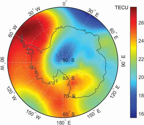
CODE is one of the Global Analysis Centers for IGS, and GIM is generated on a daily basis at CODE using data from about 200 GNSS sites of the IGS and other institutions. The GIM product is in the so-called IONosphere map EXchange format, and it provides worldwide TEC maps with 2-hour temporal resolution and 2.5° × 5° spatial resolution in latitude and longitude, respectively. The precision and reliability have long been proved by researchers (Hernández-Pajares et al. 2009), and it is widely used in a variety of applications as a $VTEC$ source. In this study, we interpolated GIM in both the time and space domains and obtained the $VTEC$ values for each observation epoch at each IPP in 2012. Figure 2 shows the $VTEC$ distribution 450 km above Antarctica at 0:00 UTC, 1 January 2012.

Figure 2. $VTEC$ distribution 450 km above Antarctica at 0:00 UTC, 1 January 2012. One TEC unit (TECU) = 10¹⁶ electrons/m²

International geomagnetic reference field: The twelfth generation

In this study, IGRF-12 was adopted to determine the magnetic field vector on the height of thin layer; that is, both the intensity and direction of ${\mathbf{B}}_{\mathbf{0}}$.

The IGRF is a series of mathematical models of the internal geomagnetic field and its annual rate of change. The latest IGRF-12 was released by the International Association of Geomagnetism and Aeronomy in December 2014 and provides a definitive geomagnetic reference field model for calculating the magnetic field in near-Earth space during epochs 1900 to 2020 (Thébault et al. 2015). On and above the surface of the Earth, the magnetic field $\mathbf{B}$ can be defined by the following equations:

(11) $\mathbf{B}=-\mathrm{\nabla }V$(11)

(12) $V(r,\theta ,\varphi ,t)=a\sum _{n=1}^N\sum _{m=0}^n{\left(\frac{a}{r}\right)}^{n+1}[g_n^m(t)cosm\varphi +h_n^m(t)sinm\varphi ]\times P_n^m(cos\theta )$(12)

with $V$ denoting the magnetic scalar potential. The symbols $r$, $\theta$, $\varphi$, and $t$ are used to determine the location and time in the geomagnetic coordinate system, where r denotes the radial distance from the center of the Earth, $a$ = 6,371.2 is the geomagnetic conventional mean reference spherical radius of the Earth, $g_n^m$ and $h_n^m$ are Gauss coefficients, and the function $P_n^m(cos\theta )$ is the Schmidt quasinormalized associated Legendre function with degree $n$ and order $m$.

Based on Equations (11)(11) $\mathbf{B}=-\mathrm{\nabla }V$(11) and (12(12) $V(r,\theta ,\varphi ,t)=a\sum _{n=1}^N\sum _{m=0}^n{\left(\frac{a}{r}\right)}^{n+1}[g_n^m(t)cosm\varphi +h_n^m(t)sinm\varphi ]\times P_n^m(cos\theta )$(12) ), the geocentric components of the geomagnetic field in the northward, eastward, and radially inward directions ($X$, $Y$, and $Z$) are given as

(13) $\begin{array}{ccc}X=\frac{1}{r}\frac{\mathrm{\partial }V}{\mathrm{\partial }\theta },& Y=-\frac{1}{rsin\theta }\frac{\mathrm{\partial }V}{\mathrm{\partial }\varphi },& Z=\frac{\mathrm{\partial }V}{\mathrm{\partial }r}\end{array}$(13)

As seen from the above, the magnetic field vector ${\mathbf{B}}_{\mathbf{0}}$ at IPP can thus always be calculated. Furthermore, the range vector from each GPS satellite to a local receiver at every epoch can be worked out by given ephemeris and coordinates files; thus, $cos(z^{\prime })$ and $cos{\theta }_B$ can also be calculated at the same time. The magnetic field distribution in Antarctica using IGRF-12 for 1 January 2012 and 450 km above the Earth is shown in Figure 3, calculated by the function “igrfmagm” in MATLAB Aerospace Toolbox (Blakely 1996; Lowes 2010).

Figure 3. Geomagnetic field intensity distribution in Antarctica on 1 January 2012 450 km above the surface of the Earth, calculated based on IGRF-12. (a) Total intensity and (b)–(d) the field intensity in the x, y, and z, directions, respectively. The unit of geomagnetic field intensity is nano Tesla

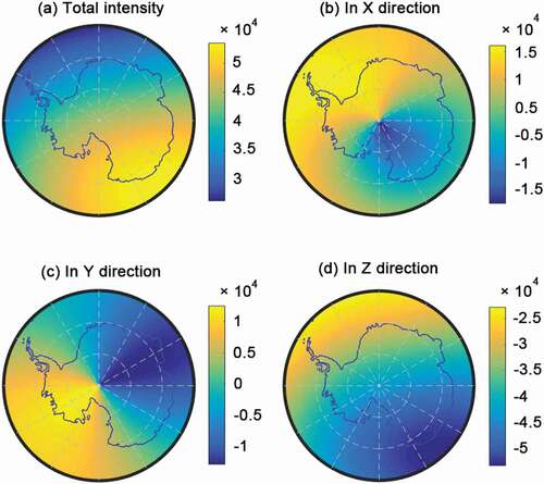
Research indicates that the former IGRF-10 and -11 models are quite compliant with the measured $\mathbf{B}$ field in the ionosphere 92.80 percent of the time (Matteo and Morton 2011). Because the IGRF-12 model is considered to be at least of the same accuracy, the latest model is of sufficient accuracy for use as input data in this study.

Distribution of Antarctic GPS stations

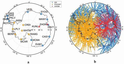
At present, there are tens of continuously operating GPS stations located in Antarctic continent (Figures 4 and 5a), and the most important observation networks are the IGS and POLENET networks. In addition, some scientific research stations have established their own GPS observing systems. IGS is the largest GPS observation network in the world, and its Antarctic observatories are mainly distributed along the coast; POLENET is primarily focused on collecting GPS and seismic data, and the observatories are distributed both along the coast and in some inland areas. In order to cover as much of the Antarctic continent as possible, we selected twelve stations from IGS, seven stations from POLENET, and two stations run by the Chinese Antarctic Center of Surveying and Mapping (CACSM), Wuhan University, as our input data, and the time span was the entire year 2012. The geographic distribution of the twenty-one stations is shown in Figure 5a, and Figure 5b depicts the IPP distribution of each station from 00:00 to 12:00 UTC to day 20120101, showing a good complementarity of different observed network data over the whole of Antarctica.

Figure 4. Antenna of continuously operating GPS system in Zhongshan Base, Larsemann Hills, East Antarctica. The GPS receiver type is LEICA GRX1200PRO, and the antenna type is LEIAT504

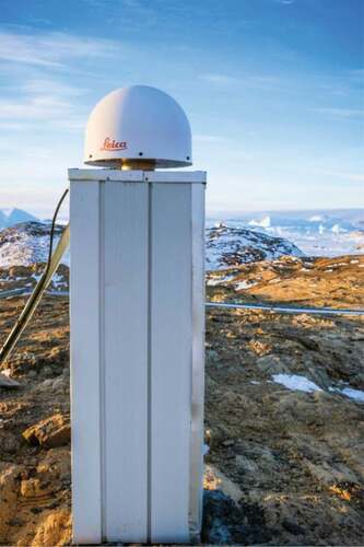
Figure 5. (a). Geographic distribution of the continuously operating GPS stations adopted in this study. Note that KUNL (Kunlun Base, China) is a summer station, only providing the data during January. (b). IPP distribution from 00:00 to 12:00 UTC on day 20120101

Estimation strategy

The residual GPS ranging error caused by the second-order ionospheric term was analyzed, as shown in Equation (10)(10) $I_{LC}=\left(-\frac{1}{2}\frac{1}{f_1(f_1^2-f_2^2)}+\frac{1}{2}\frac{1}{f_2(f_1^2-f_2^2)}\right)\times \frac{7527}{cos(z^{\prime })}\times c\times \left|{\mathbf{B}}_{\mathbf{0}}\right|\times cos{\theta }_B\times VTEC$(10) , and in the previous section all of the data sources are described in detail. In order to investigate the effect of the second-order ionospheric term on GPS positioning in Antarctica, the positioning error should correlate with the ranging error.

In addition to simulation, Geiger’s (1988) error estimation method proposes analytical or semianalytical solutions in many cases for estimating different disturbances in GPS measurements, and the method has been adopted in some research involving the second-order ionospheric term (Munekane 2005; Liu et al. 2010). Let us consider the coordinate system whose axes point toward the east, north, and vertical directions, respectively. The ranging error, $I_{LC}$, correlates with the positioning error as follows:

(14) $I_{LC}=C\cdot \mathbf{r}$(14)

(15) $\mathbf{C}=(e_1,e_2,e_3)$(15)

(16) $\mathbf{r}=(x,y,z{)}^T$(16)

where $\mathbf{C}$ is a design matrix and $\mathbf{r}$ is the GPS positioning error of a station. The components of $\mathbf{C}$ are given as

(17) $e_1=-sin\theta sin\lambda$(17)

(18) $e_2=-sin\theta cos\lambda$(18)

(19) $e_3=-cos\theta$(19)

with $\theta$ and $\lambda$ denoting the zenith and azimuth angles of the GPS satellite, respectively. The components x, y, and z in the vector $\mathbf{r}$ denote the positioning error in the east, north, and vertical directions, respectively. According to Equation (10)(10) $I_{LC}=\left(-\frac{1}{2}\frac{1}{f_1(f_1^2-f_2^2)}+\frac{1}{2}\frac{1}{f_2(f_1^2-f_2^2)}\right)\times \frac{7527}{cos(z^{\prime })}\times c\times \left|{\mathbf{B}}_{\mathbf{0}}\right|\times cos{\theta }_B\times VTEC$(10) and the equations above, the estimation equation is finally formed as

(20) $\left(-\frac{1}{2}\frac{1}{f_1(f_1^2-f_2^2)}+\frac{1}{2}\frac{1}{f_2(f_1^2-f_2^2)}\right)\times \frac{7527}{cos(z^{\prime })}\times c\times \left|{\mathbf{B}}_{\mathbf{0}}\right|\times cos{\theta }_B\times VTEC={\left(\begin{array}{c}-sin\theta sin\lambda \\ -sin\theta cos\lambda \\ -cos\theta \end{array}\right)}^T\cdot \left(\begin{array}{c}x\\ y\\ z\end{array}\right)$(20)

Considering that GPS is designed to receive signals from at least four different satellites anywhere on the Earth at any time, at least four (usually more than five and sometimes more than ten) values can be obtained for the left-hand side of Equation (20)(20) $\left(-\frac{1}{2}\frac{1}{f_1(f_1^2-f_2^2)}+\frac{1}{2}\frac{1}{f_2(f_1^2-f_2^2)}\right)\times \frac{7527}{cos(z^{\prime })}\times c\times \left|{\mathbf{B}}_{\mathbf{0}}\right|\times cos{\theta }_B\times VTEC={\left(\begin{array}{c}-sin\theta sin\lambda \\ -sin\theta cos\lambda \\ -cos\theta \end{array}\right)}^T\cdot \left(\begin{array}{c}x\\ y\\ z\end{array}\right)$(20) at every epoch. On the right-hand side, the number of unknown parameters is only three, namely, $x$, $y$, and $z$. Hence, the positioning errors can be estimated by least squares. Because the sampling rate of network IGS, POLENET, and CACSM stations is always 1/30 Hz or higher, within a single day, more than 2,000 sets of estimates can be obtained. In this study, we solved the estimates on the twenty-one stations for the whole year for 2012 and then analyzed them as time series. Figure 6 shows a flowchart of the data processing.

Figure 6. Flowchart of the data processing. TEQC (Translation, Editing, and Quality Check; Estey and Meertens 1999) and GPSTk (GPS Toolkit; Harris and Mach 2007) were used in the GPS preprocessing, and least squares estimation was undertaken in MATLAB software

Results and discussion

We estimate the positioning error caused by the second-order ionospheric term for each station at a sampling interval of 30 seconds over the course of the year 2012. Time series of the positioning error are shown in Figure 7 and the mean values are shown in Table 1. The mean values are calculated in two ways, in which the annual mean value is used to describe the size of the positioning error for the entire year 2012, and the mean values in January and July are used respectively to represent the characteristics of the positioning error in the Antarctic summer and winter.

Table 1. Mean values of GPS positioning errors in x, y, and z directions for each station derived by the second-order ionospheric term during the whole year for 2012 (mm)

Station name	Mean value yearly			Mean value in January			Mean value in July
	x	y	z	x	y	z	x	y	z
BERP	0.145	−1.316	1.583	0.280	−2.132	2.564	0.016	−0.399	0.474
CAS1	0.146	−1.589	1.839	0.195	−2.377	2.675	0.081	−0.622	0.770
CRDI	0.275	−0.279	1.292	0.504	−0.476	2.289	0.089	−0.076	0.318
DAV1	−0.141	−1.570	1.537	−0.222	−2.304	2.309	−0.051	−0.586	0.587
DUM1	−0.061	−1.203	1.798	−0.125	−1.783	2.606	−0.009	−0.491	0.786
JNSN	0.590	−0.802	1.451	0.811	−1.287	2.285	0.191	−0.215	0.361
KUNL	—	—	—	0.198	−1.286	3.023	—	—	—
LPLY	0.383	−1.067	1.244	0.717	−1.996	2.418	0.149	−0.338	0.417
MAW1	−0.419	−1.375	1.403	−0.573	−1.913	2.048	−0.146	−0.462	0.490
MCAR	−0.298	−0.907	1.590	−0.454	−1.304	2.465	−0.136	−0.349	0.550
MCM4	−0.230	−0.300	1.576	−0.187	0.221	2.188	−0.120	−0.145	0.617
OHI2	0.601	−0.618	1.067	0.973	−0.930	1.737	0.183	−0.213	0.367
OHI3	0.766	−0.595	1.119	1.246	−1.037	1.865	0.280	−0.154	0.384
PALM	0.759	−0.736	1.150	1.304	−1.265	1.977	0.259	−0.158	0.372
PALV	0.758	−0.718	1.158	1.299	−1.229	1.999	0.255	−0.158	0.375
RAMG	−0.091	−0.056	1.443	−0.006	−0.232	2.340	−0.055	0.037	0.487
ROTH	0.753	−0.796	1.225	1.303	−1.353	2.127	0.255	−0.223	0.370
SYOG	−0.412	−0.894	1.184	−0.496	−1.561	1.785	−0.144	−0.205	0.376
VESL	−0.083	−0.200	1.069	0.021	−0.422	1.778	−0.028	−0.012	0.327
WHTM	0.199	−0.846	1.549	0.423	−1.485	2.615	0.033	−0.198	0.431
ZHON	−0.138	−1.451	1.529	−0.234	−2.180	2.291	−0.048	−0.531	0.567
Total	0.175	−0.866	1.390	0.332	−1.349	2.256	0.053	−0.275	0.471

Note. Refer to Figure 5 for GPS station positions.

Figure 7. Time series of positioning errors derived by the second-order ionospheric term for twenty-one Antarctic GPS stations in 2012. Components x, y, and z represent the positioning errors in the east, north, and vertical directions, respectively

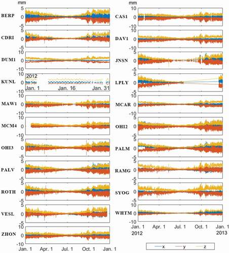
It can be seen from Figure 7 that the effect of the second-order ionospheric term on GPS positioning over these stations is on the submillimeter to millimeter level. The effect in each direction is generally different, and the effect in the x direction is obviously less than that in the y or z direction in size. In addition, the values of y are always negative, whereas the values of z are always positive. In addition, the positioning error on each station is rather small in Antarctic winter, whereas it becomes several times larger in Antarctic summer, and the effects on all of the stations seem to share certain degrees of synchronization at the timescale.

As seen from Table 1, the yearly average positioning error derived from the second-order ionospheric term in the x, y, and z directions is 0.175, −0.866, and 1.390 mm, respectively. Moreover, the effect in January (Antarctic summer) is much higher than it is in July (Antarctic winter) by 5.33 times on average in each direction. According to the mean values of positioning error, Figure 8 was drawn to show the motion derived by the second-order term for each station.

Figure 8. Yearly motion for each GPS station derived by the second-order ionospheric term. The arrows represent the size and direction of horizontal movement, and the depth of the color represents the size of the upward movement

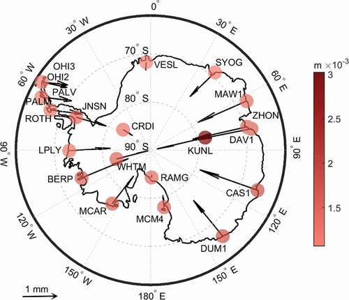
Figure 8 shows that all GPS stations have a tendency to drift toward the south in the horizontal direction and upward in the vertical direction. In other words, if only the first-order ionospheric term were considered for these stations, as the commonly used ionospheric-free combination in Equation (9)(9) $\begin{array}{c}LC=\frac{f_1^2}{f_1^2-f_2^2}{L}_1-\frac{f_2^2}{f_1^2-f_2^2}{L}_2(9)\\ \\ !=\rho +I_{LC}\end{array}$(9) , the residual errors of the second-order ionospheric term would derive a tendency of moving toward the South Pole horizontally and upward vertically.

On the other hand, according to Equation (20)(20) $\left(-\frac{1}{2}\frac{1}{f_1(f_1^2-f_2^2)}+\frac{1}{2}\frac{1}{f_2(f_1^2-f_2^2)}\right)\times \frac{7527}{cos(z^{\prime })}\times c\times \left|{\mathbf{B}}_{\mathbf{0}}\right|\times cos{\theta }_B\times VTEC={\left(\begin{array}{c}-sin\theta sin\lambda \\ -sin\theta cos\lambda \\ -cos\theta \end{array}\right)}^T\cdot \left(\begin{array}{c}x\\ y\\ z\end{array}\right)$(20) , the positioning error is positively correlated with the $VTEC$ value. Because local $VTEC$ is closely related to solar activity, there is a strong seasonal variation. After observing the seasonal variations of the time series for each station as well in Figure 7, it is reasonable to make an assumption that the positioning error and local $VTEC$may be positively correlated and synchronized in the time domain. Based on GIM, Figure 9 shows the averaged $VTEC$ values above all twenty-one stations in the whole year 2012.

Figure 9. Average $VTEC$ values over all twenty-one stations for the year 2012. The time interval was set to every 2 hours

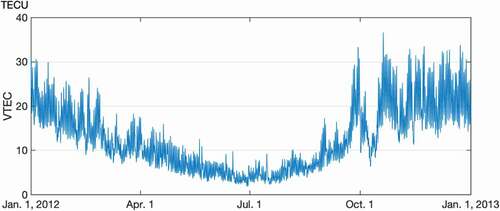
It is clearly inferred from Figure 9 that the trend of $VTEC$ shows a positive correlation with the positioning errors in Figure 7 in the time domain. In Antarctic summer—that is, the beginning and end of the year—influenced by polar day phenomenon, $VTEC$ remains at a relatively higher level, resulting in the positioning error in each direction becoming larger; in contrast, in Antarctic winter—that is, the middle of the year—influenced by polar night phenomenon, $VTEC$ plummets, and the positioning error in each direction decreases accordingly. Moreover, in Figure 9, the $VTEC$ values were reduced abnormally in October, and this anomaly is confirmed in Figure 7. 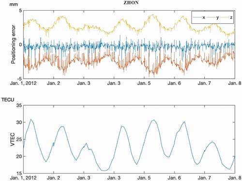In order to better demonstrate the synchronization of $VTEC$ and the positioning error derived by the second-order ionospheric term, we narrowed the timescale to the first week of 2012, taking Zhongshan station (ZHON) as an example, and drew Figure 10.

Figure 10 shows the correlation and synchronization of the positioning error and the $VTEC$ in a more obvious way. Even when the $VTEC$ changes in a diurnal sense, there would be reflection on positioning error accordingly.

Figure 10. Relation of $VTEC$ and the positioning error for the first week of 2012. The top panel shows the effect of the second-order ionospheric term on GPS positioning in the x, y, and z directions at ZHON station. The bottom panel shows the average $VTEC$ values over the twenty-one stations

Summary and conclusions

This study aimed to investigate the effect of the second-ionospheric term on GPS positioning in Antarctica. First, the commonly used so-called ionospheric-free combination was given, by which the first-order ionospheric term is totally eliminated. Second, the residual ranging error derived by the second-order ionospheric term was introduced and the positioning error in each direction was derived. GIM and IGRF-12 were adopted to provide the values of the vertical total electron content and the geomagnetic field of the Earth. GPS data from twenty-one continuously operating stations in Antarctica from the IGS, POLENET, and CACSM networks were used as our data source. Based on the principles and data, the positioning errors in each direction were estimated by a least-squares method for the whole year for 2012.

Results show that the effect of the second-order ionospheric term on GPS positioning in 2012 is on the submillimeter to millimeter level, and the yearly average positioning error for the twenty-one stations in east, north, and vertical directions is 0.175, −0.866, and 1.390 mm, respectively. The effect in the east direction is less than that in the north and vertical directions in size, and all of the stations show the southward and upward movement derived from the effect. Moreover, the effect in Antarctic summer is 5.33 times higher than it is in winter on average in each direction. On the other hand, according to the positioning error variation in the time domain, we analyzed the relationship between the positioning error and $VTEC$ and found that the positioning error and local $VTEC$ are positively and highly correlated and synchronized. Therefore, when conducting high-precision research or applications related to Antarctica, the effect of the second-order ionospheric term on positioning should not be ignored, especially when TEC is high.

Today, research related to Antarctica is increasingly valued by research communities around the world, and GPS as a major or auxiliary method is widely used to obtain high-precision spatial position, displacement, or velocity information, especially in the case of plate movement, ice flow velocity, postglacial rebound, etc. This article may provide researchers with a new perspective on future data processing.

Moreover, this article only uses the most popular GPS (U.S.) system here as an example; however, the current trend is that increasing numbers of observing systems are beginning to integrate GLONASS (Russia), BDS (China), and GALILEO (EU) systems for greater precision and stability, and many IGS tracking stations located in the Antarctic have already integrated multimode GNSS observations. The influential mechanism of the ionosphere on them is similar to that of GPS. However, because the signal frequency and other characteristics are not the same, the magnitude of the impact requires further study, which is one of our future research directions. On the other hand, we look forward to extend the experimental time span to a much longer period, such as an entire solar cycle, and this will better reflect the relationship between solar activity and GNSS positioning error.

Acknowledgments

We thank IGS for managing and providing free GPS data from hundreds of continuous stations to researchers worldwide. POLENET data are based on services provided by the GAGE Facility, operated by UNAVCO, Inc., with support from the National Science Foundation and the National Aeronautics and Space Administration under NSF Cooperative Agreement EAR-1724794. We thank the International Association of Geomagnetism and Aeronomy for releasing the IGRF-12 model.

Disclosure Statement

No potential conflict of interest was reported by the authors.

Additional information

Funding

This study was supported by the National Natural Science Foundation of China (Nos. 41730102, 41941005, 41776195, and 41776186).

References

- Argus, D. F., W. R. Peltier, R. Drummond, and A. W. Moore. 2014. The Antarctica component of postglacial rebound model ICE-6G_C (VM5a) based on GPS positioning, exposure age dating of ice thicknesses, and relative sea level histories. Geophysical Journal International 198 (1):537–63. doi:https://doi.org/10.1093/gji/ggu140.
- Bassiri, S., and G. Hajj. 1993. Higher-order ionospheric effects on the GPS observables and means of modeling them. Advances in the Astronautical Sciences 82 (2):1071–86.
- Blakely, R. J. 1996. Potential theory in gravity and magnetic applications. Cambridge, UK: Cambridge University Press.
- Capra, A., F. Mancini, and M. Negusini. 2007. GPS as a geodetic tool for geodynamics in northern Victoria Land, Antarctica. Antarctic Science 19 (1):107–14. doi:https://doi.org/10.1017/S0954102007000156.
- Crawford, F. S. 1968. Waves, Vol. 3. New York: Tata McGraw-Hill Education.
- Dietrich, R., A. Rülke, J. Ihde, K. Lindner, H. Miller, W. Niemeier, H.-W. Schenke, and G. Seeber. 2004. Plate kinematics and deformation status of the Antarctic Peninsula based on GPS. Global and Planetary Change 42 (1–4):313–21. doi:https://doi.org/10.1016/j.gloplacha.2003.12.003.
- Donnellan, A., and B. P. Luyendyk. 2004. GPS evidence for a coherent Antarctic plate and for postglacial rebound in Marie Byrd Land. Global and Planetary Change 42 (1–4):305–11. doi:https://doi.org/10.1016/j.gloplacha.2004.02.006.
- Dow, J. M., R. E. Neilan, and C. Rizos. 2009. The international GNSS service in a changing landscape of global navigation satellite systems. Journal of Geodesy 83 (3–4):191–98. doi:https://doi.org/10.1007/s00190-008-0300-3.
- Estey, L. H., and C. M. Meertens. 1999. TEQC: The multi-purpose toolkit for GPS/GLONASS data. GPS Solutions 3 (1):42–49. doi:https://doi.org/10.1007/PL00012778.
- Frezzotti, M., A. Capra, and L. Vittuari. 1998. Comparison between glacier ice velocities inferred from GPS and sequential satellite images. Annals of Glaciology 27:54–60. doi:https://doi.org/10.3189/1998AoG27-1-54-60.
- Fritsche, M., R. Dietrich, C. Knöfel, A. Rülke, S. Vey, M. Rothacher, and P. Steigenberger. 2005. Impact of higher‐order ionospheric terms on GPS estimates. Geophysical Research Letters 32 (23). doi:https://doi.org/10.1029/2005GL024342.
- Geiger, A. 1988. Simulating disturbances in GPS by continuous satellite distribution. Journal of Surveying Engineering 114 (4):182–94. doi:https://doi.org/10.1061/(ASCE)0733-9453(1988)114:4(182).
- Harris, R. B., and R. G. Mach. 2007. The GPSTk: An open source GPS toolkit. GPS Solutions 11 (2):145–50. doi:https://doi.org/10.1007/s10291-006-0043-7.
- Hernández-Pajares, M., J. M. Juan, J. Sanz, À. Aragón-Àngel, A. García-Rigo, D. Salazar, and M. Escudero. 2011. The ionosphere: Effects, GPS modeling and the benefits for space geodetic techniques. Journal of Geodesy 85 (12):887–907. doi:https://doi.org/10.1007/s00190-011-0508-5.
- Hernández-Pajares, M., J. M. Juan, J. Sanz, R. Orus, A. Garcia-Rigo, J. Feltens, A. Komjathy, S. C. Schaer, and A. Krankowski. 2009. The IGS VTEC maps: A reliable source of ionospheric information since 1998. Journal of Geodesy 83 (3–4):263–75. doi:https://doi.org/10.1007/s00190-008-0266-1.
- Kedar, S., G. A. Hajj, B. D. Wilson, and M. B. Heflin. 2003. The effect of the second order GPS ionospheric correction on receiver positions. Geophysical Research Letters 30 (16). doi:https://doi.org/10.1029/2003GL017639.
- Klobuchar, J. A. 1996. Ionospheric effects on GPS.Global Positioning System: Theory and Applications, Vol. I, ed. B. W. Parkinson and J. J. Spilker, 485–515. Reston, VA: American Institute of Aeronautics & Astronautics.
- Krankowski, A., I. I. Shagimuratov, L. W. Baran, and I. I. Ephishov. 2005. Study of TEC fluctuations in Antarctic ionosphere during storm using GPS observations. Acta Geophysica Polonica 53 (2):205–18.
- Liu, X., Y. Yuan, X. Huo, Z. Li, and W. Li. 2010. Model analysis method (MAM) on the effect of the second-order ionospheric delay on GPS positioning solution. Chinese Science Bulletin 55 (15):1529–34. doi:https://doi.org/10.1007/s11434-010-3070-2.
- Lowes, F. J. 2010. The international geomagnetic reference field: A “health” warning. http://www. ngdc. noaa. gov/IAGA/vmod.
- Mannucci, A. J., B. D. Wilson, D. N. Yuan, C. H. Ho, U. J. Lindqwister, and T. F. Runge. 1998. A global mapping technique for GPS-derived ionospheric total electron content measurements. Radio Science 33 (3):565–82. doi:https://doi.org/10.1029/97RS02707.
- Manson, R., R. Coleman, P. Morgan, and M. King. 2000. Ice velocities of the Lambert Glacier from static GPS observations. Earth, Planets and Space 52 (11):1031–36. doi:https://doi.org/10.1186/BF03352326.
- Matteo, N. A., and Y. T. Morton. 2011. Ionosphere geomagnetic field: Comparison of IGRF model prediction and satellite measurements 1991–2010. Radio Science 46 (4):1–10. doi:https://doi.org/10.1029/2010RS004529.
- Morton, Y. T., F. van Graas, Q. Zhou, and J. Herdtner. 2009. Assessment of the higher order ionosphere error on position solutions. Navigation 56 (3):185–93. doi:https://doi.org/10.1002/navi.2009.56.issue-3.
- Munekane, H. 2005. A semi-analytical estimation of the effect of second-order ionospheric correction on the GPS positioning. Geophysical Journal International 163 (1):10–17. doi:https://doi.org/10.1111/gji.2005.163.issue-1.
- Schaer, S.; Société helvétique des sciences naturelles. Commission géodésique. 1999. Mapping and predicting the Earth’s ionosphere using the global positioning system, Vol. 59. Bern: Institut für Geodäsie und Photogrammetrie, Eidg. Technische Hochschule Zürich.
- Suparta, W., Z. A. A. Rashid, M. A. M. Ali, B. Yatim, and G. J. Fraser. 2008. Observations of Antarctic precipitable water vapor and its response to the solar activity based on GPS sensing. Journal of Atmospheric and Solar-Terrestrial Physics 70 (11–12):1419–47. doi:https://doi.org/10.1016/j.jastp.2008.04.006.
- Thébault, E., C. C. Finlay, C. D. Beggan, P. Alken, J. Aubert, O. Barrois, and E. Canet. 2015. International geomagnetic reference field: The 12th generation. Earth, Planets and Space 67 (1):79. doi:https://doi.org/10.1186/s40623-015-0228-9.
- Tiwari, S., A. Jain, S. Sarkar, S. Jain, and A. K. Gwal. 2012. Ionospheric irregularities at Antarctic using GPS measurements. Journal of Earth System Science 121 (2):345–53. doi:https://doi.org/10.1007/s12040-012-0168-8.