4-Nonylphenol in Sierra Nevada glaciers, California, USA

ABSTRACT

Persistent organic pollutants are stored in environmental reservoirs globally. Tracking the mass and movement of these pollutants is critical for assessing environmental health for human and wildlife populations. Recently, glaciers have been identified as secondary reservoirs for persistent organic pollutants. Downstream lakes and rivers have increased risk of exposure with climate change and loss of glacier mass. Two glaciers, Palisade and Middle Palisade Glaciers, in the Sierra Nevada Mountains, California, United States, were modeled for total mass of the persistent organic pollutant, 4-nonylphenol (4NP). The model used LiDAR measurements of surface snow and geographic information systems (GIS) to extrapolate vertical and horizontal 4NP gradients. Concentrations of 4NP in surface snow were sampled in locations based on a range of topographical shielding indices and analyzed via gas chromatography–mass spectrometry. The Middle Palisade Glacier, the smaller and more shielded glacier, had a total mass of 1,677 ± 560 kg 4NP/km². The Palisade Glacier, which is larger and more exposed to atmospheric deposition, held an estimated 3,456 ± 843 kg 4NP/km². Meltwater concentrations for the Middle Palisade and Palisade Glaciers were 1.3 ± 0.05 μg/L and 6.1 ± 1.3 μg/L, respectively. These values demonstrate that both glaciers store a significant amount of 4NP and will act as secondary sources of 4NP for downstream water bodies.

KEYWORDS:

• Persistent organic pollutants
• glacier reservoirs
• 4-nonylphenol
• Sierra Nevada mountains

Introduction

Persistent organic pollutants (POPs) are globally distributed through atmospheric transport. Aerosols and dust-borne contaminants are capable of long-range transport over oceans and continents and along a latitudinal gradient (Shao et al. 2011). Traces of polychlorinated biphenyls (PCBs) have been found in the Antarctic Peninsula, hundreds of kilometers from the source (Khairy et al. 2016). Once deposition has occurred in a region, depending on the terrain, POPs can be stored for long periods of time (Kirchgeorg et al. 2016). Glaciers are known to accumulate atmospherically derived contaminants and have provided records of the deposition of POPs over time (Gregor et al. 1995; Donald et al. 1999). These compounds are then re-released into meltwater or spring runoff. In some regions with a history of industrial legacy pollutants, glaciers are considered a secondary pollutant source for POPs in downstream lakes and rivers (Bogdal et al. 2010).

4-Nonylphenol (4NP) is a persistent organic pollutant that mimics the female sex hormone 17-β-estradiol, causing it to behave as an endocrine disruptor, with significant consequences on reproductive health in humans and wildlife (Vazquez-Duhalt et al. 2005). 4NP is generated from the breakdown of the surfactant nonylphenol polyethoxylate (NPE) and through direct manufacture. It is estimated that between 45 and 230 million kilograms of NPE are produced globally every year (U.S. Environmental Protection Agency [U.S. EPA] 2010). Due to increasing regulations, the use of NPEs in the United States has not increased in recent years (Ying, Williams, and Kookana 2002); however, global production of NPE has increased (Bergé et al. 2012). The U.S. EPA has set water quality criteria for 4NP at 6.6 μg/L for acute exposure and 1.7 μg/L for chronic exposure (U.S. EPA 2005). As of 2018, 4NP and its parent compound have been added to the list of substances that require a Toxic Release Inventory (U.S. EPA 2010). Other countries have set more stringent maximum contamination limits on 4NP concentrations. For example, Environment Canada has limits that are more conservative at 0.7 μg/L for chronic exposure (Canadian Council of Ministers of the Environment 2002).

Compounds with low water solubility like 4NP are more likely to undergo long-range transport due to their affinity for the organic moiety of dust particulates (Beyer et al. 2000). The organic carbon partition coefficient (log K_OC) describes the tendency of a compound to absorb to the organic carbon fraction of particulates. This can be determined through a linear free energy relationship with the octanol–water partition coefficient

(1) $Log{K}_{OC}=a\left(log{K}_{OW}\right)+b,$(1)

where a and b are coefficients dictated by the nature of the compound (Schwarzenbach and Gschwend 2016). The log K_OC for 4NP, based on a log K_OW of 4.48, has been calculated to be 4.03 using the coefficients 0.79 and 0.49 for a and b, respectively, for alkylphenols (Schwarzenbach and Gschwend 2016). This shows susceptibility for 4NP to bind and travel attached to particulate matter and agrees with the experimental values determined by Burgess et al. (2005). 4NP also potentially travels as an aerosol due to its relatively high octanol–air partitioning ability (log K_OA), which is on the order of 7.9 (Lyons, Van de Bittner, and Morgan-Jones 2014). Wania and Dugani (2003) suggested that a log K_OA between 6.5 and 10 allows for long-range aerosol transport of persistent organic pollutants.

Because of 4NP’s tendency to partition to organic material, the highest environmental concentrations of 4NP can be found in soil and sediment. In a Minnesota study, river water and sediment were tested downstream of a wastewater treatment plant (Writer et al. 2012). Water concentrations were 0.620 ± 0.390 μg/L and sediment was found to have 140 μg 4NP/kg. Wastewater treatment plant effluent in particular can have especially high concentrations of 4NP, averaging 2.84 μg/L near Southern California wastewater treatment outflow (Bulloch et al. 2015). Volatilization of 4NP can cause some atmospheric concentrations to be as high as 2.2 to 70 ng/m³ (Dachs, Van Ry, and Eisenreich 1999). Once airborne, 4NP will partition to dust, rain, or snow (Lei and Wania 2004). A study of 4NP concentrations in rain and snow showed an average concentration of 0.253 μg/L in rain and 0.242 μg/L in snow meltwater (Fries and Püttmann 2004).

Snow in flight can scavenge particles and aerosol during formation (Wania et al. 1998). Because of this ability, snow is capable of adsorbing aerosol and particulate-bound 4NP. As a result, in seasonal snowpack, significant concentrations of 4NP are expected. Lyons, Van de Bittner, and Morgan-Jones (2014) found that seasonal snow concentrations were 10 to 100 times higher than surface water concentrations. As seasonal snow melts, meltwater is filtered through soils and eventually joins with surface water. Burgess et al. (2005) suggested that there is little movement of 4NP once it reaches the soil due to its high K_OC value. However, in the case of glaciers or permanent snowfields, meltwater does not encounter soil until it reaches the subglacial till. Glaciers effectively become a reservoir for POPs that could potentially last for decades. For example, legacy pollutants such as PCBs that have not been in use for decades are being released from Swiss glaciers (Bogdal et al. 2010; Kirchgeorg et al. 2016).

Climate change can drive change in the chemistry of glacier meltwater. Increased melt rates mean that concentrations of POPs in meltwater increase (Bogdal et al. 2010). Current use pesticides have been found in the meltwater of the Lys and Forni Glaciers in the Italian Alps (Ferrario, Finizio, and Villa 2017). Concentrations ranged from 1.0 to 2.5 μg/L. These glaciers are located downwind of agricultural areas, similar to the Sierra Nevada glaciers. POPs, including organochloride pesticides, were found in glacier meltwater from more remote glaciers in the Canadian Rockies, with concentrations ranging from 0.1 to 0.2 μg/L, an order of magnitude less than that in glacier meltwater near agricultural regions (Blais et al. 2001). Organochloride pesticides have been detected in Himalayan glacier snow samples, although meltwater from glaciers in this region primarily carries legacy pollutants such as polycyclic aromatic hydrocarbons and PCBs (Kang et al. 2009; Sharma et al. 2015). Therefore, it can be expected that climate-driven changes in chemistry of discharged meltwater may be having global effects on adjacent headwater ecosystems.

The Sierra Nevada mountains create a physical barrier between western California’s Central Valley and the Great Basin Range to the east. The Central Valley is one of the most productive agricultural regions in the United States, with heavy pesticide use and periodic droughts (Sunding et al. 1997). Particle-bound and aerosolized 4NP have been shown to undergo long-range transport over the Sierra Nevada and deposit on the east side (Lyons, Van de Bittner, and Morgan-Jones 2014). The prevailing wind direction is consistently from the west to the east, making this a convenient system for modeling. The Sierra Nevada Range receives the majority of its precipitation as snow and is home to several low-latitude glaciers (Molotch and Meromy 2014). Because of the economic importance of the seasonal snowpack as a water source for the Los Angeles basin, snow volumes are carefully monitored in this region.

Recently, LiDAR has become the tool of choice for snow volume measurements through the Jet Propulsion Laboratory’s Airborne Snow Observatory. LiDAR systems are composed of active sensors that transmit light pulses to produce highly accurate measurements of the Earth’s surface. LiDAR systems integrate three technologies: laser ranging for distance measurement, Global Positioning System (GPS) to determine the sensor’s geographic position and height, and an inertial measurement unit to record the precise orientation of the sensor on the aircraft (Aronoff 2004). Recent studies have proposed LiDAR as a safe, cost-effective, and efficient method of mapping snow depth (Deems et al. 2013).

The goal of this study is to estimate the total mass of 4NP currently stored in the Palisades (37.0992° N; 118.5097° W) and Middle Palisade Glaciers (37.07149° N; 118.4575° W) of the Sierra Nevada mountains, California. Glaciers in this region of the Sierra Nevada are young, appearing in the Little Ice Age about 700 years ago (Matthes 1939). These high-elevation glaciers (3,960 m) have surface areas of 1.3 and 0.34 km², respectively. Using LiDAR volume measurements in combination with geographical information systems (GIS), seasonal snow and glacier volumes were accurately calculated and combined with field measurements. This model was then used to determine the mass of 4NP in the Middle Palisade and Palisade Glaciers.

Methods

LiDAR snow measurements

The National Aeronautics and Space Administration’s Airborne Snow Observatory collects data during two periods, snow-covered and snow-free, to analyze seasonal snow changes. To calculate snow depth, two LiDAR data collections representing snow-free and snow-covered dates are required (Deems et al. 2013). The generation of digital elevation models (DEMs) from the LiDAR capture of surfaces allows for the examination of snow depth changes. Subtracting the difference between the two data sets provides snow depth for the area of interest. Snow volume was determined based on snow depth. Snow coverage from the Airborne Snow Observatory was recovered in LiDAR data exchange (LAS) files, and DEMs were taken from LiDAR raster files. Both data sets included point cloud data that covered the research study area. The first set of point cloud data was collected on 30 August 2014 and served as the snow-off layer. A second set of point cloud data collected on 28 April 2018 served as snow-on. The Create LAS Dataset tool in ArcGIS Pro (Version 2.5, ESRI) was used to create two LAS data sets representing snow-on and snow-off. Specifying WGS 1984 UTM Zone 11 N as the horizontal coordinate system and WGS 1984 as the vertical coordinate system verified that there were point cloud data in the glaciers of interest. A polygon feature class was created of the target area, and the point cloud data of the glacier area of both data sets were isolated using the Extract LAS tool.

The workflow for processing the data is shown in Figure 1. The snow-covered surface served as the digital surface model (DSM), and the snow-free surface was represented as the digital terrain model (DTM). The digital height model (DHM) is the result of the difference between the surface model and terrain model (Equation (2)(2) $DHM=DSM-DTM.$(2) )(2) $DHM=DSM-DTM.$(2) .

(2) $DHM=DSM-DTM.$(2)

Figure 1. Outline of the workflow from LiDAR data to snow volume done in ArcGIS Pro

The DHM was generated using the Minus Geoprocessing tool to subtract cell values of the two corresponding rasters. This stores the snow elevation difference of the two snow coverage periods as the height (z) value of each cell in the DHM. The DHM was then clipped to the glacial snow area using the Extract by Mask tool so that cells contained in the area were included in the raster. After the DHM was generated, any negative values were set as null and removed from future calculations. The raster’s values were then multiplied by the raster’s spatial resolution. This resulting raster contained the components of a cuboid in each cell necessary for volume measurements: the height (z), width (x), and length (y) of the cell. This transformed the DHM into a raster that contained a snow volume value for each cell. Total seasonal snow volume was quantitatively described by using the Zonal Statistics as Table tool to find the sum of all cell values. This final additional step reported an estimation of the total accumulation of snow between two time periods. Data are shown in Table 1. Error bars represent the measurement uncertainty.

Table 1. Values derived from snow-on/snow-off differences in LiDAR measured snow volume for the year 2014 (snow-off) and 2018 (snow-on)

LiDAR study area	Surface area^a (m^2)	LiDAR seasonal snow depth (m) (2018)	Seasonal snow volume (compacted) (m^3)
Palisade Glacier	1,293,990 ± 6,567	1.8 ± 0.0083	2,328,530 ± 23,285
Middle Palisade Glacier	342,300 ± 990	2.75 ± 0.0155	939,970 ± 9,400

Note. ^aSurface area measured with ArcGIS Pro polygon tool. All values shown with first standard deviation for measured area values.

Topographic shielding index

In some cases, measured concentrations were used for 4NP mass calculations, but not all regions of a glacier are accessible for direct measurement. The horizontal distribution of an airborne pollutant is not homogeneous. Distribution is dependent on the topography of the region, the source of the contaminant, and the prevailing wind direction (Lyons, Van de Bittner, and Morgan-Jones 2014; Lyons and Benvenuti 2016). These parameters were used to determine the topographical shielding coefficient ($\tau$). Shielding describes the interference of physical topography with atmospheric deposition of particulate matter and associated pollutants.

The topographic shielding index denoted as (τ), an indicator of the shielding effect of a ridgeline or physical barrier, is calculated as

(3) $\tau =\frac{S\ast H}{D},$(3)

where S is the slope of the ridge, H is the height of the ridge from the sample site, and D is the horizontal distance from the same sample site.

To automate and simplify the topographic shielding calculation workflow, a model was constructed in ModelBuilder as a geoprocessing tool in a toolbox. The model incorporates wind direction, distance, elevation, and slope values in the calculation. The custom tool prompts the user for parameter inputs for model execution. The inputs include a point feature class containing elevation, slope, and wind direction fields; a ridgeline segment with elevation and slope; and a polygon used to clip geodetic lines to measure distances to the ridge. The model was performed with a 90-m input point grid that contained slope and elevation fields that were spatially joined from a U.S. Geological Survey DEM.

The model consisted of a series of steps. There are three components to prepare the shielding calculation visualized in Figure 2. A copy of the input feature points was made and given X and Y coordinates in UTM at a resolution of 90 × 90 m. A minimum bounding geometry was created to encircle all of the points in the input feature class. The diameter of the minimum bounding geometry was calculated and reported as the “extend distance.” Using the wind direction field as a parameter, a new feature class containing the shortest line connecting two points was generated using the Bearing Distance to Line tool. These line features, known as geodetic lines, were based on the values reported in the X and Y coordinates, distance, and the newly introduced bearing or wind direction field.

Figure 2. The model workflow for the topographical shielding index is graphically represented in three steps

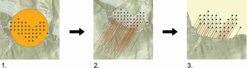
Finally, these geodetic lines were clipped to the ridgeline polygon, provided as an input parameter. A ridge distance field was added to the line feature class and populated by the geodetic length of each line feature calculated using the Calculate Geometry Attribute tool. The input parameter ridgeline line feature class containing elevation and slope for each feature segment was spatially joined to the geodetic line features. Fields were joined so that the result was a point feature class containing the variables needed to calculate topographic shielding values. Lastly, the shielding value was calculated by dividing the product of slope and the ridge elevation difference by the horizontal distance to the ridge. The topographic shielding value is reported without units as a scalar number for each input point. Wind direction for the region was taken from the National Renewable Energy Labs data set (National Renewable Energy Labs 2018). It should be noted that wind direction is nearly uniformly from west to east in the Sierra Nevada. The Pacific Ocean is a significant heat sink to the west, and orographic uplift creates almost continuous easterly winds. Because of these geographic factors, modeling this region can make use of the consistent weather patterns.

Sample site selection and sample collection

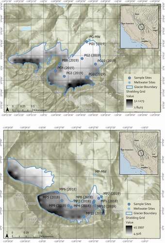
Sample sites were selected to be representative of the range of conditions on each glacier (Figures 3a and Figure 3b). Some areas were inaccessible due to hazardous conditions. Topographical shielding values were used to extrapolate concentrations that could not be accessed. A land ridge separates the Middle Palisade Glacier into two sections. Only the southern section of the Middle Palisades Glacier is included in this study. From this point on, reference to the Middle Palisade Glacier indicates the southern section of the Middle Palisades. Samples were acquired in June and August 2018 and June 2019.

Figure 3. (a) Sampling locations on the Palisade Glacier shown here with shielding index value gradient overlaid (37.1009° N, 118.5116° W). GPS points refer to glacier center mean. (b) Sampling locations on the Middle Palisade Glacier for 2018 and 2019 shown here with shielding index value gradient (37.0703° N, 118.4620° W). GPS points refer to glacier center mean for the southern section of the Middle Palisade Glacier. The northern section of the Middle Palisade Glacier (37.0753° N, 118.4687° W) was not sampled due to inaccessibility

Snow core sampling methods were followed according to U.S. Department of Agriculture field sampling guidelines (U.S. Department of Agriculture 1984). Snow core samples were performed in triplicate for each location to an average depth of 1.0 ± 0.2 m. Snow density was determined in situ by weighing the empty snow core, taking the samples, and then weighing the snow core with the snow. Snow mass was divided by the sample volume to find density. In the field, samples were stored in 2 L hexane-rinsed Mylar (Impak Corporation) bags. The reagent-grade hexane used in the field was obtained from Sigma Aldrich. Field blanks were created using 500 mL of deionized water transferred to a sampling bag while in the field. Snow water volume per snow core averaged 0.485 ± 0.25 L. After transport, melted samples were transferred to 1 L hexane-rinsed amber jars and acid-shocked with 6 M HCl to pH 2. Samples were stored at 4°C until analysis.

Meltwater samples were collected immediately downstream of their glacier source; meltwater collection sites are indicated with “MW” (meltwater) in Figures 3a and Figure 3b. Using gloved hands, 500 mL of water was collected at 0.2 m below the surface of the water in a 500 mL hexane-rinsed amber jar and acid-shocked to pH 2. Samples were collected and analyzed in triplicate.

Wind speed, wind direction, and elevation were noted with a handheld Kestrel 2000 device at a height of 2 m. Relative humidity and temperature were taken using an Allied Electronics hygrometer humidity meter.

Sample extraction and analysis

Liquid:liquid extraction was performed with high-performance liquid chromatography–grade hexane (Sigma Aldrich) on 100 mL of snow water from each sample in triplicate according to EPA Method 3500C (U.S. EPA 2007). Samples were spiked with 4-heptylphenol (Sigma Aldrich) in order to determine a percentage recovery. Method standards were recovered at 95 percent or higher for all samples. Extracted samples were concentrated on a Kuderna-Danish Solvent Evaporator (Organomation, Inc.) to 10 to 15 mL. These were further concentrated by blowing a stream of nitrogen gas over them until their volume was 1 mL. Each sample was analyzed on a Varian 431 gas chromatograph and a Varian 220 mass spectrometer with an ion trap mass analyzer using splitless injection. The injector temperature was set at 250°C with a helium carrier gas flow of 1 mL/min on a 30 m × 0.25 mm, 0.25 µm DB-1 MS Ultra Inert Column (Agilent 122-0132). The column temperature began at 50°C and was held constant for the first 3.5 minutes of the run. The temperature was then ramped at a rate of 10°C/min up to a maximum of 275°C where the temperature was held constant for 5 minutes for a total run time of 36 min. All isomers of nonylphenol should come out between the retention times of 18 and 19 minutes. Detection limits were determined by taking three times the standard deviation of the baseline with a value of 0.25 μg/L. On the mass spectrum, the isomers of interest for 4NP are identified by the m/z ratios of 107, 121, 135, 149, and 163. The detection range on the Varian 430-221 gas chromatograph–mass spectrometer spans 50 to 600 m/z. Peaks were integrated using Varian MS Software Version 6. To ensure that column conditions did not deviate significantly, a hexane blank was run to readjust the signal to noise ratio after five sample runs. Five-point calibration curves from 4NP were created with average R² values above 0.995. 4NP (PESTANAL, analytical standard) for standards was obtained from Sigma Aldrich.

Data management

All field data were entered into Excel spreadsheets, which were converted to .csv files. The .csv files were stored in an ArcGIS Pro geodatabase. LAS files from the National Aeronautics and Space Administration were converted to DEMs and stored in ArcGIS Pro databases. Statistical analysis was done in R (R Core Team 2019). Loess (locally estimated scatterplot smoothing) curve fitting was used to look at linearity in the relationship between concentration and ln(τ) and assess the quality of fit in differences by year and glacier. Mean responses were used to determine confidence interval.

Model construction

Mass calculations

Mass of 4NP in the glacier (M_4NP) was determined by

(4) $M_{4NP}=\frac{V\ast {\rho }_g\ast C_{4NP}}{{\rho }_w},$(4)

where V is the total glacier volume (m³), ρ_g is density of the glacier (kg/m³), ρ_w is the density of water (kg/L), and C_4NP is the concentration of 4NP in the snow water (mass/L). Snow sampling was done from June to August 2018 and 2019, representing the end of the snow years when seasonal snow has compressed to a measured average density of 625 (±70) kg/m³ in the Middle Palisade Glacier and 540 (±120) kg/m³ in the Palisade Glacier.

In assessing the total mass of a persistent organic pollutant in a glacier, the glacier is treated as three vertical compartments characterized by density (ρ_g). Seasonal snow is considered to have one relatively uniform density, rain-on-snow events within this layer notwithstanding. Older layers of firn are compressed under the seasonal snow layer. They contain a density gradient from firn to glacier ice, or a transitional layer. The oldest and deepest part of the glacier is considered to have a consistent density, that of glacier ice. Each compartment is assessed separately and then summated to represent total mass.

Seasonal snow is defined as the snow accumulated during a single snow year. Snow mass balance models vary from glacier to glacier, and the details are often difficult to quantify due to insufficient data. However, with the advent of LiDAR to provide extremely accurate values for snowpack depth in the Sierra Nevada mountains, Sierra Nevada glaciers have become excellent candidates for modeling pollutant accumulation (Painter et al. 2016). Net snow mass balance, which incorporates the seasonal snow, can be determined by looking at the mass of snow and ice that remains at the end of a snow year. To do this, summer balance, or snow-off, is often compared with the winter balance, or snow-on (Cuffey and Paterson 2010). LiDAR analysis during the winter gives the snow-on coverage that can be compared with summer months for snow-off. Snow-off data were taken from a low snow year (2014) to represent the low end of possible glacier volumes, and snow-on was taken from an average snow year (2018). These values can be found in Table 1. Because the LiDAR measurements were taken for fresh snowfall, it can be assumed that by the end of the snow year, the surface snow was compacted from its lowest density (ρ_fresh = 330 kg/m³) to its average summer density (ρ_summer = 625 kg/m³) when the samples were taken. Snow volume was adjusted for this compaction. This is also a convenient way of determining seasonal snow depth. For LiDAR sensors, vertical accuracies are typically reported on the magnitude of 15 cm with average ground point spacing of 1.5 m (Deems and Painter 2006).

To find the density of the transitional layer, a density gradient was applied. Densification of firn is time and depth dependent and includes the refreeze rate of the snow, the temperature of the firn, and the accumulation of new snow on the glacier. The empirical approach used the classic Herron and Langway (1980) model of firn compaction and gives consistent results for a wide range of glaciers, including temperate glaciers. Using the following relationship of densification with depth,

(5) ${\rho }_z={\rho }_i-\left({\rho }_i-{\rho }_s\right)e^{-Cz},$(5)

where ρ_z represents density at depth z (m), ρ_i is the density of ice (917 kg/m³), ρ_s is the density of the surface snow (kg/m³), and C is a constant for a specific glacier. The value for C can be estimated by 1.9/z_t, where z_t is the depth of the transition from firn to glacier ice. The density of the transition layer for the Middle Palisade Glacier was calculated to 20 m based on the typical transition layer depth according to Huss (2013). The Huss study shows that in nineteen firn cores from glaciers including several temperate glaciers, the firn layer reaches maximum density (850 kg/m³) at approximately 20 m. The transition depth (z_t) for the Middle Palisade Glacier was calculated to be 15 m. This slightly lower value is to be expected in a lower latitude glacier where the freeze–thaw cycle occurs more frequently than at higher latitudes.

To calculate mass in the transition layer, a 90 × 90 m square surface area was defined based on a GIS-generated grid. Equation (1)(1) $Log{K}_{OC}=a\left(log{K}_{OW}\right)+b,$(1) was applied to 90 m × 90 m × 1 m volumes for the transitional 15 m using a different density for each 1-m increment of depth and then summated for all fifteen increments. The mass found within all individual grid volumes within the Middle Palisade Glacier was added to determine the mass in the transitional 15 m of snow. The mass in the remaining glacier was determined using a single density of 917 kg/m³ (Reeh et al. 2005).

The concentration for each 90 m × 90 m square was used to find mass in the seasonal firn and transition layers. The meltwater concentration was used to find mass in the glacier ice. The mass values for all layers were summated vertically and all grid squares were summated horizontally.

Volume calculations

Glacier volume estimates have been made by various methods. For regions with sparse data available, extrapolations have been made from areas with more complete data sets. In a review of six methods of volume modeling, Frey et al. (2014) found good agreement between the slope-dependent thickness estimates, field-validated models such as GlabTop 2, and models based on ice volume fluxes like the Huss and Farinotti model (Huss and Farinotti 2012). Applied to glaciers in the Himalayan and Karakoram regions, these three methods of volume estimation had differences of less than 13 percent. Because the slope-dependent thickness estimates were originally developed for the European Alps, where most glaciers are valley glaciers similar to the Sierra Nevada region, they could justifiably be used for volume estimates in this study (Haeberli and Hölzle 1995).

According to this estimation method (Haeberli and Hölzle 1995), the mean ice thickness along the central flow line of the glaciers can be estimated by

(6) $h_f=\frac{\tau }{f\rho gsin\left(\alpha \right)},$(6)

where h_f is the ice thickness along the central flow line (m), τ is the average basal sheer stress along the central flow line (kPa), f is the shape factor given to valley glaciers, ρ is the average density (kg/m³), g is the gravitational constant, and α is the mean surface slope along the central flow line. The mean basal sheer stress is a function on the elevation change along the central flow line of the glacier (ΔH) using the empirically determined expression

(7) $\tau =0.5+159.8\left(\mathrm{\Delta }H\right)-43.5(\mathrm{\Delta }H{)}^2,$(7)

where ΔH is given in kilometers (Haeberli and Hölzle 1995). This formula specifically applies to glaciers that have a change in elevation that is less than 1.6 km, which is true of all glaciers in this study. Elevation change, glacier surface area, and the mean surface slope along the central flow line were measured using ArcGIS Pro. Mean surface slope was determined using a 10 m DEM. Relative to other estimation methods, using DEMs consistently overestimates mean slope by 10° for glaciers less than 20 km² (Frey et al. 2014). The slope values were corrected by subtracting 10°. Average density values were calculated by the density values in 1-m vertical increments through the thickness of the glacier. Density at depth was calculated using Equation (6)(6) $h_f=\frac{\tau }{f\rho gsin\left(\alpha \right)},$(6) . Typical densities for glacier ice have been reported at 917 kg/m³ (Cuffey and Paterson 2010) and were used for calculations at depths greater than 15 m.

The average thickness along the central flow line is extrapolated to average thickness across the glacier by accounting for the curvature of the glacier valley with the equation

(8) $h_F=h_f\frac{\pi }{4}.$(8)

The average thickness of the Middle Palisade Glacier was estimated at 20.5 m and the average thickness of the Palisade Glacier at 43.5 m. Thicknesses estimated by this model are similar to low-latitude glacier thicknesses of 35 m estimated by Huss and Farinotti (2012).

To find the volume of glacier ice, the surface snow and transition layer volumes were subtracted from the total volume of the glacier. All values used to find glacier volume are reported in Table 2.

Table 2. Parameters for the slope-dependent thickness estimations and the resulting values for glacier thickness, total volume, and glacier ice volume

Glacier	ΔH (km)^1	Average basal sheer stress^a (kPa)	Average density (kg/m^3)	Mean surface slope^a (adjusted degrees)	Thickness^a (m)	Average thickness of glacier (m)	Total glacier volume (m^3)	Transitional snow volume to 15 m depth^b (m^3)	Glacier ice volume (m^3)
Palisades Glacier	0.55	74.85	820	12.31	55.4	43.5	5.01 × 10^7	1.73 × 10^7	3.28 × 10^7
Middle Palisades Glacier	0.35	51.6	788	18.42	26.1	20.5	7.11 × 10^6	5.21 × 10^6	1.91 × 10^6

Notes. ^aCalculated for central flowline of glacier, ^bFor the North Middle Palisade Glacier, the maximum depth is less than 15 m, so volumes are calculated to 11.2 m.

Results

Surface snow and firn have measureable concentrations of 4NP at all locations on both glaciers (Table 3). The average concentration for the Palisade Glacier was 0.035 mg 4NP/L snow water with a range of 0.0063 to 0.1 mg 4NP/L snow water. The Middle Palisades had an average concentration of 0.0251 mg 4NP/L snow water with a range between 0.0097 and 0.05 mg 4NP/L snow water. Standard deviations for analytical error of triplicates for each site are given on Table 3. These concentrations are consistent with previous research, where we found seasonal snow concentrations between 0.08 and 0.1 mg 4NP/L snow water (Lyons, Van de Bittner, and Morgan-Jones 2014). Figure 4 shows the relationship between topographical shielding and concentration. Concentration is indirectly proportional to shielding. Deposition on the glacier is dependent on its proximity to the headwall and in relation to the predominant wind direction as shown by a correlation coefficient (R²) of 0.89 between the calculated shielding value and concentration. Concentrations are also inversely proportional to elevation, because higher elevation sample sites tend to be closer to the headwall and more shielded.

Table 3. Average concentrations for the surface snow on each glacier sampled for milligrams per liter of snow water and for meltwater given in milligrams per liter water

Glacier	Year	Sample abbreviation	Latitude	Longitude	Concentration (mg/L snow water)	SD	Shielding	Elevation (m)
Palisades	2019	PG1	37.1063	−118.507	0.0968	0.0248	3.39	3,417
Palisades	2019	PG2	37.10213	−118.508	0.0733	0.0148	5.62	3,803
Palisades	2019	PG3	37.09815	−118.512	0.021	0.00379	11.96	3,915
Palisades	2019	PG4	37.09935	−118.514	0.0063	0.00085	23.47	3,965
Palisades	2019	PG8	37.101	−118.513	0.0095	0.0022	27.94	4,012
Palisades	2019	PG9	37.09789	−118.507	0.0091	0.0011	25.96	3,952
Palisades	2019	PG10	37.10089	−118.505	0.029	0.0072	10.40	3,828
Palisades average					0.035	0.0078
Middle Palisades	2018	MP1	37.07149	−118.45746	0.0097	0.00048	13.11	3,673
Middle Palisades	2018	MP3	37.07079	−118.45834	0.0188	0.00103	15.74	3,722
Middle Palisades	2018	MP4	37.07004	−118.46194	0.029	0.0019	15.61	3,843
Middle Palisades	2018	MP5	37.07112	−118.46344	0.0115	0.00149	19.88	3,886
Middle Palisades	2018	MP6	37.072427	−118.464183	0.0120	0.00123	24.35	3,677
Middle Palisades	2019	MP7	37.07173333	−118.457016	0.0770	0.02151	3.92	3,722
Middle Palisades	2019	MP8	37.071033	−118.458216	0.0189	0.00169	15.76	3,882
Middle Palisades	2019	MP9	37.070308	−118.462377	0.0235	0.00104	15.25	3,772
Middle Palisades	2019	MP10	37.070308	−118.458097	0.0488	0.0019	8.19	3,876
Middle Palisades	2019	MP11	37.068528	−118.459878	0.0023	0.00039	24.47	3,835
Middle Palisades average					0.0251	0.00327

Note. The surface snow samples represent all samples at all locations. For the Palisades, sample size = 21; for the Middle Palisades, sample size = 30.

Figure 4. The relationship between topographical shielding index (τ) and concentration is logarithmic, shown here with error bars representing standard deviation between triplicate samples taken at each sampling location

The average concentration for the Palisade Glacier is slightly higher than that of the Middle Palisades. The difference is influenced by the geomorphology of the two glaciers. The surface area of the Palisade Glacier is roughly three times that of the Middle Palisade Glacier and extends downslope away from the headwall, experiencing less shielding. The Middle Palisades is narrower and lies closer to the headwall, which provides more protection from deposition. The extent to which each glacier is shielded (Figure 5) was determined using the shielding raster in ArcGIS Pro. On a scale of 1 to 55, a topographical shielding value of less than 15 was considered a low shielding value that allowed for deposition; 15 to 30 was considered moderately shielded, and greater than 30 was considered highly shielded. Concentrations became nondetectable at shielding values of 30 or higher. Sixty percent of the Palisade Glacier has low shielding (τ ≤ 15) and is susceptible to atmospheric deposition, compared to 22 percent of the area on the Middle Palisades.

Figure 5. Chart depicts the percentage of the glacier that is either highly shielded (τ ≥ 30), moderately shielded (τ = 15–30), or minimally shielded (τ ≤ 15). Because of the geomorphology of the Palisade Glacier, 60 percent of the glacier has low shielding and shows higher deposition versus the Middle Palisades, which only has low shielding over 22 percent of its area

The lack of observations for some values of τ during the fitting of the prediction model creates some uncertainty in the quality of the model. However, there was no difference statistically in predictive ability between glacier and year for the linear regression line. Because these variables do not appear to add to the predictive ability of the model, all samples are treated as one data set. This implies that the topographical shielding can be used to assess other locations in the Sierra Nevada at other times. Confidence intervals for mean response at a location with a given $\tau$ were generated using the predict function from 2018–2019 data. These upper and lower confidence intervals were applied when calculating total mass in each layer (Table 4).

Table 4. Mass of 4NP for each glacier compartment in units of kilograms ± 95 percent confidence interval

Layer of glacier	Mass (kg) Middle Palisades	Mass (kg) Palisades
Seasonal surface snow	15.6 ± 5.43	17.4 ± 4.48
Transition zone	564 ± 196	3,771 ± 970
Glacier ice	2.27 ± 0.453	186 ± 2.09
Total mass 4NP	581.9 ± 196	3,974 ± 970
Mass/area (kg/km^2)	1,677 ± 560	3,456 ± 843

The concentration of 4NP in the Palisades meltwater was 6.1 ± 1.3 μg/L. For the Middle Palisades it was measured at 1.3 ± 0.05 μg 4NP/L meltwater. Meltwater concentrations are at least an order of magnitude lower than snow concentrations. This is to be expected for several reasons. Snow consists of nonaqueous particulates and water crystals. Lei and Wania (2004) described partitioning between nonpolar compounds with high K_OW values and snow. Because of the particulate content, snow becomes a reservoir for POPs. Meltwater does not represent the particulate-bound 4NP concentration. Low meltwater concentrations also reflect the morphology of the glacier. Percolation through the ablation zone of glaciers eventually brings melting snow water through fissures in the glacier ice to the meltwater (Hooke 1989). Layers of the glaciers that predate industrialization are not likely to have accumulated 4NP or other POPs, so dilution of 4NP concentration is expected during this process. Studies of glacier meltwater from European glaciers near agricultural regions show similar concentrations of POPs (Ferrario, Finizio, and Villa 2017).

The results of the model give a mass estimate for each vertical compartment of the glaciers studied. The most recent snow from the previous snow year represents one season of 4NP accumulation. The total mass of 4NP found in seasonal snow in the Middle Palisade Glacier was 15.6 ± 5.43 kg, and that in the Palisade Glacier was 17.4 ± 4.48 kg (Table 4). The range represents the combined standard deviation for analytical error and spatial measuring error. The combined error in the total masses indicates that the two glaciers do not have a statistically different amount of 4NP in annual snowfall. Normalized for area and time, the Middle Palisades receives 44.96 mg/m²/year and the Palisades receives 15.13 mg/m²/year, indicating that the Palisade Glacier had more variability in mass loading over its total area. These values represent a relatively high amount of 4NP deposition annually. In an urban catchment near Paris, France, 4NP fluxes ranged from 44.0 to 84.0 μg/m²/year for atmospheric deposition (Bressy et al. 2012). The Sierra Nevada glaciers have deposition rates three orders of magnitude higher than those reported in the Bressy study, which represents a region that does not have an intensely farmed region upwind.

Transition zone masses were determined to be the highest of the three layers for the Middle Palisade and Palisade Glaciers, 564 ± 196 kg and 3,771 ± 970 kg, respectively (Table 4). 4NP found in the transitional zone from snow to firn can be considered the result of historical deposition. There is little to no degradation of 4NP under anaerobic conditions, so it can be assumed that 4NP at depth is fairly persistent (Ying et al. 2003). However, deposition of POPs reflects air circulation patterns and emission trends. It has been shown that even minor environmental changes can cause variations in POP deposition in mountain glaciers (Meyer and Wania 2007; Wang et al. 2010). Graca et al. (2016) showed that use patterns for 4NP increased dramatically after the 1980s. For this model, the transition zone masses are assumed to have deposition rates consistent with current trends in 4NP use. These zones are subject to the most conjecture in the model, and ice cores to depth will be needed to ascertain the validity.

Glacier ice layers were determined to have the least amount of 4NP. Middle Palisade Glacier was calculated to hold 2.27 ± 0.453 kg and Palisade Glacier was calculated to hold 186 ± 2.09 kg (Table 4). The large difference between the two is largely due to the difference in calculated depth (20.5 and 43.5 m, respectively). This assumes that the firn transitions to ice at about 15 m, the remaining volume being glacier ice. Glacier ice should in theory represent pre-industrial levels of POPs. However, because of fissures in the ice, upper layers of snow water can percolate through glacier ice.

The total mass of 4NP in the Middle Palisade Glacier was 582 ± 196 kg 4NP with an average mass per area of 1,677 ± 560 kg/km². The meltwater concentration was 1.3 ± 0.05 μg 4NP/L meltwater. This was significantly less than the Palisade Glacier with a total mass of 3,974 ± 970 kg 4NP and an average of 3,456 ± 843 kg/km². The meltwater concentration of the Palisade Glacier was also higher, measured at 6.1 ± 1.3 μg 4NP/L meltwater.

Discussion

Off-target pesticides and chemicals have been modeled in a two-dimensional space using GIS (Pfleeger et al. 2006). This model adds an additional dimension by looking at both horizontal and vertical distributions of 4NP. The model makes use of the relationship between topographical shielding and concentration to give a more accurate estimation of the horizontal distribution on the surface of the glacier. However, vertical trends are more challenging to assess. Vertical snow density gradients are well understood in glacial snowpack, but there are other factors that will have some bearing on vertical 4NP distribution. Though it is difficult to reconstruct the historical environmental fate of 4NP in the United States, alkylphenol polyethoxylates have been used as surfactants for nearly fifty years (Ying, Williams, and Kookana 2002). It can be assumed that accumulation patterns in glaciers would show trends similar to those in other developed countries. Sediment cores show sharp increases in 4NP after the early 1980s in other regions (Graca et al. 2016). There are likey be similar trends in glacier snow layers. In 2014, the U.S. EPA began a voluntary phase-out of NPE use in industrial detergents and established a Significant New Use Rule under the Toxic Substances Control Act (U.S. EPA 2010). It is possible that the phase-out would create a trend of decreasing use in recent years that would be reflected in a lower concentrations of 4NP in the samples taken during this study.

Ice cores in a Swiss study examined variation for PCB congener concentrations between 2002 and the 1940s when production started (Pavlova et al. 2014). Concentrations peaked in the early 1970s when PCBs were in regular use and declined when the ban on PCBs was enacted. However, 1940s concentrations were essentially the same as 2002 concentrations. This seemingly incongruous trend can be explained by the physical chemistry of particle-bound POPs. Though snowmelt will elute water-soluble species, particle-bound water-insoluble compounds like PCBs and 4NP will accumulate. During melt events, there may actually be a local increase in particle-bound 4NP concentration. This may also be due in part to the compaction and sintering of firn layers. In either case, as midlatitude glaciers are universally going through a decrease in volume through melting, a redistribution of the 4NP throughout the deepest layers of the glacier is expected.

It might also be expected that biodegradation will result in a loss of 4NP. Soares et al. (2003) have shown that Pseudomonas spp. is capable of using 4NP as a carbon source under cryogenic, aerobic conditions. 4NP is also capable of undergoing anaerobic degradation, although whether it occurs under cryogenic conditions has not been investigated (Mao et al. 2012). Biodegradation is another factor not considered in the model that may change the concentration of 4NP at various depths.

The principal value of this model is to offer an estimate of the mass contained in the surface and lower layers of a glacier, giving an indication of how much more of the 4NP will be transported into the meltwater. Bogdal et al. (2010) estimated that glaciers in the Swiss Alps still contain roughly half of the total historically deposited POPs; these glaciers will be releasing POPs into meltwater at increasing rates as melt rate increases. We would expect similar trends in the Sierra Nevada mountains. Meltwater feeds downstream lakes, carrying glacial flour with particle-bound 4NP and dissolved 4NP. As a result, 4NP will continue to collect in the sediment of these lakes and be present in dissolved form (Lyons, Togashi, and Bowyer 2019). In some cases, lake water concentrations have already reached bioactive concentrations of 2 μg/L or more (Vazquez-Duhalt et al. 2005). The potential exists for a rise in 4NP concentration in the near future, based on the evidence of additional mass of trapped 4NP and the increasing melt rate of glaciers.

Conclusion

Two high-elevation glaciers in the Sierra Nevada mountains of California were assessed for concentration and distribution of the endocrine disruptor 4NP. The average mass per area of the Middle Palisade Glacier was 1,677 ± 560 kg/km², and the meltwater concentration was 1.3 ± 0.05 μg 4NP/L meltwater. The Palisade Glacier had an average of 3,456 ± 843 kg 4NP/km² and a meltwater concentration of 6.1 ± 1.3 μg 4NP/L meltwater. Topography and glacier geomorphology of the glaciers explain the difference in 4NP deposition and subsequent concentrations.

Because of advances in measurement technology, glacier snow volume can be accurately assessed, especially when combined with ground-truthed density measurements. This in turn can be used to calculate snow mass and total snow water. When LiDAR and GIS are paired, this information can be used to generate mass models of not only the glaciers themselves but the pollutants contained within them. Because GIS and LiDAR are both capable of high spatial resolution, we can extrapolate predictive formulas over a three-dimensional volume. This allows reasonably accurate models of pollutant mass to be developed by combining these technologies with known spatial relationships.

A grid of topographical shielding indices was applied horizontally across the glacier surface, and a stepwise model of density was applied vertically within each grid square. The result was a series of cubes with a reasonable assessment of total 4NP mass in each. These were then summated for the glacier volume. Theoretically, any known spatial relationship could be modeled in a similar grid pattern and calculated with a simple program. This model makes use of the consistent wind direction in the Sierra Nevada mountains to determine the horizontal distribution of pollutants. Whether or not this model can be applied in other regions is under investigation.

Glaciers are not always considered as a separate environmental compartment in models, but this study demonstrates that glaciers represent a significant potential source of POPs into downstream lakes and rivers. An estimate of total mass of a POP contained in a glacier will help to determine how much pollutant will be released and for how long it can be expected to be input. As melt rates change with increased temperatures, the rate of contaminate loading can be assessed by examining total POP mass, glacier melt rate, and streamflow. Ecologists and modelers alike can make use of this type of information to determine the fate of downstream environments as parameters change in the face of an unstable climate. In future work, the persistence and transport of 4NP will be further assessed by looking at multimedia models that consider several environmental compartments, starting with the glacier as a secondary source. This potentially changes risk assessment scenarios.

Acknowledgments

This work could not have been done without the support of the Center for Spatial Studies at the University of Redlands. Specifically, we thank Nathan Strout and Lisa Benvenuti for their contributions. We also acknowledge the hardworking students who helped with the fieldwork, specifically Anthony Hua, Tyler Strabel, Graeme Cubitt, Sebastian Gallardo, and Sasha Karapetrova. As always, thanks to Dr. Jim Bentley for his thoughtful and thorough statistical assistance. We appreciate the helpful modeling suggestions from Dr. Andreas Linsbauer at the University of Zurich.

Disclosure Statement

No potential conflict of interest was reported by the authors.

Additional information

Funding

This study was funded in part by a Spatial Inquiries Grant from the Center for Spatial Studies at the University of Redlands.

References

- Aronoff, S. 2004. Remote sensing for GIS managers, 229. Redlands, CA, USA: Environmental Systems Research Institute.
- Bergé, A., M. Cladière, J. Gasperi, A. Coursimault, B. Tassin, and R. Moilleron. 2012. Meta-analysis of environmental contamination by alkylphenols. Environmental Science and Pollution Research 19:3798–819. doi:https://doi.org/10.1007/s11356-012-1094-7.
- Beyer, A., D. Mackay, M. Matthies, F. Wania, and E. Webster. 2000. Assessing long-range transport potential of persistent organic pollutants. Environmental Science & Technology 34:699–703. doi:https://doi.org/10.1021/es990207w.
- Blais, J. M., D. W. Schindler, D. C. Muir, M. Sharp, D. Donald, M. Lafrenière, E. Braekevelt, and W. M. Strachan. 2001. Melting glaciers: A major source of persistent organochlorines to subalpine Bow Lake in Banff National Park, Canada. Ambio 30(7):410–15. doi:https://doi.org/10.1579/0044-7447-30.7.410.
- Bogdal, C., D. Nikolic, M. P. Lüthi, U. Schenker, M. Scheringer, and K. Hungerbühler. 2010. Release of legacy pollutants from melting glaciers: Model evidence and conceptual understanding. Environmental Science & Technology 44:4063–69. doi:https://doi.org/10.1021/es903007h.
- Bressy, A., M. C. Gromaire, C. Lorgeoux, M. Saad, F. Leroy, and G. Chebbo. 2012. Towards the determination of an optimal scale for stormwater quality management: Micropollutants in a small residential catchment. Water Research 46:6799–810. doi:https://doi.org/10.1016/j.watres.2011.12.017.
- Bulloch, D. N., E. D. Nelson, S. A. Carr, C. R. Wissman, J. L. Armstrong, D. Schlenk, and C. K. Larive. 2015. Occurrence of halogenated transformation products of selected pharmaceuticals and personal care products in secondary and tertiary treated wastewaters from Southern California. Environmental Science & Technology 49:2044–51. doi:https://doi.org/10.1021/es504565n.
- Burgess, R. M., M. C. Pelletier, J. L. Gundersen, M. M. Perron, and S. A. Ryba. 2005. Effects of different forms of organic carbon on the partitioning and bioavailability of nonylphenol. Environmental Toxicology and Chemistry 24:1609–17. doi:https://doi.org/10.1897/04-445R.1.
- Canadian Council of Ministers of the Environment. 2002. Canadian environmental quality guidelines. Nonylphenol and Its Ethoxylates. Accessed June 18, 2019. http://ceqg-rcqe.ccme.ca/download/en/198.
- Cuffey, K. M., and W. S. B. Paterson. 2010. The physics of glaciers. Burlington, MA: Butterworth-Heinemann/Elsevier.
- Dachs, J., D. A. Van Ry, and S. J. Eisenreich. 1999. Occurrence of estrogenic nonylphenols in the urban and coastal atmosphere of the lower Hudson River estuary. Environmental Science & Technology 33:2676–79. doi:https://doi.org/10.1021/es990253w.
- Deems, J. S., and T. H. Painter 2006. Lidar measurement of snow depth: Accuracy and error sources. In Proceedings of the 2006 International Snow Science Workshop, 330–38. Telluride, CO: International Snow Science Workshop.
- Deems, J. S., T. H. Painter, and D. C. Finnegan. 2013. Lidar measurement of snow depth: A review. Journal of Glaciology 59:467–479. doi:https://doi.org/10.3189/2013JoG12J154.
- Donald, D., J. Syrgiannis, R. Crosley, G. Holdsworth, D. C. G. Muir, B. Rosenberg, A. Sole, and D. W. Schindler. 1999. Delayed deposition of organochlorine pesticides at a temperate glacier. Environmental Science & Technology 33:1794–98. doi:https://doi.org/10.1021/es981120y.
- Ferrario, C., A. Finizio, and S. Villa. 2017. Legacy and emerging contaminants in meltwater of three Alpine glaciers. Science of the Total Environment 574:350–57. doi:https://doi.org/10.1016/j.scitotenv.2016.09.067.
- Frey, H., H. Machguth, M. Huss, C. Huggel, S. Bajracharya, T. Bolch, A. Kulkarni, A. Linsbauer, N. Salzmann, and M. Stoffel. 2014. Estimating the volume of glaciers in the Himalayan–Karakoram region using different methods. The Cryosphere 8:2313–33. doi:https://doi.org/10.5194/tc-8-2313-2014.
- Fries, E., and W. Püttmann. 2004. Occurrence of 4-nonylphenol in rain and snow. Atmospheric Environment 38:2013–16. doi:https://doi.org/10.1016/j.atmosenv.2004.01.013.
- Graca, B., M. Staniszewska, D. Zakrzewska, and T. Zalewska. 2016. Reconstruction of the pollution history of alkylphenols (4-tert-octylphenol, 4-nonylphenol) in the Baltic Sea. Environmental Science and Pollution Research 23:11598–610. doi:https://doi.org/10.1007/s11356-016-6262-8.
- Gregor, D. J., A. J. Peters, C. Teixeira, N. Jones, and C. Spencer. 1995. The historical residue trend of PCBs in the Agassiz Ice Cap, Ellesmere Island, Canada. Science of the Total Environment 160/161:117. doi:https://doi.org/10.1016/0048-9697(95)04349-6.
- Haeberli, W., and M. Hölzle. 1995. Application of inventory data for estimating characteristics of and regional climate-change effects on mountain glaciers: A pilot study with the European Alps. Annals of Glaciology 21:206–12. doi:https://doi.org/10.3189/S0260305500015834.
- Herron, M. M., and C. C. Langway. 1980. Firn densification: An empirical model. Journal of Glaciology 25:373–85. doi:https://doi.org/10.1017/S0022143000015239.
- Hooke, R. L. 1989. Englacial and subglacial hydrology: A qualitative review. Arctic and Alpine Research 21:221–33. doi:https://doi.org/10.2307/1551561.
- Huss, M. 2013. Density assumptions for converting geodetic glacier volume change to mass change. Cryosphere 7:877–87. doi:https://doi.org/10.5194/tc-7-877-2013.
- Huss, M., and D. Farinotti. 2012. Distributed ice thickness and volume of all glaciers around the globe. Journal of Geophysical Research: Earth Surface 117 (F4). doi:https://doi.org/10.1029/2012JF002523.
- Kang, J. H., S. D. Choi, H. Park, S. Y. Baek, S. Hong, and Y. S. Chang. 2009. Atmospheric deposition of persistent organic pollutants to the East Rongbuk Glacier in the Himalayas. Science of the Total Environment 408:57–63. doi:https://doi.org/10.1016/j.scitotenv.2009.09.015.
- Khairy, M. A., J. L. Luek, R. Dickhut, and R. Lohmann. 2016. Levels, sources and chemical fate of persistent organic pollutants in the atmosphere and snow along the western Antarctic Peninsula. Environmental Pollution 216:304–13. doi:https://doi.org/10.1016/j.envpol.2016.05.092.
- Kirchgeorg, T., A. Dreyer, P. Gabrielli, J. Gabrieli, L. G. Thompson, C. Barbante, and R. Ebinghaus. 2016. Seasonal accumulation of persistent organic pollutants on a high altitude glacier in the Eastern Alps. Environmental Pollution 218:804–12. doi:https://doi.org/10.1016/j.envpol.2016.08.004.
- Lei, Y. D., and F. Wania. 2004. Is rain or snow a more efficient scavenger of organic chemicals? Atmospheric Environment 38:3557–71. doi:https://doi.org/10.1016/j.atmosenv.2004.03.039.
- Lyons, R., K. van de Bittner, and S. Morgan-Jones. 2014. Deposition patterns and transport mechanisms for the endocrine disruptor 4-nonylphenol across the Sierra Nevada Mountains, California. Environmental Pollution 195:123–32. doi:https://doi.org/10.1016/j.envpol.2014.08.006.
- Lyons, R., and L. Benvenuti. 2016. Deposition and distribution factors for the endocrine disruptor, 4-nonylphenol, in the Sierra Nevada Mountains, California, USA. Journal of Environmental and Analytical Toxicology 6. doi:https://doi.org/10.4172/2161-0525.1000388.
- Lyons, R., T. Togashi, and C. Bowyer. 2019. Environmental conditions affecting re‐release from particulate matter of 4‐Nonylphenol into an aqueous medium. Environmental Toxicology and Chemistry 38:350–60. doi:https://doi.org/10.1002/etc.4333.
- Mao, Z., X. F. Zheng, Y. Q. Zhang, X. X. Tao, Y. Li, and W. Wang. 2012. Occurrence and biodegradation of nonyl-phenol in the environment. International Journal of Molecular Science 13:491–505. doi:https://doi.org/10.3390/ijms13010491.
- Matthes, F. E. 1939. Report of committee on glaciers. Eos, Transactions American Geophysical Union 20:518–23. doi:https://doi.org/10.1029/TR020i004p00518.
- Meyer, T., and F. Wania. 2007. What environmental fate processes have the strongest influence on a completely persistent organic chemical’s accumulation in the Arctic? Atmospheric Environment 41:2757–67. doi:https://doi.org/10.1016/j.atmosenv.2006.11.053.
- Molotch, N. P., and L. Meromy. 2014. Physiographic and climatic controls on snow cover persistence in the Sierra Nevada Mountains. Hydrological Processes 28:4573–86. doi:https://doi.org/10.1002/hyp.10254.
- Painter, T. H., D. F. Berisford, J. W. Boardman, K. J. Bormann, J. S. Deems, F. Gehrke, A. Hedrick, M. Joyce, R. Laidlaw, D. Marks, et al. 2016. The Airborne Snow Observatory: Fusion of scanning LiDAR, imaging spectrometer, and physically-based modeling for mapping snow water equivalent and snow albedo. Remote Sensing of Environment 184:139–52. doi:https://doi.org/10.1016/j.rse.2016.06.018.
- Pavlova, P. A., P. Schmid, C. Bogdal, C. Steinlin, T. M. Jenk, and M. Schwikowski. 2014. Polychlorinated biphenyls in glaciers. 1. Deposition history from an alpine ice core. Environmental Science & Technology 48:7842–48. doi:https://doi.org/10.1021/es5017922.
- Pfleeger, T. G., D. Olszyk, C. A. Burdick, G. King, J. Kern, and J. Fletcher. 2006. Using a Geographic Information System to identify areas with potential for off‐target pesticide exposure. Environmental Toxicology and Chemistry 25:2250–59. doi:https://doi.org/10.1897/05-281R.1.
- R Core Team. 2019. R: A language and environment for statistical computing. R Foundation for Statistical Computing, Vienna, Austria. ISBN 3-900051-07-0. http://www.R-project.org/.
- Reeh, N., D. A. Fisher, R. M. Koerner, and H. B. Clausen. 2005. An empirical firn-densification model comprising ice lenses. Annals of Glaciology 42:101–06. doi:https://doi.org/10.3189/172756405781812871.
- Schwarzenbach, R. P., and P. M. Gschwend. 2016. Environmental organic chemistry. Hoboken, NJ: John Wiley & Sons.
- Shao, Y., K. H. Wyrwoll, A. Chappell, J. Huang, Z. Lin, G. H. McTainsh, M. Mikami, T. Y. Tanaka, X. Wang, and S. Yoon. 2011. Dust cycle: An emerging core theme in Earth system science. Aeolian Research 2:181–204. doi:https://doi.org/10.1016/j.aeolia.2011.02.001.
- Sharma, B. M., L. Nizzetto, G. K. Bharat, S. Tayal, L. Melymuk, O. Sáňka, P. Přibylová, O. Audy, and T. Larssen. 2015. Melting Himalayan glaciers contaminated by legacy atmospheric depositions are important sources of PCBs and high-molecular-weight PAHs for the Ganges floodplain during dry periods. Environmental Pollution 206:588–96. doi:https://doi.org/10.1016/j.envpol.2015.08.012.
- Soares, A., B. Guieysse, O. Delgado, and B. Mattiasson. 2003. Aerobic biodegradation of nonylphenol by cold-adapted bacteria. Biotechnology Letters 25:731–38. doi:https://doi.org/10.1023/A:1023466916678.
- Sunding, D., D. Zilberman, N. MacDougall, R. Howitt, and A. Dinar. 1997. Modeling the impacts of reducing agricultural water supplies: Lessons from California’s bay/delta problem. In Decentralization and coordination of water resource management, ed. Douglas D. Parker, 389–409. Boston, MA: Springer.
- The National Renewable Energy Laboratory: nrel-wtk_40m_windspeed_2013.json. 2018. Average annual wind speed @ 40m. https://maps.nrel.gov/wind-prospector.
- United States Department of Agriculture. 1984. Snow survey sampling guide. Agriculture Handbook, Number 169.
- United States Environmental Protection Agency. 2005. Ambient aquatic life water quality criteria-nonylphenol final. (EPA-822-R-05-005).
- United States Environmental Protection Agency. 2007. Method 3500C organic extraction and sample preparation.
- United States Environmental Protection Agency. 2010. Nonylphenol (NP) and Nonylphenol Ethoxylates (NPEs) action plan. RIN 2070-ZA09.
- Vazquez-Duhalt, R., F. Marquez-Rocha, E. Ponce, A. F. Licea, and M. T. Viana. 2005. Nonylphenol, an integrated vision of a pollutant. Applied Ecology and Environmental Research 4:1–25. doi:https://doi.org/10.15666/aeer/0401_001025.
- Wang, X., P. Gong, Q. Zhang, and T. Yao. 2010. Impact of climate fluctuations on deposition of DDT and hexachlorocyclohexane in mountain glaciers: Evidence from ice core records. Environmental Pollution 158:375–80. doi:https://doi.org/10.1016/j.envpol.2009.09.006.
- Wania, F., and C. B. Dugani. 2003. Assessing the long‐range transport potential of polybrominated diphenyl ethers: A comparison of four multimedia models. Environmental Toxicology and Chemistry 22:1252–61. doi:https://doi.org/10.1002/etc.5620220610.
- Wania, F., J. T. Hoff, C. Q. Jia, and D. Mackay. 1998. The effects of snow and ice on the environmental behaviour of hydrophobic organic chemicals. Environmental Pollution 102:25–41. doi:https://doi.org/10.1016/S0269-7491(98)00073-6.
- Writer, J. H., J. N. Ryan, S. H. Keefe, and L. B. Barber. 2012. Fate of 4-nonylphenol and 17β-estradiol in the Redwood River of Minnesota. Environmental Science & Technology 46:860–68. doi:https://doi.org/10.1021/es2031664.
- Ying, G.-G., B. Williams, and R. Kookana. 2002. Environmental fate of alkylphenols and alkylphenol ethoxylates: A review. Environment International 28:215–26. doi:https://doi.org/10.1016/S0160-4120(02)00017-X.
- Ying, G.-G., R. S. Kookana, and P. Dillon. 2003. Sorption and degradation of selected five endocrine disrupting chemicals in aquifer material. Water Research 37:3785–91. doi:https://doi.org/10.1016/S0043-1354(03)00261-6.