High spatial resolution remote sensing models for landscape-scale CO₂ exchange in the Canadian Arctic

ABSTRACT

Climate warming is affecting terrestrial ecosystems in the Canadian Arctic, potentially altering the carbon balance of the landscape and contributing additional CO₂ to the atmosphere. High spatial resolution remote sensing data can enhance models of net ecosystem exchange (NEE) and its component fluxes, gross ecosystem exchange (GEE), and ecosystem respiration (ER) by quantifying vegetation structure and function over time. In this study, we explored the variability of daytime CO₂ exchange rates for three vegetation types along a natural moisture gradient at ecologically distinct mid- and high Arctic sites. We demonstrated that for the two sites studied, there was no statistically significant variation in CO₂ exchange rates for the vegetation types through the peak growing season. Hence, the capacity to model these rates with a limited number of satellite data acquisitions is feasible. Simple bivariate models relating the Normalized Difference Vegetation Index (NDVI) to CO₂ exchange processes (GEE, ER, and NEE) were developed independent of vegetation type and geographic location and validated using independent data. The spectral models explain between 33 and 94 percent of the variation in CO₂ exchange rates at each site, indicating a high level of functional convergence in ecosystem-level structure and function within Arctic landscapes.

KEYWORDS:

• Carbon dioxide exchange
• net ecosystem exchange (NEE)
• normalized difference vegetation index (NDVI)
• Arctic

Introduction

The Arctic provides a crucial moderating effect on global climate, yet the extent of the impact of high-latitude warming on Arctic and global ecosystems is still uncertain (Arctic Monitoring and Assessment Program 2017). Over the past millennium, the Arctic has been a net sink for carbon dioxide (CO₂) as a function of photosynthetic uptake exceeding ecosystem respiration. With the northern circumpolar permafrost region accounting for more than half of the global soil carbon pool in the upper three meters (Hugelius et al. 2014; Strauss et al. 2017), the nature of CO₂ exchange through the balance of photosynthesis (gross ecosystem exchange, GEE) and plant (autotrophic) and soil (heterotrophic) respiration (ecosystem respiration, ER) may be altered with a changing climate. There may be a shift in Arctic net ecosystem CO₂ exchange (NEE) from a carbon sink to a carbon source, thereby creating a positive feedback mechanism and further enhancing climate warming (Oechel et al. 1993; Shaver et al. 2007; Dagg and Lafleur 2011; Lafleur et al. 2012; Arctic Monitoring and Assessment Program 2017).

Different factors influence the patterns and processes of Arctic ecosystems at different scales. At the regional scale, climate, topography, parent material, and time govern the distribution of ecosystems and their biophysical processes (Chapin, Matson, and Mooney 2002). At the landscape scale, vegetation types exhibit extreme patchiness due to the primary controls of macro- and microtopography on local soil hydrological regimes (Bliss and Matveyeva 1992; Walker 2000; Shaver et al. 2007; Nobrega and Grogan 2008; Spadavecchia et al. 2008). It has long been understood that vegetation is both an integrator and indicator of climate and ecosystem function (Braun-Blanquet 1965). However, the spatial heterogeneity within the landscape can complicate the assessment of landscape-level carbon fluxes and how they may be altered in the future (Shaver et al. 2007). It has been demonstrated that GEE and ER vary in relation to patterns of vegetation (Nobrega and Grogan 2008; Emmerton et al. 2016). This variance is a result of many factors, including vegetation type, soil organic matter, soil moisture, nutrient availability, macro- and microtopography, temperature, thaw depth, and natural disturbances (Chapin, Matson, and Mooney 2002; Shaver et al. 2007; Dagg and Lafleur 2011). With an overall warming of the climate in the Arctic (Bintanja 2018) coupled with large pools of soil carbon (C), it is essential to quantify CO₂ exchange at regional and landscape scales (Shaver et al. 2007) to determine ecosystem responses across scales.

Spectral vegetation indices, specifically the Normalized Difference Vegetation Index (NDVI), can be used to quantify and monitor vegetation patterns that in turn can be used to predict patterns of CO₂ flux (Ostendorf and Reynolds 1998; Goetz and Prince 1999; McMichael et al. 1999; Boelman et al. 2003; Shaver et al. 2007; Huemmrich et al. 2010). Arctic field studies have applied the NDVI (derived from ground-based spectrometers) at the plot level to determine the relationships between ecosystem biophysical properties and CO₂ exchange (McMichael et al. 1999; Boelman et al. 2003; Shaver et al. 2007; Huemmrich et al. 2010). At the regional scale, the application of satellite remote sensing data such as the Advanced Very High Resolution Radiometer and Moderate Resolution Imaging Spectroradiometer have been sources of high temporal frequency NDVI data, albeit at coarse spatial resolutions (Oechel et al. 2000; Markon and Peterson 2002; Walker et al. 2002; Kimball et al. 2007; Sitch et al. 2007; Emmerton et al. 2016). However, biophysical remote sensing applications of high spatial resolution satellite data have been limited at the landscape scale in the Arctic (Laidler, Treitz, and Atkinson 2008; Fuchs et al. 2009; Atkinson and Treitz 2012) and have only been applied to a few studies for modeling CO₂ fluxes (Vourlitis et al. 2000; Williams et al. 2000; Lafont et al. 2002; Ueyama et al. 2013). In the Canadian Arctic, observations of CO₂ exchange have only been conducted relatively recently at a few sites (Lafleur and Humphreys 2008; Nobrega and Grogan 2008; Dagg and Lafleur 2011; Lafleur et al. 2012; Emmerton et al. 2016; Virkkala et al. 2018). Shaver et al. (2007) reported that the NEE of low Arctic ecosystems may be predicted with acceptable accuracy (~80 percent of the variance) without identifying species or delineating vegetation types; for example, by simply using a multivariate approach with NDVI-derived leaf area index (LAI) and in situ measures of photosynthetically active radiation (PAR) and air temperature. Their results support a strong functional convergence with vegetation type (Field et al. 1998; Goetz and Prince 1999). It has been demonstrated that CO₂ flux varies significantly across soil moisture regimes, as well as seasonally (Nobrega and Grogan 2008; Dagg and Lafleur 2011; Emmerton et al. 2016).

Though satellite imagery allows for the study of large areas overtime, a major challenge with high spatial resolution satellite imagery can often be the timely acquisition of frequent images, particularly in the high Arctic. A short growing season coupled with summer cloud cover can render the acquisition of satellite data difficult and multiple intraseason images a rarity, particularly at peak growing season. Given these challenges, high spatial resolution satellite data may be limited to a single acquisition date for modeling the spatial variability of carbon exchange rates at landscape scales. Broader applicability for modeling carbon fluxes with high spatial resolution imagery could be achieved if intraseasonal data can be acquired or, alternately, if peak growing season fluxes have minimal temporal variability, allowing a single image to represent a larger portion of the growing season.

This research examines the temporal and spatial variability of GEE, ER, and NEE across three vegetation types distributed along a moisture gradient at two study sites (e.g., mid- and high Arctic sites spanning five degrees of latitude) in order to determine the applicability of high spatial resolution satellite data for modeling peak growing season CO₂ fluxes. The following research questions are addressed: (1) Do rates of GEE, ER, and NEE differ within and between vegetation types through the peak summer season at two independent geographic locations? (2) Is functional convergence demonstrated between vegetation types through their CO₂ exchange rates, and is this variation represented through differences in NDVI? and (3) Can high spatial resolution NDVI data be used to successfully model GEE, ER, and NEE at the landscape scale for two independent locations? The following specific hypotheses are tested to address the above questions:

Hypothesis 1: The rates of daytime CO₂ exchange (GEE, ER, and NEE) within dry, mesic, and wet vegetation types do not differ through the growing season.

Hypothesis 2: Daytime CO₂ exchange rates (GEE, ER, and NEE) between vegetation types are strongly correlated with NDVI.

Hypothesis 3: NDVI data alone can be used to model landscape-scale CO₂ exchange rates (GEE, ER, and NEE) at two independent study sites in the mid- and high Arctic.

Study site and methods

Study sites

In order to address these research questions across a latitudinal gradient, two study sites representative of the mid- and high Arctic were selected. The high Arctic site is located on the south-central coast of Melville Island (74°55′ N, 109°35′ W) at the Cape Bounty Arctic Watershed Observatory (CBAWO; Figure 1a). CO₂ fluxes were measured initially in July 2006, with validation data collected in July 2008. Maximum active layer depth varies from 0.5 to 1 m across the study area. The mean daily July temperatures for the CBAWO in 2006 and 2008 were 6.2°C and 7.6°C, respectively; the long-term July temperature average since the start of monitoring at the CBAWO is 5.3°C (i.e., 2003–2018). Rainfall in 2006 was infrequent and of low intensity, with a total rainfall of 4.8 mm recorded for July 2006. The July 2008 season saw a total rainfall of 27.4 mm, approximately five times the average of the preceding four years. The long-term July climatic averages from 1948 to 2005 for temperature and rainfall at the closest meteorological station in Mold Bay are 3.83°C and 12.23 mm (Environment Canada 2019). Low stratus cloud and fog are common during the summer months, often hindering satellite image acquisition. Walker et al. (2005) characterize the CBAWO as being within Bioclimatic Zone B, which is dominated by low-lying dwarf shrubs and a mean July temperature of 3°C to 5°C (Walker et al. 2002). The vegetation classification of this area is G2—graminoid, prostrate dwarf shrub, forb tundra—with heterogeneous cover that varies with moisture regime.

Figure 1. IKONOS multispectral data for the study sites: (a) Cape Bounty Arctic Watershed Observatory (CBAWO), Melville Island, Nunavut (collected in 2004); and (b) Sanagak Lake (SL), Boothia Peninsula, Nunavut (collected in 2001). IKONOS images are displayed as color infrared composites: Bands 4 (near infrared), 3 (red), and 2 (green)

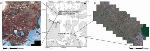
The mid-Arctic site is located on Boothia Peninsula in the Kitikmeot region of Nunavut within the Lord Lindsay River watershed, west of Sanagak Lake (SL; 70°1′ N, 93°44′ W; Figure 1b). The Lord Lindsay River to the south and a large tributary river to the north confined the sampling for this study. Active layer depth varies between 0.5 and 1 m. In 2006, the mean temperature for the study period (15 July to 4 August) was 9.5°C with a total precipitation of 6.6 mm. The long-term July climatic averages from 1986 to 2005 for temperature and rainfall at the closest meteorological station in Taloyoak (and the former Spence Bay) were 8.28°C and 19.90 mm (Environment Canada 2019). The study site is in Bioclimatic Zone C, characterized by a mean July temperature of 5°C to 7°C and dominated by sedges and small branching shrubs (Walker et al. 2002). The vegetation classification for the area is P1: prostrate dwarf shrub, herb tundra (Walker et al. 2005).

Vegetation types

At each study site, three tundra vegetation types were identified along a summer season soil moisture gradient (dry, mesic, and wet) with replicate plots established for each type. These vegetation types were characterized by Atkinson and Treitz (2012), where species composition, percentage vegetation cover (PVC), aboveground biomass, and gravimetric soil moisture (GSM) were quantified at peak growing season. The Circumpolar Arctic Vegetation Map (Walker et al. 2005) was applied to describe the vegetation classifications for the CBAWO and SL (Table 1). The dry vegetation types (dry tundra, DT) at the CBAWO and SL are most closely related to P1: prostrate dwarf shrub and herb tundra (Walker et al. 2005). At the CBAWO and SL, microscale topographic features (e.g., frost cracks) create moisture gradients that influence the pattern and distribution of vegetation. Plant growth is limited to these frost cracks and depressions where wind speeds are reduced, thereby decreasing rates of evaporation and facilitating the accumulation of plant detritus (organic matter), which increases soil water-holding capacity and nutrient availability (Oberbauer and Dawson 1992). Though they are similar, the DT at each site is distinct. Although the predominant exposed surface material for DT at the CBAWO and SL is glacial till (~60 percent), the secondary cover types vary (CBAWO, bryophytes [18.5 percent]; SL, Dryas spp. [18.4 percent]), and the overall PVC for each DT is 25.4 and 30.4 percent, respectively. The CBAWO is distinct in that Papaver radicatum is a major species in the DT. The CBAWO dry sites are referred to as dry P. radicatum and till tundra, whereas SL sites are referred to as dry Dryas spp. and till tundra (Atkinson and Treitz 2012). The mesic tundra (MT) sites at the CBAWO and SL—for example, mesic Nostoc tundra (G1, rush/grass, forb, cryptogam tundra) and mesic Dryas spp. tundra (G2, graminoid, prostrate dwarf shrub, forb tundra), respectively—are similar in terms of total PVC (101.7 and 80.4 percent). However, the primary cover at the CBAWO is Nostoc commune (48.6 percent), a nitrogen-fixing cyanobacteria that forms a black crust on the soil (Liengen and Olsen 1997), typically found in association with bryophyte species and Salix arctica. In contrast, Dryas spp. is found in the majority of SL sites in varying percentages but rarely at the CBAWO. Dryas spp. (46.0 percent) and Carex spp. (10.6 percent) were the primary and secondary cover types of the SL MT sites, along with extensive Saxifraga oppositifola. The wet vegetation types (wet tundra, WT) at the CBAWO and SL were extremely similar in species composition and PVC. At the CBAWO and SL, WT sites (most closely related to W1: sedge/grass, moss wetland) are often located in areas exhibiting high levels of soil moisture throughout the growing season, often due to the proximity of large upslope snow banks. The total PVC for these sites was 154 percent, due to the layering of vegetation, with Sphagnum spp. (69.3 percent) and Eriophorum spp. (47.5 percent) comprising the main cover types. Dryas spp. was present in some SL WT sites. Replicate vegetation plots (100 m × 100 m) were selected for each vegetation type at both sites (CBAWO [n = 7]: two DT, two MT, three WT; SL (n = 5): one DT, two MT, two WT).

Table 1. Classification summary for dry, mesic, and wet vegetation types at the Cape Bounty Arctic Watershed Observatory (CBAWO) and Sanagak Lake (SL)

	CBAWO			SL
Ecosystem	Dry P. radicatum and till tundra	Mesic Nostoc tundra	Wet sedge tundra	Dry Dryas spp. and till tundra	Mesic Dryas spp. tundra	Wet sedge tundra
Soil moisture (%)	17.1	37.3	123.9	17.2	41.2	123.3
Percent vegetation cover (%)	50.2	101.7	154.0	30.4	80.4	144.8
Bryophyte cover (%)	11.6	57.7	88.0	8.8	1.3	59.7
Graminoid cover (%)	0.0	21.8	71.4	0.5	16.8	38.1
Shrub cover (%)	4.3	0.0	2.9	25.0	57.9	32.1
Lichen cover (%)	11.4	9.0	1.6	1.0	1.1	1.4
Forb cover (%)	0.7	4.1	0.8	0.3	1.2	0.0
Biomass (g m^−2)	348.5	1,477.3	1,561.6	298.2	521.7	825.6
Cover (%)	26.9	89.9	141.0	41.0	87.0	131.3
Primary cover	Till	Nostoc commune	Sphagnum spp.	Till	Dryas spp.	Sphagnum spp.
Secondary cover	Mosses	Mosses	Eriophorum spp.	Dryas spp.	Carex spp.	Eriophorum spp.
Indicator species	P. radicatum	Nostoc commune	Eriophorum spp.	n/a	Dryas spp.	Eriophorum spp.
Bioclimatic class (Walker et al. 2005)	P1	G1	W1	P1	G2	W1

Notes.P1 –  prostrate dwarf shrub and herb tundra; G1 – rush/grass, forb, cryptogam tundra; G2 – graminoid, prostrate dwarf shrub, forb tundra; W1 – sedge/grass, moss wetland.

Environmental measurements

Soil temperature, GSM, air pressure, air temperature, and precipitation were all measured during the sampling period. Soil temperatures were recorded (using the Thermor stem thermometer model PS100, Themor Limited, Newmarket, Ontario, Canada) at 5 and 10 cm depths in the soil/organic layer simultaneously with each CO₂ exchange measurement at three random positions adjacent to each chamber. GSM was determined on each measurement day by collecting three 5-cm-depth, 5.3-cm-diameter soil cores. These samples were weighed wet in the field and returned to the lab for oven drying at approximately 110°C for 48 hours; GSM was determined as the mass of water expressed on a volumetric basis. Air pressure was measured during each CO₂ measurement cycle with a handheld Kestrel weather meter (Kestrel Meters, Sylvan Lake, Michigan).

CO₂ exchange measurements

Static chambers (~35 cm height, 285 cm² area, ~8.7 L) equipped with a Vaisala GMP343 infrared gas analyzer (Vaisala, Vantaa, Finland) were used to make CO₂ exchange measurements. The chamber was also instrumented with a Vaisala HMP75 temperature and relative humidity sensor (Vaisala) to adjust for relative humidity variation in real time. Temperature corrections were done manually using the ideal gas law during postprocessing (Equation (1)(1) $n=C\left(\frac{\rho }{R\tau }\right)\left(\frac{\nu }{\mathrm{A}}\right)/5$(1) )(1) $n=C\left(\frac{\rho }{R\tau }\right)\left(\frac{\nu }{\mathrm{A}}\right)/5$(1) . The chamber was also fitted with a pressure equalization vent and a small circulation fan (Hutchinson and Mosier 1981). The chamber was allowed to achieve equilibrium with ambient CO₂ and temperature prior to any measurement. CO₂ concentrations, temperature (T), and relative humidity (RH) were logged as the average value for each sensor every 5 seconds for a 5-minute period. NEE measurements were derived from measures using the transparent chamber. After NEE measurements were completed, the chamber was removed, allowed to return to ambient conditions, fitted to the collar, and covered with an opaque hood to collect “dark” readings (ER).

A PVC collar (inner diameter 19.9 cm, height ~15 cm) was inserted at the center of each plot at a minimum of 24 hours prior to the initial sampling, but in most cases this period was 24 to 72 hours before sampling and conforms with other studies of arctic gas exchange (Stewart et al. 2013). The collars were then left in place and revisited during the growing season. The collars were inserted after cutting rings into the soil and vegetation; all attempts were made not to damage vegetation or root systems within the collar. Approximately 4 cm of the collar remained above the surface and was fitted with a rubber gasket to create an airtight seal between the collar and the flux chamber. In dry plots, where there was extensive exposed soil, two collars were inserted: one in bare soil and one within a vegetated area. CO₂ exchange measurements at the CBAWO began on 5 July 2006 and continued until 30 July 2006, resulting in six to seven sampling cycles per plot. At SL, measurements were collected from 18 July 2006 to 3 August 2006, resulting in four to five sampling cycles per plot. Each plot was sampled systematically every two to three days. Sampling began at 8 a.m. and was repeated every four hours (8 a.m., 12 p.m., 4 p.m., 8 p.m.) for a 12-hour cycle, resulting in four measurements per plot per sample day.

CO₂ flux calculations

CO₂ flux rates were calculated using a custom Matlab script (Matlab 2012). All CO₂ concentrations were converted from CO₂ concentration (ppm) to micromoles of CO₂ per square meter using the ideal gas law after Shaver et al. (2007):

(1) $n=C\left(\frac{\rho }{R\tau }\right)\left(\frac{\nu }{\mathrm{A}}\right)/5$(1)

where n is the converted concentration (μmol m⁻²), c is the concentration of CO₂ (ppm), ρ is air pressure (hPa), R is the ideal gas constant (0.08314 hPa m³ mol⁻¹ K⁻¹), τ is the temperature (K), ν is the volume of the chamber after insertion into the collar (m³), and Α is the projected horizontal surface area of the chamber (m²). Because of the possibility of sampling artifacts at the beginning and ending of each measurement cycle, the rate was calculated using an iterative multiple regression search algorithm, which searches for a linear set of readings that create the best possible coefficient of determination (R²) for the longest time period (minimum 60 seconds) with the highest level of significance. The slope of this linear regression was then recorded as the flux rate (μmol CO₂ m⁻² s⁻¹) for each measurement. Finally, GEE was calculated as

(2) $\mathrm{G}\mathrm{E}\mathrm{E}=\mathrm{N}\mathrm{E}\mathrm{E}-\mathrm{E}\mathrm{R}$(2)

Hence, we adopt the sign convention that net CO₂ uptake to the vegetation type is negative, whereas net CO₂ flux to the atmosphere is positive (Dagg and Lafleur 2011).

Satellite remote sensing data

IKONOS multispectral data (4 m spatial resolution) were acquired for the CBAWO on 22 July 2004 and 2 August 2008 and for SL on 23 July 2001. The 2004 and 2001 images respectively for the CBAWO and SL were used for modeling CO₂ exchange, and the 2008 image of the CBAWO was used for model validation. The spectral characteristics of the three images are similar, with almost identical time of year, time of day, and solar angle. Though these images do not correspond with the field sampling year, it is assumed that they are representative of the peak growing season. Image bands (blue: 0.45–0.52 μm; green: 0.51–0.60 μm; red: 0.63–0.70 μm, and near-infrared [NIR]: 0.76–0.85 μm) were calibrated to top of atmosphere reflectance following procedures outlined by Taylor (2005). The images were geo-referenced with an overall root mean square error (RMSE) of less than 3 m horizontally. NDVI data were derived from the difference in reflectivity of the land cover in the NIR band, where vegetation structure reflects strongly, and the red (R) band, where vegetation absorbs strongly as a function of chlorophyll concentration. NDVI for each image pixel was calculated as follows:

(3) $\mathrm{N}\mathrm{D}\mathrm{V}\mathrm{I}=\left(\mathrm{N}\mathrm{I}\mathrm{R}-\mathrm{R}\right)/\left(\mathrm{N}\mathrm{I}\mathrm{R}+\mathrm{R}\right)$(3)

NDVI data were extracted from individual sample locations; for example, sample site NDVI data were interpreted from adjacent cells (n = 8) using bilinear interpolation, which minimizes the effects of misregistration errors (Fuchs et al. 2009).

Statistical analyses

Site and vegetation type differences

Collecting flux data four times per day provided a more robust daily average flux value compared to single measurements. We explored possible vegetation effects on diel fluctuations using two-way repeated measures analysis of variance (ANOVA) with vegetation type and time of day as between-subjects factors. The interaction between vegetation type and time of day was nonsignificant (p = .893), allowing us to compute a daily average flux for subsequent analyses. We used two-way repeated measures ANOVA to then examine differences among sites (n = 2) and vegetation type (n = 3) as well as seasonal variability using time (dates of measurements) as the within-subjects variable. Average values were tested for homogeneous variance (Levene’s) and normality (Shapiro-Wilk) and found to satisfy both assumptions in most cases (p > .05).

Regression modeling with environmental variables

Stepwise multiple linear regression was used at each site to test the importance of averaged environmental variables on mean 12-hour daytime CO₂ fluxes for each vegetation type. Simultaneous measures of air temperature, 5-cm and 10-cm depth soil temperatures, daily soil moisture, and PAR were examined. Significance of .10 was used for variable selection. Data were tested for normality using Shapiro-Wilk’s test (n < 50) and for homogeneous variance using Levene’s test. The data did not satisfy these assumptions; thus, values were transformed using a natural log transformation on scaled fluxes. Data were also tested for multicollinearity using variance inflation factor values.

Modeling CO₂ with NDVI

Linear bivariate regressions were generated with NDVI as the independent variable and the averaged seasonal CO₂ flux values as the dependent variable. Though NDVI would be considered a function of the biophysical variables, the reversal of the variables allows for the calculation of spatial models (Shippert et al. 1995; Laidler, Treitz, and Atkinson 2008). With regression equations derived for each flux component and for each study site, we used analysis of covariance (ANCOVA) to determine whether relationships between NDVI and the component fluxes differed significantly across sites. If no significant difference in the relationships between NDVI and the components fluxes is found—for example, the empirical models exhibit equal slopes $\left(H_0:{\beta }_{1CB}={\beta }_{1SL}\right)$ and equal intercepts $(H_0:{\beta }_{0CB}={\beta }_{oSL})$—the data can be pooled from each independent site to derive a single model $\left(Y={\beta }_0+{\beta }_{1}X+\mathrm{E}\right)$ to describe the relationship between NDVI and a component flux.

Model validation

Statistical model validation was based on data collected at the CBAWO during the 2008 summer season. CO₂ and environmental measurements were collected for six of the vegetation plots (two DT, two MT, and two WT) sampled in 2006 and an additional five vegetation plots not previously sampled (two DT, two MT, one WT) for a total of four DT, four MT, and three WT vegetation plots. CO₂ exchange measurements were made between 24 June and 4 August 2008. Each plot was sampled weekly during weeks 1, 2, 5, and 6 and biweekly during weeks 3 and 4. The only significant difference in the sampling methodology in 2008 from 2006 was that only peak daytime fluxes were measured in 2008, whereas 12-hour samples (every 4 hours) were collected in 2006. All data collection and processing of the 2008 data (CO₂ flux measurements, environmental data collection and measurements, and image preprocessing) was performed in the same manner as for the 2006 data. All statistical analyses were conducted in SPSS Version 25.0 (IBM Corp 2017).

Results

CO₂ exchange

Based on results from the two-way repeated measures ANOVA, site had no significant effect on any of the CO₂ fluxes (Table 2). Across all sites, rates of ER were generally highest in the WT sites and lowest in the DT sites (p < .1; Table 2, Figure 2). Similarly, GEE was also generally highest in the WT and lowest in the DT sites. These patterns were consistent across both study sites (i.e., SL and the CBAWO); there were no significant Site × Vegetation type interactions (Table 2). Rates of ER were generally consistent over the different sample dates at both study sites (Table 2; Figure 2), but they did exhibit different (p = .02) patterns in ER over time (Figure 2). GEE varied significantly over time (Table 2, Figure 2), showing strong seasonal patterns at the CBAWO compared to SL (Figure 2).

Table 2. p Value results from two-way repeated measures analysis of variance (ANOVA) testing the effect of site (Cape Bounty Arctic Watershed Observatory versus Sanagak Lake), vegetation type (dry tundra versus mesic tundra versus wet tundra), and time on gross ecosystem exchange (GEE), ecosystem respiration (ER), and net ecosystem exchange (NEE). Numbers within the brackets signify degrees of freedom between and within groups respectively

Flux	Site(1,7)	Veg.(2,7)	Site × Veg.(2,7)	Time(3,21)	Time × Site(3,21)	Time × Veg.(6,21)
GEE	0.65	0.004	0.32	0.06	0.22	0.89
ER	0.89	0.097	0.63	0.22	0.02	0.73
NEE	0.86	0.078	0.36	0.27	0.77	0.50

Figure 2. Mean daytime carbon dioxide (CO₂) exchange rates for the Cape Bounty Arctic Watershed Observatory (CBAWO): (a) dry tundra (DT), (b) mesic tundra (MT), (c) wet tundra (WT); and Sanagak Lake (SL): (d) DT, (e) MT, and (f) WT. Positive CO₂ exchange rates indicate CO₂ loss to the atmosphere, whereas negative signed values indicate CO₂ gain to the vegetation type. Error bars represent standard error of the mean

Given the small overall time differences, we compared vegetation types and study sites using linear interpolation of each vegetation type flux rate to get one representative flux for the entire growing season (Figure 3). ER rates at SL and the CBAWO were similar in each of their comparable vegetation types. The WT had the highest GEE, and it was higher at the CBAWO compared to SL (Table 3, Figure 3). As a result, WT was the only vegetation type demonstrating net uptake (e.g., negative NEE) across the sampling period at the CBAWO. The MT at the CBAWO, though it was a modest source, had a somewhat lower GEE rate than MT at SL, where it was a modest sink. At both study sites, DT proved to be a source of CO₂ across the growing season even though GEE was stronger at the CBAWO than at SL.

Table 3. Averaged carbon dioxide (CO₂) flux rates for the duration of the study period (mmol CO₂ m^-2 s^-1) with standard error in parentheses (by vegetation type and geographic location)

	GEE		ER		NEE
Vegetation type	CBAWO	SL	CBAWO	SL	CBAWO	SL
DT	–0.58 (±0.11)	0.02 (±0.14)	0.03 (±0.08)	0.66 (±0.14)	0.74 (±0.05)	0.64 (±0.09)
MT	–1.09 (±0.13)	–1.27 (±0.13)	0.15 (±0.11)	–0.24 (±0.12)	1.25 (±0.08)	1.04 (±0.06)
WT	–2.15 (±0.14)	–1.51 (±0.15)	–0.87 (±0.12)	–0.21 (±0.15)	1.29 (±0.09)	1.31 (±0.06)

Notes. Dry tundra (DT), mesic tundra (MT), wet tundra (WT), gross ecosystem exchange (GEE), ecosystem respiration (ER), net ecosystem exchange (NEE), Cape Bounty Arctic Watershed Observatory (CBAWO), Sanagak Lake (SL).

Figure 3. Interpolated total daily carbon dioxide (CO2) exchange rates for dry tundra (DT), mesic tundra (MT) and wet tundra (WT) at the Cape Bounty Arctic Watershed Observatory (CBAWO) and Sanagak Lake (SL) during the study period

Regression modeling with environmental variables

Daily average ecosystem carbon fluxes were generally poorly correlated with daily average environmental variables, generally explaining roughly 50 percent of the variability in each CO₂ flux (Table 4). Temperature (air or soil) was generally the most important predictor for the daily fluxes regardless of vegetation type and was a significant variable in most of the multiple regression models. Soil temperature predicted rates of ER significantly, explaining 60 to 70 percent of the variability in ER at both sites. Environmental variables were generally poor predictors of NEE (Table 4). It should be noted that some multiple regressions had a small sample size (e.g., SL-DT, where n = 4).

Table 4. Multiple linear regression analysis for plot-level daily averaged carbon dioxide (CO₂) exchange rates in relation to averaged environmental variables (p < .05)

Site	Flux	Type	Predictor	Slope	R^2 adjusted	RMSE	F	p Value	df
CBAWO	GEE	DT	Air temperature	0.65	0.595	0.10	15.69	.003	1, 9
	ER	DT	Air temperature	−0.45	0.542	0.08	12.81	.006	1, 9
		MT	Soil moisture, air temperature	4.02	0.651	0.06	9.38	.010	2, 7
	NEE	MT	Photosynthetically active radiation (PAR)	2.84	0.331	0.12	5.46	.048	1, 8
SL	ER	DT	Soil temperature (10 cm)	0.24	0.996	0.00	729.49	.001	1, 2
		MT	Air temperature	0.42	0.212	0.07	4.77	.048	1, 13
		WT	Soil temperature (10 cm)	0.42	0.676	0.04	19.77	.002	1, 8
	NEE	MT	Soil temperature (10 cm)	−1.23	0.259	0.09	5.890	.030	1, 13

Notes. Dry tundra (DT), mesic tundra (MT), wet tundra (WT), gross ecosystem exchange (GEE), ecosystem respiration (ER), net ecosystem exchange (NEE), Cape Bounty Arctic Watershed Observatory (CBAWO), Sanagak Lake (SL)

Modeled CO₂ exchange using NDVI

Bivariate linear regressions were derived to examine relationships between NDVI and average seasonal daytime GEE, ER, and NEE at the CBAWO (n = 7) and SL (n = 5). All regressions were significant (p < .01; Table 5). The ANCOVA results for each of the regression equations indicates that none of the slopes were significantly different between the two study sites (p < .05) and thus the fluxes vary with NDVI equally across the sites. Given that the regression equations for the CBAWO and SL are statistically similar, the data were combined into a single equation (n = 12) for each flux and applied to both sites (Figure 4, Table 5). NEE was the hardest to predict from NDVI alone, whereas NDVI explained over 70 percent of the variation in both GEE and ER (but not for all vegetation types (Table 5).

Table 5. Bivariate linear regression $\left(Y={\beta }_0+{\beta }_{1}X+\mathrm{E}\right)$ and analysis of covariance (ANCOVA) results for carbon dioxide (CO₂) exchange components gross ecosystem exchange (GEE), ecosystem respiration (ER), and net ecosystem exchange (NEE) with the normalized difference vegetation index (NDVI) for the Cape Bounty Arctic Watershed Observatory (CBAWO) and Sanagak Lake (SL)

						ANCOVA
CO2 flux (Y)	Site	Slope (${\beta }_1$)	Intercept (${\beta }_0$)	R^2	RMSE	Slope (p value)	Intercept (p value)
GEE	CBAWO	−8.41	0.04	0.64	0.23	.695	.528
	SL	−7.72	0.15	0.72	0.14
	Combined	−8.15	0.10	0.65	0.48
	Validation	−7.85	0.15	0.48	0.96	.932	.748
	Combined	−8.05	0.13	0.54	0.70
ER	CBAWO	3.97	0.58	0.66	0.06	.391	.199
	SL	4.07	0.38	0.94	0.02
	Combined	4.03	0.49	0.70	0.21
	Validation	3.81	0.43	0.75	0.26	.847	.337
	Combined	3.97	0.46	0.73	0.23
NEE	CBAWO	−4.28	0.57	0.33	0.14	.485	.916
	SL	−3.25	0.36	0.48	0.08
	Combined	−3.87	0.48	0.35	0.42
	Validation	−3.85	0.54	0.26	0.75	.994	.815
	Combined	−3.91	0.51	0.30	0.57

Figure 4. Combined bivariate linear regressions for carbon dioxide (CO₂) exchange rates: gross ecosystem exchange (GEE), ecosystem respiration (ER), and net ecosystem exchange (NEE)

Model validation

CO₂ flux measurements and NDVI values for 2008 (n = 11) were examined using the same methods of bivariate linear regression as discussed above and were all found to be significant (p < .01; Table 5). The regression equations for each flux rate were similar to the 2006 pooled data, though the R² values were lower. The lower R² values can be attributed to fewer samples with a greater variability (one at peak of day as opposed to four daily samples). ANCOVA was performed to test the similarity of the 2008 validation equations with the 2006 pooled data. Again, both equations showed parallelism (similar slopes) and similar intercepts, indicating that the 2008 validation equations are statistically similar to the 2006 pooled data.

The NDVI model for ER had the lowest percentage error (6.4 percent) of all of the CO₂ fluxes (Table 6). ER is a combination of autotrophic and heterotrophic respiration, and the ability for a spectrally based model to predict this flux illustrates the integration of various environmental variables within the NDVI signal. In a 1:1 comparison of actual versus NDVI predicted ER flux, WT tends to be overpredicted, whereas MT is underpredicted (Figure 5). The error estimates for the GEE model were moderate at 27.2 percent (Table 6). In a 1:1 comparison for the GEE regression model, the situation is reversed from ER, where MT was underpredicted and WT was slightly overpredicted (Figure 5). For the NEE model, which had the largest percentage error (57.6 percent; Table 6), we see that DT is an overpredicted source, WT is an overpredicted sink, and MT is highly variable (Figure 5). The reasoning for this may be that with NEE exhibiting such small values (i.e., close to zero), there is a greater potential for error. Alternatively, with the NDVI models for ER and GEE, it is possible to derive NEE from the models, thereby potentially reducing the overall error.

Table 6. Normalized difference vegetation index (NDVI) model-based carbon dioxide (CO₂) exchange rates for the Cape Bounty Arctic Watershed Observatory (CBAWO) and Sanagak Lake (SL)

Site	Area (km^2)	Flux	Mg CO2 day^−1	SMAPE estimate (%)
CBAWO	80.74	GEE	−141.16	27.2
		ER	244.77	6.4
		NEE	64.19	57.6
SL	74.32	GEE	−338.14	27.2
		ER	305.77	6.4
		NEE	−36.76	57.6

Notes. Gross ecosystem exchange (GEE), ecosystem respiration (ER), net ecosystem exchange (NEE), Symmetric mean absolute percentage error (SMAPE).

Figure 5. One-to-one comparisons of actual calibration values and normalized difference vegetation index (NDVI) modeled values for gross ecosystem exchange (GEE), ecosystem respiration (ER), and net ecosystem exchange (NEE)

Watershed-scale estimates of CO₂ exchange

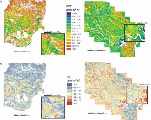
The regression equations generated for the 2006 data and validated with the 2008 data were applied to the NDVI images of SL (2001) and the CBAWO (2004), generating spatially explicit estimates of CO₂ flux for each site (Figure 6). Based on CO₂ exchange rates per pixel, summary statistics were calculated for each flux model, resulting in estimates of total CO₂ exchange per day during the summer peak season (Table 6). Symmetric mean absolute percentage error (SMAPE) was selected as a non-scale-dependent estimate of error for the regression equations’ relative error statistics. SMAPE is a variation on the mean absolute percentage error (MAPE) and is calculated using the average of the absolute value of the actual and predicted values in the denominator. This statistic is preferred when low values are problematic because they could skew the overall error rate higher (Chen et al. 2009; Tofallis 2014). Based on this model, the CBAWO is an overall source of CO₂ (64.19 Mg CO₂ day⁻¹) and SL is an overall sink (–36.8 Mg CO₂ day⁻¹).

Figure 6. Spatially-explicit models of (a) gross ecosystem exchange (GEE) and (b) ecosystem respiration (ER) for the Cape Bounty Arctic Watershed Observatory (CBAWO) (left) and Sanagak Lake (SL) (right). White indicates no flux data

Discussion

Variability across vegetation types and sites

Though numerous studies have examined carbon dynamics across vegetation types distributed along moisture gradients, few have studied these responses across bioclimatic zones, and fewer have done so in the high Arctic (Wüthrich, Moller, and Thannheiser 1999; Emmerton et al. 2016). Recent pan-Arctic studies have not examined vegetation types north of Bioclimatic Zone C (Shaver et al. 2013). Within each of our sites, environmental variables differed by vegetation type. However, soil temperature (5 and 10 cm depth), GSM, and PVC were not statistically different in comparable vegetation types between the CBAWO and SL despite the large latitudinal and bioclimatic difference. This lack of variability in environmental conditions between sites is interesting because species composition differed greatly between the CBAWO and SL in each of the three corresponding vegetation types. A major species compositional difference between the CBAWO and SL was the dominance of the shrub Dryas spp. at SL, where it was found in all vegetation types, whereas shrub cover at the CBAWO was limited. Additionally, there was a greater abundance (e.g., cover) of bryophytes at the CBAWO than at SL, except for the WT. These similarities were confirmed spectrally, in that NDVI values for all vegetation types at the CBAWO and SL were similar.

Temporal variation in CO₂ fluxes within a given vegetation type is important. There were no statistically significant variations in GEE, ER, or NEE over the sampling periods at either site, with the exception of ER in MT and WT at SL. The variation in ER rates in these vegetation types appears to be linked to unseasonably cool temperatures during a specific ten-day period (temperature decreased with the ER rate for MT and WT). These findings support Hypothesis 1 for the CBAWO: Daytime CO₂ exchange rates (GEE, ER, NEE) within DT, MT and WT are consistent through the peak summer growing season. On the other hand, the results cannot definitively support Hypothesis 1 for SL, although the majority of sites and CO₂ fluxes exhibited consistency (e.g., no statistically significant differences) when seasonal conditions prevail.

Although CO₂ flux studies for the high Arctic are limited, Wüthrich, Moller, and Thannheiser (1999) also noted that there was no statistical variation within DT, MT, or WT during a study on West Spitzbergen (78°22′ N; 12°44′ E; through early- and mid-season plant activity [8–26 July]). Environmental conditions during the growing season at the West Spitzbergen coastal site are similar to the CBAWO with low cloud and frequent fog. Conversely, studies in the mid- and low Arctic have noted extensive variability within vegetation types in terms of GEE, ER, and NEE fluxes (Nobrega and Grogan 2008). The greatest variability is observed during the early and late growing season (e.g., shoulder seasons), coincident with the greatest temperature fluctuations (Nobrega and Grogan 2008). This contradiction with respect to vegetation type may be a product of latitude and its impact on PAR and temperature. The high Arctic climate is cooler, with a short growing season through the summer months, compared to the mid- and low Arctic. Hence, increases in temperature and PAR may have a greater impact on the processes connected to CO₂ exchange rates at more southern sites. Regression modeling in this study indicated that air or soil temperature were the best predictors for the most successfully modeled fluxes. It has been shown that temperature and soil moisture have been key predictors of NEE, GEE, and ER for high Arctic DT, MT, and WT (Emmerton et al. 2016). The results of this study may be dependent on the conditions at these sites being relatively stable during the measurement period, so additional seasons should be examined.

CO₂ exchange model

Extensive research has been devoted to defining plant functional groups for the modeling of CO₂ exchange (Hobbie and Chapin 1996; Chapin and Shaver 1996; Callaghan et al. 2005; Wullschleger et al. 2014). This method of modeling requires detailed knowledge of vegetation distribution, which can be derived from remotely sensed data at a range of spatial resolutions (Shaver et al. 2007). The spatial model for CO₂ exchange in this study was independent of vegetation type and based solely on the spectral reflectance characteristics of vegetation. The NDVI model developed here demonstrates a functional convergence of vegetation types, in that the model is independent of species composition or functional type and builds on the relationships between vegetation cover, structure, and spectral reflectance (Shaver et al. 2007).

To examine Hypothesis 2, which posits that CO₂ exchange rates illustrate functional convergence and are captured in the NDVI data, we need to examine a number of ecological components. First, vegetation types, based on a soil moisture gradient at the CBAWO and SL, were composed of different species and functional groups, yet there was no statistically significant difference in CO₂ exchange across vegetation types (DT, MT, and WT) and site (CBAWO and SL). This may in large part be due to NDVI being strongly correlated with biogeophysical variables (e.g., PVC, aboveground biomass, leaf area, and soil moisture; Shippert et al. 1995; Walker, Auerbach, and Shippert 1995; Rees, Golubeva, and Williams 1998; Stow et al. 2004; La Puma, Philippi, and Oberbauer 2007; Laidler, Treitz, and Atkinson 2008; Atkinson and Treitz 2013). Hence, the NDVI values for similar vegetation types at both sites were not statistically different from one another. When NDVI was used to model carbon fluxes, the coefficient of determination (R²) illustrated that NDVI explained between 66 and 94 percent of the variation in GEE and ER at the CBAWO and SL. All regression equations confirmed coincidence, indicating that they were statistically similar and could be combined into one equation for both sites, thereby supporting Hypothesis 2. NEE was the weakest of the regression models at both sites; NEE was relatively low, because it was balanced by opposing GEE and ER values. However, NDVI did explain 35 percent of the variation in NEE at both sites. The results suggest that a simple model based on NDVI can be applied to accurately predict carbon exchange processes.

Hypothesis 3 states that NDVI alone can model landscape-scale CO₂ exchange rates at two independent sites. This hypothesis has been confirmed, in that all regression equations were coincidental and allowed one equation for each component, regardless of site, and that 35 to 70 percent of the variations in GEE, ER, and NEE rates were explained by NDVI. Additionally, the application of independent data collected in 2008 at the CBAWO reinforces the robust nature of these equations, because they were statistically similar to the pooled data. Thus, these models contribute to our understanding of functional convergence for CO₂ flux models.

Functional convergence models have been explored for the low Arctic (Shaver et al. 2007), and pan-Arctic models for NEE have been developed recently (Shaver et al. 2013). These models have had success with modeling NEE with R² values of 0.70 (RMSE = 1.16) for high Arctic sites (though no sites were at the latitude of this study). These models are multiple regression equations, requiring air temperature, PAR, and LAI. LAI values are derived from NDVI as a primary model input (Shaver et al. 2013). LAI is a quantifiable and straightforward measure for vascular plants and is preferable, at times, to other, more abstract variables (Street et al. 2007). Furthermore, LAI is estimated from NDVI using empirically based models (van Wijk and Williams 2005). However, NDVI values have been shown to vary based on sensor, so LAI models are often sensor specific (Laidler, Treitz, and Atkinson 2008). Additionally, it is difficult to incorporate nonvascular plant cover, an important component in high Arctic tundra CO₂ exchange, in LAI models (Shaver et al. 2007). For this research, a simple bivariate model with NDVI was optimal, in that it alone captures the spectral difference between red and NIR reflectance of all aboveground biomass. The results of the simpler bivariate models for GEE and ER developed here have similar R² values (0.70 and 0.65) and lower RMSE (0.21 and 0.48). The benefit of this bivariate model is that future estimates can be generated through the acquisition of new satellite imagery and not require in situ data, such as PAR and air temperature.

Study limitations and recommendations

Although the NDVI models developed here do explain a large portion of variance in CO₂ exchange rates (33 to 94 percent), there is additional variance left unexplained. However, this study illustrates that NDVI can be used quite simply to model CO₂ component fluxes, which can allow for the estimation of CO₂ exchange across large spatial scales without the need for additional in situ measures (e.g., soil moisture and temperature). It is anticipated that the inclusion of additional variables, such as PAR, air temperature, and water table depth, will improve model development and predictions (Oechel et al. 1998; Street et al. 2007; Huemmrich et al. 2010; Olivas et al. 2010; Virkkala et al. 2018). Modeling peak growing season CO₂ dynamics can be valuable for understanding the ongoing changes to these processes with climate warming; however, more and more research is showing the importance of studying Arctic systems during non-growing seasons to fully understand the trajectory of change. Laboratory incubation studies have found evidence of microbial activity and subsequent CO₂ release at −10°C (Mikan, Schimel, and Doyle 2002). In situ evidence of CO₂ release under snowpack during the winter and spring periods has also been observed in the Alaskan Brooks Range, and these CO₂ effluxes were quite variable across different vegetation types (Fahnestock et al. 1998). Though NDVI models cannot be used accurately to model non-growing season CO₂ due to winter solar conditions, knowledge of the relationships between CO₂ dynamics and other influencing factors like temperature, moisture, and soil carbon quality can be included in these models to better develop our understanding of annual landscape-scale CO₂ processes.

Conclusions

A warming climate in the Arctic impacts terrestrial ecosystems directly and further complicates our understanding of how Arctic terrestrial ecosystems behave with respect to carbon and energy exchange (as a net source or sink for carbon). In a changing climate, we need to model and monitor CO₂ exchange rates throughout the Arctic at a variety of spatial and temporal scales (Virkkala et al. 2018). The application of high spatial resolution remote sensing data makes it possible to model CO₂ exchange rates where limited environmental data exist by capturing the heterogeneity of biophysical properties of tundra ecosystems based on their spectral reflectance. The ongoing challenge with intermediate and high spatial resolution data is the value that a single image can provide regarding processes occurring over longer timescales. Here, we have demonstrated that there was no statistically significant variation in GEE, ER, or NEE during the three- to five-week peak growth period at two independent study sites. These results illustrate that a single image captured within that time frame can be used to extrapolate temporally across the peak photosynthetic period. Additionally, the fact that GEE and ER can be predicted reasonably well for DT, MT, and WT in the mid- and high Arctic using NDVI demonstrates a strong functional convergence for these vegetation types.

This study examines statistical significance, which is not always related to ecological significance. Hence, field data and image data from additional years and study sites will further refine these models for application across broader environmental gradients of the Arctic. Further research is required to better understand the spatial and temporal variability of soil moisture, soil pH, nutrient availability, PAR, and their influences on carbon exchange processes. The majority of studies examine arctic vegetation types during the time-limited summer season, often due to logistical limitations, with only limited studies examining the shoulder seasons of spring and fall (Fahnestock et al. 1998; Nobrega and Grogan 2008; Sullivan et al. 2008; Commane et al. 2017). Focused research into arctic vegetation processes and how they relate to remotely sensed data will improve our ability to predict and understand the impacts of climate change over time.

Acknowledgments

The authors thank Kimberly Molina, Dana McDonald, Eva Fisher, and Shanley Thompson for their assistance collecting field data. Special thanks to Dr. Paul Grogan for his advice related to CO₂ sampling and chamber design. Thank you to Dr. Scott Lamoureux, director of the Cape Bounty Arctic Watershed Observatory (CBAWO), for his guidance.

Disclosure statement

No potential conflict of interest was reported by the authors.

Additional information

Funding

This work was supported by the Polar Continental Shelf Program with travel assistance received from the Department of Indian Affairs and Northern Development and the Northern Scientific Training Program. Funding was provided by the Natural Sciences and Engineering Research Council of Canada (NSERC) in the form of Postgraduate Doctoral Scholarship to David Atkinson and a Discovery Grant (No. 388581) to Dr. Paul Treitz.

References

- Arctic Monitoring and Assessment Program (AMAP). 2017. Snow, water, ice, and permafrost in the Arctic (SWIPA). Norway: Oslo.
- Atkinson, D. M., and P. Treitz. 2012. Arctic ecological classifications derived from plant community and satellite spectral data. Remote Sensing 4 (12):3948–71. doi:https://doi.org/10.3390/rs4123948.
- Atkinson, D. M., and P. Treitz. 2013. Modelling biophysical variables across an arctic latitudinal gradient using high spatial resolution remote sensing data. Arctic, Antarcitc, and Apline Research 45 (2):161–78. doi:https://doi.org/10.1657/1938-4246-45.2.161.
- Bintanja, R. 2018. The impact of Arctic warming on increased rainfall. Nature Scientific Reports 8 (1):16001. doi:https://doi.org/10.1038/s41598-018-34450-3.
- Bliss, L. C., and N. V. Matveyeva. 1992. Circumpolar Arctic vegetation. In Arctic ecosystems in a changing climate – An ecophysiological perspective, ed. S. F. Chapin, R. L. Jeffries, J. F. Reynolds, G. R. Shaver, J. Svoboda, and E. W. Chu, 59–89. San Diego: Academic Press Inc.
- Boelman, N. T., M. Stieglitz, H. M. Rueth, M. Sommerkorn, K. L. Griffin, and G. R. Shaver. 2003. Response of NDVI, biomass, and ecosystem gas exchange to long-term warming and fertilization in wet sedge tundra. Oecologia 135 (3):414–21. doi:https://doi.org/10.1007/s00442-003-1198-3.
- Braun-Blanquet, J. 1965. Plant sociology: The study of plant communities. Old Tappan, NJ: Hafner.
- Callaghan, T. V., L. O. Björn, F. S.Chapin III, Y. Chernov, T. R. Christensen, B. Huntley, R. Ims, M. Johansson, D. J. Riedlinger, S. Jonasson, et al. (2005). Arctic tundra and polar desert ecosystems. Arctic climate impact assessment. eds. ACIA. 243–352. Cambridge: Cambridge University Press.
- Chapin, F. S., III, P. A. Matson, and H. A. Mooney. 2002. Principles of terrestrial ecosystem ecology. New York: Springer.
- Chapin, F. S., III, and G. R. Shaver. 1996. Physiological and growth responses of arctic plants to a field experiment simulating climatic change. Ecology 77 (3):822–40. doi:https://doi.org/10.2307/2265504.
- Chen, W., J. Li, Y. Zhang, F. Zhou, K. Koehler, S. LeBlanc, R. Fraser, I. Olthof, Y. Zhang, and J. Wang. 2009. Relating biomass and leaf area index to non-destructive measurements in order to monitor changes in Arctic vegetation. Arctic 62 (3):281–94. doi:https://doi.org/10.14430/arctic148.
- Commane, R., J. Lindaas, J. Benmergui, K. A. Luus, R. Y.-W. Chang, B. C. Daube, E. S. Euskirchen, J. M. Henderson, A. Karion, J. B. Miller, et al. 2017. Carbon dioxide sources from Alaska driven by increasing early winter respiration from Arctic tundra. Proceedings of the National Academy of Science 114 (21):5361–66. doi:https://doi.org/10.1073/pnas.1618567114.
- Dagg, J., and P. Lafleur. 2011. Vegetation community, foliar nitrogen, and temperature effects on tundra CO2 exchange across a soil moisture gradient. Arctic, Antarctic, and Alpine Research 43 (2):189–97. doi:https://doi.org/10.1657/1938-4246-43.2.189.
- Emmerton, C. A., V. St. Louis, E. R. Humphreys, J. A. Gamon, J. D. Barker, and G. Z. Pastorello. 2016. Net ecosystem exchange of CO2 with rapidly changing High Arctic landscapes. Global Change Biology 22 (3):1185–200. doi:https://doi.org/10.1111/gcb.13064.
- Environment Canada. (2019). Historical climate data. Environment Canada: Retrieved from http://climate.weather.gc.ca/historical_data/search_historic_data_e.html
- Fahnestock, J. T., M. H. Jones, P. D. Brooks, D. A. Walker, and J. M. Welker. 1998. Winter and early spring CO2 efflux from tundra communities of northern Alaska. Journal of Geophysical Research 103 (D22):29023–27. doi:https://doi.org/10.1029/98JD00805.
- Field, C. B., M. J. Behrenfeld, J. T. Randerson, and P. Falkowski. 1998. Primary production of the biosphere: Integrating terrestrial and oceanic components. Science 281 (5374):237–40. doi:https://doi.org/10.1126/science.281.5374.237.
- Fuchs, H., P. Magdon, C. Kleinn, and H. Flessa. 2009. Estimating aboveground carbon in a catchment of the Siberian forest tundra: Combining satellite imagery and field inventory. Remote Sensing of Environment 113 (3):518–31. doi:https://doi.org/10.1016/j.rse.2008.07.017.
- Goetz, S. J., and S. D. Prince. 1999. Modelling terrestrial carbon exchange and storage: Evidence and implications of functional convergence in light-use efficiency. Advances in Ecological Research 28:57–92.
- Hobbie, S. E., and F. S. Chapin III. 1996. Winter regulation of tundra litter carbon and nitrogen dynamics. Biogeochemistry 35 (2):327–38. doi:https://doi.org/10.1007/BF02179958.
- Huemmrich, K. F., J. A. Gamon, C. E. Tweedie, S. F. Oberbauer, G. Kinoshita, S. Houston, A. Kuchy, R. D. Holister, H. Kwon, M. Mano, et al. 2010. Remote sensing of tundra gross ecosystems productivity and light use efficiency under varying temperature and moisture conditions. Remote Sensing of Environment 114 (3):481–89. doi:https://doi.org/10.1016/j.rse.2009.10.003.
- Hugelius, G., S. J. Zubrzycki, S. Harden, J. Schuur, E. A. G. Ping, C.-L. Schirrmeister, L. Grosse, G. Michaelson, G. Koven, C. O’Donnel, et al. 2014. Estimated stocks of circumpolar permafrost carbon with quantified uncertainty ranges and identified data gaps. Biogeosciences 11:6573–93. doi:https://doi.org/10.5194/bg-11-6573-2014.
- Hutchinson, G. L., and A. R. Mosier. 1981. Improved soil cover method for field measurement of nitrous oxide fluxes. Soil Science Society of America Journal 45 (2):311–16. doi:https://doi.org/10.2136/sssaj1981.03615995004500020017x.
- IBM Corp. 2017. IBM SPSS statistics for windows, Version 25.0. Armonk, NY: IBM Corp.
- Kimball, J. S., M. Zhao, A. D. McGuire, F. A. Heinsch, J. Clein, J. Calef, W. M. Jolly, S. Kang, S. E. Euskirchen, K. C. McDonald, et al. 2007. Recent climate-driven increases in vegetation productivity for the western Arctic: Evidence of an acceleration of the northern terrestrial carbon cycle. Earth Interactions 22 (19):1–30. doi:https://doi.org/10.1175/EI180.1.
- La Puma, I. P., T. E. Philippi, and S. F. Oberbauer. 2007. Relating NDVI to ecosystem CO2 exchange patterns in response to season length and soil warming manipulations in Arctic Alaska. Remote Sensing of Environment 109 (2):225–36. doi:https://doi.org/10.1016/j.rse.2007.01.001.
- Lafleur, P. M., and E. R. Humphreys. 2008. Spring warming and carbon dioxide exchange over low Arctic tundra in central Canada. Global Change Biology 14:1–17.
- Lafleur, P. M., E. R. Humphreys, V. L. St. Louis, M. C. Myklebust, T. Papakyriakou, L. Poissant, J. D. Barker, M. Pilote, and K. A. Swystun. 2012. Variation in peak growing season net ecosystem production across the Canadian Arctic. Environmental Science & Technology 46 (15):7971–77. doi:https://doi.org/10.1021/es300500m.
- Lafont, S., L. Kergoat, G. Dedieu, A. Chevillard, U. Karstens, and O. Kolle. 2002. Spatial and temporal variability of land CO2 fluxes estimated with remote sensing and analysis data over western Eurasia. Tellus B: Chemical and Physical Meteorology 54 (5):820–33. doi:https://doi.org/10.3402/tellusb.v54i5.16732.
- Laidler, G. J., P. M. Treitz, and D. M. Atkinson. 2008. Remote sensing of Arctic vegetation: The relations between NDVI, spatial resolution, and vegetation cover on Boothia Peninsula, Nunavut. Arctic 61:1–13. doi:https://doi.org/10.14430/arctic2.
- Liengen, T., and R. A. Olsen. 1997. Seasonal and site-specific variations in nitrogen fixation in a high arctic area, Ny-Ålesund, Spitsbergen. Canadian Journal of Microbiology 43 (8):759–769. doi: https://doi.org/10.1139/m97-109.
- Markon, C. J., and K. M. Peterson. 2002. The utility of estimating net primary productivity over Alaska using baseline AVHRR data. International Journal of Remote Sensing 23 (21):4571–96. doi:https://doi.org/10.1080/01431160110113926.
- MATLAB. 2012. Statistics and machine learning toolbox release notes. Natick, MA: The MathWorks, Inc.
- McMichael, C. E., A. S. Hope, D. A. Stow, J. B. Fleming, G. Vourlitis, and W. C. Oechel. 1999. Estimating CO2 exchange at two sites in Arctic tundra ecosystems during the growing season using a spectral vegetation index. International Journal of Remote Sensing 20 (4):683–98. doi:https://doi.org/10.1080/014311699213136.
- Mikan, C. J., J. P. Schimel, and A. P. Doyle. 2002. Temperature controls of microbial respiration in Arctic tundra soils above and below freezing. Soil Biology & Biogeochemistry 34 (11):1785–95. doi:https://doi.org/10.1016/S0038-0717(02)00168-2.
- Nobrega, S., and P. Grogan. 2008. Landscape and ecosystem-level controls on net carbon dioxide exchange along a natural moisture gradient in Canadian low Arctic tundra. Ecosystems 11 (3):377–96. doi:https://doi.org/10.1007/s10021-008-9128-1.
- Oberbauer, S. F., and T. E. Dawson. 1992. Water-relations of arctic vascular plants. In Arctic ecosystems in a changing climate – An ecophysiological perspective, ed. F. S. Chapin III, R. L. Jefferies, J. F. Reynolds, G. R. Shaver, J. Svoboda, and E. W. Chu, 259–79. San Diego: Academic Press.
- Oechel, W. C., G. L. Vourlitis, S. J. Hastings, R. C. Zulueta, L. D. Hinzman, and D. L. Kane. 2000. Acclimation of ecosystem CO2 exchange in the Alaskan Arctic in response to decadal climate warming. Nature 406 (6799):978–81. doi:https://doi.org/10.1038/35023137.
- Oechel, W. C., G. L. Vourlitis, S. J. Hastings, R. P. Ault Jr, and P. Bryant. 1998. The effects of water table manipulation and elevated temperature on the net CO2 flux of wet sedge tundra ecosystems. Global Change Biology 4 (1):77–90. doi:https://doi.org/10.1046/j.1365-2486.1998.00110.x.
- Oechel, W. C., S. J. Hastings, G. Vourlitis, M. Jenkins, G. Riechers, and N. Grulke. 1993. Recent change of Arctic tundra ecosystems from a net carbon dioxide sink to a source. Nature 361 (6412):520–23. doi:https://doi.org/10.1038/361520a0.
- Olivas, P. C., S. F. Oberbauer, C. E. Tweedie, W. C. Oechel, and A. Kuchy. 2010. Responses of CO2 flux components of Alaskan coastal plain tundra to shifts in water table. Journal of Geophysical Research 115:G00I05. doi:https://doi.org/10.1029/2009JG001254.
- Ostendorf, B., and J. F. Reynolds. 1998. A model of arctic tundra vegetation derived from topographic gradients. Landscape Ecology 13 (3):187–201. doi:https://doi.org/10.1023/A:1007986410048.
- Rees, W. G., E. I. Golubeva, and M. Williams. 1998. Are vegetation indices useful in the Arctic? Polar Record 34 (191):333–36. doi:https://doi.org/10.1017/S0032247400026036.
- Shaver, G. R., E. B. Rastetter, V. Salmon, L. E. Street, M. J. van de Weg, A. Rocha, M. T. van Wijk, and M. Williams. 2013. Pan-Arctic modeling of net ecosystem exchange of CO2. Philosophical Transactions of the Royal Society B 368:20120485.
- Shaver, G. R., L. E. Street, E. B. Rastetter, M. T. Van Wijk, and M. Williams. 2007. Functional convergence in regulation of net CO2 in heterogeneous tundra landscapes in Alaska and Sweden. Journal of Ecology 95 (4):802–17. doi:https://doi.org/10.1111/j.1365-2745.2007.01259.x.
- Shippert, M. M., D. A. Walker, N. A. Auerbach, and B. E. Lewis. 1995. Biomass and leaf-area index maps derived from SPOT images for Toolik Lake and Imnavait Creek areas Alaska. Polar Record 31 (177):147–54. doi:https://doi.org/10.1017/S0032247400013644.
- Sitch, S., A. David Mcguire, J. Kimball, N. Gedney, J. Gamon, R. Engstrom, A. Wolf, Q. Zhuang, J. Clein, and K. C. McDonald. 2007. Assessing the CO2 balance of circumpolar Arctic tundra using remote sensing and process modeling. Ecological Applications 17 (1):213–34. doi:https://doi.org/10.1890/1051-0761(2007)017[0213:ATCBOC]2.0.CO;2.
- Spadavecchia, L., M. Williams, R. Bell, P. C. Stoy, B. Huntley, and M. T. van Wijk. 2008. Topographic controls on the leaf area index and plant functional type of a tundra ecosystem. Journal of Ecology 96 (6):1238–51. doi:https://doi.org/10.1111/j.1365-2745.2008.01424.x.
- Stewart, K. J., M. E. Brummell, D. S. Coxson, and S. D. Siciliano. 2013. How is nitrogen fixation in the high arctic linked to greenhouse gas emissions? Plant and Soil 362 (1–2):215–29. doi:https://doi.org/10.1007/s11104-012-1282-8.
- Stow, D. A., A. Hope, D. McGuire, D. Verbyla, J. Gamon, F. Huemmrich, S. Houston, C. Racine, M. Sturm, K. Tape, et al. 2004. Remote sensing of vegetation and land-cover change in Arctic tundra ecosystems. Remote Sensing of Environment 89 (3):281–308. doi:https://doi.org/10.1016/j.rse.2003.10.018.
- Strauss, J., L. Schirrmeister, G. Grosse, D. Fortier, G. Hugelius, C. Knoblauch, V. Romanovsky, C. Schädel, T. S. von Deimling, E. A. G. Schuur, et al. 2017. Deep Yedoma permafrost: A synthesis of depositional characteristics and carbon variability. Earth-Science Reviews 172:75–86. doi:https://doi.org/10.1016/j.earscirev.2017.07.007.
- Street, L. E., G. R. Shaver, M. Williams, and M. T. van Wijk. 2007. What is the relationship between changes in leaf area and changes in photosynthetic CO2 flux in arctic ecosystems? Journal of Ecology 95 (1):139–50. doi:https://doi.org/10.1111/j.1365-2745.2006.01187.x.
- Sullivan, P. F., J. M. Welker, S. J. T. Arens, and B. Sveinbjörnsson. 2008. Continuous estimates of CO2 efflux from Arctic and boreal soils during the snow-covered season in Alaska. Journal of Geophysical Research 113 (G4):G04009. doi:https://doi.org/10.1029/2008JG000715.
- Taylor, M. 2005. IKONOS planetary reflectance and mean solar exoatmospheric irradiance. GeoEye Technical Paper, Dulles, Virginia.
- Tofallis, C. 2014. A better measure of relative prediction accuracy for model selection and model estimation. Journal of the Operational Research Society 55:1352–62.
- Ueyama, M., K. Ichii, H. Iwata, E. S. Euskirchen, D. Zona, A. V. Rocha, Y. Harazono, C. Iwama, T. Nakai, and W. C. Oechel. 2013. Upscaling terrestrial carbon dioxide fluxes in Alaska with satellite remote sensing and support vector regression. Journal of Geophysical Research – Biogeosciences 118 (3):1266–81. doi:https://doi.org/10.1002/jgrg.20095.
- van Wijk, M. T., and M. Williams. 2005. Optical instruments for measuring leaf area index in low vegetation: Application in Arctic ecosystems. Ecological Applications 15 (4):1462–70. doi:https://doi.org/10.1890/03-5354.
- Virkkala, A.-M., T. Virtanen, A. Lehtonen, J. Rinne, and M. Luoto. 2018. The current state of CO2 flux chamber studies in the Arctic tundra: A review. Progress in Physical Geography 42 (2):162–84. doi:https://doi.org/10.1177/0309133317745784.
- Vourlitis, G. L., W. C. Oechel, A. Hope, D. Stow, B. Boynton, J. Verfaillie Jr, R. Zulueta, and S. J. Hastings. 2000. Physiological models for scaling plot measurements of CO2 flux across an Arctic tundra landscape. Ecological Applications 10 (1):60–72.
- Walker, D. A. 2000. Hierarchical subdivision of arctic tundra based on vegetation response to climate, parent material, and topography. Global Change Biology 6 (S1):9–34. doi:https://doi.org/10.1046/j.1365-2486.2000.06010.x.
- Walker, D. A., M. K. Raynolds, F. J. A. Daniels, E. Einarsson, A. Elvebakk, W. A. Gould, A. E. Katenin, S. S. Kholod, C. J. Markon, E. S. Melnikov, et al. 2005. The circumpolar arctic vegetation map. Journal of Vegetation Science 16:267–82. doi:https://doi.org/10.1111/j.1654-1103.2005.tb02365.x.
- Walker, D. A., N. A. Auerbach, and M. M. Shippert. 1995. NDVI, biomass, and landscape evolution of glaciated terrain in northern Alaska. Polar Record 31 (177):169–78. doi:https://doi.org/10.1017/S003224740001367X.
- Walker, D. A., W. A. Gould, H. A. Maier, and M. K. Raynolds. 2002. The circumpolar arctic vegetation map: AVHRR-derived base maps environmental controls and integrated mapping procedures. International Journal of Remote Sensing 23 (21):4551–70. doi:https://doi.org/10.1080/01431160110113854.
- Williams, M., W. Eugster, E. B. Rastetter, J. P. Mcfadden, and F. S. Chapin III. 2000. The controls on net ecosystem productivity along an Arctic transect: A model comparison with flux measurements. Global Change Biology 6 (S1):116–26. doi:https://doi.org/10.1046/j.1365-2486.2000.06016.x.
- Wullschleger, S. D., H. E. Epstein, E. O. Box, E. S. Euskirchen, S. Goswami, C. M. Iversen, J. Kattge, R. J. Norby, P. M. van Bodegom, and X. Xu. 2014. Plant functional types in Earth system models: past experiences and future directions for application of dynamic vegetation models in high-latitude ecosystems. Annals of Botany 114 (1):1–16. doi:https://doi.org/10.1093/aob/mcu077.
- Wüthrich, C., I. Moller, and D. Thannheiser. 1999. CO2 fluxes in different plant communities of a high-Arctic tundra watershed (Western Spitsbergen). Journal of Vegetation Science 10 (3):413–20. doi:https://doi.org/10.2307/3237070.