
 ?Mathematical formulae have been encoded as MathML and are displayed in this HTML version using MathJax in order to improve their display. Uncheck the box to turn MathJax off. This feature requires Javascript. Click on a formula to zoom.
ABSTRACT
We review and test an ecological paradigm that asserts that alpine invertebrate communities may shift upslope with climate warming. Our model couples the end of summer snow line (EOSS) elevation with invertebrate populations in New Zealand’s Southern Alps, using a forty-year data set, from fifty index glaciers. We show the snow line has risen an average 3.7 m a−1. This is equivalent to raising alpine isotherms by almost 150 m and presents alpine biotic populations with four possible scenarios: upslope tracking, stasis, horizontal dispersal, or local adaptation. We characterize the alpine invertebrate biota (AIB) and present two case studies that show that high-elevation taxa have tracked the snow line within a narrow range (<20 m), whereas lower elevation taxa have potentially shifted by tens of meters. Relationships between the EOSS and Southern Oscillation Index (SOI) are investigated because precipitation and temperature influence snow line elevation by 25 percent. We also highlight the utility of invertebrates for monitoring climate change impacts on alpine ecosystems with a proposal for alpine climate monitoring units (CMUs), complementing an existing network of ecological management units (EMUs). We include an annotated list of New Zealand alpine invertebrates as potential indicators of climate change.
Introduction
A 220-year-old paradigm
In 1807 the Prussian naturalist Alexander von Humboldt produced an illustration that established alpine ecology as a credible discipline. Humboldt’s diagram (“Naturgemälde”) showed vertical zonation of plants on the slopes of 6,263-m Mt. Chimborazu in Ecuador. With Aimé Bonpland, Humboldt climbed the mountain, taking fastidious measurements of altitude, vegetation, and air temperature. On publishing that data, Humboldt forever changed our perception of mountains from the inhospitable to scientifically valuable “islands in the sky” (Humboldt Citation1808; Humboldt and Bonpland Citation1808; Wulf Citation2015).
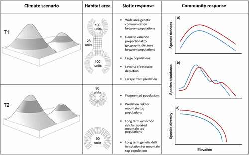
Today, alpine ecosystems are recognized as sensitive indicators of climate change (R. J. Wilson et al. Citation2005; Gobbi et al. Citation2007; Finch and Löffler Citation2009; Forister et al. Citation2010). Global temperature increase may force alpine communities to shift upslope, with increased susceptibility to fragmentation, stochastic events, and competition (). For example, Morueta-Holme et al. (Citation2015) repeated Humboldt’s Chimborazu measurements, showing a 500 m ascent of alpine communities during the preceding 207 years (2.4 m a−1).
Figure 1. The Diminishing Real Estate Model (DREM). The alpine biota (shaded band) undergoes two climate regimes. Upper left: At T1, cool adapted alpine biota occupy a broadly connected area of the mountain scape during cool climates. At T2, the climate has warmed, displacing and isolating the alpine habitat on separate peaks of the same mountain scape. The alpine habitats represent two frustums (conic sections) whose surface area can be calculated (center left column). Note that both frustum depths remain uniform while the radii reduce. Under the DREM, several ecological outcomes are possible across generation time (center right column). Within alpine habitats, community ecology indices are expected to have characteristic curves (colored lines) with increased elevation and, all things being equal, respond monotonically to climate warming (red) or cooling (blue). The model assumes typical species–area curves with the formula for a single mountain analogous to the island biogeography area curve: S= CAz, where S is the number of species, A is the area of frustum, and c and z are fitted intercepts
Although solar radiation and lapse rates differ between equatorial and temperate latitudes (Chen and Chen Citation2013), New Zealand alpine ecosystems may respond similarly to climate warming. Lacking approximately 210 years of data, information on New Zealand alpine ecosystems remains patchy (Macfarlane et al. Citation2010; Hoare et al. Citation2017). Climate and spatial data on alpine communities need to be acquired for ecological reference and for managing the alpine estate in a warming climate.
Here, we review the current understanding of New Zealand’s alpine invertebrate biota (AIB) in the Southern Alps () and present an investigation testing upslope tracking of that fauna. We couple population densities with elevation and relate these to a more than forty-year data set that indicates a constant rise of the end of summer snow line (EOSS).
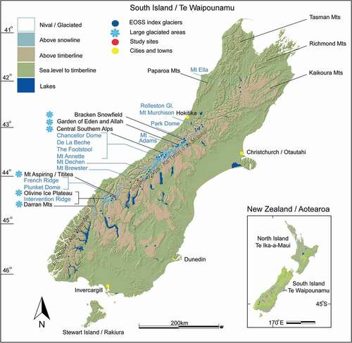
Figure 2. Map showing central Southern Alps of the South Island, Aotearoa/New Zealand, with additional mountain ranges labeled. Snow crystal icons show large regions of present-day glaciation. Dark blue dots are the end of summer snow line index glaciers (n = 50) including potential locations for establishing Climate Monitoring Units (CMUs), indicated in light blue. Brewster Glacier and French Ridge are marked in red
The Southern alps and its invertebrate biota
The South Island’s Southern Alps/Ka Tiritiri O Te Moana are New Zealand’s highest and longest mountain range, extending some 500 km (). Between 11 to 13 percent of the island is above the timberline (O’Donnell, Weston, and Monks Citation2017; this study), the majority of that includes the central alps, with Aoraki/Mt. Cook the highest point at 3,724 m a.s.l. We define the alpine zone as a spatial band extending from the climatic timberline to the permanent snow line (Wardle Citation1964; Burrows Citation1967; H. D. Wilson Citation1976; Mark and Dickinson Citation1997; Mark, Dickinson, and Hofstede Citation2000; Marris, Hawke, and Glenny Citation2019). Above the alpine zone is the nival, a composite of permanent snow, ice, and bare rock.
Most alpine-adapted invertebrates complete their life cycle between the timberline and permanent snow line. Populations about this zone are subject to the same climatic variables as most glaciers, including temperature (−15°C to +25°C), relative humidity (40–100 percent), precipitation (0–700 mm/h), radiation (short and longwave; 0.30–50 μm), insolation (e.g., 140 W/m2, direct and diffuse), wind (up to 180 kph), and air pressure (600–1,100 mb; N. J. Cullen and Conway Citation2015). In these conditions, invertebrates have shortened breeding, feeding, and developmental periods and usually overwinter under snow, avoiding predators and completing their life cycles (Sinclair, Lord, and Thompson Citation2001).
Many alpine invertebrates differ sufficiently from lower-elevation conspecifics to be considered separate species. These “true” alpine taxa share a suite of adaptive characters, notably, flightlessness, freeze physiology, melanism, omnivory, free-living life stages, hemimetaboly, dormancy, and sun basking or boundary layer retention behavior (Dillon, Frazier, and Dudley Citation2006). The orthoptera (weta and grasshoppers) represent alpine keystone species given their semimetabolous life cycle, physical mobility during all stages (except egg), omnivorous diet, freeze physiology, and diurnal activity (Field Citation2001) and as prey for alpine spiders (W. Chinn pers. obs.).
Climate change effects on the New Zealand alpine biota
Data from Antarctic ice cores, the Mauna Loa Observatory (Keeling curve), and New Zealand’s Baring Head Station show that CO2 levels have risen over a fifty-year period (Brailsford et al. Citation2012) and are far greater than any values recorded for the late Pleistocene (Etheridge et al. Citation1996; Lüthi et al. Citation2008). Carbon dioxide is a significant greenhouse gas and a major factor driving current atmospheric warming (Intergovernmental Panel on Climate Change Citation2014). Between 1950 and 2018 the concentration of CO2 rose from 300 to 412 ppm, a rate that is unlikely to cease within the next 100 years due to atmospheric inertia (C. D. Keeling and Whorf Citation2004; R. F. Keeling Citation2008; Sundquist and Keeling Citation2009). New Zealand’s average air temperature increased by 1.02°C between 1909 and 2017, a rate of 1°C per century and roughly one order of magnitude faster than the preceding 2000 years of global average (Mann and Jones Citation2003; Mullan et al. Citation2010; NIWA Citation2019a).
Between latitudes 40° and 50° S, the alpine biota experience persistent west-to-east circumpolar air currents, the so-called roaring forties (Pendlebury and Barnes-Koeghan Citation2007; Jiang, Griffiths, and Lorrey Citation2013; Strother et al. Citation2014). This climate regime maintains a four-way partitioning of humidity and temperature across the Southern Alps, specifically, warm + wet, warm + dry, cool + wet, and cool + dry. The effect has been correlated with speciation among alpine taxa (W. G. H. Chinn and Gemmell Citation2004; Heenan and McGlone Citation2012; Goldberg, Morgan-Richards, and Trewick Citation2015); however, the extent to which warming might alter this local climate scenario (and life history traits) remains unknown.
Alpine communities may respond to warming by (1) upslope habitat tracking, (2), in situ adaptation (via phenotypic plasticity or long-term selection), (3) horizontal migration, or (4) localized extinction of populations (). The upslope tracking model holds that populations will colonize higher substrates in lockstep with rising optimal (realized) niche parameters. We describe this scenario as the “diminishing real estate model” (DREM); see for a summary of effects.
Table 1. Potential responses of, and effects on, alpine invertebrate populations to a predicted rise in elevation of optimal habitat conditions, driven by a warming climate in the Southern Alps of New Zealand
The snow line as an ecological datum
Climate forcing of New Zealand’s alpine biota has an established theoretical pedigree (Cockayne Citation1928; Zotov Citation1938; Willet Citation1950; Fleming Citation1963; Bigelow Citation1967; Dumbleton Citation1969). These authors assumed that the entire alpine ecosystem will shift upslope (with warming) by slow colonization, relative to an ecological datum. By introducing the moniker “bio-glacial control,” Willet (Citation1950) established the fluctuating snow line paradigm. The snow line represents an isotherm with a hypothetical equator-to-pole thermal gradient (ETPTG), which clips the North Island volcanoes at 2,500 m, lowering to about 1,400 m in southern Fiordland, some 157 m/1° latitude (a 0.1° slope; Willet Citation1950).
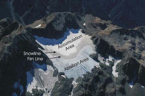
The EOSS is the highest net elevation of the regional snow line following cold-season snow accumulation and warm-season (summer and early autumn) melt (T. J. H. Chinn Citation1995; T. J. H. Chinn, Heydenrych, and Salinger Citation2005; Willsman, Chinn, and Macara Citation2015). Snow lines are influenced by precipitation, evaporation, temperature, albedo, and energy balance throughout the year. The EOSS is a transient feature and can be viewed on glaciers as dust-impregnated snow (firn) where seasonal snow accumulation equals loss (). Since 1978, an aerial photography program has documented the EOSS on fifty index glaciers (Willsman, Chinn, and Macara Citation2015). The snow line rarely, if ever, survives over bare rock (due to high-temperature radiative melting) and is necessarily measured on glaciers. In this capacity, the EOSS is important for approximating the equilibrium line altitude (ELA), a hypothetical elevation where glacier mass balance will be at equilibrium for a given location (Meier Citation1962; Nesje Citation1992). Currently, the Southern Alps EOSS is rising between 3.0 and 3.7 m a−1 and is correlated with climate warming (Willsman, Chinn, and Macara Citation2015; this study). Notably, snow line recession is seasonal and dynamic, whereas the EOSS rise is decadal (protracted) and significantly coupled to long-term response to ambient temperatures.
Figure 3. A typical End of Summer Snow line (EOSS) on the Rolleston Glacier, a very small cirque-type glacier in Arthur’s Pass National Park, Southern Alps. The glacier albedo acts to thermally buffer winter snow, which ablates slowly from the glacier snout at the onset of summer. The highest elevation of the snow line represents the average of all ablation sources and provides a relative position for the upper boundary isotherm of the alpine zone. Two snow patches are visible either side of the massif indicating that even under high Infra–Red radiation (from scree and rock) the snow line remains detectable
Multiple climate factors influence the EOSS in New Zealand. In a study by Purdie et al. (Citation2011), seven climate variables were correlated with snow ablation (water equivalent) on the Tasman Glacier and four were found to be statistically significant, including proximal sea surface temperature (0.579: p < .001), ambient air temperature (0.510: p < .001), the Southern Annular Mode (SAM; 0.344: p = .017), and the Southern Oscillation Index (SOI; 0.317: p = .026). The SAM represents a circumpolar ring of differential air pressure between the Antarctic and mid-latitude atmosphere and is closely linked to the SOI (Jiang, Griffiths, and Lorrey Citation2013). The EOSS may also fluctuate on decadal scales in response to latitudinal shifts of meridional airwaves, themselves a function of circumpolar troughs. Further climatological work by Mackintosh et al. (Citation2017) showed a connection between low- to high-latitude climate modes, regional atmospheric circulation patterns, sea surface temperatures offshore of the Southern Alps, and air temperatures, which collectively impact glacier mass balance.
The SOI measures atmospheric pressure differentials between Tahiti and Darwin, Australia (NIWA Citation2019c), and accounts for at least 30 percent of New Zealand’s seasonal climate variability as part of the El Niño–Southern Oscillation (ENSO) phenomenon (Troup Citation1965; Clare et al. Citation2002; Bhaskaran and Mullan Citation2003). For our purposes, the SOI typically manifests as weather pattern reversals (El Niño/La Niña seasons; ; Jiang, Griffiths, and Lorrey Citation2013). Because the SOI influences New Zealand weather by at least 25 percent (Purdie et al. Citation2011), we discuss the relationships between the SOI, the EOSS, and potential influences on alpine communities. It should be noted, however, that several modes of variability drive Southern Alps glacier response (Mackintosh et al. Citation2017), but for simplicity we evaluate New Zealand’s mid-latitude climate in response to tropical influences as represented by ENSO.
Table 2. Characteristics of the Southern Oscillation Index (SOI) and effects on New Zealand weather and snow line elevation in the Southern Alps
Testing the diminishing real estate model
Evidence supporting upslope tracking within the Southern Alps is limited (Halloy and Mark Citation2003; Harsch et al. Citation2009) and has met with some skepticism (McGlone et al. Citation2010; McGlone and Walker Citation2011). Studies relating timberline elevation with climate warming have also produced varying conclusions (Wardle Citation1985; Harsch et al. Citation2012). Beech forest seed production has been shown to increase with rising temperatures, although a considerable lag phase occurs (Wardle Citation1971, Citation2008; Whitehead, Leathwick, and Hobbs Citation1992). Efforts to detect the impact of atmospheric warming on alpine ecosystems include alpine grasshopper studies (White and Sedcole Citation1991; Koot Citation2018), timberline position (Wardle Citation1971; L. E. Cullen et al. Citation2001; Harsch et al. Citation2012; Case and Duncan Citation2014; Cieraad and McGlone Citation2014), plant community composition (Halloy and Mark Citation2003; Lord et al. Citation2017), and predator influxes (Christie et al. [Citation2017] and references therein).
Ensemble climate modeling has shown promise for relating geographic range shifts among New Zealand insects (Bulgarella et al. Citation2014), including alpine weta and grasshoppers (Sivyer et al. Citation2018). For example, Sivyer et al. (Citation2018) used MaxEnt (Elith et al. Citation2011) and other modeling approaches to suggest that mean annual temperature had the highest predictive power (>70 percent) for determining grasshopper range. Interestingly, they also found that isotherms had the lowest predictive power, yet our study relies on calculated isotherms in the alpine zone for population elevation. The EOSS, by contrast, is an actual elevation parameter, observable on the landscape. In all cases, correlating a warming atmosphere with a response by alpine communities requires at least two measures;
Multidecade climate trend data, specific to the alpine environment.
Biota physiologically coupled to the niche parameters within the alpine zone.
By coupling an appropriate environmental temperature lapse rate with a fixed elevation, we can expect the biota to experience warming at that location or to track upslope in order to maintain an optimal thermal envelope. For example, if the spring lapse rate at Mueller Hut in Aoraki/Mt. Cook National Park is about 6.6°C/1,000 m (Norton Citation1985), with a mean annual air temperature around 1.8°C at 1,760 m a.s.l. (NIWA Citation2019a, Citation2019b; Cliflo Citation2019), then we could expect an average temperature of 2.8°C in forty years, if scaled against the snow line rising at 3.7 m a−1. The question is does the alpine biota adapt or shift in step with this rate function?
Conservation and alpine populations
The goal of alpine conservation is maintaining range, diversity, and pattern of high-elevation indigenous communities. The impact of climate warming on New Zealand’s alpine diversity remains unclear despite high endemism (up to 90 percent), with populations confined to single mountain ranges (W. G. H. Chinn and Gemmell Citation2004; Mark Citation2012). Greater predictability of climate effects would assist management while providing an ecological “early warning.” Ideally, alpine climate models should calculate extinction risk for select populations using three terms: which mountainous regions will be most affected (spatial), when climate warming effects might manifest (temporal), and at what rate alpine communities might respond (a constant).
Habitat area is an important consideration for extinction risk (Rosenzweig Citation1995). Rapid climate warming may fragment invertebrate populations, leading to critically small sizes. On the other hand, long-term (>1,000 years) segregation can drive speciation through genetic drift in isolation (Trewick Citation2001, Citation2005; Buckley and Simon Citation2007; Trewick and Morgan-Richards Citation2019; Trewick, Wallis, and Morgan-Richards Citation2011; Wallis et al. Citation2016), the so-called Pleistocene species pump (Schoville, Roderick, and Kavanaugh Citation2012). Assessing long-term persistence will involve a trade-off between the rate and extent of environmental change and the adaptive capacity of populations. Community-level indices of the alpine biota are critical because species richness is expected to decline as the climate warms (Peters Citation1992; Schneider Citation1992; Parmesan Citation2005). However, species abundance is less clear because the biomass of a keystone species may increase at specific elevations ().
Current management of New Zealand alpine ecosystems includes bird and lizard monitoring, specifically Rock Wren (Xenicus gilviventris) and Kea (Nestor notabilis), and to some extent alpine gecko (O’Donnell, Weston, and Monks Citation2017). This work is framed within ecological management units (EMUs), areas in which community indices are repeatedly measured. The Southern Alps are conveniently scaled for EMU work. Cirque basins, long valleys, and spurs offer useful ecological gradients. Table mountains and sharp climatic gradients present natural limits to populations which can be employed to protect and monitor communities. The Zero Invasive Predators (ZIP Citation2018) initiative in the Perth Valley, west of the Main Divide is an example. We propose augmenting alpine EMUs with climate monitoring units (CMUs), potentially stimulating an alpine climate and conservation paradigm.
Aims
We investigate three themes: (1) Can upslope tracking be detected using the EOSS as a climate proxy? (2) What rates of upslope movement can we estimate using alpine invertebrates? (3) An assessment of the alpine invertebrate fauna for monitoring climate change effects on alpine ecosystems.
Methods
Study sites
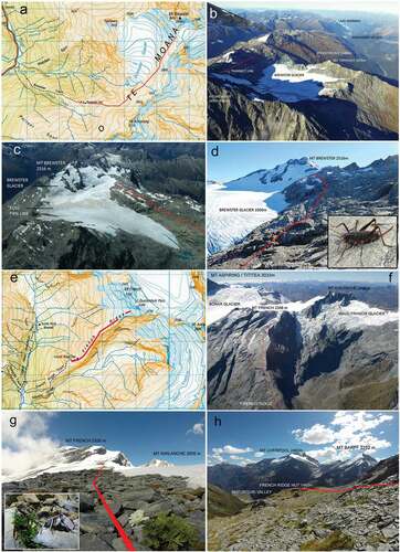
We selected two alpine study sites Brewster Glacier (44°4′15″ S, 169°26′11″ E) and French Ridge (44°25′20″ S, 168°42′09″ E; , -h). Brewster Glacier is a significant glaciology and climatology research area (George Citation2005; Willis et al. Citation2009; Anderson et al. Citation2010; Gillet and Cullen Citation2011; N. J. Cullen and Conway Citation2015; N. J. Cullen et al. Citation2016; Sirguey et al. Citation2016), and data from those studies may benefit future ecological work. French Ridge, located in Mt. Aspiring/Tititea National Park, is 70 km southwest of Brewster Glacier and represents an ecologically confined ridge system. French Ridge is situated between two EOSS index glaciers (Fog and Findlay; 14 and 23 km, respectively).
Figure 4. Composite images of the two sampling locations, Brewster Glacier (a-d) and French Ridge (e-h). Both sites support an ecologically isolated biota, confined to a ridge and extending from the timberline to the permanent snowline (or mountain summit). (a) Map of the Brewster Glacier and environs (Topomap 1:50 000 Series). Red line depicts invertebrate sampling transect, grid squares=1km. (b) aerial photograph of Brewster Glacier in 2016, view toward south west. (c) Typical snowline aerial photograph of Brewster Glacier showing firn line and End Of Summer Snow line (EOSS) with sampling transect (red line). (d) Ground view of Mt Brewster taken from transect line. Image insert is a female Pharmacus brewsterensis: Rhaphidophoridae, a resident of this habitat. (e) Map of French Ridge, Mt Aspiring/Tititea National Park (Topomap 1:50 000 Series). Red line depicts invertebrate sampling transect. Grid squares=1km. (f) Aerial photograph of French Ridge (showing transect) and Bonar Glacier. (g) View looking up to Mt French, from 1800 m a.s.l. Tapering red line represents transect path. Insert image shows the scree weta Deinacrida connectens feeding (at night) on a native Ranunculus herb. (h) Down-slope view of French Ridge showing hut location, sampling transect and example of alpine herb field/stone pavement
Invertebrate sampling
Invertebrates were sampled from transects between 1,400 and 2,200 m a.s.l. (800 m vertical, the maximum range for thermal effect). Sampling occurred in March 2016 (the last month of highest snow line in the Southern Alps) and coincided with the EOSS survey flights.
At 100-m contours, quadrat lines (N = 9) were established perpendicular to the main transect with five quadrats per line. Quadrats were 3 × 3 m with 15-m separation over 60 m. If terrain or obstacles prevented a complete line, the series was extended in the opposite direction. Invertebrates were counted per hour, per 100-m contour, and the highest density per elevation (the median) was used to infer the optimal thermal niche. Two people made counts by eye. Raw data were collected with counters and score cards, and elevation and distance were determined using a Garmin 62s Global Positioning System instrument and tape measures.
Invertebrate collecting was by hand, sweep net, and rock turning (day and dusk). Timed sweep netting of vegetation was employed for flying insects. Specimens were identified to species or lowest recognizable taxonomic unit. We omitted diptera from the study, a diverse group difficult to correlate with elevation. Representative specimens were preserved and lodged with the author’s collection at the Department of Conservation.
Population densities
Population density × Elevation was assessed using the violin plot function in R Studio and ggplot (R Core Team Citation2013). For these plots, invertebrate counts per contour were normalized against the highest value in order to visually accommodate the range (without resorting to a log scale or similar). Significance tests were performed in R (R Core Team Citation2013; Richards Citation1972).
The EOSS data set as a climate proxy
Long-term climate trend data are required to correlate alpine community responses to change.
In New Zealand, long-term in situ observations above 1,000 m are sparse (fewer than fifteen climate stations) and temporally incomplete, hindering ecological study. The EOSS survey provides surrogate long-term environmental data on the alpine zone with inherent linkages to multiple climate variables, particularly temperature.
Snow line elevations were derived from aerial photographs of fifty index glaciers (). The photographic series began in 1978 and continues today (Willsman, Chinn, and Macara Citation2015; SIRG Citation2019). Prior to the 1990s, the EOSS was estimated from photographs by eye, a method that incurred unknown error. Since 2001, the photographs were orthorectified in Photogeoref v 1.0 (Corripio Citation2004) using five correction variables: camera Global Positioning System position, focal length, image size, land digital elevation models, and ground control points (cross-referenced with topographical maps).
Table 3. Summary data for fifty snow line index glaciers in the Southern Alps, New Zealand. Glaciers are listed geographically from north to south
Snow line elevations are derived values, estimated from plotting an expert guided snow line demarcation against a geodetic topographic map. Following digitization of the glacier snow lines, an ablation-to-accumulation ratio is calculated. Snow line elevations can then be accurately assessed from an area–altitude curve for each glacier or directly from a digital elevation model (Willsman, Chinn, and Macara Citation2015, Citation2017). These values were used for our analysis.
Snow line trend data
Snow line elevations were plotted (linear regression) against space and time to assess slope and trend throughout the Southern Alps. Linear distance was measured on longitude with the Kaikoura Mountains as a datum for all plots. Rates of annual snow line rise were derived by the equation (slope × T2 + intercept) − (slope × T1 + intercept). The relationship between the snow line and timber line was also investigated. Timberline elevations were derived from 1:50,000 scale maps (NZ Topo50 Series) within a 5-km orbit of index glaciers. Where visible, timberline elevations were cross-referenced with aerial photographs per glacier.
Southern oscillation index
Frequency and amplitude of the SOI were assessed as a composite of snow line elevation and, by association, invertebrate population elevation. The SOI was selected as an index to explain snow line fluctuation because it convolves several atmospheric and surface climate variables and has a strong relationship with Tasman sea surface temperatures, which in turn correlate strongly with glacier volumes and the ELA (Purdie et al. [Citation2011]; Bowen et al. [Citation2017] and references therein; Mackintosh et al. [Citation2017]). The SOI was acquired from the U.S. National Oceanic and Atmospheric Administration and constrained for the period 1977 to 2016 prior to correlating and plotting annual snow line data (NOAA Citation2019).
The snow line tracking model
Our model () includes five assumptions: (1) Population densities are thermally coupled to elevation. (2) Population densities have remained thermally linked to elevation for the preceding forty years (the snow line data period). (3) Upslope movement is proportion to shifts of the snow line isotherm between periods T1 and T2. (4) For a given slope, the elevation differential between the snow line at T2 and population median provides a rough colonization rate (m a−1). (5) If all populations are strictly coupled to the snow line elevation, we should expect faster rates of colonization across shallow slopes compared to steep slopes (varying rates for equivalent vertical gain and period). Conversely, if elevation varies across differing gradients following an equal time period, then abiotic isotherm tracking may be subordinate to biotic factors.
Figure 5. Model of upslope habitat tracking by an Alpine Invertebrate Biota (AIB). Colored temperature ellipses represent populations of different species and their optimal (realized) niche elevation. Densities are represented by three median width classes. The diagram shows an upslope shift of 120 m by the End of Summer Snow line (EOSS) between 1977 (T1) and 2017 (T2), a response correlated with atmospheric warming. T2 populations located at, near, or even extending into the previous snow line are assumed to have tracked up slope since T1. Populations can be directly sampled today for occupancy on snow- and ice-free slopes at T2. Nine populations protrude above the T1 snow line (blue dashes). For the remaining populations, upslope tracking has occurred if their T2 median densities are at elevations previously cooler than today’s apparent optimal temperatures, given a lapse rate of 6.6°C km−1 relative to the snow line. The “red” population provides an example; at T2 the highest population density is located at 1,520 m a.s.l., with an isotherm of 3.6°C. Forty years ago, the same isotherm was 120 m lower
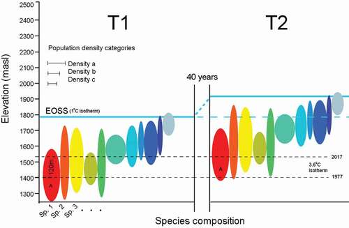
The model includes an estimate of the snow line isotherm. We derived an average snow line elevation for the Southern Alps at 1,600 m a.s.l. (excluding the ETPTG) across all years by converting the glacier ELA to meters above sea level using data from Willsman, Chinn, and Macara (Citation2015, Citation2017). At 1,600 m a.s.l. the snow line isotherm was calculated using an eighty-year temperature record from near sea level (at Hokitika airport, Westland; NIWA Citation2019d). Coupling the mean sea level temperature at Hokitika (11.5°C) with a 6.6°C km−1 lapse rate gives an estimated mean annual temperature of 0.94°C for the snow line, our isotherm of interest. Detailed studies of environmental lapse rates in New Zealand are limited, and we have not included the various uncertainties here. The 6.6°C km−1 lapse rate conforms to Norton’s alpine spring maximum (Norton Citation1985; Tait and Macara Citation2014) and serves to test the fidelity of alpine invertebrate communities to narrow thermal zones since a high lapse rate may amplify any tracking signal (EquationEquation (1)(1)
(1) ):
Hokitika is situated near the Southern Alps (42° S and 33 km from the main divide), approximately halfway along the Alps. A measurable shift of the snow line represents a repositioning of the 1°C isotherm and potential ecosystem driver. Populations of the AIB located adjacent to the EOSS should track at a rate equal (or similar) to the snow line shift (EquationEquation (2)(2)
(2) ):
where AIBer indicates alpine invertebrate biota elevation rise, ΔSl is the change in elevation of the snow line, and Δyr is the number of years elapsed between snow line elevations.
For populations below the snow line, maximum densities are assumed to be static at specific elevations, whereas isotherms shift upslope with warming. Alternatively, those populations may keep pace with their optimal thermal envelope; that is, track. Because we cannot go back in time to observe shifts, we can measure the relative density of today’s population elevation and construct density elevation plots. Then we calculate the optimal isotherm (and elevation) for maximum population densities (EquationEquation (3)(3)
(3) ):
where Opop is the observed population elevation, PopT is the optimal temperature of population at T2, ∆TSL is the temperature change of snow line rise, and oC km−1 is the lapse rate (6.6°C/1,000 m).
Expanding the above equation terms gives
PopT = (Δ elevationSL-CP) × (Lapse rate) + TempSL,
where Δ elevationSL-CP is the elevation difference between T2 snow line and T2 population elevation, the lapse rate = 6.6°C/km−1, TempSL = + 1°C, CP is the core population elevation, SL is the snow line elevation, and
∆TSL = (T2 snow line elevation − T1 snow line elevation) × (6.6°C/km−1).
Slope geometry
Snow lines and alpine communities represent positions on the hypotenuse of a right angle triangle (the mountainside). For an equivalent vertical movement, elevation shifts will appear faster on shallow slopes relative to steep slopes. We can exploit this property to roughly differentiate between biotic and abiotic drivers of elevation change. For example, if the AIB is coupled to an isotherm, a shift of that optimum should induce varying rates of colonization depending on the slope gradient. Conversely, if upslope colonization does not change across varying slopes, irrespective of an upward shift of the snow line (isotherm), biotic or other factors may be more significant than maintenance of a given thermal zone.
Under this scenario, population-level adaptation may be occurring, expressed as behavioral and physiological plasticity; for example, locating mates, predator avoidance, reduced competition (inter and intra), or exploiting an increase of organic matter as the snow line rises. In all cases, it will be necessary to calibrate tracking rates at each location as part of any model seeking to measure elevation change of the biota. The goal would be to plot varying rates of population shift throughout the Alps, highlighting regions with “slow” or “fast” tracking rates, if indeed they occur.
Climate monitoring units
We made a desktop assessment of locations within the Southern Alps suitable for establishing CMUs. Criteria included ecological isolation, contiguous habitat from subalpine to nival, conical mountains, cirques or broad ridges extending from valley floor to mountaintop, and close proximity to index glaciers with measurable snow lines (details in ).
Table 4. Site selection criteria for establishing Climate Monitoring Units (CMUs) and measuring upslope tracking of the End of Summer Snow line (EOSS) by alpine invertebrates in the Southern Alps of New Zealand
Results
The alpine invertebrate biota
Slope and total recognizable taxonomic unit counts for Brewster Glacier and French Ridge were respectively 11° and twenty-nine and 20° and twenty-five (see for species checklist). Species abundance and richness curves were typical: few groups with numerous individuals and many taxa with few ( and ). Taxon richness at Brewster Glacier showed a negative relationship with elevation, where the highest proportion of taxa was at 1,600 m a.s.l. (R2 = 0.965), between shrublands and alpine snowgrass. Values were derived from a best-fit, least-squares fourth-order polynomial (). Results from French Ridge also showed a negative richness relationship with elevation (linear best-fit model R2 = 0.946; and ).
Table 5. Checklist of alpine invertebrate taxa from Brewster Glacier and French Ridge, considered as members of the Alpine Invertebrate Biota (AIB). Maximum counts per elevation (at T2) are listed
Figure 6. Alpine invertebrate species abundance plots for (a) Brewster Glacier (n = 29) and (b) French Ridge (n = 25). Data are total individual counts per taxon; elevation range was from 1,400 to 2,200 m a.s.l. Both locations generated characteristic curves, with few taxa represented by many individuals and many with few counts. Grasshoppers represent the majority of alpine invertebrate biomass, probably reflecting the density of snow tussock (Chionochloa sp.)
Figure 7. Species richness curves (number of taxa) per 100-m contour for (a) Brewster Glacier and (b) French Ridge. Both locations show strong negative trends. For Brewster Glacier, a fourth-order polynomial curve provided the best fit (R2 = 0.965). Taxon richness peaked at around 1,600 m a.s.l., declining by approximately five taxa per 100-m upslope shift. For French Ridge the best-fit trace was linear, with a strong negative trend (R2 = 0.947). French Ridge taxon richness declined at 2.7 taxa per 100 m of elevation gain
Grasshoppers (Sigaus australis) were 30 percent more abundant at Brewster Glacier (n = 426; 1,400 m a.s.l.) than cockroaches, the next highest taxon group (n = 129). Grasshopper median density declined to less than five insects per hour by 1,900 m a.s.l. Conversely, cave weta (Pharmacus chapmanae), first appeared at 1,700 m a.s.l. (n = 6) and at 1,900 m a.s.l. the conspecific P. brewsterensis was detected (at two per hour). By 2,100 m a.s.l., P. chapmanae counts were highest for any taxon at that elevation (twenty-eight per hour). At Brewster Glacier species richness declined to six taxa by 2,100 m a.s.l., including cave weta (P. chapmanae and P. brewsterensis), a terrestrial micro snail (Charopidae), alpine cicada (Maoricicada sp.), soil centipedes (Geophilomorpha), and the mountain ringlet butterfly Percnodaimon merula.
At French Ridge Sigaus australis grasshoppers were less abundant (109 versus 426 at Brewster Glacier) and land hoppers (Talorchestia sp.) were common (forty-eight per hour at 1,400 m a.s.l., declining to one specimen at 1,600 m a.s.l.). Snow grass (Chionochloa sp.) is a major forb for alpine grasshoppers, and French Ridge supports considerably fewer than the Brewster Glacier environment. Punctid snails were most frequent at 1,400 m a.s.l. (n = 14/h) and at both locations snails were found within crevices, moss clumps, and short-stature herbs (Ranunculus sp.). Both sites showed a consistent decline in diversity and richness with increasing elevation. Taxa above 1,700 m a.s.l. became restricted to a high-altitude assemblage of moss beetles (Byrrhidae), cave weta (Rhaphidophoridae), mountain ringlets (Percnodaimon), spiders (Lycosidae and Salticidae), cicada, and snails (Punctoidea). Of cicada, four individuals were detected per hour at 2,200 m a.s.l. up to the snow line.
Population density and elevation
Elevation data are presented in and . Most invertebrates were between 1,400 and 2,000 m a.s.l., although three taxa at Brewster Glacier were present at 2,200 m a.s.l., higher than the local EOSS. Values for lower elevation taxa are likely to overestimate the median elevation because counts were not taken below 1,400 m a.s.l. (the minimum sampling elevation). Several medians clustered at the same elevation, a potential sampling bias.
Figure 8. Violin plots showing relative densities of invertebrate populations for T2 (March 2016) at (a) Brewster Glacier and (b) French Ridge. Black dots are population medians; horizontal blue lines are snow lines (T1 and T2). Any taxa extending above the snow line were present either on snow or basking on rock outcrops close to the 2016 snow line. Colors are representative of woody shrubland (green), snowgrass (beige), and rock/snow (blue). Above 1,800 m a.s.l. the alpine habitat comprised short-horned grasshoppers (Acrididae), cave weta (Rhaphidophoridae), and free-living alpine wolf spiders (Anoteropsis alpina)
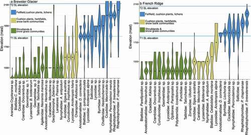
At Brewster Glacier, 55 percent of taxa were classifiable as members of the AIB (i.e., their vertical distributions were confined by lower and upper boundaries). At French Ridge, 60 percent were classifiable alpine species (including populations with a distribution “taper”; ). The remaining taxa show density tails extending below 1,400 m a.s.l., indicating a wide elevation range. For example, the ubiquitous New Zealand wolf spider Anoteropsis hilaris was sampled between 1,400 and 1,900 m a.s.l. despite being known from sea level to the alpine zone.
At least 72 percent of high-elevation taxa were shared between locations with cave weta (P. chapmanae and P. brewsterensis; Rhaphidorphoridae), the highest at both sites (from 1,600 to 2,200 m a.s.l. and higher). These weta species are among the highest free-living, flightless insects in New Zealand.
Snow line spatial trend
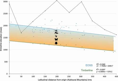
Summary data for the fifty index glaciers are provided in . For the years 1977 and 2016, the mean rate of snow line rise was 3.73 m a−1 (SD = 1.8), with an acceptable difference of 0.7 m. The regression fit of all snow line data (n = 3,207) against latitude (linear distance) shows a 0.07° slope, approximately 130 m per degree of latitude (). The timberline showed a consistent 800-m separation below the snow line, the intervening area representing the alpine zone. We interpret the total slope as the Southern Alps ETPTG.
Figure 9. Graph showing elevations for the end of summer snow line (upper blue line) and timberline (lower green) plotted against latitudinal distance from the Kaikoura Mountains to Fiordland. Data are from fifty index glaciers in the Southern Alps of New Zealand and monitored between 1977 and 2016. Timberlines derived from 1:50,000 topographic maps. The snow line and timberline descend at approximately 130 m per degree of latitude (data from Willsman, Chinn, and Macara Citation2015, Citation2017). Colored shading represents our definition of the alpine zone and the region inhabited by the Alpine Invertebrate Biota (AIB), indicated as invertebrate silhouettes. Skyline trace shows high point elevations of mountains at specific distances from origin
Snow line temporal trend
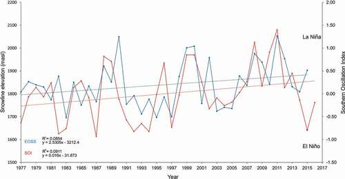
shows the total snow line (and SOI) data for all index glaciers from 1977 to 2016. The small positive correlation (0.144) was significant, t(3192) = 26.6057, p = .001, α = .05, x̄ = 1,841.4 (m a.s.l.), n = 1,597, σ = 235.28, σx̄ = 5.894. Slope calculations indicate a snow line rise of between 3 and 3.7 m a−1 across all index glaciers. Data points are considerably scattered about the regression line although up to 85 percent of the error is a function of the index glacier latitude relative to the ETPTG slope. Snow line elevation data oscillated about the mean by 55 m a−1 (σ = 27.8; n = 23). Eight seasons showed oscillations greater than 100 m at an average frequency of five years (σ = 3; blue line); a local climate response to regional conditions arising from the Southern Oscillation (red line; see below).
Figure 10. Combination graph showing a relationship between actual End of Summer Snow line (EOSS) data (blue line) and the Southern Oscillation Index (SOI), sea level air pressure anomaly as fluctuating red line. The ascending linear blue line traces the least-squares fit for the EOSS data. The red line trace shows an increase of the SOI over the same period. Here, the snow line rises at 3.10 m a−1 with a 0.144 correlation coeffcient (significantly greater than zero). The EOSS was correlated with SOI fluctuations (Kolmogorov-Smirnov test: D = 0.5, p = 0.1678). Positive SOI values represent La Niña weather anomalies and negative values represent the El Niño system
Snow line trend for Brewster Glacier and French Ridge
Site snow line tends are shown in and . Brewster Glacier indicated a snow line rise of 5.73 m a−1 between 1978 (1,800 m a.s.l.) and 2016 (2,010 m a.s.l.; R2 = 0.1573). The Findlay Glacier snow line (French Ridge proxy) showed a 4.45 m a−1 rise over thirty-four years (130 m; R2 = 0.1531). This 29 percent difference between Brewster Glacier and Findlay Glacier illustrates the local variability of the snow line isotherm and the potential sensitivity of the alpine biota to localized mountain ranges.
Figure 11. Local End of Summer Snowline (EOSS) plots for each sampling site. Upper plot: Snowline rise for Brewster Glacier showing a rate of 5.73m a-1 (y5.7438x -9549.8 = 2023m–1811m a-38). The positive correlation (0.43) was significant: t(34) = 22.2715, p < 0.05, x̄ = 1923, σ = 157.88 (R2 = 0.16). Lower plot: Snowline rise over 35 years for the Findlay Glacier (nearest analogue to French Ridge) showing a rate of 4.45m a-1, between years 1981 and 2016. The positive correlation (0.40) was significant: t(32)=22.2715, p < 0.05, x̄ = 1690, σ = 101.82 (R2 = 0.1531)
Southern Oscillation Index
Correlating the SOI and the EOSS data produced a slightly significant but ambiguous positive coefficient (0.520), t(2) = −116.8, p = .05 (). Additional analysis using a nonparametric Kolmogorov-Smirnov test was significant, D(20) = 0.5, p = .1678 (i.e., the data were from the same distribution with no overall difference in shape).
illustrates the phase relationship between snow lines and the SOI. which peaks at a one- to two-year lead on the EOSS. Several features of the SOI plot are noteworthy: (a) over half of the SOI accounts for the EOSS variability per year; (b) amplitudes of the EOSS oscillations are tightly coupled to the four highest SOI positive values for the years 1989, 1999, 2007, and 2011 (ten, eight, and four years, respectively), but the reverse was not true; and (c) a positive SOI appears the greater driver of upslope snow line elevation (than negative values for lowering the snow line).
Positive SOI values are representative of the La Niña (warmer) air mass systems (anticyclones from the north) and lower snowfall. However, the year 2015 shows a decoupling between the negative SOI (−0.7500) and EOSS (1,900 m a.s.l.). In both cases, there was a positive trend (R2 = 0.09 and 0.08).
Snow line tracking: Actual
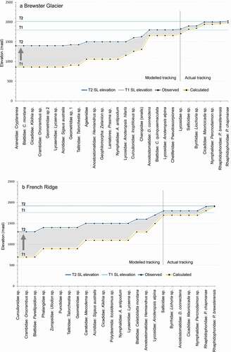
In and we present a synthesis of our model. The plots combine the EOSS, the AIB, two time periods, and both sites. The graphs show upslope shifts of several invertebrate populations from the T1 snow line elevation. The weta Pharmacus brewsterensis and P. chapmanae tracked at a rate equivalent to, or greater than, the maximum snow line rise at both sites (5.73 m a−1 at Brewster Glacier and 4.45 m a−1 for Findlay Glacier/French Ridge). This indicates that the weta are nearly equivalent in colonization ability at each site.
Figure 12. A synthesis of the model. Each graph shows four variables: The End of Summer Snow line (EOSS), the Alpine Invertebrate Biota (AIB, on abscissa), two time periods, and the two sites (a) Brewster Glacier and (b) French Ridge. Blue and yellow lines represent observed and calculated population density–elevation values, respectively. Snow line elevations are shown by the two horizontal blue lines for T1 and T2. For Brewster Glacier the snow line has risen 220 m, with seven taxa occupying slopes previously under the end of summer snow line some thirty-eight years ago (actual tracking). Six of those taxa had medians located at 1,800 m a.s.l. and two were measured at about the T2 snowline (1,910 m a.s.l.). This suggests that those taxa have actively tracked the snow line but not necessarily at the same rate. By contrast, the modelled tracking rise shows a considerably greater increase (up to 600 m) in elevation of populations over the same time period. The French Ridge (Findlay Glacier) snow line elevation shift was 160 m between T1 and T2. Lower elevation taxa potentially shift further with a rising snow line, whereas high elevation taxa are confined to a narrow thermal zone. The area between the taxa elevations is suggestive of a hysteresis function. See Discussion for details
By contrast, several taxa presented slower tracking rates. At Brewster Glacier, the median for jumping spider and moss beetle populations was 1,900 m a.s.l., midway between the T1 and T2 snow line elevations, with a nominal upslope tracking rate of at least 2.7 m a−1. At French Ridge, five taxa were detected midway between T1 and T2 snow lines, some 40 m above the (proxy) T1 snow line, indicating a tracking rate of 1 m a−1. The French Ridge taxa comprised jumping spiders, moss beetles, weta (Deinacrida connectens), Maoricicada, and mountain ringlets (Percnodaimon sp.).
Evidence of long-term invertebrate presence at elevations previously above the snow line (for at least thirty years) included silken retreats, exoskeleton molts, frass accumulation, and abandoned occupancy cells showing persistent mechanical redistribution of particulates. Taxa of particular interest included moss beetles (Liochoria sp.: Byrrhidae), jumping spiders (Salticidae), and two weta groups—the scree weta Deinacrida connectens and the cave weta P. brewsterensis and P. chapmanae—at both sites. These high-elevation taxa have limited dispersal ability (most are flightless) and nearly all are detritivores or scavengers, except for the spiders, which presumably feed on weta, collembola (spring tails), mites, and possibly pscoids (Psocoptera).
Snow line tracking: Modeled
The model formula was applied to all T2 median values (actual elevations). Populations at lower elevation showed greater apparent vertical movement than those at higher elevation, particularly for populations at 1,400 and 1,500 m a.s.l., in contrast to those at higher elevations (1,600–2,000 m a.s.l.; and ).
At Brewster Glacier there was an apparent difference of 543 m between actual and calculated population elevation for seven taxa (the landhoppers, day flying moths, spiders, cockroaches, weevils, grasshoppers, and grass cicada). The elevation differential reduced to 518 m (for Geometrid moths), 443 m for Agelenid spiders, 143 m for D. connectens weta, and as little as 43 m for P. chapmanae. French Ridge data showed a similar taper in elevation differential between T1 and T2, specifically 603 m (weevils), 403 m (Mecodema ground beetle), 303 m (cockroaches), 63 m (jumping spiders), and 0 m for P. brewsterensis. The maximum calculated upslope tracking rates for lower elevation populations was about 16 m a−1, at least five times greater than that for the snow line taxa.
For taxa occupying elevations above 1,700 m a.s.l., their summer average was probably close to 0°C (and cooler during winter). Those taxa were apparently restricted by the 1°C isotherm (snow line), with smaller shifts within the temperature/elevation envelope, in contrast to lower populations. These “confined taxa” included the weta (D. connectens, B. brewsterensis, and P. chapmanae), spiders (A. alpina, Lycosidae, and jumping spiders) and Maoricicada sp., byrrhid beetles, and the mountain ringlet Percnodaimon sp.
Nevertheless, populations showed a time-dependent rising trend relative to the snow line rise. Although the snow line positions are stepped (220 m for Brewster Glacier and 160 m for Findlay Glacier), the invertebrate populations show a convergence between actual and calculated elevation, per unit of height gain.
Climate monitoring units
We selected fifteen candidate locations in the Southern Alps meeting our criteria for long-term CMUs (, ). Each site included (or was close to) an index glacier where the recorded snow line rise was at least 2.0 m a−1. Most sites were sufficiently high for the snow line to encompass at least 70 percent of a mountain’s circumference, which is desirable for testing the DREM.
Table 6. List of Southern Alps locations with potential for establishing Climate Monitoring Units (CMUs). Each location has a corresponding index glacier (within 8 km of the monitoring site), which can provide End of Summer Snow line (EOSS) elevation data
Several sites fell within the Southern Alps “beech gap” (Orwin Citation2007) and others were within beech-forested mountains (). This geographic spread presents an opportunity to test beech and non-beech ecosystems under the same climate shifts. In our opinion, alpine invertebrates offer multiple advantages for investigating ecological responses to climate shifts. Consequently, we provide a list of candidate invertebrate taxa and their ecological information ( and ). These taxa are common to the Southern Alps and are generally confined to subalpine and alpine zones. We assume that these taxa are responding to optimal niche parameters including life cycles that use all, or part, of the available substrate (Nagy and Grabherr Citation2009).
Table 7. Candidate invertebrate taxa for monitoring alpine ecosystem condition within Ecological Management Units (EMUs) and Climate Monitoring Units (CMUs). Taxa are common to the New Zealand Southern Alps
Discussion
The snow line monitoring program shows a dramatic reduction of ice volume throughout New Zealand’s mountain glaciers (T. J. H. Chinn et al. 2012; Mackintosh et al. Citation2017; NIWA Citation2020). As time elapses, the data set becomes increasingly reliable, and today the study represents one of the longest proxy climate records from within the Southern Alps. In this article, we have explored the ecological utility of the snow line data as a complementary measure of climate forcing on alpine communities (Willet Citation1950; Fleming Citation1963; Wardle Citation1971; Burrows Citation1990; Mark Citation2012).
During the 1990s, the climate control paradigm saw renewed interest as DNA sequencing tools provided fresh estimates of population divergence times, particularly when coupled with molecular genetic clocks (Avise Citation2000). When applied to New Zealand’s alpine invertebrates and plants, genetic analysis has shown that long-term habitat tracking has been the rule, especially during the Pleistocene and early Holocene climate fluctuations (Gibbs Citation1999, Citation2016). However, few studies have provided rate functions for these elevation shifts, despite this being a necessary prerequisite for the tracking model to hold. More pressing is today’s current rate of warming (at least 1°C per century), driving an unprecedented rise of the snow line (by at least 3.7 m a−1). At this rate, the potential to force alpine populations into local extinction under the DREM is considerable if habitat tracking holds true.
Did we answer our questions?
Our study showed that all taxa above 1,800 m a.s.l. had indeed tracked upslope in the preceding thirty-eight years of snow line rise ( and ). Below 1,800 m a.s.l. tracking results were calculated values only, and there was considerable rate variation, which is open to interpretation. Small groups of high-elevation taxa (cave weta in particular) tracked within a narrow isotherm band (or at least colonized refugia recently exposed). For these taxa, measured tracking rates were at least as fast as the upslope shift of the snow line (approximately 3 m a−1). Meanwhile, at lower elevations the calculated shift rates appeared larger, showing higher vertical differentials with a maximum upslope rate around 16 m a−1, shown in and as a time-dependant convergence between actual and calculated taxon elevations. We interpret the shape of these graphs as hysteresis curves, also known as “alternative state theory” (Lewontin Citation1969).
In our opinion, the convergence situation describes an ecological lag function (a hysteresis; Doering et al. Citation2007; Bader, Rietkerk, and Bregt Citation2018). Although speculative, we suggest that lower elevation populations have a wider thermal tolerance than those at higher elevations (near the snow line). In our case, the area between the actual and calculated population (median densities) indicates “work done” (Vertical movement × Number of taxa) by the entire community at specific elevations. The degree of population lag (the graphed area between past and present) apparently depends on the rate and extent of the vertical shift for a given isotherm. Comparing population trends between sites is perhaps best interpreted using integrals for the two time curves (T1 and T2), per site; for example,
We estimate that the alpine hysteresis curve will persist as the snow line continues to rise. With further warming, the area of the curve may become deep and wide as more taxa (including introduced) are able to make a greater elevation shift between any given T1 and T2 position. On that basis, alpine ecosystems may never return to the same population-elevation configuration as they were at T1 even in the unlikely event that temperatures were to again cool in the next few centuries.
The Southern Oscillation and CMUs
Our analysis showed a relationship between the SOI and EOSS elevation, consistent with the findings of Purdie et al. (Citation2011) and Salinger, Fitzharris, and Chinn (Citation2019). In these studies, ENSO-driven temperature was a stronger influence on snow line elevation than precipitation (Mackintosh et al. Citation2017). Although we are aware of the very close relationship between temperature and ice volume change in the Southern Alps, other modes of climate variability also exert significant influence on regional temperature patterns (Mackintosh et al. Citation2017). Therefore, we caution reliance on the SOI for anything other than investigating ecological oscillations in the alpine habitat and broader climate studies.
When combined with several regional climate indices, the SOI will be an important part of EMU and CMU data. For instance, during El Niño (negative SAM) conditions, alpine invertebrate communities may be depressed into lower elevations and potentially more prone to rodent predation. The reverse is true for La Niña years (positive SAM), because warmer temperatures and less precipitation favor a snow line rise (and a vertical “stretching” of the alpine zone). In all cases, it is advection of temperatures onto New Zealand from several thousand kilometers that appears to be the most important factor controlling Southern Alps air temperatures (Mackintosh et al. Citation2017). In this light, even during cool years (El Niño), Tasman Sea temperatures may be warmer than normal.
During the austral summer of 2017–2018, New Zealand experienced an unprecedented marine and atmospheric heat wave. The regional heating covered about 4 million km2, with air temperatures across New Zealand higher than any recorded in over a century (BoM and NIWA Citation2018). A consequence of this warming saw the highest snow line elevation since records began (T. J. H. Chinn, pers. obs.). This illustrates the impact of extreme temperature swings in the alpine environment and highlights the urgency to establish baseline ecosystem information from a series of CMUs. We suggest that alpine CMUs should measure a suite of climate variables in conjunction with population elevations. Because we do not yet know the critical area and density values that may herald imminent population extinction we should, at least, establish a datum and monitoring system. The goal would be to elucidate the ratio between habitat area (frustum), invertebrate population densities, and their thermal parameters.
Similarly, CMUs could provide useful sites for investigating linkages between snow line isotherms and the “delta-T” model, which correlates summer threshold temperatures with mast seeding events (Kelly et al. Citation2012). Differential mast seeding effects between beech- and non-beech-forested mountains along the Southern Alps could also be investigated within CMUs. Finally, incorporating CMUs into alpine ecosystem management could enable cross-links between ecologists and alpine climatology groups, including the Snow and Ice Research Group, the Southern Alps End of Summer Snowline project (NIWA), The New Zealand Climate Change Research Institute (Victoria University, Wellington), and the Alpine Ecology Research Group (Otago University).
Caveats and considerations
We highlight several caveats with our proposal. We are not stating that snow line trends are a definitive predictor of alpine community response to climate change but rather that they present a measurable relationship between the two. We also caution the geographic scale of our method, given the minimal signal-to-noise ratio of the data from individual index glaciers: More is better, and any model needs to be a composite of several sites. Therefore, future sampling biases will require mitigation or correction using a random effects model, for instance (not included in our study).
Limitations of the EOSS
Our model was confined to alpine regions with actual EOSS data. For mountains located further north (warmer), model extrapolation is necessary. Snow line data for the Kaikoura Mountains could be coupled with the North Island volcanoes, providing a datum slope for modeling population elevations. High, steep-sided volcanoes are also prime candidates for future work on this topic (see Heine Citation1963). Mountainous areas below the snow line but above the timberline include the Paparoa Ranges, Tasman Mountains, and the Richmond Mountains.
At the single-mountain scale, snow lines are inherently convoluted, biased by aspect and often involute. The snow line is lower on shady slopes than on warmer slopes and often absent on sunny aspects. The resulting thermal niche-scape will describe an undulating surface embedded within the physical landscape that supports “pockets” of suitable habitat within otherwise unsuitable terrain of ice and snow.
Acquiring large-scale population-elevation data will therefore require two scales; individual mountains and regional averages combined, possibly using cluster analysis of snow line data using methods similar to Kidson (Citation2000). Slope angle is important, too: The optimal is between 10° and 50°. Too shallow and the snow line elevation gain is negligible and insufficient for measuring biotic shifts; too steep and snow will avalanche off, sweeping any biota clear. At the regional scale (100 km2), snow line contours are less convoluted while displaying a distinct relationship with the west-to-east precipitation gradient (T. J. H. Chinn Citation1995).
Density-dependent effects
Our model assumed that population densities were stratified by temperature. As poikilotherms, most invertebrates have thermally cued life stages, and dispersal is limited by lower lethal temperatures. However, temperature is a density-independent variable, and other drivers of density may be operating in the alpine zone (including positive and negative effects). For example, in the resource-constrained alpine environment, the Allee effect may be significant.
The Allee effect is a positive correlation between population density and individual fitness; a good example is mate encounters—the more encounters, the higher the intrinsic growth rate and density—in contrast to the resource competition model (Allee and Bowen Citation1932). If the Allee effect is operating on the alpine biota (particularly free-living taxa like grasshoppers, weta, and cockroaches), the intrinsic rate of growth would be skewed against population density, and this should hold true for all elevations that alpine taxa occupy. Measuring population growth rates would be one method of determining which factor, biological or physical, has the greater influence on density.
The Allee effect may also combine with climate forcing to influence rates of population range expansion. For example, a climate-forced range expansion may incur increased genetic diversity as the population density rises within the colonizing leading edge (Tobin et al. Citation2007; Garnier, Roques, and Hamel Citation2012). Alternatively, models show that very rapid climate shifts may reduce genetic diversity at the leading edge of a colonizing population (Garnier and Lewis Citation2016), a probable situation in the Southern Alps as rapidly rising snow lines continue to force alpine invertebrate populations upslope.
A third consideration for alpine invertebrate populations is mammalian predator incursions (rodents, mustelids, and marsupials). Predators may target rare invertebrates in favor of common taxa, causing extinction of the rare compared with populations of common species, with potentially significant effect on the structure of alpine invertebrate communities. Target invertebrates may include energetically lucrative individuals such as large weta, a situation analogous to the “anthropogenic Allee effect” where rare taxa are disproportionately exploited, rendering them even rarer (Courchamp et al. Citation2006). These uncertainties (and contradictions) about population density highlight the infancy of alpine climate change ecology and the requirement for concerted research around this emergent discipline.
Finally, we note that high-elevation invertebrates apparently trade off beneficial traits (e.g., cold physiology) against various niche constraints. Thus, invertebrate taxa with hemimetabolous life histories, cold-tolerant physiology, omnivorous diets, and all-season mobility are well scaled to life at high altitude in New Zealand. The alpine habitat is also an environment absent of many predators, but the cost is a narrow envelope in which survival may be seriously compromised if climate warming continues at current rates.
Satellite populations
Our invertebrate sampling ignored populations on snow-free exposed rocky tors above, or adjacent to, the transect lines. In most cases peripheral populations are also subject to an upslope rise of isotherms and the snow line remains the only isotherm proxy in the alpine system. However, without establishing long-term alpine transects and data sets, information from any aspect is spurious. Our method remains useful because the upper boundary of the AIB is always coupled to a measurable thermal envelope with a known time series.
High mountains and snowbank ecology
In some cases, seasonal snow cover may actually afford survival benefits, especially for alpine plant communities (Lord et al. Citation2017). This is an important characteristic that should be included in the enumeration of herbivorous invertebrates associated with snowbank communities. Although a reduction of snowbank communities is another undesirable result of climate warming in alpine zones, the spatially fixed nature of these communities represents an in situ adaptation study and not a case of isotherm tracking.
Conclusion
We have shown that alpine invertebrate communities may be tracking upslope under a warming atmosphere in New Zealand. What is not certain, however, is the “rate and fate” of this movement for high alpine communities, and this alone is an important direction of future study. Predicting the effects of climate change on alpine ecosystems is complex and multidisciplinary. Data and concepts are required from meteorology, climatology, hydrology, glaciology, and geomorphology coupled with ecology, evolutionary biology, and physiology. Amalgamating these disciplines is worth the effort given the considerable conservation and scientific value.
The challenge is to combine reliable and quantitative indicators of climate change with alpine community indices, within the same location. Here, we have sought to establish a linkage between a layer of ambient seasonal temperature across the Southern Alps (the EOSS) and the elevation of alpine invertebrate populations. Though there may be other more complex and revealing dynamics between alpine ecology and climate, yet to be explored, we encourage their investigation under the CMU concept. Of the many pressing climate issues for conservation science to tackle, alpine ecology remains incomplete. Indeed, since Humboldt’s Chimborazu zonation study, alpine ecology seemingly languished, yet at no time since Humboldt has there been such an unprecedented rate of climatic forcing on mountain ecosystems.
Acknowledgments
We are grateful to the following people for their valuable comments and critique of the manuscript: Bob Frame, Andrew Lorrey, Jenny Christie, Kerry Weston, Colin O’Donnell, Petra Pearce, Barbara Chinn, and external reviewers. Many thanks to numerous Department of Conservation staff, including James Holborow, Mark Fitzpatrick, Dong Wang (statistical assistance), Andrew Grant (RStudio), Richard Earl (GIS expertise), Eric Edwards, and Joanne Monks. For field assistance and encouragement, we are grateful to Joanne Kane, Sylvia Thorpe, and Roger Parkyn. We acknowledge the New Zealand Department of Conservation for technical support.
Additional information
Funding
References
- Allee, W. C., and E. Bowen. 1932. Studies in animal aggregations: Mass protection against colloidal silver among goldfishes. Journal of Experimental Zoology 61 (2):185–207. doi:https://doi.org/10.1002/jez.1400610202.
- Anderson, B., A. Mackintosh, D. Stumm, L. George, T. Kerr, A. Winter-Billington, and S. Fitzsimons. 2010. Climate sensitivity of a high-precipitation glacier in New Zealand. Journal of Glaciology 56 (195):114–28. doi:https://doi.org/10.3189/002214310791190929.
- Avise, J. C. 2000. Phylogeography: The history and formation of species, 447. Cambridge, MA: Harvard University Press.
- Bader, M. Y., M. Rietkerk, and A. K. Bregt. 2018. A simple model exploring positive feedbacks at tropical alpine treelines. Arctic, Antarctic, and Alpine Research 40 (2):269–78. doi:https://doi.org/10.1657/1523-0430(07-024)[BADER]2.0.CO;2.
- Bhaskaran, B., and A. B. Mullan. 2003. El Nino-related variations in the southern Pacific atmospheric circulation: Model versus observations. Climate Dynamics 20:229–39. doi:https://doi.org/10.1007/s00382-002-0276-2.
- Bigelow, R. S. 1967. The grasshoppers (Acrididae) of New Zealand. Their taxonomy and distribution. University of Canterbury Publication 9. Christchurch, New Zealand.
- BoM and NIWA. 2018. Bureau of Meteorology and NIWA Special Climate Statement - record warmth in the Tasman Sea, New Zealand and Tasmania. Bureau of Meteorology and NIWA. Accessed January 2019. https://niwa.co.nz/sites/niwa.co.nz/files/SCS-joint-2017-18-tasman-sea-heatwave-final.pdf and https://niwa.co.nz/news/the-record-summer-of-2017-18.
- Bowen, M., J. Markham, P. Sutton, X. Zhang, Q. Wu, N. T. Shears, and D. Fernandez. 2017. Interannual variability of sea surface temperatures in the Southwest Pacific and the role of ocean dynamics. Journal of Climate 30:7481–92. doi:https://doi.org/10.1175/JCLI-D-16-0852.1.
- Brailsford, G. W., B. B. Stephens, A. J. Gomez, K. Riedel, S. E. Mikaloff Fletcher, S. E. Nichol, and M. R. Manning. 2012. Long-term continuous atmospheric CO2 measurements at Baring Head, New Zealand. Atmospheric Measurement Techniques 5:3109–17. doi:https://doi.org/10.5194/amt-5-3109-2012.
- Buckley, T., and C. Simon. 2007. Evolutionary radiation of the cicada genus Maoricicada Dugdale (Hemiptera: Cicadoidea) and the origins of the New Zealand alpine biota. Biological Journal of the Linnean Society 91 (3):419–35. doi:https://doi.org/10.1111/j.1095-8312.2007.00807.x.
- Bulgarella, M., S. A. Trewick, N. A. Minards, M. J. Jacobson, and M. Morgan-Richards. 2014. Shifting ranges of two weta species (Hemideina spp.): Competitive exclusion and changing climate. Journal of Biogeography 41:524–35. doi:https://doi.org/10.1111/jbi.12224.
- Burrows, C. J. 1967. Progress in the study of South Island alpine vegetation. Proceedings of the New Zealand Ecological Society 14:8–13.
- Burrows, C. J. 1990. Influences of strong environmental pressures in processes of vegetation change. London: Unwin Hyman.
- Case, B. S., and R. P. Duncan. 2014. A novel framework for disentangling the scale-dependent influences of abiotic factors on alpine treeline position. Ecography 37:838–51. doi:https://doi.org/10.1111/ecog.00280.
- Chen, D., and H. W. Chen. 2013. Using the Koppen classification to quantify climate variation and change: An example for 1901-2010. Environmental Development 6:69–79. doi:https://doi.org/10.1016/j.envdev.2013.03.007.
- Chinn, T. J. H. 1995. Glacier fluctuations in the Southern Alps of New Zealand determined from snowline elevations. Arctic and Alpine Research 27 (2):187–98. doi:https://doi.org/10.2307/1551901.
- Chinn, T. J. H., B. B. Fitzharris, A. Willsman, and M. J. Salinger. 2012. Annual ice volume changes 1976-2008 for the New Zealand Southern Alps. Global and Planetary Change 92–93:105–18. doi:https://doi.org/10.1016/j.gloplacha.2012.04.002.
- Chinn, T. J. H., C. Heydenrych, and M. J. Salinger. 2005. Use of the ELA as a practical method of monitoring glacier response to climate in the New Zealand Southern Alps. Journal of Glaciology 51 (172):85–95. doi:https://doi.org/10.3189/172756505781829593.
- Chinn, W. G. H., and N. J. Gemmell. 2004. Adaptive radiation within New Zealand endemic species of the cockroach genus Celatoblatta Johns (Blattidae): A response to Plio-Pleistocene mountain building and climate change. Molecular Ecology 13 (6):1507–18. doi:https://doi.org/10.1111/j.1365-294X.2004.02160.x.
- Christie, J. E., P. R. Wilson, T. H. Rowley, and G. Elliot. 2017. How elevation affects ship rat (Rattus rattus) capture patterns, Mt Misery, New Zealand. New Zealand Journal of Ecology 41 (1):113–19. doi:https://doi.org/10.20417/nzjecol.41.16.
- Cieraad, E., and M. S. McGlone. 2014. Thermal environments of New Zealand’s gradual and abrupt treeline ecotones. New Zealand Journal of Ecology 38:12–25.
- Clare, G. R., B. B. Fitzharris, T. J. H. Chinn, and M. J. Salinger. 2002. Interannual variation in end of summer snowlines of the Southern Alps of New Zealand, and relationships with southern hemisphere atmospheric circulation and sea surface temperature patterns. International Journal of Climatology 22:107–20. doi:https://doi.org/10.1002/joc.722.
- CliFlo. 2019. CliFlo: NIWA’s National Climate Database on the Web. Accessed June, 2019. http://cliflo.niwa.co.nz/.
- Cockayne, L. 1928. The vegetation of New Zealand. 2nd ed. Leipzig: Engelmann.
- Corripio, J. G. 2004. Snow surface albedo estimation using terrestrial photography. International Journal of Remote Sensing 25 (24):5705–29. doi:https://doi.org/10.1080/01431160410001709002.
- Courchamp, F., E. Angulo, P. Rivalan, R. Hall, L. Signoret, L. Bull, and Y. Meinard. 2006. Rarity and species extinction: The anthropogenic Allee effect. PLoS Biology 4 (12):e415. doi:https://doi.org/10.1371/journal.pbio.0040415.
- Cullen, L. E., G. H. Stewart, R. P. Duncan, and J. G. Palmer. 2001. Disturbance and climate warming influences on New Zealand Nothofagus tree-line population dynamics. Journal of Ecology 89:1061–71. doi:https://doi.org/10.1111/j.1365-2745.2001.00628.x.
- Cullen, N. J., B. Anderson, P. Sirguey, D. Stumm, A. Mackintosh, J. Conway, P. Horgan, H. J. Dadic, S. J. Fitzsimons, and A. Lorrey. 2016. An eleven-year record of mass balance of Brewster Glacier, New Zealand, determined using a geostatistical approach. Journal of Glaciology 63 (238):199–217. doi:https://doi.org/10.1017/jog.2016.128.
- Cullen, N. J., and J. P. Conway. 2015. A 22 month record of surface meteorology and energy balance from the ablation zone of Brewster Glacier, New Zealand. Journal of Glaciology 61:931–46. doi:https://doi.org/10.3189/2015JoG15J004.
- Dillon, M. E., M. R. Frazier, and R. Dudley. 2006. Into thin air: Physiology and evolution of alpine insects. Integrative and Comparative Biology 46 (1):49–61. doi:https://doi.org/10.1093/icb/icj007.
- Doering, M., U. Uehlinger, A. Rotach, D. R. Schlaepfer, and K. Tockner. 2007. Ecosystem expansion and contraction dynamics along a large Alpine alluvial corridor (Tagliamento River, Northeast Italy). Earth Surface Processes and Landforms 32:1693–704. doi:https://doi.org/10.1002/esp.1594.
- Dumbleton, L. J. 1969. Pleistocene climates and insect distributions. New Zealand Entomologist 4:3–23. doi:https://doi.org/10.1080/00779962.1970.9722908.
- Elith, J., S. J. Phillips, T. Hastie, M. Dudik, Y. E. Chee, and C. J. Yates. 2011. A statistical explanation of MaxEnt for ecologists. Diversity & Distributions 17 (1):1–12. doi:https://doi.org/10.1111/j.1472-4642.2010.00725.x.
- Etheridge, D. M., L. P. Steele, R. L. Langenfelds, R. J. Francey, J. M. Barnola, and V. I. Morgan. 1996. Historical CO2 records from the Law Dome DE08, DE08-2, and DSS ice cores. In Trends: A Compendium of Data on Global Change. Oak Ridge, TN: Carbon Dioxide Information Analysis Center, Oak Ridge National Laboratory, U.S. Department of Energy.
- Field, L. H. (Ed.). 2001. The Biology of Wetas, King Crickets and their Allies. Wallingford: CABI.
- Finch, O. D., and J. Löffler. 2009. Indicators of species richness at the local scale in an alpine region: A comparative approach between plant and invertebrate taxa. Biodiversity and Conservation 19 (5):1341–52. doi:https://doi.org/10.1007/s10531-009-9765-5.
- Fleming, C. A. 1963. Age of the alpine biota. Proceedings of the New Zealand Ecological Society 10:15–18.
- Forister, M. L., A. C. McCall, N. J. Sanders, J. A. Fordyce, J. H. Thorne, J. O’Brien, D. P. Waetjen, and A. M. Shapiro. 2010. Compounded effects of climate change and habitat alteration shift patterns of butterfly diversity. Proceedings of the National Academy of Sciences of the United States of America 107 (5):2088–92. doi:https://doi.org/10.1073/pnas.0909686107.
- Garnier, J., L. Roques, and F. Hamel. 2012. Success rate of a biological invasion in terms of the spatial distribution of the founding population. Bulletin of Mathematical Biology 74 (2):453–73. doi:https://doi.org/10.1007/s11538-011-9694-9.
- Garnier, J., and M. A. Lewis. 2016. Expansion under climate change: The genetic consequences. Bulletin of Mathematical Biology 78 (11):2165–85. doi:https://doi.org/10.1007/s11538-016-0213-x.
- George, L. 2005. Mass balance and climate interactions at Brewster Glacier 2004-5. Unpublished MSc thesis, in Geography, University of Otago, Dunedin, New Zealand.
- Gibbs, G. 2016. Ghosts of Gondwana. The history of life in New Zealand. Nelson, New Zealand: Potton & Burton.
- Gibbs, G. W. 1999. Four new species of giant weta, Deinacrida (Orthoptera: Anostostomatidae: Deinacridinae) from New Zealand.. Journal of the Royal Society of New Zealand 29 (4):307–324.
- Gillet, S., and N. J. Cullen. 2011. Atmospheric controls on summer ablation over Brewster Glacier, New Zealand. International Journal of Climatology 31:2033–48. doi:https://doi.org/10.1002/joc.2216.
- Gobbi, M., B. Rossario, A. Vater, F. De Bernardi, M. Pelfini, and P. Brandmayr. 2007. Environmental features influencing Carabid beetle (Coleoptera) assemblages along a recently deglaciated area in the Alpine region. Ecological Entomology 32 (6):682–89. doi:https://doi.org/10.1111/j.1365-2311.2007.00912.x.
- Goldberg, J., M. Morgan-Richards, and S. A. Trewick. 2015. Intercontinental island hopping: Colonization and speciation of the grasshopper genus Phaulacridium (Orthoptera: Acrididae) in Australasia. Zoologischer Anzeiger – A Journal of Comapartive Zoology 255:71–79. doi:https://doi.org/10.1016/j.jcz.2015.02.005.
- Halloy, S. R. P., and A. F. Mark. 2003. Climate-change effects on alpine plant biodiversity: A New Zealand perspective on quantifying the threat. Arctic, Antarctic, and Alpine Research 35 (2):248–54. doi:https://doi.org/10.1657/1523-0430(2003)035[0248:CEOAPB]2.0.CO;2.
- Harsch, M. A., P. E. Hulme, M. S. McGlone, and R. P. Duncan. 2009. Are treelines advancing? A global meta-analysis of treeline response to climate warming. Ecology Letters 12:1040–49. doi:https://doi.org/10.1111/j.1461-0248.2009.01355.x.
- Harsch, M. A., R. Buxton, R. P. Duncan, P. E. Hulme, P. Wardle, and J. Wilmshurst. 2012. Causes of tree line stability: Stem growth, recruitment and mortality rates over 15 years at New Zealand Nothofagus tree lines. Journal of Biogeography 39:2061–71. doi:https://doi.org/10.1111/j.1365-2699.2012.02763.x.
- Heenan, P. B., and M. S. McGlone. 2012. Evolution of New Zealand alpine and open-habitat plant species during the late Cenozoic. New Zealand Journal of Ecology 37 (1):105–13.
- Heine, A. J. 1963. Mount Ruapehu ice and snow photo survey. New Zealand Journal of Geology and Geophysics 6 (2):261–67. doi:https://doi.org/10.1080/00288306.1963.10420082.
- Hoare, R. J. B., J. S. Dugdale, E. D. Edwards, G. W. Gibbs, B. H. Patrick, R. A. Hitchmough, and J. R. Rolfe. 2017. Conservation status of New Zealand butterflies and moths (Lepidoptera) 2015. New Zealand threat classification Series 20. Wellington, New Zealand: Department of Conservation.
- Humboldt, A. V. 1808. Géographie des plantes équinoxiales. Tableau physique des Andes et pays voisins. Paris: Langlois.
- Humboldt, A. V., and A. Bonpland. 1808. Plantes équinoxiles, in Voyage de Humboldt et Bonpland, Sixième Partie, Botanique, vol. 1. Paris: Chez F. Schoell.
- Intergovernmental Panel on Climate Change. 2014. Intergovernmental panel on climate change AR5 synthesis report: Climate change 2014. https://www.ipcc.ch/assessment-report/ar5/.
- Jiang, N., G. Griffiths, and A. Lorrey. 2013. Influence of large-scale climate modes on daily synoptic weather types over New Zealand. International Journal of Climatology 33:499–519. doi:https://doi.org/10.1002/joc.3443.
- Keeling, C. D., and T. P. Whorf. 2004. Atmospheric CO2 concentrations derived from flask air samples at sites in the SIO network. Trends: A Compendium of Data on Global Change, Carbon Dioxide Information Analysis Center, Oak Ridge National Laboratory, U.S. Department of Energy, Oak Ridge, TN.
- Keeling, R. F. 2008. Recording earth’s vital signs. Science 319 (5871):1771–72. doi:https://doi.org/10.1126/science.1156761.
- Kelly, D., A. Geldenhuis, A. James, E. Penelope Holland, M. Plank, R. E. Brockie, P. E. Cowan, G. Harper, W. G. Lee, M. Maitland, et al. 2012. Of mast and mean: Differential-temperature cue makes mast seeding insensitive to climate change. Ecology Letters 16 (1):90–98. doi:https://doi.org/10.1111/ele.12020.
- Kidson, J. W. 2000. An analysis of New Zealand synoptic types and their use in defining weather regimes. International Journal of Climatology 20:299–316. doi:https://doi.org/10.1002/(SICI)1097-0088(20000315)20:3<299::AID-JOC474>3.0.CO;2-B.
- Koot, E. 2018. The ecology and evolution of New Zealand’s endemic alpine grasshoppers. Unpublished PhD Thesis, 342, Massey University, Palmerston North, New Zealand.
- Lewontin, R. C. 1969. The meaning of stability. Brookhaven Symposia in Biology 22:13–23.
- Lord, J. M., A. F. Mark, T. Humar-Maegli, S. R. Halloy, P. Bannister, A. Knight, and K. J. M. Dickinson. 2017. Slow community responses but rapid species responses 14 years after alpine turf transplantation among snow cover zones, south-central New Zealand. Perspectives in Plant Ecology, Evolution and Systematics 30:51–61. doi:https://doi.org/10.1016/j.ppees.2017.07.004.
- Lüthi, D., M. Le Floch, B. Bereiter, T. Blunier, J.-M. Barnola, U. Siegenthaler, R. Dominique, J. Jouzel, H. Fischer, K. Kawamura, et al. 2008. High-resolution carbon dioxide concentration record 650,000-800,000 years before present. Nature 453 (7193):379–82. doi:https://doi.org/10.1038/nature06949.
- Macfarlane, R., P. A. Maddison, I. A. Andrew, J. A. Berry, P. M. Johns, J. B. Hoare, M.-C. Larivière, P. Greenslade, R. C. Henderson, C. N. Smithers, et al. 2010. Phylum Arthropoda chapter nine. In New Zealand inventory of biodiversity Vol. two Kingdom Animalia, Chaetognatha, Ecdysozoa, Ichnofossils, ed. D. P. Gordon, 233–368. Christchurch: Canterbury University Press.
- Mackintosh, A. N., B. M. Anderson, A. M. Lorrey, J. A. Renwick, P. Frei, and S. M. Dean. 2017. Regional cooling caused recent New Zealand glacier advances in a period of global warming. Nature Communications 8:14202. https://www.nature.com/articles/ncomms1420.
- Mann, M. E., and P. D. Jones. 2003. Global surface temperatures over the past two millennia. Geophysical Research Letters 30 (15):1820. doi:https://doi.org/10.1029/2003GL017814.
- Mark, A. F. 2012. Above the tree line. A nature guide to Alpine New Zealand, 18. Nelson, New Zealand: Craig Potton Publishing.
- Mark, A. F., and K. Dickinson. 1997. New Zealand alpine ecosystems. In Polar and alpine tundra. Ecosystems of the world, ed. F. E. Wielgolaski and D. W. Goodall, 322–46. Amsterdam: Elsevier.
- Mark, A. F., K. J. M. Dickinson, and R. G. M. Hofstede. 2000. Alpine vegetation, plant distribution, life forms, and environments in a perhumid New Zealand region: Oceanic and tropical high mountain affinities. Arctic, Antarctic, and Alpine Research 32 (3):240–54. doi:https://doi.org/10.1080/15230430.2000.12003361.
- Marris, J., Hawke D., and D. Glenny. 2019. Eating at high elevation: An herbivorous beetle from alpine rock outcrops relies on ammonia-absorbing lichens. Ecology 100 (5): e02598. https://doi.org/https://doi.org/10.1002/ecy.2598.
- McGlone, M., and S. Walker. 2011. Potential effects of climate change on New Zealand’s terrestrial biodiversity and policy recommendations for mitigation, adaptation and research. Science for Conservation 312, Department of Conservation, Wellington.
- McGlone, M., S. Walker, R. Hay, and J. Christie. 2010. Climate change, natural systems and their conservation in New Zealand. In Climate change adaptation in New Zealand: Future scenarios and some sectorial perspectives, ed. R. A. C. Nottage, D. S. Wratt, J. F. Bornman, and K. Jones, 82–99. Wellington: New Zealand Climate Change Centre.
- Meier, M. F. 1962. Proposed definitions for glacier mass budget terms. Journal of Glaciology 4 (33):252–61. doi:https://doi.org/10.1017/S0022143000027544.
- Ministry for the Environment. 2018. https://data.mfe.govt.nz/data/category/environmental-reporting/atmosphere-climate/sea-temperatures-influence-on-weather-and-climate/.
- Morueta-Holme, N., K. Engemann, P. Sandoval-Acuna, J. D. Jonas, R. M. Segnitz, and J.-C. Svenning. 2015. Strong upslope shifts in Chimborazo’s vegetation over two centuries since Humboldt. Proceedings of the National Academy of Sciences of the United States of America 112 (41):12741–45. doi:https://doi.org/10.1073/pnas.1509938112.
- Mullan, A. B., S. J. Stuart, M. G. Hadfield, and M. J. Smith 2010. Report on the review of NIWA’s ‘seven station’ temperature series. NIWA information series No. 78, 175. Wellington: NIWA.
- Nagy, L., and G. Grabherr. 2009. The biology of alpine habitats, 274–75. Oxford: Oxford University Press.
- Nesje, A. 1992. Topographical effects on the equilibrium-line altitude on glaciers. Geological Journal 27:383–91.
- NIWA. 2019a. NIWA Taihoro Nukurangi; Education & Training; Climate summaries. Accessed 2019. https://niwa.co.nz/education-and-training/schools/resources/climate/summary.
- NIWA. 2019b. NIWA Taihoro Nukurangi; Science; Climate summaries; Annual Climate Summary 2018. https://www.niwa.co.nz/ourscience/climate/information-and-resources/clivar/elnino.
- NIWA. 2019c. NIWA Taihoro Nukurangi; Science; El Niño and La Nina. El Niño Southern Oscillation: what is it? https://www.niwa.co.nz/ourscience/climate/ information-and-resources/clivar/elnino.
- NIWA. 2019d. NIWA Taihoro Nukurangi; Science; climate; NZ temperature record. https://www.niwa.co.nz/sites/ niwa.co.nz/files/sites/default/files/niwa-website_hokitika-adjustments_final.pdf.
- NIWA. 2020. https://niwa.co.nz/news/more-snow-on-glaciers-but-no-good-news-say-scientists.
- Norton, D. A. 1985. A multivariate technique for estimating New Zealand temperature normals. Weather and Climate 5 (2):64–74. doi:https://doi.org/10.2307/44279988.
- NOAA. 2019. National oceanic and atmospheric administration. Accessed January 2019. https://www.ncdc.noaa.gov/teleconnections/enso/indicators /soi/data.csv.
- O’Donnell, C. F. J., K. A. Weston, and J. M. Monks. 2017. Impacts of introduced mammalian predators on New Zealand’s alpine fauna. New Zealand Journal of Ecology 41 (1):1–22. doi:https://doi.org/10.20417/nzjecol.41.18.
- Orwin, J. 2007. Southern beech forest – distribution. Te Ara - the Encyclopedia of New Zealand. http://www.TeAra.govt.nz/en/southern-beech-forest/page-2.
- Parmesan, C. 2005. Biotic response: Range and abundance changes. In Climate change and biodiversity, ed. T. E. Lovejoy and L. Hannah, 41–55. New Haven: Yale University Press.
- Pendlebury, S. F., and I. P. Barnes-Koeghan. 2007. Climate and climate change in the Sub-Antarctic. Papers and Proceedings of the Royal Society of Tasmania 141 (1):67–81. doi:https://doi.org/10.26749/rstpp.141.1.67.
- Peters, R. L. 1992. Conservation of biological diversity in the face of climate change. In Global warming and biological diversity, ed. R. L. Peters and T. E. Lovejoy, 15–26. New Haven: Yale University Press.
- Purdie, H., A. Mackintosh, W. Lawson, B. Anderson, U. Morgenstern, T. Chinn, and P. Mayewski. 2011. Interannual variability in net accumulation on Tasman Glacier and its relationship with climate. Global and Planetary Change 77 (3):142–52. doi:https://doi.org/10.1016/j.gloplacha.2011.04.004.
- R Core Team. 2013. R: A language and environment for statistical computing. Vienna, Austria: R Foundation for Statistical Computing. http://www.R-project.org/.
- Richards, M. A. 1972. Revision of the Rhaphidophoridae of N.Z. Part XIV. Three Alpine Genera from the South Island. Journal of the Royal Society of New Zealand 172:151–174
- Rosenzweig, M. L. 1995. Species diversity in space and time, 436. Cambridge: Cambridge University Press.
- Salinger, M. J., B. B. Fitzharris, and T. Chinn. 2019. Atmospheric circulation and ice volume changes for the small and medium glaciers of New Zealand’s Southern Alps mountain range 1977-2018. International Journal of Climatology 39:4274–87. doi:https://doi.org/10.1002/joc.6072.
- Schneider, S. H. 1992. Scenarios of global warming. In Biotic interactions and global change, ed. J. G. Kareiva, G. Kingsolver, and R. B. Huey, 480. Sunderland, MA: Sinauer Associates.
- Schoville, S. D., G. K. Roderick, and D. H. Kavanaugh. 2012. Testing the ‘Pleistocene species pump’ in alpine habitats: Lineage diversification of flightless ground beetles (Coleoptera: Carabidae: Nebria) in relation to altitudinal zonation. Biological Journal of the Linnean Society 107 (1):95–111. doi:https://doi.org/10.1111/j.1095-8312.2012.01911.x.
- SIRG. 2019. SIRG snow and ice research group New Zealand. Accessed January, 2019. https://sirg.org.nz/about/annual-end-of-summer-snowline-survey/.
- Sinclair, B. J. 1999. Insect cold tolerance: How many kinds of frozen? European Journal of Entomology 96:157–64.
- Sinclair, B. J., J. M. Lord, and C. M. Thompson. 2001. Microhabitat selection and seasonality of alpine invertebrates. Pedobiologia 45:107–20. doi:https://doi.org/10.1078/0031-4056-00073.
- Sirguey, P., H. Still, N. J. Cullen, M. Dumont, Y. Arnaud, and J. P. Conway. 2016. Reconstructing the mass balance of Brewster Glacier, New Zealand, using MODIS-derived glacier-wide albedo. The Cryosphere 10 (5):2465–84. doi:https://doi.org/10.5194/tc-10-2465-2016.
- Sivyer, L., M. Morgan-Richards, E. Koot, and S. A. Trewick. 2018. Anthropogenic cause of range shifts and gene flow between two grasshopper species revealed by environmental modelling, geometric morphometrics and population genetics. Insect Conservation & Diversity 11:425–34. doi:https://doi.org/10.1111/icad.12289.
- Strother, S. L., U. Salzmann, S. J. Roberts, D. A. Hodgson, J. Woodward, W. Van Nieuwenhuyze, E. Verleyen, W. Vyverman, and S. G. Moreton. 2014. Changes in Holocene climate and the intensity of Southern hemisphere westerly winds based on a high-resolution palynological record from sub-Antarctic South Georgia. Holocene 25 (2):263–79. doi:https://doi.org/10.1177/0959683614557576.
- Sundquist, E. T., and R. F. Keeling. 2009. The Mauna Loa carbon dioxide record: Lessons for long-term Earth observations. In Carbon Sequestration and its role in the Global Cycle, AGU Geophysical Monograph 183, ed. B. J. McPherson and E. T. Sundquist, 27–35. Hoboken, NJ: Wiley.
- Tait, A., and G. Macara. 2014. Evaluation of interpolated daily temperature data for high elevation areas in New Zealand. Weather and Climate 34:36–49. doi:https://doi.org/10.2307/26169743.
- Tobin, P. C., S. L. Whitmire, D. M. Johnson, O. N. Bjørnstad, and A. M. Liebhold. 2007. Invasion speed is affected by geographical variation in the strength of Allee effects. Ecology Letters 10 (1):36–43. doi:https://doi.org/10.1111/j.1461-0248.2006.00991.x.
- Trewick, S. A. 2001. Scree weta phylogeography: Surviving glaciation and implications for Pleistocene biogeography in New Zealand. New Zealand Journal of Zoology 28:291–98. doi:https://doi.org/10.1080/03014223.2001.9518271.
- Trewick, S. A. 2005. After the deluge: Mitochondrial DNA indicates Miocene radiation and Pliocene adaptation of tree weta and giant weta (Orthoptera: Anostostomatidae). Journal of Biogeography 32:295–309. doi:https://doi.org/10.1111/j.1365-2699.2004.01179.x.
- Trewick, S. A., G. P. Wallis, and M. Morgan-Richards. 2011. The invertebrate life of New Zealand: A phylogeographic approach. Insects 2 (3):297–325. doi:https://doi.org/10.3390/insects2030297.
- Trewick, S. A., and M. Morgan-Richards. 2019. Weta Geta - an online guide to New Zealand Orthoptera. www.wetageta.massey.ac.nz.
- Troup, A. J. 1965. The ‘southern oscillation’. Quarterly Journal of the Royal Meteorological Society 91:490–506. doi:https://doi.org/10.1002/qj.49709139009.
- Wallis, G. P., J. M. Waters, P. Upton, and D. Craw. 2016. Transverse alpine speciation driven by glaciation. Trends in Ecology & Evolution 31 (12):9160926. doi:https://doi.org/10.1016/j.tree.2016.08.009.
- Wardle, P. 1964. Facets of the distribution of forest vegetation in New Zealand. New Zealand Journal of Botany 2:352–66. doi:https://doi.org/10.1080/0028825X.1964.10428748.
- Wardle, P. 1971. An explanation for Alpine timberlines. New Zealand Journal of Botany 9:371–402. doi:https://doi.org/10.1080/0028825X.1971.10430192.
- Wardle, P. 1985. New Zealand timberlines, 2. A study of forest limits in the Crow Valley, near Arthur’s Pass, Canterbury, and 3. A synthesis. New Zealand Journal of Botany 23 (235–261):263–71. doi:https://doi.org/10.1080/0028825X.1985.10425330.
- Wardle, P. 2008. New Zealand to alpine transitions in global context. Arctic, Antarctic, and Alpine Research 40 (1):240–49. doi:https://doi.org/10.1657/1523-0430(06-066)[WARDLE]2.0.CO;2.
- White, E. G., and J. R. Sedcole. 1991. A 20-year record of alpine grasshopper abundance, with interpretations for climate change. New Zealand Journal of Ecology 15 (2):139–52.
- Whitehead, D., J. R. Leathwick, and J. F. F. Hobbs. 1992. How will New Zealand’s forests respond to climate change? Potential changes in response to increasing temperature. New Zealand Journal of Forestry Science 22 (1):39–53.
- Willet, R. W. 1950. The New Zealand Pleistocene snow line, climatic conditions, and suggested biological effects. New Zealand Journal of Science and Technology B 32:18–48.
- Willis, I., W. Lawson, I. Owens, B. Jacobel, and J. Autridge. 2009. Subglacial drainage system and morphology of Brewster Glacier, New Zealand. Hydrological Processes 23:384–96. doi:https://doi.org/10.1002/hyp.7146.
- Willsman, A., T. Chinn, and G. Macara. 2015. New Zealand Glacier monitoring: End of summer snowline survey 2015. A National Institute of Water & Atmospheric Research (NIWA) Ltd, client report No. CHC2015-122, 141, Prepared for the New Zealand Ministry of Business, innovation and Employment. https://sirg.org.nz/about/annual-end-of-snummer-snowline-survey/; https://www.niwa.co.nz/node/111130; http://tools.envirolink.govt.nz/dsss/topnet-/
- Willsman, A., T. Chinn, and G. Macara. 2017. Annual glacier ice volumes, 1977-2016. Prepared for ministry for the environment, 20, National Institute of Water & Atmospheric Research Ltd, Dunedin.
- Wilson, H. D. 1976. Vegetation of Mount Cook National Park New Zealand. National Parks Scientific Series No. 1, 5–11. Wellington, New Zealand: Department of Lands and Survey.
- Wilson, R. J., D. Gutiérrez, J. Gutiérrez, D. Martínez, R. Agudo, and V. J. Monserrat. 2005. Changes to the elevational limits and extent of species ranges associated with climate change. Ecology Letters 8 (11):1138–46. doi:https://doi.org/10.1111/j.1461-0248.2005.00824.x.
- Wulf, A. 2015. The invention of nature. The adventures of Alexander von Humboldt the lost hero of science. London: John Murray.
- Zero Invasive Predators. 2018. Update on Perth Valley Project – May 2018. Accessed 2018. http://zip.org.nz/updates/2018/5/update-on-perth-valley-project-may-2018.
- Zotov, V. D. 1938. Some correlations between vegetation and climate in New Zealand. New Zealand Journal of Science and Technology 19:474–87.