Regional climate change signals inferred from a borehole temperature profile in Muli, Qilian Mountain, using the Tikhonov method

ABSTRACT

Within the gas hydrate drilling project in the Qilian Mountain permafrost region, a temperature–depth profile measured from borehole DK-12 in Juhugeng of Muri Coalfield, Tianjun County, Qinghai Province, China, was analyzed to infer recent climate changes. The long-term surface temperature and thermal gradient were retrieved from borehole temperature measurements. The ground surface temperature (GST) changes were reconstructed by inversion of transient temperature perturbations through solving an inverse heat conduction problem using the Tikhonov method. Based on the instability of this kind of inverse problem and the nature of method-dependent features of borehole paleothermometry, we initially applied the Tikhonov regularization technique to obtain a stable past GST variation pattern with relatively low resolution. The inversion results showed that this region experienced temperature fluctuation with a total warming of 3°C (±1.6°C) from 1400 to the 2010s and a more exacerbated warming starting from the 1960s. The GST trend fit the surface air temperature observation trend from the nearest Yeniugou meteorological station. This work fills the gap created by limited meteorological records in the Muli area and extends knowledge of ground surface temperature trends going back more than ten centuries.

KEYWORDS:

• Borehole paleothermometry
• geothermal gradient
• permafrost
• Tikhonov regularization

Introduction

Over the past several centuries, global climate has shown obvious warming signs, especially in high-latitude and high-altitude regions. The rising temperature has led to the retreat of glaciers, sea ice reduction, rising sea levels, increased desertification, and dramatic changes in ecosystems in warming environments. The vulnerability of terrestrial and marine ecosystems requires us to develop an in-depth study of recent climate change and past climate variation history. The Qinghai–Tibet Plateau, the “Third Pole” of the Earth, has a special geographic location and unique thermal dynamic effects, making it sensitive to global climate change (Wu, Zhang, and Liu 2012; Yao et al. 2012). The area of permafrost on the Qinghai–Tibet Plateau is estimated at ~1.3 × 10⁶ km², approximately 70.6 percent of the land area of the Qinghai–Tibet Plateau (Wu, Zhang, and Liu 2012). The historical meteorological observations on the Plateau are very short and sparse in regard to spatial coverage for climate change studies. Yang, Brauning, and Yafeng (2003) reconstructed climate change on the Tibetan Plateau over the last 2,000 years from ice cores, tree rings, and lake sediments. Proxy data–inferred climate change in western China for the past 2,000 years was reviewed by Holmes, Cook, and Yang (2009). A preliminary study by Zhang, Shugui, and Hongxi (2012) showed that climate change over the Tibet Plateau during the past millennium using fifteen high-resolution paleoclimate proxy indicator series has been characterized by a prominent Medieval Warm Period (the period before ~1450), a moderate Little Ice Age (from ~1450 to 1870s), and an increase in temperature since then (with abrupt drops in temperature in the 1920s and 1970s). These proxy indicators, including tree rings, ice cores, and pollen, provide indirect estimates of past climate changes (Bodri and Cermak 2011).

Frozen ground in permafrost areas acts as a preferred medium of conductive heat transfer and has recorded the past GST histories (GSTH), which can be reconstructed by solving an inverse heat conduction problem. Borehole temperatures represent more direct estimates of past climate change than most other proxies such as tree rings, corals, ice cores, and loess (Bodri and Cermak 2011). Proxy methods of temperature reconstruction are based on statistical techniques, whereas borehole paleothermometry is a measure of temperature and can be directly linked to GSTH. Borehole paleothermometry is based on the direct physical link between temperature profiles and climate reconstruction parameters. This article intends to reconstruct the low frequency ground surface variation of the Muli area of the Qinghai–Tibet Plateau using borehole temperature logs and geothermal gradients.

The past variation in GST of the Earth propagates slowly downward, and although attenuated and smoothed, such fluctuations can be recorded as perturbations to background temperature gradients of the subsurface (Birch 1948; Beck 1977). During the past three decades, borehole temperature records have successfully been used to reconstruct past GST history by analyzing the transient perturbations of the geothermal gradients (Lachenbruch and Marshall 1986; Pollack and Huang 2000; Bodri and Cermak 2011). Pollack, Huang, and Shen (1998), Huang, Pollack, and Shen (2000), Mann et al. (2003), and Fernando et al. (2016) have presented large-scale spatial–temporal reconstructions of the Earth’s climate by analyzing worldwide borehole data. Reconstructions have been carried out on various timescales, from 500 years (Lachenbruch and Marshall 1986; Pollack and Huang 2000; Harris and Chapman 2001; Majorowicz et al. 2006) to 2,000 years (Huang and Pollack 1998), 10,000 years (Vasseur et al. 1983), and 50,000 years (Dahl-Jensen et al. 1998). These reconstructions help us to understand temperature variation and its relevance to current climate conditions. A detailed methodological review has been provided by Liu and Zhang (2014).

Permafrost facilitates the utilization of borehole paleothermometry, because groundwater is generally immobilized in the frozen state, and heat transfer is mainly controlled by means of heat conduction. There are two steps to detecting climatic change signals from temperature–depth (T–z) profile data. The first step is to establish the background geothermal temperature gradients from in situ data; the second step is to infer climatic change signals from the transient temperature disturbances after removing the background temperature gradients from the original measured data. Inferring past ground surface temperature from the T–z profiles is an inverse problem. Inverse problems are by nature unstable because the unknown solutions and parameters must be determined from observable data that contain measurement error. The major difficulty in establishing any numerical algorithm for approximating the solution is due to the severely ill-posed nature of the problem and the ill-conditioning of the resultant discretized matrix (Hon and Wei 2004; Liu and Zhang 2014).

Regularization techniques are a general way to deal with ill-posed problems; such methods can efficiently diminish the instability of these types of problems. Many approaches have been developed to infer past GST history by using borehole temperature–depth profiles. One of the most widely used methods is singular value decomposition (SVD) inversion (Mareschal and Beltrami 1992), which utilizes the cutoff SVD regularization method. The variance in GST history signal will be decreased when removing the eigenvectors that represent noise disturbance. The number of retained eigenvectors depends on the ill-posed nature and discretization degree of each problem and must be chosen nonautomatically during the numerical processes. For this reason, in this research, we used the Tikhonov regularization method (Tikhonov and Arsenin 1979), and we further illustrate how the Tikhonov method can yield the ground surface temperature history. Tikhonov regularization needs a regularization parameter for constraining the Tikhonov functional to obtain an optimal solution. The regularization parameter in Tikhonov regularization acts as the function of cutoff number in the SVD method.

In this study we aimed to estimate the past ground surface temperature trend from about 1,400 years ago using the DK-12 borehole temperature profile of the Muli coal field on the northern Qinghai–Tibetan Plateau using the improved Tikhonov method. We introduced the Tikhonov method in detail in recent work (Liu et al. submitted). The basic structure of the Tikhonov method and SVD method is similar, and we compare the two in recent work (Liu et al. submitted). This article is organized as follows: The borehole data sources are described, followed by the model and method employed with inversion algorithms. In particular, we describe the Tikhonov regularization and the generalized cross-validation (GCV) and L-curve technique applied to find the optimum regularization parameter for the Tikhonov method. The reconstructed GSTH variations from in situ borehole temperature data at Muli DK-12 borehole obtained by using the Tikhonov method are presented next. The summary and conclusions are provided in the last section. We initially utilize the Tikhonov regularization to solve the parameterized ill-posed matrix. This work fills the gap of limited meteorological records and extends our knowledge of GST trends to the past several centuries.

Location and description

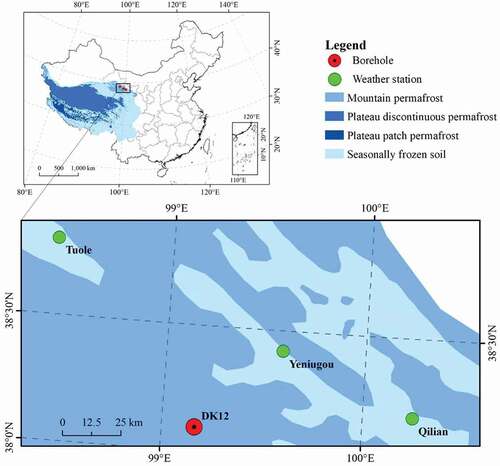
The borehole of DK-12 is located in Juhugeng of Muri Coalfield, Tianjun County, Qinghai Province, China, and is 600 m deep. The locations of the borehole and the nearby weather stations are shown in Figure 1, and some basic information concerning the borehole is listed in Table 1. The data set of DK-12 was chosen for this study not only because of its excellent T–z data but also because the borehole is situated in the mountain permafrost area (Wu, Zhang, and Liu 2010), where it is apparently free of ground water disturbance. This well can be used for several reasons: frozen ground of a permafrost area acts as the preferred medium of heat transfer and has recorded the past GST history, which can be reconstructed by solving an inverse heat conduction problem. The diameter of the borehole was 89 mm, and it was cased from the top to the bottom. After the cable was correctly placed, the space between the case and the cable was filled with dry sand. In addition, the depth of the borehole is great enough that surface temperature changes are attenuated such that the background thermal regime can be reliably determined.

Table 1. Basic information of the borehole

Borehole designation	Latitude (N)	Longitude (E)	Elevation (m)	Start time of drilling	End time of drilling	Permafrost thickness (m)	Temperature measurement time
DK-12	38°5′29.3″	99°10′16″	4,070	15 July 2014	10 October 2014	105.4	31 December 2017

Figure 1. Location of the DK-12 borehole (red point) and the nearby three weather stations (green points)

The temperature in the hole is measured by a cable of temperature sensors with an accuracy of ±0.05°C that were developed by the State Key Laboratory of Frozen Soil Engineering. Introduction of the temperature sensor and the recalibration test was described in detail by Shen, Liu, and Zhao (2012). The thermistor was a SKLFSE-TS (temperature sensor made at the State Key Laboratory of Frozen Soil). When it was manufactured in the laboratory, it was calibrated using a platinum resistance temperature sensor with an accuracy of ±0.01°C per national measurement standards. Each sensor in the cable was directly connected to the datalogger (Campbell CR3000) and they did not interact with each other.

Detailed information concerning the depths of all sensors in the cable is given in Table 2. The temperature sensor cable was installed on 6 November 2014. The cable, which was 600 m long and was held by a wireline, consisted of two strings, one for measuring the soil temperature from the ground surface to a depth of 300 m, another for measuring the soil temperature from a depth of 300 m to 600 m.

Table 2. Depths of the soil temperature sensors

Sensor no.	1	2	3	4	5	6	7	8	9	10	11	12	13	14	15
Depth (m)	0.5	1	1.5	2	2.5	3	3.5	4	4.5	5	5.5	6	6.5	7	7.5
Sensor no.	16	17	18	19	20	21	22	23	24	25	26	27	28	29	30
Depth (m)	8	8.5	9	9.5	10	11	12	13	14	15	16	17	18	19	20
Sensor no.	31	32	33	34	35	36	37	38	39	40	41	42	43	44	45
Depth (m)	25	30	35	40	45	50	60	70	80	90	100	110	120	130	140
Sensor no.	46	47	48	49	50	51	52	53	54	55	56	57	58	59	60
Depth (m)	150	160	170	180	190	200	210	220	230	240	250	260	270	280	290
Sensor no.	61	62	63	64	65	66	67	68	69	70	71	72	73
Depth (m)	300	310	320	330	360	390	420	450	480	510	540	570	600

The soil temperature at each depth listed in Table 2 were recorded by a datalogger twice a day at 12:00 a.m. and 12:00 p.m. from 7 November 2014 to 26 July 26 2015. From 27 July 2015 to 4 November 2016, the soil temperature at each depth was recorded every hour. From 5 November 2016 to present the soil temperature at each depth listed in Table 2 was recorded every 20 minutes. According to our monitoring data, the soil temperature was almost stabilized in June 2016 and was very stable after November 2016, which means that it took more than 1.5 years for the measuring environment to be stabilized after installation of the temperature cable. We used the temperature–depth log of the DK-12 borehole measured on 31 December 2017 to reconstruct the past GST history of the Muli area. Because this borehole is located close to the Yeniugou meteorological station, it is ideal for verifying the inversion results with air temperature observations from the Yeniugou station.

The upper 20 m of the temperature log was discarded in order to eliminate the annual temperature variation signal. Core samples were obtained to determine the underlying rock’s thermal diffusion coefficient. We selected the temperature profile of 420 m deep to contain the signal to allow for reconstruction of the climate during the past ~1,400 years.

Details on the borehole cores are listed in Table 3. These core samples were extracted during the drilling process. We did not directly measure the bulk thermal diffusivity from the core but use the average value of standard thermal diffusivity value of all layers of each lithology.

Table 3. Details of drilling core layers in borehole DK12

Layer no.	Top depth (m)	Bottom depth (m)	Lithology	Depth interval (m)
1	0	6.86	Clay deposits	6.86
2	6.86	58.37	Mudstone and sandstone interlayer	51.51
3	58.37	62.25	Breccia	3.88
4	62.25	165.55	Mudstone and sandstone interlayer	103.30
5	165.55	166.55	Breccia	1.00
6	166.55	172.80	Mudstone and sandstone interlayer	6.25
7	172.80	173.30	Coal	0.50
8	173.30	177.81	Sandstone	4.51
9	177.81	178.93	Conglomerate	1.12
10	178.93	211.20	Mudstone and sandstone interlayer	32.27
11	211.20	216.50	Coal	5.30
12	216.50	226.44	Mudstone and sandstone interlayer	9.94
13	226.44	408.14	Mudstone and oil shale interlayer	181.70
14	408.14	547.82	Mudstone	139.68
15	547.82	602.16	Mudstone and sandstone interlayer	54.34

In this study, we determined the long-term surface temperature and quasi-steady-state geothermal gradient by linear regression to the lowermost 120 m of the measured temperature profile. This linear regression represents the geothermal quasi steady-state from which the subsurface temperature anomalies are estimated. The anomaly $T\left(z\right)$ is obtained by subtracting this quasi-equilibrium thermal profile from the measured temperature profile. Figure 2 shows the measured temperature profile and its estimated subsurface temperature anomaly.

Figure 2. Temperature–depth profiles of the DK-12 borehole (blue lines) on 31 December 2017, shown as the blue line with points. Black lines represent the long-term background temperature profiles. The shaded area represents anomalous temperature resulting from surface ground temperature variation, and the values are represented by pink points that start below 20 m

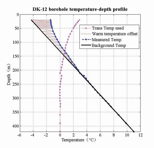
Figure 2 shows the general trend of past GSTvariation as the offset between measured and background T–z profiles. If there was a warm climate event, the GST increased and the transient temperature shifted toward the right, which caused a positive deviation in background temperature. In Figure 2 the red shaded area implies that a warm climate event appeared in the past. For details of past ground surface temperature trends we need to analyze the transient borehole temperature carefully. A conspicuous feature of the profiles in Figure 2 is the curvature in the upper 200 m. This curvature represents a systematic trend of warmer surface temperatures.

Model and method

Formulation of the problem

We used the same method as in Lachenbruch and Marshall (1986) to estimate the background temperature and separate the transient temperature. The general procedure has been to estimate and remove the background temperature by linear fitting. Because we do not know the exact ground surface temperature, we compared the measured ground temperature and the simulated ground temperature to indicate the accuracy of the reconstructed GST variation (Figure 3). In addition, the root mean square error (RMSE) between the measured and simulated ground temperature is an index to estimate the background temperature. We chose the best depth to separate background temperature from ground temperature by choosing the minimum value of RMSE. Here we use the average thermal diffusivity of each layer of the core.

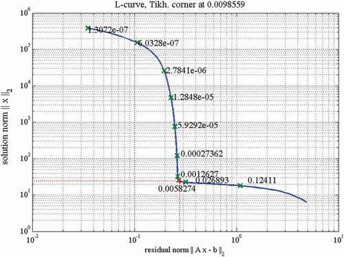
Figure 3. L-Curve rule for choosing the regularization parameter for Tikhonov regularization. The number in the L-curve are values of regularization parameters to imply the sensitive of results to regularization parameter

For a homogeneous, isotropic, source-free half-space, the temperature perturbation is the solution of the one-dimensional heat diffusion equation (Carslaw and Jaeger 1959)

(1) $\lambda \frac{{\mathrm{\partial }}^{2}T}{\mathrm{\partial }{z}^2}=\frac{\mathrm{\partial }T}{\mathrm{\partial }t},$(1)

where λ is the thermal diffusivity of the materials, z is depth (positive downwards), and t is time.

In the earth, the temperature perturbation is superimposed on the equilibrium temperature profile and can be determined as the difference between the measured temperature–depth profile and the long-term background temperature profile. By “long term” we mean the background thermal field that is affected by deep heat flow. We assume that the perturbation is mainly determined by the past GST variation history, although other factors such as surface water bodies, terrain, soil type, and vegetation can alter the shape of the T–z profiles. Because diffusion acts as a low-pass filter, short-term variations attenuate more quickly and are lost, and the past GST T₀(t) can be approximated by the average surface temperature during K time intervals of equal duration ∆; that is,

(2) ${\mathrm{T}}_0\left(\mathrm{t}\right)=T_k,\left(k-1\right)\mathrm{\Delta }\le t\le k\mathrm{\Delta }$(2)

Then the present temperature perturbation T(z) is given by (Vasseur et al. 1983)

(3) $\mathrm{T}\left({\mathrm{z}}_{\mathrm{j}}\right)={\sum }_{k=1}^K{T}_k{A}_{jk},$(3)

where T(z_j) is the calculated temperature perturbation at depth z_j and A_jk is a matrix element formed by evaluating the difference between complementary error functions at depth z_j and time t_k−1 = (k − 1)∆ and t_k = k∆:

(4) $A_{jk}=erfc\left\{\frac{z_j}{2\sqrt{\lambda t_{k-1}}}\right\}-erfc\left\{\frac{z_j}{2\sqrt{\lambda t_k}}\right\}.$(4)

Thus, we obtain an undetermined system of linear equations for T_k. We write Equation (4)(4) $A_{jk}=erfc\left\{\frac{z_j}{2\sqrt{\lambda t_{k-1}}}\right\}-erfc\left\{\frac{z_j}{2\sqrt{\lambda t_k}}\right\}.$(4) in matrix form:

(5) $\mathit{A}m=\mathit{d},$(5)

where

$\mathit{m}=\left(\begin{array}{c}{T}_1\\ T_2\\ ⋮\\ T_K\end{array}\right),\mathit{d}=\left(\begin{array}{c}T\left(z_0\right)\\ T\left(z_1\right)\\ ⋮\\ T\left(z_N\right)\end{array}\right)$

.

Here N is the total number of ground temperature measurement depths.

In order to suppress temperature oscillation in recent time we use time τ = ln(t) rather than normal time t. In τ time space, time points are denser near recent times and sparser toward the end. This adaptive time scheme allows us to have a high-resolution time interval for recent GST history. Because we set present time t₀ ≈ 0, we choose τ₀ = −18 to keep t₀ as t₀ = ln(τ₀) = ln(−18) ≈ 0. The time variable τ ranges from −18 to ln(tp) and has equal time step Δτ = 0.1.

Because this problem of inferring GST history from a borehole temperature profile is an inverse problem, the linear system is ill-posed and unstable and needs to be solved by regularization techniques. Mareschal and Beltrami (1992) used the generalized inverse method (Lanczos 1961) for this system of equations, which actually is the SVD regularization (Lanczos 1961; Jackson 1972; Menke 1989). In the next section, the linear system (3) is solved by Tikhonov regularization to reduce the impact of noise on the solution. For regularization parameter selection we chose the GCV method and the L-curve method.

Regularization technique

The large condition number of the matrix A makes it difficult to achieve good accuracy by standard numerical methods. For solving these ill-conditioned problems, several regularization methods have been developed (Hansen 1992a, 1992b, 1993, 2000; Hansen and O’Leary 1993). Here we adapt the Tikhonov regularization technique (Tikhonov and Arsenin 1979) to solve the matrix equation (5)(5) $\mathit{A}m=\mathit{d},$(5) . The Tikhonov regularization is to find the solution of the following optimization problem; that is, minimize the Tikhonov functional:

(6) ${min}_m\left\{||\mathit{A}m-d||{ }^2+{\alpha }^2||\mathit{m}||{ }^2\right\},$(6)

where ||∙|| is the usual Euclidean norm and α > 0 denotes the regularization parameter.

Now we need to choose a suitable value of the regularization parameter, a matter that is still of intensive research (Tikhonov and Arsenin 1979; Groetsch 1984; Engl, Hanke, and Neubauer 1996). In this simulation, we used the generalized cross-validation method and the L-curve method to determine the regularization parameter α.

The first investigations of the GCV method were done by Wahba (1977) and Craven and Wahba (1978) and more recently by Hansen (1992b, 1996). Rath and Mottaghy (2007) also applied the GCV method of selecting the regularization parameter to represent a trade-off between data fit and model smoothness. The GCV method involves choosing an optimal regularization parameter through minimizing the following GCV function:

(7) $\mathrm{G}\mathrm{C}\mathrm{V}\left(\alpha \right)=\frac{||\mathit{A}{\mathbf{m}}_{\alpha }-d|{|}^2}{{\left(\mathrm{t}\mathrm{r}\mathrm{a}\mathrm{c}\mathrm{e}\left(I_n-A\tilde{A}\right)\right)}^2},\alpha >0,$(7)

where $\tilde{\mathbf{A}}=({\mathbf{A}}^T\mathbf{A}+{\alpha }^2{I}_n{)}^{-1}{\mathbf{A}}^T$ is a matrix that generates the regularized solution when multiplied with d, i.e., ${\mathbf{m}}_{\alpha }=\tilde{\mathbf{A}}\mathbf{d}$

The L-curve regularization parameter criterion method was first developed by Lawson and Hanson (1995) and more recently by Hansen and O’Leary (1993). The L-curve method is sketched in the following. Define a curve L by

(8) $L=\{\left(log\left({∥{\mathbf{m}}_{\alpha }∥}^2\right)\right),\left(log\left({∥\mathbf{A}{\mathbf{m}}_{\alpha }-\mathbf{d}∥}^2\right)\right),\alpha >0\}.$(8)

The curve is known as an L-curve and a suitable regularization parameter α is the value near the “corner” of the L-curve (Hansen 1992a, 2000).

The matrix A in Equation (5)(5) $\mathit{A}m=\mathit{d},$(5) can be decomposed as

(7) $\mathit{A}=U\mathrm{\Lambda }{V}^T,$(7)

where U is the N × N orthonormal matrix formed by the vectors u^k spanning the input data space, V is the K × K orthonormal matrix formed by the vectors v^k that span the model parameter space, and Λ is an N × K diagonal matrix whose elements are the K singular values λ^k (Lanczos 1961). So all of the singular vectors v^k contain information of model parameters including the unknown GSTH values and measurement uncertainties. Then the solution of linear equation (5)(5) $\mathit{A}m=\mathit{d},$(5) can be written as m = A⁻¹d = VΛ⁻¹U^Td, where Λ⁻¹ is the diagonal matrix formed of the elements 1/λ^k or zeros when λ^k = 0.

The uncertainty of reconstructed GST history is calculated by taking the variance of the estimated parameters T_k. We calculate the variance based on singular vectors according to the regularization parameter α (Engl, Hanke, and Neubauer 1996):

(12) ${\sigma }_{Tikhonov,k}^2={\sum }_{j=1}^M\frac{{\left({\lambda }^k{v}_{\left(k\right)}^j\right)}^2}{{\left({\left({\lambda }^k\right)}^2+\alpha \right)}^2},$(12)

Here, M is the total number of singular values M = min(K, N), and $v_k^j$ is the kth value of singular vector $v^j$.

Results and discussion

The borehole temperature–depth profile was inverted to reconstruct the GST history for the past fourteen centuries. In this inversion problem, the ground acts as a low-pass filter in the heat diffusion process. There is a great loss of temporal resolution when the GST signal diffuses downward. The choice of a proper temporal parameterization is useful to reduce the error of inversion. This can be achieved by increasing the duration of the GST history model time intervals. For very long reconstructions, a logarithmic distribution has been used herein. The temporal length is smaller for the past 100 years than for the remote past, so the time resolution decreases as one goes back in time. The power of borehole temperature data to resolve past climatic events decreases with time due to the temporal smearing effect of ground temperatures. Therefore, it is important to quantify the degree of temporal smearing of the past climatic changes from measured borehole temperatures. We have introduced the Tikhonov method in detail in another work (Liu et al. submitted) and we found that reconstructed ground surface temperature (GST history) signal by the Tikhonov method provides the average real GST history of nearby 70 percent of the time in the past.

For the inversion, we used the Tikhonov method with a regularization parameter of 0.0099 chosen by the L-curve criterion method. Ground temperature can be forward modeled using Equation (3)(3) $\mathrm{T}\left({\mathrm{z}}_{\mathrm{j}}\right)={\sum }_{k=1}^K{T}_k{A}_{jk},$(3) to assess the fit of the Tikhonov method with respect to the measured borehole temperature. The RMSE between simulated and measured borehole temperature is computed to determine which regularization method to choose. The L-curve criterion showed a lower RMSE than the GCV method. In Figure 3 we illustrate the process of choosing the best regularization parameter by the L-curve criterion method, finally obtaining the optimal Tikhonov regularization parameter of 0.0099.

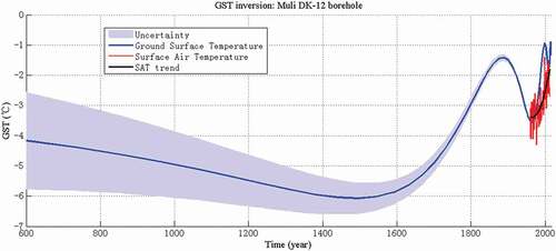
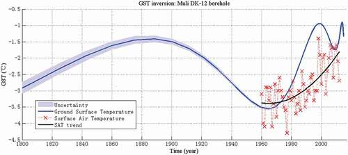
Figure 4. Estimated GSTH for the Muli area with the Tikhonov method from 600 to 2017 A.D. (blue line) and the surface air temperature measured from Yeniugou observation station (red line)

In this type of inversion, there is a great loss of temporal resolution because diffusion acts as a low-pass filter. Clow (1992) showed that each point comprising a GST history can be thought of as a running average where the window is at best about 50 percent of the time in the past. We found that the reconstructed GST signal by Tikhonov method provides the average real GST history of nearby 70 percent of the time in the past. From this point of view, the reconstructed GST is not the precise ground surface temperature of the time point but the general average of nearby 70 percent of the time. For example, a point 100 years ago represents an average surface temperature between 170 and 30 years ago. The inversion result is the GST trend of the past and the time resolution increases for earlier times. Therefore, our following conclusions should be considered from the perspective of average trends.

A total increase of ~3°C for the past fourteen centuries was observed at the borehole site. Figure 4 gives the GST history inferred by the Tikhonov method. The inversion results show that about 1,400 years ago the GST was about −4.1°C (±1.6°C). The reconstructed GST history we obtained is −4.1°C for the year 600. The inversion result not only shows the long-term GST history trend but also demonstrates the recent temperature fluctuation that was confirmed by the observed surface air temperature (SAT) from 1957 to 2012. A cooling trend of ~2°C was observed from 600 to 1500. The coldest periods around 1500 were identified, and this result was confirmed by Yang, Brauning, and Yafeng (2003). Then a clear warming transition was observed from the pre-industrial era (1500–1900) to the postindustrial era (1960–2000). The Little Ice Age cooling of ~2°C is shown between the years 1400 and 1600. Holmes, Cook, and Yang (2009) described the climate change over the past 2,000 years in western China, which showed the same climate fluctuation in the same time period (1400–1900). Then the abrupt drop in temperature around the 1960s was evident, which in agreement with the study by Zhang, Shugui, and Hongxi (2012). The average reconstruction suggests a rapid warming of ~2.5°C for the past 57 years. The temperature difference between the pre-industrial mean (1400–1500) and the mean between the years (1800–2017) is ~3.6°C.

The result by Holmes, Cook, and Yang (2009) shows temperature swings with a magnitude of approximately 1°C between 600 and 1400 when it dips to −1°C below the average at 1625 and then generally increases to 1.5°C at 1990 for a total amplitude of 2.5°C. The dip in the GST history at about 1500 agrees with Holmes, Cook, and Yang (2009) where the minimum is at 1625. However, the total warming found in the reconstructed GST history is about 5°C compared to the Holmes reconstructions of 2.5°C. These differences (two times more warming) may be due to two reasons. First, more warming may be caused by the regional differences and the research area may be more sensitive to climate changes. Second, the different techniques have different sensitivities to warming.

The surface temperature is warming in Yeniugou observations from 1960 to 2012. The GST history trend is consistent with instrumental surface air temperature measured from the Yeniugou observation station in the time period 1960 to 2012. The SAT trend from Yeniugou station also shows a mild SAT increase, in agreement with the GST history variation by our method. The reconstructed GST history shows a signal of temperature fluctuation in the period 2000 to 2017 (Figure 5). The SAT trend from Yeniugou station also shows an SAT oscillation during this period.

Figure 5. Detailed GST history for Muli area with the Tikhonov method from 1800 to 2017 A.D. (blue line) and the surface air temperature measured from Yeniugou observation station (red line)

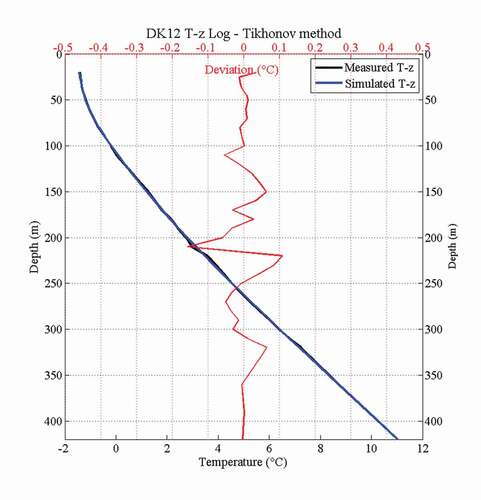
Figure 6 shows the T–z profile calculated from the estimated GST histories. Except for the shallow 20-m depth, the posteriori temperature values fall within 0.2°C of the measured values, with an RMSE of 0.04°C. The good fit between simulated and measured T–z log indicates the high degree of reliability of the Tikhonov method.

Figure 6. Measured (black line) and posteriori (blue line) T-z profiles for the DK-12 borehole data, corresponding to the GST histories by the Tikhonov method. The red line shows the deviation between measured and posteriori T-z profiles

The Muli borehole site shows that the warming trend intensified starting in the 1960s (Figure 5). Table 4 summarizes the total GST history variation we reconstructed by borehole paleothermometry from the DK-12 borehole as the average of the results.

Table 4. Climate change and geothermal gradient parameters from Muli DK-12 borehole

Borehole designation	T0 (°C)^a	Gradient (°C/km)	Inversion time (year)	Warmer (°C)	∆T (°C)^b	Tgr (°C)^c
DK-12	−4.16 (±1.57)	38.3 (±0.05)	~1400	2.86 (±0.08)	5.12 (±0.08)	−1.28 (±0.08)

Notes. ^aT₀ (°C) is the extrapolated equilibrium surface temperature (prior to climate change).

^b∆T (°C) gives the range of surface temperature variation.

^cT_gr (°C) is the present ground temperature determined by inversion.

The reconstructed GST history variations of Muli DK-12 exhibit the same trend as the SAT observations, but there is a temperature misfit. The borehole temperature reflects that the GST is, on average, warmer than the air temperature but that GST and SAT can vary with respect to each other because of changing ground conditions (Gosnold, Todhunter, and Schmidt 1997; Smerdon et al. 2004; Pollack, Smerdon, and Keken 2005). GST and SAT can change differently with time due to the different surface conditions, such as the timing and duration of seasonal snow cover, land use, vegetation development and changes, and soil moisture (Stieglitz et al. 2003; Bartlett, Chapman, and Harris 2004; Hu 2005; Smerdon et al. 2006, 2009).

On other hand, a major conclusion of Bartlett, Chapman, and Harris (2004) was that the timing and duration of seasonal snow cover act in concert (later snow cover usually means shorter duration) to minimally impact the coupling between air and ground temperature changes. Harris and Chapman (2005) showed that at the hemispheric scale, air and ground temperatures are well coupled. Further, given that winter temperatures are increasing more rapidly than summer temperatures and because multiproxy records of temperature change rely to a significant extent on tree ring data, which are sensitive to growing season (summer) temperatures, they miss the winter warming. In contrast, borehole records (and surface air temperature records) are sensitive to both winter and summer temperatures. Thus, it makes sense that borehole records of climate change show greater warming than multiproxy (or tree ring) records. Simply put, borehole temperature profiles are sensitive to both winter and summer temperatures, whereas tree ring records are mostly sensitive to growing season temperatures.

Summary

In this research, we used borehole paleothermometry to reconstruct GST variations in the Muli DK-12 borehole on the Qinghai–Tibet Plateau. We first utilized Tikhonov regularization in the borehole paleothermometry method. For the regularization parameter selection, we chose the L-curve method. The recent 67-year GST trend was consistent with the SAT variation trend obtained from the Yeniugou station, with value misfit resulting from local topography and ground surface energy budgets. Considering the above results, we conclude that the inversion results from the Muli DK-12 borehole display an increasing trend of ~3°C during the past ~1,400 years, and the major warming started in 1500. The inversion results of recent GST history fluctuations from 1960 to 2012 are confirmed by SAT observations of the Yeniugou Meteorological Station.

Acknowledgments

All of the authors appreciate the constructive advice from Professor Youhai Zhu and Dr. Shouji Pang during this work. We also appreciate the scientific research platform offered by Muli Field Scientific Observation and Research Station for Gas Hydrate, China Geological Survey.

Disclosure statement

No potential conflict of interest was reported by the authors.

Additional information

Funding

This research was supported by the open fund project of The Key Laboratory of Unconventional Oil & Gas Geology, CGS (Grant No. DD2019136-YQ19JJ01), the National Natural Science Foundation of China (Grant Nos. 41801029 and 41601073), the Natural Science Basic Research Plan in Shaanxi Province of China (Program No. 2018JQ4018), and the Fundamental Research Funds for the Central Universities (Grant No. 300102128101).

References

- Bartlett, M. G., D. S. Chapman, and R. N. Harris. 2004. Snow and the ground temperature record of climate change. Journal of Geophysical Research 109 (F4):F04008. doi:https://doi.org/10.1029/2004JF000224.
- Beck, A. E. 1977. Climatically perturbed temperature gradients and their effect on regional and continental heat-flow measurements. Tectonophysics 41 (1–3):17–39. doi:https://doi.org/10.1016/0040-1951(77)90178-0.
- Birch, F. 1948. The effects of Pleistocene climatic variations upon geothermal gradients. American Journal of Science 246 (12):729–60. doi:https://doi.org/10.2475/ajs.246.12.729.
- Bodri, L., and V. Cermak. 2011. Borehole climatology: A new method on how to reconstruct climate. Amsterdam: Elsevier.
- Carslaw, H. S., and J. C. Jaeger. 1959. Conduction of heat in solids. 2nd ed. Oxford, UK: Oxford University Press.
- Clow, G. D. 1992. The extent of temporal smearing in surface-temperature histories derived from borehole temperature measurements. Global and Planetary Change 6 (2):81–86. doi:https://doi.org/10.1016/0921-8181(92)90027-8.
- Craven, P., and G. Wahba. 1978. Smoothing noisy data with spline functions. Estimating the correct degree of smoothing by the method of generalized cross-validation. Numerische Mathematik 31 (4):377–403. doi:https://doi.org/10.1007/BF01404567.
- Dahl-Jensen, D., K. Mosegaard, N. Gundestrup, G. D. Clow, S. J. Johnsen, A. W. Hansen, and N. Balling. 1998. Past temperatures directly from the Greenland Ice Sheet. Science 282 (5387):268–71. doi:https://doi.org/10.1126/science.282.5387.268.
- Engl, H. W., M. Hanke, and A. Neubauer. 1996. Regularization of inverse problems. Netherlands: Springer Science & Business Media.
- Fernando, J. S., P. Carolyne, B. Hugo, and M. Jean-Claude. 2016. North American regional climate reconstruction from ground surface temperature histories. Climate of the Past 12 (12):2181–94. doi:https://doi.org/10.5194/cp-12-2181-2016.
- Gosnold, W., P. Todhunter, and W. Schmidt. 1997. The borehole temperature record of climate warming in the mid-continent of North America. Global and Planetary Change 15 (1):33–45. doi:https://doi.org/10.1016/S0921-8181(97)00002-7.
- Groetsch, C. W. 1984. The theory of Tikhonov regularization for Fredholm equations of the first kind. Boston, MA: Pitman (Advanced Publishing Program).
- Hansen, P. C. 1992a. Analysis of discrete ill-posed problems by means of the L-curve. SIAM Review 34:561–80. doi:https://doi.org/10.1137/1034115.
- Hansen, P. C. 1992b. Numerical tools of analysis and solution of Fredholm integral equations of the first kind. Inverse Problems 8 (6):849–72. doi:https://doi.org/10.1088/0266-5611/8/6/005.
- Hansen, P. C. 1993. Regularization tools: A Matlab package for analysis and solution of discrete ill-posed problems. Numerical Algorithms 14:1487–503.
- Hansen, P. C. 1996. Rank-deficient and discrete ill-posed problems. Lyngby, Denmark: Technical University of Denmark.
- Hansen, P. C. 2000. The L-curve and its use in the numerical treatment of inverse problem. In Computational inverse problems in electrocardiology. Advances in computational bioengineering series, ed. P. Johnston, vol. 4, 119–142. Southampton: WIT Press.
- Hansen, P. C., and D. P. O’Leary. 1993. The use of the L-curve in the regularization of discrete ill-posed problems. SIAM Journal on Scientific Computing 14 (6):1487–503. doi:https://doi.org/10.1137/0914086.
- Harris, R. N., and D. S. Chapman. 2001. Mid-latitude (30°N-60°N) climatic warming inferred by combining borehole temperatures with surface air temperatures. Geophysical Research Letters 28 (5):747–50. doi:https://doi.org/10.1029/2000GL012348.
- Harris, R. N., and D. S. Chapman. 2005. Borehole temperatures and tree rings: Seasonality and estimates of extratropical Northern Hemispheric warming. Journal of Geophysical Research Earth Surface 110 (F4):F04003.
- Holmes, J. A., E. R. Cook, and B. Yang. 2009. Climate change over the past 2000 years in Western China. Quaternary International 194 (1–2):0–107. doi:https://doi.org/10.1016/j.quaint.2007.10.013.
- Hon, Y. C., and T. Wei. 2004. A fundamental solution method for inverse heat conduction problem. Engineering Analysis with Boundary Elements 28 (5):489–95. doi:https://doi.org/10.1016/S0955-7997(03)00102-4.
- Hu, Q. 2005. How have soil temperatures been affected by the surface temperature and precipitation in the Eurasian continent? Geophysical Research Letters 32 (14):L14711. doi:https://doi.org/10.1029/2005GL023469.
- Huang, S., and H. N. Pollack. 1998. Global borehole temperature database for climate reconstruction. IGBP Pages/World Data Center—A for Paleoclimatology data contribution Series No. 1998-044. Boulder, CO: NOAA/NGDC Paleoclimatology Program.
- Huang, S., H. N. Pollack, and P. Y. Shen. 2000. Temperature trends over the past five centuries reconstructed from borehole temperatures. Nature 403 (6771):756–58. doi:https://doi.org/10.1038/35001556.
- Jackson, D. D. 1972. Interpretation of inaccurate, insufficient, and inconsistent data. Geophysical Journal International 28 (2):97–110. doi:https://doi.org/10.1111/j.1365-246X.1972.tb06115.x.
- Lachenbruch, A. H., and B. V. Marshall. 1986. Changing climate: Geothermal evidence from permafrost in Alaska. Science 234 (4777):689–96. doi:https://doi.org/10.1126/science.234.4777.689.
- Lanczos, C. 1961. Linear differential operators. New York: D. van Nostrand.
- Lawson, C. L., and R. J. Hanson. 1995. Solving least squares problems. SIAM. Philadelphia, PA: First published by Prentice-Hall.
- Liu, J., and T. Zhang. 2014. Fundamental solution method for reconstructing past climate change from borehole temperature gradients. Cold Regions Science and Technology 102:32–40. doi:https://doi.org/10.1016/j.coldregions.2014.02.005.
- Liu, J., T. Zhang, E. Jafarov, and G. D. Clow. Submitted. Application of Tikhonov regularization to reconstruct past climate record from borehole temperature: Synthetic cases.
- Majorowicz, J., S. E. Grasby, G. Ferguson, J. Safanda, and W. Skinner. 2006. Paleoclimatic reconstructions in western Canada from borehole temperature logs: Surface air temperature forcing and groundwater flow. Climate of the Past 2 (1):1–10. doi:https://doi.org/10.5194/cp-2-1-2006.
- Mann, M. E., S. Rutherford, R. S. Bradley, M. K. Hughes, and F. T. Keimig. 2003. Optimal surface temperature reconstructions using terrestrial borehole data. Journal of Geophysical Research 108 (D7):4203. doi:https://doi.org/10.1029/2002JD002532.
- Mareschal, J. C., and H. Beltrami. 1992. Evidence for recent warming from perturbed geothermal gradients: Examples from eastern Canada. Climate Dynamics 6 (3):135–43. doi:https://doi.org/10.1007/BF00193525.
- Menke, W., 1989. Geophysical data analysis. International Geophysical Series 45. San Diego: Academic Press.
- Pollack, H. N., and S. Huang. 2000. Climate reconstructions from subsurface temperatures. Annual Review of Earth and Planetary Sciences 28 (1):339–65. doi:https://doi.org/10.1146/annurev.earth.28.1.339.
- Pollack, H. N., S. Huang, and P.-Y. Shen. 1998. Climate change record in subsurface temperatures: A global perspective. Science 282 (5387):279–81. doi:https://doi.org/10.1126/science.282.5387.279.
- Pollack, H. N., J. E. Smerdon, and P. E. Keken. 2005. Variable seasonal coupling between air and ground temperatures: A simple representation in terms of subsurface thermal diffusivity. Geophysical Research Letters 32 (15):L15405. doi:https://doi.org/10.1029/2005GL023869.
- Rath, V., and D. Mottaghy. 2007. Smooth inversion for ground surface temperature histories: Estimating the optimum regularization parameter by generalized cross-validation. Geophysical Journal International 171 (3):1440–48. doi:https://doi.org/10.1111/j.1365-246X.2007.03587.x.
- Shen, Y., J. Liu, and S. Zhao. 2012. Long-term stability of thermometric thermistor sensor SKLFSE-TS used at low temperature. Journal of Glaciology and Geocryology 34 (4):891–97.
- Smerdon, J. E., H. Beltrami, C. Creelman, and M. B. Stevens. 2009. Characterizing land surface processes: A quantitative analysis using air‐ground thermal orbits. Journal of Geophysical Research: Atmospheres (1984–2012) 114 (D15). doi:https://doi.org/10.1029/2009JD011768.
- Smerdon, J. E., H. N. Pollack, V. Cermak, J. W. Enz, M. Kresl, J. Safanda, and J. F. Wehmiller. 2004. Air-ground temperature coupling and subsurface propagation of annual temperature signals. Journal of Geophysical Research: Atmospheres (1984-2012) 109 (D21). doi:https://doi.org/10.1029/2004JD005056.
- Smerdon, J. E., H. N. Pollack, V. Cermak, J. W. Enz, M. Kresl, J. Safanda, and J. F. Wehmiller. 2006. Daily, seasonal, and annual relationships between air and subsurface temperatures. Journal of Geophysical Research: Atmospheres (1984–2012) 111 (D7). doi:https://doi.org/10.1029/2004JD005578.
- Stieglitz, M., S. J. Dery, V. E. Romanovsky, and T. E. Osterkamp. 2003. The role of snow cover in the warming of arctic permafrost. Geophysical Research Letters 30 (13). doi:https://doi.org/10.1029/2003GL017337.
- Tikhonov, A. N., and V. Y. Arsenin. 1979. Methods for solving ill-posed problems. Scripta series in mathematics. Moscow: Nauka.
- Vasseur, G., P. H. Bernard, J. Van de Meulebrouck, Y. Kast, and J. Jolivet. 1983. Holocene palaeotemperatures deduced from geothermal measurements. Palaeogeography, Palaeoclimatology, Palaeoecology 43 (3–4):237–59. doi:https://doi.org/10.1016/0031-0182(83)90013-5.
- Wahba, G., 1977. A survey of some smoothing problems andthe method of generalized cross-validation for solvingthem. In Applications of Statistics: Proceedings of the Symposium Held at Wright State University, Dayton, Ohio, 14–18 June 1976, P. R. Krishnaiah (Ed), 507–23. Amsterdam: Elsevier.
- Wu, Q., T. Zhang, and Y. Liu. 2010. Permafrost temperatures and thickness on the Qinghai-Tibet Plateau. Global and Planetary Change 72 (1):32–38. doi:https://doi.org/10.1016/j.gloplacha.2010.03.001.
- Wu, Q., T. Zhang, and Y. Liu. 2012. Thermal state of the active layer and permafrost along the Qinghai-Xizang (Tibet) railway from 2006 to 2010. The Cryosphere 6 (3):607–12. doi:https://doi.org/10.5194/tc-6-607-2012.
- Yang, B., A. Brauning, and S. Yafeng. 2003. Late Holocene temperature fluctuations on the Tibetan Plateau (EI). Quaternary Science Reviews 22 (21):2335–44. doi:https://doi.org/10.1016/S0277-3791(03)00132-X.
- Yao, T., L. G. Thompson, V. Mosbrugger, F. Zhang, Y. Ma, T. Luo, B. Xu, X. Yang, D. R. Joswiak, W. Wang, et al. 2012. Third pole environment (TPE). Environmental Development 3:52–64. doi:https://doi.org/10.1016/j.envdev.2012.04.002.
- Zhang, Y., H. Shugui, and P. Hongxi. 2012. Preliminary study on spatiotemporal pattern of climate change over Tibet Plateau during past millennium. Marine Geology & Quaternary Geology 32 (3):135–146.