Vertical root distribution and biomass allocation along proglacial chronosequences in Central Switzerland

ABSTRACT

Investigating changes in belowground functional plant traits is an important step toward a better understanding of vegetation dynamics during primary succession. However, in alpine glacier forelands, we still lack an accurate assessment of plant rooting patterns. In this study, we established two proglacial chronosequences with contrasting bedrocks to investigate changes in rooting patterns and biomass allocation with terrain age. We extracted soil cores up to 1 m depth and measured root traits every 10 cm of each drilled core. Furthermore, we sampled aboveground biomass determining the contributions of functional groups to total aboveground biomass. We found that root traits associated with the root economics spectrum varied significantly along the chronosequences. Vertical root distribution coefficients revealed that early successional communities had more evenly distributed root systems compared to late successional communities. Biomass allocation showed diverging patterns. We found evidence for both the isometric allocation and optimal partitioning hypotheses. In addition, we observed a significant correlation between rooting parameters and plant community composition, suggesting that the dominance of distinct plant functional groups was one important factor explaining the observed rooting patterns. Our results shed light on the often neglected belowground compartments during plant succession and contribute to a better understanding of hillslope functioning.

KEYWORDS:

• Biomass allocation
• chronosequence
• glacier forelands
• root traits
• plant community composition

Introduction

Since the late Pleistocene, glaciers in alpine regions have been shrinking dramatically (e.g., Boxleitner et al. 2019). Former glacier positions can be identified by moraines representing distinct ages of substrate exposure (e.g., Egli, Fitze, and Mirabella 2001; Musso et al. 2019; Maier et al. 2020). This space-for-time substitution, called a chronosequence approach, enables scientists to test hypotheses related to terrain age. In glacier forelands, ecologists have frequently used this approach to study plant succession, which is defined as the turnover of species and communities over time in response to a disturbance (Matthews 1992; Walker and Del Moral 2003; Prach and Walker 2020).

Retreating glaciers expose young soils that have little biological legacy (Matthews 1992; Prach and Walker 2020). Such barren surfaces represent a very inhospitable habitat for early colonizers (Caccianiga et al. 2006). Although pioneer species must deal with high abiotic stress levels, such as low nutrients, extreme temperatures, and high ultraviolet radiation levels, vegetation cover and aboveground biomass are increasing quickly and a fully vegetated surface is normally observed after a few centuries (Matthews 1992; Walker and Del Moral 2003; Erschbamer and Caccianiga 2017). During succession in alpine glacier forelands, not only do cover and biomass change quickly but species composition does, too (Matthews and Whittaker 1987; Chapin et al. 1994; Raffl and Erschbamer 2004; Raffl et al. 2006; Robbins and Matthews 2009, 2010; Burga et al. 2010). Because of the site-specific differences in abiotic and biotic conditions, successional seres are known to be highly variable (Caccianiga and Andreis 2004; Schumann, Gewolf, and Tackenberg 2016). Nevertheless, patterns of vegetation dynamics show similarities in their main features. Young moraines are often covered by scree plant communities, followed by patches of initial grasslands and snowbed communities (Andreis, Caccianiga, and Cerabolini 2001). Subsequently, densely covered alpine grasslands are formed. Late successional communities in alpine glacier forelands often show elements of dwarf shrub communities or even subalpine forest stands, depending on elevation (Lüdi 1955, 1958; Burga et al. 2010). For example, because of more stressful conditions, on higher elevations, the speed and success of plant colonization, especially of shrub species, are reduced compared to lower elevations (Schumann, Gewolf, and Tackenberg 2016).

In addition to analyses of species turnover, trait-based approaches have increasingly gained attention for studying succession in recent years (Prach, Pyšek, and Šmilauer 1997; Fukami et al. 2005; Weppler and Stöcklin 2005; Caccianiga et al. 2006; Franzén et al. 2019). Functional traits reflect species’ strategies to meet the local requirements during succession, such as environmental conditions or spatiotemporal isolation. Therefore, investigating functional plant traits offers the potential to mechanistically understand the underlying ecological processes of succession (Schleicher, Peppler-Lisbach, and Kleyer 2011; Raevel, Violle, and Munoz 2012; Prach and Walker 2020). Until now, most research dealing with functional trait changes along successional gradients has focused on aboveground compartments of plants, whereas our understanding of belowground plant traits has lagged far behind (Holdaway et al. 2011; Erktan, McCormack, and Roumet 2018). However, belowground traits play a key role in understanding ecosystem functioning and for preserving ecosystem services (Bardgett, Mommer, and de Vries 2014; Garnier, Navas, and Grigulis 2016; Erktan, McCormack, and Roumet 2018). For instance, roots are involved in the regulation of plant–soil interactions (van der Putten et al. 2013), crucial for carbon as well as nutrient cycling (Hendricks, Nadelhoffer, and Aber 1993), and essential for maintaining slope stability (Freschet et al. 2017).

Two important belowground traits are specific root length (SRL, length of root per unit mass) and root tissue density (RTD, root mass per root volume). SRL and RTD are commonly used as equivalents to the functional leaf traits specific leaf area and leaf dry matter content (Ryser and Eek 2000; Ryser 2006; Freschet, Swart, and Cornelissen 2015). Because SRL and RTD are correlated with root life span, both are frequently used as key traits for the root economics spectrum (RES) hypothesis (Ryser 1996; Reich 2014; F. Li et al. 2019). Under the RES hypothesis, roots are assumed to follow a gradient in trait syndromes from fast foraging and short life span (acquisitive strategy) to slow foraging and long life span (conservative strategy; Freschet et al. 2010; Reich 2014; Kong et al. 2019). Such plant strategy types can be also identified using aboveground leaf traits (Hodgson et al. 1999; Wright et al. 2004). This approach has been tested on primary succession in glacier forelands, showing that pioneer communities are dominated by fast-growing species with high nitrogen leaf levels (Caccianiga et al. 2006). During succession, these species are progressively replaced by those with lower growth rates and denser leaves (Caccianiga et al. 2006; Gobbi et al. 2010). Theoretically, these findings should also apply to belowground traits when assuming that SRL and RTD behave like their aboveground equivalents.

Another belowground trait that is poorly investigated is vertical root distribution. This trait provides information about the morphology of rooting systems, which are highly plastic in response to abiotic and biotic changes and determine the efficiency of different rooting functions, such as water and nutrient uptake as well as anchoring in the soil (Bardgett, Mommer, and de Vries 2014). The spatial distribution of roots in the soil varies inter- and intraspecifically and reflects plant strategies of local adaptation to different physical and hydrological soil conditions (P. Hartmann and von Wilpert 2013). Furthermore, root distribution is linked to root architecture, which is known to influence hillslope functioning by creating networks of preferential flow (Ghestem, Sidle, and Stokes 2011; A. Hartmann et al. 2020). The most prominent model dealing with root distribution was proposed by Gale and Grigal (1987). It assumes an asymptotic relationship between root biomass and soil depth, as described by the extinction coefficient β. Gale and Grigal (1987) found that early successional tree species had the potential for a deep exploitation of the soil, which was hypothesized to be an adaptation to the homogenous distribution of nutrients and water in the substrate of early successional habitats. Jackson et al. (1996) and Schenk and Jackson (2002) conducted a global comparison of root distributions across different biomes, revealing that tundra, boreal forest, and temperate grasslands had the shallowest rooting profiles. Furthermore, they showed that plant functional groups differed significantly in their root systems, with grasses having 44 percent of their biomass allocated in the topsoil, followed by trees at 26 percent and shrubs at 22 percent. Consequently, communities consisting of different functional groups are suspected to exhibit distinct rooting patterns. Moreover, in diverse habitats, niche differentiation concerning resource requirements and uptake or species interactions may cause differences in rooting patterns compared to less diverse plant communities (de Kovel, Wilms, and Berendse 2000; Mommer et al. 2010; Poorter et al. 2012). In alpine habitats, however, studies on rooting systems are very scarce (Pohl et al. 2011). To our knowledge, there is no study on vertical root distribution development along chronosequences and, therefore, we lack a general understanding of how vertical root distribution changes during primary succession.

Measuring vertical root distribution enables researchers to calculate belowground biomass (BGB). If compared to the aboveground equivalent (AGB), this parameter provides information about biomass allocation, which is an important topic in plant ecology (McConnaughay and Coleman 1999; Poorter et al. 2012). In general, two contrasting hypotheses are debated (Shipley and Meziane 2002; McCarthy and Enquist 2007; Zeng, Wu, and Zhang 2015). The isometric allocation hypothesis assumes that AGB and BGB are related in an isometric manner; that is, the slope of the log–log relationship between AGB and BGB is not significantly different from one (Enquist and Niklas 2002; Niklas 2006; Yang et al. 2009). This is true for a diverse range of plant species and community types (Müller, Schmid, and Weiner 2000; Yang et al. 2009; Yang and Luo 2011). In contrast, according to the optimal partitioning hypothesis, plants respond to a gradient of environmental conditions (Nie et al. 2016; Dai et al. 2019, 2020) by allocating biomass among various organs to capture nutrients, water, and light (Bloom, Chapin, and Mooney 1985; Freschet et al. 2018). This hypothesis suggests that plants allocate more biomass to photosynthetic tissues under nutrient-rich conditions and invest more biomass into belowground organs in nutrient-poor conditions (McConnaughay and Coleman 1999). During primary succession, environmental conditions are expected to change considerably and a strong turnover of plant strategy types is observed (Caccianiga et al. 2006). In these habitats, biomass allocation should reflect the turnover of plant strategies and therefore optimal partitioning is expected during primary succession.

During primary succession, changes in root traits, root distribution, and biomass allocation are widely expected to occur, but both the patterns of these changes and their causes remain largely unexplored. The objective of this study was to shed light on the belowground features of plant succession. For this purpose, we examined the vertical root distribution and biomass allocation in two glacier forelands with distinct bedrocks. We also analyzed the influence of vegetation composition on vertical root distribution and root biomass. Chiefly, we tested the following hypotheses: (a) We expected that functional root traits vary along the chronosequences accordingly to the RES, indicating an acquisitive strategy at young moraines and a conservative strategy at old moraines. (b) We assumed that roots are more evenly distributed in early than in late successional habitats. (c) Due to the strong environmental heterogeneity along the chronosequences, biomass allocation patterns should follow the optimal partitioning hypothesis. (d) Finally, we hypothesized that vertical root distribution should be correlated with plant community composition.

Material & methods

Study sites

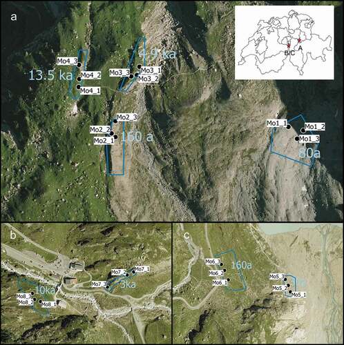
The present study made use of two long-term glacier foreland chronosequences with different bedrocks, each incorporating four moraines that span an age gradient from 30 a (a = years) to 13.5 ka (ka = thousands of years; Figure 1, Table 1; Musso et al. 2019). Both glacier forelands (Stein Glacier, Griess Glacier) are situated in Central Switzerland and are formed over siliceous and calcareous parent material. A summary of soil data along the two chronosequences is provided in Musso et al. (2019). An overview of some important vegetation characteristics is provided in Table 1. It is important to note that because of differences in species composition, the moraines represent different stages along the successional gradients.

1. Stein Glacier: This study site is located west of the Susten Pass in the Canton Bern (47°43′ N, 8°25′ E). The chronosequence of this site consisted of four moraines with estimated terrain ages of 30 a, 160 a, 3 ka, and 10 ka (Figure 1, Table 1). The four moraines of this site were dated in previous studies using radiocarbon dating, surface exposure dating as well as historical maps (Schimmelpfennig et al. 2014; Musso et al. 2019). The local bedrock at the Stein Glacier foreland is covered by glacial till on pre-Mesozoic silicate parent material, comprised of metamorphosed metagranitoids, gneisses, and amphibolites (Schimmelpfennig et al. 2014; Musso et al. 2019). All four moraines are situated above the timberline at elevations between 1,880 and 1,990 m.a.s.l. The soil types of this chronosequence were classified as Hyperskeletic Leptosols (30 a, 160 a) to Skeletic Cambisols (3 ka) and Entic Podzols (10 ka; Table 1; see also Musso et al. 2020).

2. Griess Glacier: This chronosequence is situated 25 km away from the Stein Glacier site. It is located near the Klausen Pass, in the glacier foreland of Griess Glacier, Canton Uri (46°50′ N, 8°49′ E). The moraines of the Griess Glacier foreland had estimated terrain ages of 80 a, 160 a, 4.9 ka, and 13.5 ka (Figure 1, Table 1). The determination of terrain ages of the moraines was done by radiocarbon dating of bulk soil and by using historical maps (Musso et al. 2019). In this glacier foreland, the deep-lying gneiss bedrock of the Griess Glacier is covered with limestone scree (Oechslin 1935; Musso et al. 2019). The elevation of the four moraines of this site is between 2,000 and 2,200 m.a.s.l. The soil types ranged from Hyperskeletic Leptosols (80 a, 160 a) to Calacaric Skeletic cambisols (4.9 ka, 13.5 ka; Table 1; see also Musso et al. 2020).

Table 1. Study site characteristics with terrain ages of the moraines, elevation, slope exposition, slope, bedrock, vegetation cover, species richness, and vegetation type of Stein Glacier (Susten Pass) and Griess Glacier (Klausen Pass) forelands

Moraine	Terrain age (years)	Elevation (m.a.s.l.)	Slope exposition (°)	Slope (%)	Bedrock	Soil type	Vegetation cover (%)	Species richness (n)	Vegetation type
Stein Glacier (Susten Pass, Central Switzerland)
30 a	30	1,990	ENE	40	Gneiss	Hyperskeletic Leptosol	49	23	Pioneer vegetation
160 a	160	1,990	ENE	31	Gneiss	Hyperskeletic Leptosol	98	43	Initial grassland and Salix shrubberies
3 ka	3,000	1,890	SW	25	Gneiss	Skeletic cambisol	94	33	Carex sempervirens grassland
10 ka	10,000	1,880	N	22	Gneiss	Entic Podzol	100	29	Rhododendron ferrugineum shrubberies and Nardus grassland
Griess Glacier (Klausen Pass, Central Switzerland)
80 a	80	2,200	WNW	27	Limestone	Hyperskeletic Leptosol	21	31	Pioneer vegetation
160 a	160	2,030	NE	31	Limestone	Hyperskeletic Leptosol	48	32	Scree vegetation
4.9 ka	4,900	2,010	N	37	Limestone	Calacaric Skeletic Cambisol	98	19	Carex ferruginea grassland
13.5 ka	13,500	2,000	NW	44	Limestone	Calacaric Skeletic Cambisol	100	11	Rhododendron hirsutum shrubberies and Carex ferruginea grassland

Figure 1. Location of (A) the Griess Glacier foreland (46°50′ N, 8°49′ E) and (B), (C) the lower and upper parts of the Stein Glacier foreland (47°43′ N, 8°25′ E). The terrain age of the moraines is given in years (a) and thousands of years (ka). Inset in (A) Switzerland with locations of both study sites. Satellite images: Google Maps, 2020, https://google.de/maps/place/Schweiz/@46.6192509,7.4679619.

Sampling strategy

On each moraine, we established three plots (each 4 m × 6 m) that were selected based on a structural vegetation complexity measure. Briefly, structural vegetation complexity was defined as an index based on vegetation cover and functional diversity data (Maier et al. 2020). Functional diversity was calculated based on the following eight traits characterizing species along the main axes of plant performance (Garnier, Navas, and Grigulis 2016): specific leaf area, nitrogen content, leaf dry matter content, Raunkiaeŕs life form, seed mass, clonal growth organ, root type, and stem growth form. For the plot selection, we conducted a vegetation mapping differentiating between vegetation units classified according to the characteristic recurrent combination of species. In each unit, we recorded all vascular plant species with proportion cover and calculated the vegetation complexity index. On every moraine, the three plots were placed within the surface units with the lowest, intermediate, and highest vegetation complexity.

On every plot, we conducted vegetation surveys, recording percentage plant cover of every single species by visual estimation. From these data, we calculated total plant cover and the cover of the different functional groups (grasses, forbs, shrubs). Species richness was computed as the total number of species per plot. Furthermore, we selected four 10 cm × 50 cm stripes and harvested AGB, distinguishing between grasses, forbs, and shrubs. The biomass samples were then dried (60°C, 72 hours) and weighed.

In addition, we extracted at least four soil cores per plot using a stainless steel soil column cylinder (diameter = 5 cm) that was drilled into the soil with a heavy, electrically powered percussion hammer (Makita HM 1800, Ratingen, Germany). The extracted cores were analyzed to a maximum core length of 1 m to maintain consistency. Each core was separated into 10-cm samples (0–10, 10–20, 20–30, 40–50, 60–70, 80–90, 90–100 cm). In total, we analyzed 394 samples at the Stein Glacier site and 432 samples at the Griess Glacier site. Sampling was done in July and August 2018 (Stein Glacier) and 2019 (Griess Glacier).

Processing and analyzing the roots

The roots were cleaned of soil and sorted into three diameter classes: <1 mm (i.e., fine roots), 1–2 mm (i.e., fibrous roots), and >2 mm (i.e., coarse roots). The samples were scanned in water with a flatbed scanner (Epson Perfection V700 Photo, Seiko Epson Corporation, Nagano, Japan, resolution 800 dpi). We used the software WinRHIZO Reg 2013e (Régent Instruments Inc. 2013) to measure the root length and root volume from the scans. Thereafter, each sample was dried (60°C, 72 hours) and weighed. To reduce workload, where more than ten scans would be necessary to capture all fine roots, material was subsampled.

For each sample, fine root mass density (FRMD), fine root length density (FRLD), SRL, and RTD were calculated (Table 2). FRMD and FRLD were obtained by dividing the root mass and root length, respectively, of the fine roots by the soil volume, which was determined by subtracting the volume of stones (mesh size of sieve >2 mm) from the volume of the corresponding soil cylinder. SRL was calculated as the length of fine roots per fine root mass of the sample and RTD as root mass per root volume of fine roots. Furthermore, we calculated the total root biomass by adding up the root dry weight of every soil depth increment and relating them to the area of 1 m² (Table 2).

Table 2. List of traits investigated in the present study

Root trait	Unit	Description
FRMD	g cm^−3	Dry weight of fine roots (diameter <1 mm) per unit soil volume
FRLD	cm cm^−3	Root length of fine roots (diameter <1 mm) per unit soil volume
SRL	cm g^−1	Root length per unit dry weight of fine roots
RTD	g cm^−3	Dry weight per root volume of fine roots
β		Measure for shallow and deep rooting, respectively: $Y=1-{\beta }^d$
BGB	kg m^−2	Belowground biomass
AGB	kg m^−2	Aboveground biomass
R:S ratio	%	Root-to-shoot ratio

Statistical analyses

As a first step, we calculated the per plot averages of all samples. To test hypothesis (a), we built linear mixed effect models. We used a three-way interaction of site (Griess Glacier, Stein Glacier), soil depth, and terrain age as fixed effects to investigate the changes of root traits (FRMD, FRLD, SRL, RTD) as a response of terrain age and soil depth. As such, soil depth was fitted as a factor variable. The affiliation of the plots to the moraines was included as a random term. To meet model assumptions, response variables were log-transformed. Linear mixed models were created using the R package lme4 (Bates et al. 2007). The model outputs are shown in Appendix S1.

To test hypothesis (b), we calculated the vertical root distribution coefficient according to the model of Gale and Grigal (1987):

$Y=1-{\beta }^d,$

where Y is the cumulative root fraction, d is the soil depth (cm), and β is the fitted extinction coefficient. The model suggests a nonlinear asymptotic relationship between root measures and soil depth. We used the fine root measures of FRMD and FRLD to calculate the cumulative root fraction (Y) for any 10-cm step from the surface to 1 m soil depth and derived the extinction coefficient (β). The cumulative root fraction represents the percentage of FRMD/FRLD from the soil surface to the depth considered relative to total FRMD/FRLD of the soil profile. The extinction coefficient β is a measure of vertical fine root distribution and may be interpreted as the allocation pattern of FRMD/FRLD. The values of β range from 0 to 1, where 1 indicates that the whole root biomass or root length, respectively, is located in deep soil and 0 indicates that the whole root biomass or root length, respectively, is concentrated at the surface.

To test the isometric allocation hypothesis (c), we performed simple linear models fitting log AGB as a function of log BGB. To investigate the change of AGB, BGB, and root-to-shoot (R:S) ratio along the chronosequences, we computed one-way analyses of variance and subsequent post hoc comparisons using the least significant difference (LSD) test. Significance levels were corrected according to the Bonferroni adjustment for multiple testing (Scheiner 1993).

The relationships between aboveground vegetation characteristics and vertical root distribution (hypothesis (d)) were analyzed using Pearson correlation coefficients. All analyses were performed with R version 3.5.1 (R Core Team 2018).

Results

Functional root traits along the chronosequences

The vertical distribution of the investigated functional root traits (FRMD, FRLD, SRL, RTD) showed large variations across all moraines and soil depths (Figure 2). At the Stein Glacier, FRMD ranged from 0 to 2.06 g cm⁻³, FRLD from 0.03 to 12.51 cm cm⁻³, SRL from 3.3 to 157.3 m g⁻¹, and RTD from 0.01 to 0.67 g cm⁻³. At the Griess Glacier, FRMD ranged from 0 to 3.35 g cm⁻³, FRLD from 0.02 to 24.68 cm cm⁻³, SRL from 6.5 to 200.0 cm g⁻¹, and RTD from 0.24 to 0.65 g cm⁻³ (Figure 2). Across all moraines, FRMD and FRLD decreased exponentially with soil depth (Figures 2a–2d). In the top 20 cm of the soil profiles, FRMD and FRLD were considerably higher on old moraines (2.21 g cm⁻³, 16.48 cm cm⁻³) than on young moraines (0.14 g cm⁻³, 1.58 cm cm⁻³). This finding was also reflected by positive effect sizes, indicating the rate of change with terrain age at certain soil depths (Figures 3a–3d). In the topsoil, SRL decreased, and deeper in the soil it increased with terrain age (Figures 2e and 2f, Figures 3e and 3f). An opposite pattern was observed for RTD, showing positive effect sizes in upper soil layers and negative effect sizes deeper in the soil (Figures 3g and 3h).

Figure 2. Vertical distributions of mean FRMD, FRLD, SRL, and RTD per soil depth increment across the moraines of (a), (c), (e), (g) Stein Glacier and (b), (d), (f), (h) Griess Glacier forelands. Error bars show the standard error of the mean. The terrain age of the moraines is given in years (a) and thousands of years (ka).

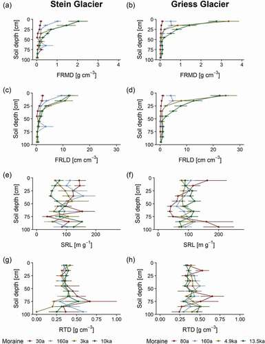
Figure 3. Effect sizes of FRMD, FRLD, SRL, and RTD of (a), (c), (e), (g) Stein Glacier and (b), (d), (f), (h) Griess Glacier forelands. Effect sizes indicate the rate of change of the root traits per 100 years of terrain age. The response variables are on a log scale.

β coefficients along the chronosequences

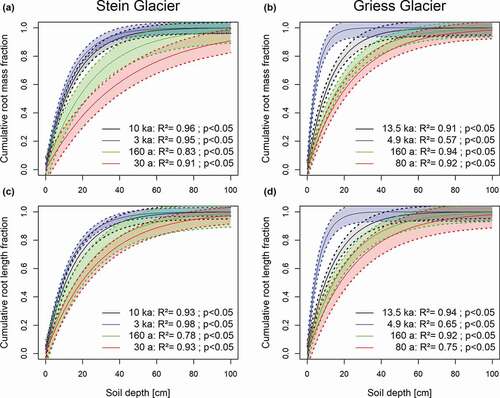
The vertical root distribution coefficient β ranged from 0.818 to 0.974 for FRMD and from 0.838 to 0.963 for FRLD (Table 3). At the Griess Glacier site, the coefficients changed significantly, whereas at the Stein Glacier site no significant changes were found. The coefficients showed a similar pattern along both chronosequences (Figure 4, Table 3). We found the highest β values at the 30 a, 80 a moraines and the lowest values at the 3 ka and 4.9 ka moraines (Figure 4, Table 3). On the oldest moraines of both sites, more than 90 percent of the root biomass was allocated in the uppermost 30 cm of soil, versus approximately 68 percent on the youngest moraines (Table 3).

Table 3. Mean vertical root distribution coefficient, β, and root fractions in the soil top 30 cm (RF_Top30cm) across the moraines of the study sites

Site	Moraine	βFRMD	RFTop30cm	βFRLD	RFTop30cm
Stein Glacier	30 a	0.974^a	70.15^a	0.961^a	54.61^a
Stein Glacier	160 a	0.942^a	80.63^a	0.947^a	83.22^a
Stein Glacier	3 ka	0.921^a	92.08^a	0.919^a	91.50^a
Stein Glacier	10 ka	0.936^a	87.38^a	0.933^a	86.09^a
Griess Glacier	80 a	0.961^a	67.46^b	0.963^a	69.71^b
Griess Glacier	160 a	0.956^a	72.53^b	0.958^a	73.68^ab
Griess Glacier	4.9 ka	0.818^b	99.50^a	0.838^b	99.76^a
Griess Glacier	13.5 ka	0.922^a	88.31^ab	0.931^a	91.34^ab

Notes. The model of Gale and Grigal (1987) was used to calculate β coefficients from FRMD and FRLD. A post hoc LSD test was conducted to compare root distribution measures among the moraines. The significance level was adjusted according to the Bonferroni method. Superscript letters indicate significant differences. The terrain age of the moraines is given in years (a) and thousands of years (ka).

Figure 4. Vertical distribution of (a), (b) root mass and (c), (d) root length across the moraines (see Table 1) of the (a), (c) Stein Glacier and (b), (d) Griess Glacier forelands. The vertical root distribution was fitted using the model proposed by Gale and Grigal (1987). The resulting β coefficients are shown in Table 4. The cumulative root fraction represents the percentage of roots from the soil surface to the depth considered relative to the total roots of the soil profile. Models are plotted showing the 95 percent confidence intervals.

Biomass allocation patterns along the chronosequences

AGB showed diverging patterns in the two glacier forelands. At the Stein Glacier site, AGB increased significantly along the chronosequence (Figure 5a), ranging from 0.16 to 1.29 kg m⁻² (Table 4). At the Griess Glacier foreland, it remained constant at around 0.40 kg m⁻² (Figure 5b, Table 4). Along both chronosequences, shrubs accounted for the largest proportions of AGB (Table 4). At the Stein Glacier foreland, the proportion of shrubs to total AGB increased with terrain age (except for the 3 ka), whereas grass and forb proportions decreased. At the Griess Glacier foreland, the proportion of grasses to total AGB increased with terrain age, forb proportion remained constant, and shrub proportion decreased (Table 4).

Table 4. Mean BGB, AGB, and R:S ratio across the moraines of the study sites

Site	Moraine	BGB (kg m^−2)(<1 mm/1–2 mm/>2 mm)	AGB (kg m^−2)(grasses/forbs/shrubs)	R:S ratio
Stein Glacier	30 a	0.16 (82/11/16)	0.16 (14/23/63)	0.96
Stein Glacier	160 a	0.99 (48/14/38)	0.84 (6/11/84)	1.18
Stein Glacier	3 ka	0.96 (82/10/8)	0.41 (28/51/20)	2.32
Stein Glacier	10 ka	2.29 (40/10/49)	1.95 (5/5/91)	1.17
Griess Glacier	80 a	0.09 (55/21/24)	0.44 (2/19/80)	0.22
Griess Glacier	160 a	0.37 (82/7/31)	0.34 (14/35/51)	1.07
Griess Glacier	4.9 ka	1.21 (75/9/15)	0.48 (37/17/46)	2.50
Griess Glacier	13.5 ka	2.03 (71/6/23)	0.38 (37/22/62)	5.29

Notes. Percentage contributions of root diameter classes (<1 mm, 1–2 mm, >2 mm) and functional groups (grasses, forbs, shrubs) are given in parentheses. The terrain age of the moraines is given in years (a) and thousands of years (ka).

Figure 5. AGB, BGB, and R:S ratio across different moraines and the relationships between AGB and BGB of (a), (c), (e), (g) Stein Glacier and (b), (d), (f), (h) Griess Glacier forelands. A post hoc LSD test was conducted to compare biomass measures among the moraines. The significance level was adjusted according to the Bonferroni method. Superscript letters indicate significant differences.

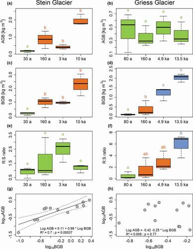
BGB increased along both chronosequences and showed significant changes across the moraines (Figures 5c–5d, Table 4). At the Stein Glacier site, BGB showed minimal values at the 30 a moraine (0.16 kg m⁻²), reaching maximal values at the 10 ka moraine (2.29 kg m⁻²; Table 4). Similarly, at the Griess Glacier site, BGB increased constantly from the youngest moraine (0.09 kg m⁻²) to the oldest moraine (2.03 kg m⁻²; Table 4). On young moraines (terrain age ≤160 a) of both sites, fine roots (<1 mm) accounted for the largest proportion of BGB. On old moraines (terrain age ≥3 ka), contributions to BGB depended on vegetation composition. Where grasses dominated, fine roots constituted the main percentage of BGB. In contrast, coarse root fraction (>2 mm) was highest where shrubs dominated (Table 4).

The R:S ratio showed a diverging pattern between the two study sites (Figures 5e–5f, Table 4). At the Stein Glacier site, the R:S ratio did not show significant changes between the moraines (range: 0.96–2.32; Figure 5e, Table 4), whereas at the Griess Glacier site, the R:S ratio increased significantly along the chronosequence (Figure 5f), ranging from 0.22 at the youngest moraine to 5.29 at the oldest moraine (Table 4).

At the Stein Glacier site, we found a significant relationship between log AGB and log BGB, with a slope of approximately one (R² = 0.7, p < .05, Figure 5g). At the Griess Glacier site, no such trend was observed (Figure 5h).

Correlations between rooting parameters and vegetation composition

The Pearson correlation matrix showed different correlations between β coefficients, BGB, and vegetation measures (Table 5). The AGB of grass species correlated negatively with β coefficients and positively with BGB (p < .05). We also found a significant positive correlation (p < .05) between BGB and AGB as well as between BGB and shrub cover (Table 5).

Table 5. Pearson correlation coefficients of vertical root distribution coefficients and vegetation composition

	βRD	βRLD	BGB
Species richness	−0.3	−0.35	0.23
AGB	−0.01	0.02	0.61
Grass AGB	−0.65	−0.59	0.54
Forb AGB	0.02	0.04	0.05
Shrub AGB	0.06	0.08	0.55
Vegetation cover	−0.33	−0.33	0.38
Grass cover	−0.29	−0.35	0.32
Forb cover	−0.25	−0.25	0.13
Shrub cover	−0.16	−0.13	0.57

Note. Bold numbers indicate significant correlations (p < .05).

Discussion

Functional root traits along the chronosequences

The large differences in root densities across the moraines are related to a set of parameters linked to terrain age. Because AGB and BGB are typically positively correlated, the observed increase in FRMD and FRLD should be a function of vegetation dynamics; for example, increasing plant cover and biomass along the chronosequences (Y. Li, Luo, and Lu 2008; Yang et al. 2009; Dai et al. 2019, 2020). Furthermore, various soil properties are known to influence root growth (Unger and Kaspar 1994; Ho et al. 2005). For example, an increase in bulk density leads to an increase in soil resistance, which can impede root penetration. Musso et al. (2019) and A. Hartmann et al. (2020) reported a strong gradient in bulk density along the chronosequences of Stein Glacier and Griess Glacier. According to Musso et al. (2019), bulk density showed values close to 2 g cm⁻³ on the youngest moraines, which is considered to be limiting for root growth (Unger and Kaspar 1994). With ongoing succession, bulk density decreased due to an accumulation of root biomass and organic matter (Musso et al. 2019, 2020). Such soils are richer in fine material and hence provide better conditions for roots to penetrate the substrate. Thus, we conclude that the observed root density patterns are an expression of both the increasing colonization of plants and the changing physical soil conditions.

Depending on soil depth, the results for RTD and SRL presented an ambiguous picture. In the topsoil of the youngest moraines (30 a, 80 a), the comparatively high values of SRL and the tendency for low RTD values reflect a fast water and nutrient uptake strategy of early colonizers (Caccianiga et al. 2006; Erschbamer and Caccianiga 2017). In contrast, species of late successional communities seem to invest more biomass into strengthening root tissues. This trait pattern supports the RES hypothesis postulating a gradient in trait syndromes from an acquisitive to a conservative strategy (Ryser 1996; Reich 2014; Kong et al. 2019; F. Li et al. 2019). Similarly, from a belowground perspective, our findings confirm the shift from ruderal to stress-tolerant plant strategies as being derived from aboveground traits along glacier foreland succession by Caccianiga et al. (2006). In deeper soil horizons, we found an opposite SRL/RTD pattern compared to the upper layers. Here, SRL increased and RTD decreased with terrain age, which could be attributed to physical soil conditions. Typically, bulk density increases with soil depth and on young moraines, with stony soils, it is expected to reach very high levels. In these habitats, roots of early colonizers might have to face a trade-off between resource acquisition and mechanical resistance (Freschet et al. 2020).

β coefficients along the chronosequences

The vertical root distribution coefficients β showed a pattern that was in accordance with our second hypothesis. We found evidence that early successional habitats in glacier forelands have more evenly distributed root profiles in contrast to late successional communities. Our findings suggest that vegetation of young moraines is adapted to sites with limiting resources because of the potential to exploit larger volumes of soil (Gale and Grigal 1987). We further assume that late successional vegetation develops shallow root systems to exploit the resources that are concentrated in the upper soil layers as a result of biocycling and soil development (Gale and Grigal 1987; Gao et al. 2014; Ma et al. 2020). The vertical root distribution coefficients β of this study covered a wide range of values compared to a great variety of biomes, from tundra ecosystems to sclerophyllous shrublands (Jackson et al. 1996). At the second oldest moraines (3 ka, 4.9 ka) of both glacier forelands, we found exceptionally low β coefficients, Here, a lot of tufted species occurred (e.g., Carex sempervirens, Festuca sp.), forming a dense net of roots in the upper soil layers. β values of the oldest moraines (10 ka, 13.5 ka) were similar to those of Yang et al. (2009) from grasslands of the Tibetan plateau. The vegetation of these moraines was characterized by alpine grassland species and dwarf shrubs (e.g., Rhododendron sp., Vaccinium sp.), which are known to have deep-growing roots (Kutschera and Lichtenegger 2002). These differences in vegetation composition might be a further explanation for the emerging root distribution patterns.

Biomass allocation patterns along the chronosequences

The development of biomass allocation patterns along the Griess Glacier chronosequence met our expectation that biomass allocation should follow the optimal partitioning hypothesis (Kang et al. 2013; Nie et al. 2016; Dai et al. 2019, 2020). In contrast, at the Stein Glacier site, we found support for the isometric allocation hypothesis, which has been confirmed by Yang et al. (2009), Yang and Luo (2011), and Peng and Yang (2016). The differences in the allocation patterns between the two study sites are because AGB scaled differently with terrain age: AGB remained constant at the Griess Glacier and increased at the Stein Glacier. At the latter site, the vegetation was composed of more woody species, producing higher amounts of AGB (de Kovel, Wilms, and Berendse 2000), which in turn resulted in a balanced R:S ratio. The comparatively high occurrence of species belonging to subalpine mesic dwarf shrub heathlands on siliceous bedrock has been attributed to a higher subsurface water availability compared to locations with calcareous bedrock (Michalet et al. 2002).

Percentage contributions of root diameter classes to total BGB were related to the community composition at certain moraines as reflected by the AGB fractions of grasses, forbs, and shrubs. The different proportions of coarse roots present in the soil are expected to have implications for hillslope functioning. Roots with a large diameter are known to create networks of preferential flow via root channels, thus affecting subsurface flow (Mitchell, Ellsworth, and Meek 1995; Ghestem, Sidle, and Stokes 2011). To illustrate that, at the Stein Glacier site, A. Hartmann et al. (2020) found different flow types at the different moraines, ranging from matrix flow at younger terrain ages to macropore flow via root channels at the oldest moraine.

Correlations between rooting parameters and vegetation composition

Concerning the relationship between vegetation characteristics and rooting parameters, we found evidence that the occurrence of distinct functional groups drove vertical root distributions, therefore supporting our fourth hypothesis. Grass species seemed especially influential to the rooting patterns due to their generally high root biomass allocation in the uppermost soil horizons (Jackson et al. 1996). Thus, we conclude that the functional group composition of the plant communities had a major influence on the development of root distribution and BGB. However, because we did not measure the distributions of available nutrients and water in the profiles, there is still some uncertainty about how abiotic factors shape the rooting patterns of such ecosystems.

Conclusions

This study is the first accurate assessment of rooting patterns including vertical root distribution along proglacial chronosequences. The presented data set is of interest for a broader understanding of functional root traits in alpine communities and provides comprehensive information on the hidden half of succession-related vegetation dynamics. We illustrated remarkable differences in rooting patterns of alpine plant communities growing along two alpine chronosequences. We found a strong variation in root traits along the successional gradients, which reflected a turnover of plant strategy types. Furthermore, we showed that plant community composition was correlated with the investigated root parameters. Our findings contribute to a deeper understanding of plant succession in glacier forelands and may also have implications for hillslope functioning in these areas. However, because we did not measure nutrient availability and water status, there remains some uncertainty as to whether plant composition or environmental conditions caused the site-specific patterns. Both nutrient and water resources in the soils are hypothesized to have a large impact on root characteristics and, therefore, we encourage the measurement of these parameters and their interrelations with root patterns in follow-up research.

Acknowledgments

We thank Thomas Michel and his team of the Alpin Center Sustenpass as well as Cècile Zemp from Hotel Klausenpasshöhe for accommodation and logistical support during the fieldwork. We thank Kyle Kovach for language editing.

Disclosure statement

No potential conflict of interest was reported by the authors.

Supplementary material

Supplemental material for this article can be accessed on the publisher’s website

Additional information

Funding

This research is part of the HILLSCAPE project (www.hillscape.ch), which is supported by the German Research Foundation (DFG project number 318089487; funding to MSL: SCHE 695/9-1) and the Swiss National Science Foundation (project grant number 200021E-167563/1). The article processing charge was funded by the Baden-Wuerttemberg Ministry of Science, Research and Art and the University of Freiburg in the funding programme Open Access Publishing.

References

- Andreis, C., M. Caccianiga, and B. Cerabolini. 2001. Vegetation and environmental factors during primary succession on glacier forelands: Some outlines from the Italian Alps. Plant Biosystems - an International Journal Dealing with All Aspects of Plant Biology 135 (3):295–310. doi:https://doi.org/10.1080/11263500112331350930.
- Bardgett, R. D., L. Mommer, and F. T. de Vries. 2014. Going underground: Root traits as drivers of ecosystem processes. Trends in Ecology & Evolution 29 (12):692–99. doi:https://doi.org/10.1016/j.tree.2014.10.006.
- Bates, D., D. Sarkar, M. D. Bates, and L. Matrix. 2007. The lme4 package. R Package Version 2 (1):74.
- Bloom, A. J., F. S. Chapin, and H. A. Mooney. 1985. Resource limitation in plants-an economic analogy. Annual Review of Ecology and Systematics 16 (1):363–92. doi:https://doi.org/10.1146/annurev.es.16.110185.002051.
- Boxleitner, M., S. Ivy-Ochs, M. Egli, D. Brandova, M. Christl, and M. Maisch. 2019. Lateglacial and early Holocene glacier stages - New dating evidence from the Meiental in central Switzerland. Geomorphology 340:15–31. doi:https://doi.org/10.1016/j.geomorph.2019.04.004.
- Burga, C. A., B. Krüsi, M. Egli, M. Wernli, S. Elsener, M. Ziefle, T. Fischer, and C. Mavris. 2010. Plant succession and soil development on the foreland of the Morteratsch glacier (Pontresina, Switzerland): Straight forward or chaotic? Flora 205:561–76. doi:https://doi.org/10.1016/j.flora.2009.10.001.
- Caccianiga, M., A. Luzzaro, S. Pierce, R. M. Ceriani, and B. Cerabolini. 2006. The functional basis of a primary succession resolved by CSR classification. Oikos 112:10–20. doi:https://doi.org/10.1111/j.0030-1299.2006.14107.x.
- Caccianiga, M., and C. Andreis. 2004. Pioneer herbaceous vegetation on glacier forelands in the Italian Alps. Phytocoenologia 34:55–89. doi:https://doi.org/10.1127/0340-269X/2004/0034-0055.
- Chapin, F. S., L. R. Walker, C. L. Fastie, and L. C. Sharman. 1994. Mechanisms of primary succession following deglaciation at Glacier Bay, Alaska. Ecological Monographs 64:149–75. doi:https://doi.org/10.2307/2937039.
- Dai, L., X. Guo, X. Ke, Y. Lan, F. Zhang, Y. Li, L. Lin, Q. Li, G. Cao, B. Fan, et al. 2020. Biomass allocation and productivity–richness relationship across four grassland types at the Qinghai Plateau. Ecology and Evolution 10 (1):506–16. doi:https://doi.org/10.1002/ece3.5920.
- Dai, L., X. Ke, X. Guo, Y. Du, F. Zhang, Y. Li, Q. Li, L. Lin, C. Peng, K. Shu, et al. 2019. Responses of biomass allocation across two vegetation types to climate fluctuations in the northern Qinghai-Tibet Plateau. Ecology and Evolution 9 (10):6105–15. doi:https://doi.org/10.1002/ece3.5194.
- de Kovel, C. F. G., Y. J. O. Wilms, and F. Berendse. 2000. Carbon and nitrogen in soil and vegetation at sites differing in successional age. Plant Ecology 149 (1):43–50. doi:https://doi.org/10.1023/A:1009898622773.
- Egli, M., P. Fitze, and A. Mirabella. 2001. Weathering and evolution of soils formed on granitic, glacial deposits: Results from chronosequences of Swiss alpine environments. Catena 45 (1):19–47. doi:https://doi.org/10.1016/S0341-8162(01)00138-2.
- Enquist, B. J., and K. J. Niklas. 2002. Global allocation rules for patterns of biomass partitioning in seed plants. Science 295 (5559):1517. doi:https://doi.org/10.1126/science.1066360.
- Erktan, A., M. L. McCormack, and C. Roumet. 2018. Frontiers in root ecology: Recent advances and future challenges. Plant and Soil 424 (1):1–9. doi:https://doi.org/10.1007/s11104-018-3618-5.
- Erschbamer, B., and M. S. Caccianiga. 2017. Glacier forelands: Lessons of plant population and community development. In Progress in Botany, ed. F. M. Cánovas, U. Lüttge, and R. Matyssek, vol. 78, 259–84. Cham: Springer International Publishing.
- Franzén, M., P. Dieker, J. Schrader, and A. Helm. 2019. Rapid plant colonization of the forelands of a vanishing glacier is strongly associated with species traits. Arctic, Antarctic, and Alpine Research 51 (1):366–78. doi:https://doi.org/10.1080/15230430.2019.1646574.
- Freschet, G. T., C. Roumet, L. Comas, M. Weemstra, A. Bengough, B. Rewald, R. Bardgett, G. B. Deyn, D. Johnson, J. Klimešová, M. Lukac, M. McCormack, I. Meier, L. Pagès, H. Poorter, I Prieto, N. Wurzburger, M. Zadworny, A. Bagniewska-Zadworna, and F. Schnabel. 2020. Root traits as drivers of plant and ecosystem functioning: Current understanding, pitfalls and future research needs. New Phytologist accepted. doi:https://doi.org/10.1111/nph.17072.
- Freschet, G. T., C. Violle, M. Y. Bourget, M. Scherer-Lorenzen, and F. Fort. 2018. Allocation, morphology, physiology, architecture: The multiple facets of plant above- and below-ground responses to resource stress. New Phytologist 219 (4):1338–52. doi:https://doi.org/10.1111/nph.15225.
- Freschet, G. T., E. M. Swart, and J. H. C. Cornelissen. 2015. Integrated plant phenotypic responses to contrasting above- and below-ground resources: Key roles of specific leaf area and root mass fraction. New Phytologist 206 (4):1247–60. doi:https://doi.org/10.1111/nph.13352.
- Freschet, G. T., J. H. C. Cornelissen, R. S. P. Van Logtestijn, and R. Aerts. 2010. Evidence of the ‘plant economics spectrum’ in a subarctic flora. The Journal of Ecology 98 (2):362–73. doi:https://doi.org/10.1111/j.1365-2745.2009.01615.x.
- Freschet, G. T., O. J. Valverde-Barrantes, C. M. Tucker, J. M. Craine, M. L. McCormack, C. Violle, F. Fort, C. B. Blackwood, K. R. Urban-Mead, C. M. Iversen, A. Bonis, L. H. Comas, J. H. C. Cornelissen, M. Dong, D. Guo, S. E. Hobbie, R. J. Holdaway, S. W. Kembel, N. Makita, V. G. Onipchenko, C. Picon-Cochard, P. B. Reich, E. G. de la Riva, S. W. Smith, N. A. Soudzilovskaia, M. G. Tjoelker, D. A. Wardle, and C. Roumet. 2017. Climate, soil and plant functional types as drivers of global fine-root trait variation. Journal of Ecology 105 (5):1182–96. doi:https://doi.org/10.1111/1365-2745.12769.
- Fukami, T., T. Martijn Bezemer, S. R. Mortimer, and W. H. van der Putten. 2005. Species divergence and trait convergence in experimental plant community assembly. Ecology Letters 8 (12):1283–90. doi:https://doi.org/10.1111/j.1461-0248.2005.00829.x.
- Gale, M., and D. F. Grigal. 1987. Vertical root distributions of northern tree species in relation to successional status. Canadian Journal of Forest Research 17 (8):829–34. doi:https://doi.org/10.1139/x87-131.
- Gao, Y., N. He, G. Yu, W. Chen, and Q. Wang. 2014. Long-term effects of different land use types on C, N, and P stoichiometry and storage in subtropical ecosystems: A case study in China. Ecological Engineering 67:171–81. doi:https://doi.org/10.1016/j.ecoleng.2014.03.013.
- Garnier, E., M.-L. Navas, and K. Grigulis. 2016. Plant functional diversity. Organism traits, community structure, and ecosystem properties. 1st ed. Oxford, UK: Oxford University Press.
- Ghestem, M., R. C. Sidle, and A. Stokes. 2011. The influence of plant root systems on subsurface flow: Implications for slope stability. BioScience 61 (11):869–79. doi:https://doi.org/10.1525/bio.2011.61.11.6.
- Gobbi, M., M. Caccianiga, B. Cerabolini, F. de Bernardi, A. Luzzaro, and S. Pierce. 2010. Plant adaptive responses during primary succession are associated with functional adaptations in ground beetles on deglaciated terrain. Community Ecology 11 (2):223–31. doi:https://doi.org/10.1556/ComEc.11.2010.2.11.
- Hartmann, A., E. Semenova, M. Weiler, and T. Blume. 2020. Field observations of soil hydrological flow path evolution over 10 millennia. Hydrology and Earth System Sciences 24 (6):3271–88. doi:https://doi.org/10.5194/hess-24-3271-2020.
- Hartmann, P., and K. von Wilpert. 2013. Fine-root distributions of Central European forest soils and their interaction with site and soil properties. Canadian Journal of Forest Research 44 (1):71–81. doi:https://doi.org/10.1139/cjfr-2013-0357.
- Hendricks, J. J., K. J. Nadelhoffer, and J. D. Aber. 1993. Assessing the role of fine roots in carbon and nutrient cycling. Trends in Ecology & Evolution 8 (5):174–78. doi:https://doi.org/10.1016/0169-5347(93)90143-D.
- Ho, M. D., J. C. Rosas, K. M. Brown, and J. P. Lynch. 2005. Root architectural tradeoffs for water and phosphorus acquisition. Functional Plant Biology 32 (8):737–48. doi:https://doi.org/10.1071/FP05043.
- Hodgson, J. G., P. J. Wilson, R. Hunt, J. P. Grime, and K. Thompson. 1999. Allocating C-S-R plant functional types: A soft approach to a hard problem. Oikos 85 (2):282–94. doi:https://doi.org/10.2307/3546494.
- Holdaway, R. J., S. J. Richardson, I. A. Dickie, D. A. Peltzer, and D. A. Coomes. 2011. Species‐and community‐level patterns in fine root traits along a 120 000‐year soil chronosequence in temperate rain forest. Journal of Ecology 99 (4):954–63. doi:https://doi.org/10.1111/j.1365-2745.2011.01821.x.
- Jackson, R. B., J. Canadell, J. R. Ehleringer, H. A. Mooney, O. E. Sala, and E. D. Schulze. 1996. A global analysis of root distributions for terrestrial biomes. Oecologia 108 (3):389–411. doi:https://doi.org/10.1007/BF00333714.
- Kang, M., C. Dai, W. Ji, Y. Jiang, Z. Yuan, and H. Y. H. Chen. 2013. Biomass and its allocation in relation to temperature, precipitation, and soil nutrients in inner Mongolia Grasslands, China. PLoS One 8 (7):e69561. doi:https://doi.org/10.1371/journal.pone.0069561.
- Kong, D., J. Wang, H. Wu, O. J. Valverde-Barrantes, R. Wang, H. Zeng, et al. 2019. Nonlinearity of root trait relationships and the root economics spectrum. Nature Communications 10 (1):2203. doi:https://doi.org/10.1038/s41467-019-10245-6.
- Kutschera, L., and E. Lichtenegger. 2002. Wurzelatlas mitteleuropäischer Waldbäume und Sträucher. Leopold Stocker Verlag Graz.
- Li, F., H. Hu, M. L. McCormlack, F. De Feng, X. Liu, and W. Bao. 2019. Community-level economics spectrum of fine-roots driven by nutrient limitations in subalpine forests. Journal of Ecology 107 (3):1238–49. doi:https://doi.org/10.1111/1365-2745.13125.
- Li, Y., T. Luo, and Q. Lu. 2008. Plant height as a simple predictor of the root to shoot ratio: Evidence from alpine grasslands on the Tibetan Plateau. Journal of Vegetation Science 19 (2):245–52. doi:https://doi.org/10.3170/2007-8-18365.
- Lüdi, W. 1955. Die Vegetationsentwicklung seit dem Rückzug der Gletscher in den mittleren Alpen und ihrem nördlichen Vorland. Ber. Geobot. Forsch. Inst. Rübel Zürich 36–68.
- Lüdi, W. 1958. Beobachtungen über die Besiedlung von Gletschervorfeldern in den Schweizeralpen. Flora 146:386–407. doi:https://doi.org/10.1016/S0367-1615(17)32526-0.
- Ma, R., F. Hu, J. Liu, C. Wang, Z. Wang, G. Liu, and S. Zhao. 2020. Shifts in soil nutrient concentrations and C: N: P stoichiometry during long-term natural vegetation restoration. PeerJ 8:e8382. doi:https://doi.org/10.7717/peerj.8382.
- Maier, F., I. van Meerveld, K. Greinwald, T. Gebauer, F. Lustenberger, A. Hartmann, and A. Musso. 2020. Effects of soil and vegetation development on surface hydrological properties of moraines in the Swiss Alps. Catena 187:1–17. doi:https://doi.org/10.1016/j.catena.2019.104353.
- Matthews, J. A. 1992. The ecology of recently-deglaciated terrain. A geoecological approach to glacier forelands. Cambridge, UK: Cambridge University Press (Cambridge studies in ecology).
- Matthews, J. A., and R. J. Whittaker. 1987. Vegetation succession on the Storbreen glacier foreland, Jotunheimen, Norway: A review. Arctic and Alpine Research 19:385–95. doi:https://doi.org/10.2307/1551403.
- McCarthy, M. C., and B. J. Enquist. 2007. Consistency between an allometric approach and optimal partitioning theory in global patterns of plant biomass allocation. Functional Ecology 21 (4):713–20.
- McConnaughay, K. D. M., and J. S. Coleman. 1999. Biomass allocation in plants: Ontogeny or optimality? A test along three resource gradients. Ecology 80 (8):2581–93.
- Michalet, R., C. Gandoy, D. Joud, J.-P. Pagès, and P. Choler. 2002. Plant community composition and biomass on calcareous and siliceous substrates in the northern French Alps: Comparative effects of soil chemistry and water status. Arctic, Antarctic, and Alpine Research 34 (1):102–13. doi:https://doi.org/10.1080/15230430.2002.12003474.
- Mitchell, A. R., T. R. Ellsworth, and B. D. Meek. 1995. Effect of root systems on preferential flow in swelling soil. Communications in Soil Science and Plant Analysis 26 (15–16):2655–66. doi:https://doi.org/10.1080/00103629509369475.
- Mommer, L., J. van Ruijven, H. de Caluwe, A. E. Smit-Tiekstra, C. A. M. Wagemaker, N. Joop Ouborg, G. M. Bögemann, G. M. Van Der Weerden, F. Berendse, and H. Kroon. 2010. Unveiling below-ground species abundance in a biodiversity experiment: A test of vertical niche differentiation among grassland species. Journal of Ecology 98 (5):1117–27. doi:https://doi.org/10.1111/j.1365-2745.2010.01702.x.
- Müller, I., B. Schmid, and J. Weiner. 2000. The effect of nutrient availability on biomass allocation patterns in 27 species of herbaceous plants. Perspectives in Plant Ecology, Evolution and Systematics 3 (2):115–27. doi:https://doi.org/10.1078/1433-8319-00007.
- Musso, A., K. Lamorski, C. Sławiński, C. Geitner, A. Hunt, K. Greinwald, and M. Egli. 2019. Evolution of soil pores and their characteristics in a siliceous and calcareous proglacial area. Catena 182:1–16. doi:https://doi.org/10.1016/j.catena.2019.104154.
- Musso, A., M. Ketterer, K. Greinwald, C. Geitner, and M. Egli. 2020. Rapid decrease of soil erosion rates with soil formation and vegetation development in periglacial areas. Earth Surface Processes and Landforms (45):2824–39. doi:https://doi.org/10.1002/esp.4932.
- Nie, X., Y. Yang, L. Yang, and G. Zhou. 2016. Above- and belowground biomass allocation in shrub biomes across the Northeast Tibetan Plateau. PLoS One 11 (4). doi: https://doi.org/10.1371/journal.pone.0154251.
- Niklas, K. J. 2006. A phyletic perspective on the allometry of plant biomass-partitioning patterns and functionally equivalent organ-categories. New Phytologist 171 (1):27–40. doi:https://doi.org/10.1111/j.1469-8137.2006.01760.x.
- Oechslin, M. 1935. Beitrag zur Kenntnis der pflanzlichen Besiedelung der durch Gletscher freigegebenen Grundmoränenböden. Ber Naturforsch Ges Uri 4:27–48.
- Peng, Y., and Y. Yang. 2016. Allometric biomass partitioning under nitrogen enrichment: Evidence from manipulative experiments around the world. Scientific Reports 6 (1):28918. doi:https://doi.org/10.1038/srep28918.
- Pohl, M., R. Stroude, A. Buttler, and C. Rixen. 2011. Functional traits and root morphology of alpine plants. Annals of Botany 108 (3):537–45. doi:https://doi.org/10.1093/aob/mcr169.
- Poorter, H., K. J. Niklas, P. B. Reich, J. Oleksyn, P. Poot, and L. Mommer. 2012. Biomass allocation to leaves, stems and roots: Meta-analyses of interspecific variation and environmental control. New Phytologist 193 (1):30–50. doi:https://doi.org/10.1111/j.1469-8137.2011.03952.x.
- Prach, K., and L. R. Walker. 2020. Comparative plant succession among terrestrial biomes of the World. Cambridge: Cambridge University Press (Ecology, Biodiversity and Conservation).
- Prach, K., P. Pyšek, and P. Šmilauer. 1997. Changes in species traits during succession: A search for pattern. Oikos 79 (1):201–05. doi:https://doi.org/10.2307/3546109.
- R Core Team. 2018. R: A language and environment for statistical computing. R foundation for statistical computing. Vienna, Austria. Accessed April 2, 2019. https://www.r-project.org/.
- Raevel, V., C. Violle, and F. Munoz. 2012. Mechanisms of ecological succession: Insights from plant functional strategies. Oikos 121:1761–70. doi:https://doi.org/10.1111/j.1600-0706.2012.20261.x.
- Raffl, C., and B. Erschbamer. 2004. Comparative vegetation analyses of two transects crossing a characteristic glacier valley in the Central Alps. Phytocoenologia 34:225–40. doi:https://doi.org/10.1127/0340-269X/2004/0034-0225.
- Raffl, C., M. Mallaun, R. Mayer, and B. Erschbamer. 2006. Vegetation succession pattern and diversity changes in a Glacier Valley, Central Alps, Austria. Arctic, Antarctic, and Alpine Research 38:421–28.
- Régent Instruments Inc. 2013. WinRHIZO 2013 Reg, user manual. Quebec City, QC: Régent Instruments Inc.
- Reich, P. B. 2014. The world-wide ‘fast–slow’ plant economics spectrum: A traits manifesto. Journal of Ecology 102 (2):275–301. doi:https://doi.org/10.1111/1365-2745.12211.
- Robbins, J. A., and J. A. Matthews. 2009. Pioneer vegetation on glacier forelands in southern Norway: Emerging communities? Journal of Vegetation Science 20:889–902. doi:https://doi.org/10.1111/j.1654-1103.2009.01090.x.
- Robbins, J. A., and J. A. Matthews. 2010. Regional variation in successional trajectories and rates of vegetation change on glacier forelands in south-central Norway. Arctic, Antarctic, and Alpine Research 42 (3):351–61. doi:https://doi.org/10.1657/1938-4246-42.3.351.
- Ryser, P. 1996. The importance of tissue density for growth and life span of leaves and roots: A comparison of five ecologically contrasting grasses. Functional Ecology 10 (6):717–23. doi:https://doi.org/10.2307/2390506.
- Ryser, P. 2006. The mysterious root length. Plant and Soil 286 (1):1–6. doi:https://doi.org/10.1007/s11104-006-9096-1.
- Ryser, P., and L. Eek. 2000. Consequences of phenotypic plasticity vs. interspecific differences in leaf and root traits for acquisition of aboveground and belowground resources. American Journal of Botany 87 (3):402–11. doi:https://doi.org/10.2307/2656636.
- Scheiner, S. M. 1993. MANOVA: Multiple response variables and multispecies interactions. Design and Analysis of Ecological Experiments 94:112.
- Schenk, H. J., and R. B. Jackson. 2002. The global biogeography of roots. Ecological Monographs 72 (3):311–28. doi:https://doi.org/10.1890/0012-9615(2002)072[0311:TGBOR]2.0.CO;2.
- Schimmelpfennig, I., J. M. Schaefer, N. Akçar, T. Koffman, S. Ivy-Ochs, R. Schwartz, R. Finkel, S. Zimmerman, and C. Schlüchter. 2014. A chronology of holocene and little ice age glacier culminations of the Steingletscher, Central Alps, Switzerland, based on high-sensitivity beryllium-10 moraine dating. Earth and Planetary Science Letters 393:220–30. doi:https://doi.org/10.1016/j.epsl.2014.02.046.
- Schleicher, A., C. Peppler-Lisbach, and M. Kleyer. 2011. Functional traits during succession: Is plant community assembly trait-driven? Preslia 83 (3):347–70.
- Schumann, K., S. Gewolf, and O. Tackenberg. 2016. Factors affecting primary succession of glacier foreland vegetation in the European Alps. Alpine Botany 126 (2):105–17. doi:https://doi.org/10.1007/s00035-016-0166-6.
- Shipley, B., and D. Meziane. 2002. The balanced-growth hypothesis and the allometry of leaf and root biomass allocation. Functional Ecology 16 (3):326–31. doi:https://doi.org/10.1046/j.1365-2435.2002.00626.x.
- Unger, P. W., and T. C. Kaspar. 1994. Soil compaction and root growth: A review. Agronomy Journal 86 (5):759–66. doi:https://doi.org/10.2134/agronj1994.00021962008600050004x.
- van der Putten, W. H., R. D. Bardgett, J. D. Bever, T. M. Bezemer, B. B. Casper, T. Fukami, P. Kardol, J. N. Klironomos, A. Kulmatiski, J. A. Schweitzer, et al. 2013. Plant–soil feedbacks: The past, the present and future challenges. Journal of Ecology 101 (2):265–76. doi:https://doi.org/10.1111/1365-2745.12054.
- Walker, L. R., and R. Del Moral. 2003. Primary succession and ecosystem rehabilitation. Cambridge: Cambridge University Press.
- Weppler, T., and J. Stöcklin. 2005. Variation of sexual and clonal reproduction in the alpine Geum reptans in contrasting altitudes and successional stages. Basic and Applied Ecology 6 (4):305–16. doi:https://doi.org/10.1016/j.baae.2005.03.002.
- Wright, I. J., P. B. Reich, M. Westoby, D. D. Ackerly, Z. Baruch, F. Bongers, J. Cavender-Bares, T. Chapin, J. H. C. Cornelissen, M. Diemer, et al. 2004. The worldwide leaf economics spectrum. Nature 428:821. doi:https://doi.org/10.1038/nature02403.
- Yang, Y., J. Fang, C. Ji, and W. Han. 2009. Above- and belowground biomass allocation in Tibetan grasslands. Journal of Vegetation Science 20 (1):177–84. doi:https://doi.org/10.1111/j.1654-1103.2009.05566.x.
- Yang, Y., and Y. Luo. 2011. Isometric biomass partitioning pattern in forest ecosystems: Evidence from temporal observations during stand development. The Journal of Ecology 99 (2):431–37. doi:https://doi.org/10.1111/j.1365-2745.2010.01774.x.
- Zeng, C., J. Wu, and X. Zhang. 2015. Effects of grazing on above- vs. below-ground biomass allocation of alpine grasslands on the Northern Tibetan Plateau. PLoS One 10 (8):e0135173. doi:https://doi.org/10.1371/journal.pone.0135173.