Arctic insect emergence timing and composition differs across thaw ponds of varying morphology

ABSTRACT

Freshwater ponds provide habitats for aquatic insects that emerge and subsidize consumers in terrestrial ecosystems. In the Arctic, insects provide an important seasonal source of energy to birds that breed and rear young on the tundra. The abundance and timing of insect emergence from arctic thaw ponds is poorly understood, but understanding these fluxes is important, given the role of insects in food webs and current rates of environmental change at high latitudes. We aimed to evaluate emerging insect communities from thaw ponds with different morphologies, identify environmental covariates influencing insect composition, and describe temporal changes in insect abundance. We collected environmental information and insects that emerged over two growing seasons and examined the phenology and taxonomic composition of insects arising from different pond classes: low centered polygon, small coalescent, large coalescent, and trough ponds. Our findings indicated no differences in the timing of total emergence across ponds of varying morphology. Community dissimilarity was primarily associated with center or margin habitat and variables that differed strongly among pond classes. These insects, which provide important provisions for various species of birds, are likely to experience changes in emergence phenology and composition due to ongoing, rapid warming in the region.

KEYWORDS:

• Arctic
• insect
• phenology
• subsidy
• thaw pond

Introduction

Arctic freshwater ecosystems provide diverse habitats for aquatic insects that can subsidize terrestrial ecosystems (Hobbie 1984; Paasivirta, Lahti, and Perätie 1988; Danks 2007; Burpee and Saros 2020). At lower latitudes, emerging insects contribute substantially to the energy transferred from aquatic to terrestrial species (Baxter, Fausch, and Saunders 2005), 10 percent to 98 percent of avian energy budget (Nakano and Murakami 2001), and 67 to 82 percent of avian diet (Iwata, Nakano, and Murakami 2003); specifically, many terrestrial consumers rely on aquatic insect emergence during the early growing season, when terrestrial production is low (Nakano and Murakami 2001; Sabo and Power 2002). Aquatic habitats in the Arctic produce insects that are often a high proportion of the avian diet (Holmes and Pitelka 1968; Custer and Pitelka 1978), and emergent insect availability may also influence avian habitat selection, reproductive success, or growth (Schekkerman et al. 2003; Cunningham, Kesler, and Lanctot 2016; Reneerkens et al. 2016). The provision of ecosystem subsidies, however, is highly variable across landscapes due to heterogeneity in physical and biological features, the type of boundary between habitats, and the nature of the subsidy itself (Marczak, Thompson, and Richardson 2007; Schriever, Cadotte, and Williams 2014; Jooste, Samways, and Deacon 2020). Changes in the timing of insect emergence from aquatic systems may decrease density and growth of consumers in adjacent terrestrial habitats (Sabo and Power 2002) or create phenological mismatches between emerging insects and their predators (Saalfeld et al. 2019). In the Arctic, subsidies from aquatic to terrestrial systems have not been well studied, and factors affecting insect emergence in these locations remain poorly understood (Burpee and Saros 2020).

Large seasonal fluctuations in temperature and light favor insect species with adaptations to freezing and brief arctic summer growing seasons (Danks, Kukal, and Ring 1994; Rautio et al. 2011). To take advantage of the short summer, midges and mosquitos at high latitudes emerge as early in the season as possible in order to reproduce before winter returns (Butler, Miller, and Mozley 1980; Danks, Kukal, and Ring 1994); early emergence is encouraged by solar heating in and above sediments that promote benthic primary production and insect development (Stanley and Daley 1976; Danks 2007; Rautio et al. 2011). In solar-heated habitats of shallow ponds and pond margins, insects take advantage of microclimates that may be 20°C to 30°C warmer than the ambient air temperature (Danks, Kukal, and Ring 1994), which helps advance phenology during brief growing seasons (Harper and Peckarsky 2006; Culler, Ayres, and Virginia 2015). Furthermore, pond morphology can affect thermal and energy budgets (Koch, Gurney, and Wipfli 2014; Koch et al. 2018), which may influence the composition and timing of emergence and the heterogeneity of resource pulses to predators (Bolduc et al. 2013; Sardiña et al. 2017).

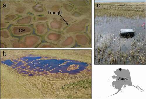
In addition to temperature, emergent aquatic insects may respond to multiple environmental drivers, including hydrology, hydroperiod (i.e., the length of the wetted season), habitat size, or nutrient availability (Greig et al. 2012; Schriever, Cadotte, and Williams 2014; Jonsson et al. 2015; Larsen, Muehlbauer, and Marti 2016). Various arctic thaw ponds provide heterogeneous habitats for aquatic, semiaquatic, and some terrestrial insects. Ponds (<10⁴ m²) vary in size and shape and are generally classified as (1) trough ponds that form in linear depressions above thawing ice wedges, (2) low centered polygon (LCP) ponds that form at the depressed centers of ice wedge polygons, and (3) coalescent ponds that form when permafrost thaws and trough and LCP ponds coalesce (Figure 1). LCP ponds are often ephemeral, wetting for a brief time during spring snowmelt flooding (Woo and Young 2006). Large, deep ponds are less likely to dry entirely and receive fewer nutrient-rich terrestrial inputs (Koch, Gurney, and Wipfli 2014). Trough ponds are unique, in that they sit atop ice wedges and are often significantly deeper than other pond types, resulting in inflows of subsurface water and thaw-derived nutrients (Koch, Gurney, and Wipfli 2014; Koch et al. 2018). Such diverse habitats likely support distinctive communities; empirical descriptions are lacking, however, on the composition of insects using arctic thaw ponds.

Figure 1. Thaw ponds of the Arctic Coastal Plain, Alaska: (a) low centered polygon (LCP) ponds form at the depressed centers of polygonal ground and trough ponds form above thawing ice wedges in cracks between polygons, (b) larger ponds form when permafrost thaws and multiple ponds of varying types coalesce, and (c) an emergence trap is positioned at the center of an LCP pond. All thaw ponds were sampled from a single study area indicated by the ♦ on the map of Alaska.

Arctic pond habitats are vulnerable to ongoing climate change, including increasing temperatures and altered precipitation regimes, which may affect insect development and potentially contribute to mismatched timing of subsidies to the terrestrial environment (Danks, Kukal, and Ring 1994; Høye and Forchhammer 2008; Rautio et al. 2011; Greig et al. 2012; Anderson, Albertson, and Walters 2019). Warming in wet regions of the Arctic Coastal Plain of Alaska has increased ground thaw depth, evaporation rates, and vegetated cover, which has led to a decrease in size and number of LCP ponds (Andresen and Lougheed 2015). Conversely, because of ice wedge degradation, the number of trough ponds has increased (Jorgenson et al. 2015; Liljedahl et al. 2016). The fate of coalescent ponds is difficult to predict given their range in size and morphologies but will similarly be impacted by interactions between permafrost thaw, altered hydrology, and ecosystem dynamics (Jorgenson et al. 2015; Koch et al. 2018). This shift in the relative abundance of trough and LCP ponds could influence the abundance or composition of aquatic insect species. Loss of water from ponds via changes in hydrological processes and changes in the terrestrial plant community (Woo and Young 2006; Jorgenson et al. 2015) could shift insect communities toward terrestrial species (Sim et al. 2013). Warming may also increase the number or biomass of emergent insect taxa from ponds (e.g., Bolduc et al. 2013; Sardiña et al. 2017) and advancement of spring thaw may promote earlier emergence (e.g., Saalfeld et al. 2019), yet factors that influence emergent insect communities in the Arctic remain poorly understood (Høye and Forchhammer 2008).

In this study, we aimed to evaluate variation in insect communities that emerged from thaw ponds of different morphologies: trough, LCP, small coalescent, and large coalescent ponds. Our specific objectives included (1) evaluating differences in the phenology, abundance, and composition of emerging insect communities within and between pond classes and (2) identifying key environmental covariates and their associations with pond morphology that influenced variation in insect community composition. We anticipated greater insect abundance emerging from warmer ponds with higher potential productivity (Danks and Oliver 1972; Hobbie 1984) and anticipated differences in composition across pond center and margin habitats (Butler, Miller, and Mozley 1980; Paasivirta, Lahti, and Perätie 1988; Loskutova 2020) and that this would relate to differences associated with pond volume and desiccation.

Methods

Study area

This study was conducted in 2012 and 2013 in thaw ponds on the central Arctic Coastal Plain (70°41′ N, 155°18′ W), a relatively flat, low-elevation area of sedge, moss, dwarf shrub wetland (CAVM Team 2003) between the Brooks Range foothills and the Beaufort Sea. The region’s climate and permafrost dynamics are responsible for the formation of substantial microtopography, including polygonal ground and ice wedges (Jorgenson and Shur 2007) and subsequently thaw lakes and ponds. The tundra is saturated during the spring snowmelt period and ponds provide numerous wetland habitats for aquatic insects. Mean daily air temperatures at the U.S. Geological Survey’s Ikpikpuk meteorological station (Urban and Clow 2016), 44 km to the southeast, first rose above freezing on 1 June 2012 and 20 May 2013 (Figure S1a). The first measurable rainfall at the meteorological station occurred on 25 June 2012 and 8 June 2013 (Figure S1b). Half as much rain fell during summer 2012 (45.6 mm) compared to the same time period in 2013 (90.9 mm), causing many of the shallow thaw ponds to dry by mid-July in 2012 (Koch, Gurney, and Wipfli 2014; Urban and Clow 2016). The final date of snowmelt, which was visually assessed in the field, occurred on 30 June 2012 and 25 June 2013 (Gurney and Uher-Koch 2012; Uher-Koch, Gurney, and Ruthrauff 2013).

Sample collection and processing

Three ponds each of LCPs, small coalescent (<50 m diameter), large coalescent (50–150 m diameter), and troughs were randomly selected from the study area, a location bounded using geographic information systems (ArcMap, ESRI, Redlands CA). No fish were observed in any of the ponds during regular visits over the course of the summer. For the purpose of trapping adult insects as they emerged from study ponds (n = 12) we deployed one floating emergence trap in the approximate pond center and tethered the trap in place using rebar anchors (Figure 1c; Cushman 1983). At a random subsample of ponds (n = 8), a second emergence trap was placed in the pond margin between wetted and dry habitats. Each trap (33 cm diameter) was fitted with a removable Petri dish (14 cm diameter) coated with Tree Tanglefoot (Tanglefoot Company, Grand Rapids, MI), a sticky substance that captures emerging insect adults. We collected samples every fourteen days in 2012 and every ten days in 2013, replacing each Petri dish and storing samples as soon as possible in a cool dark location for later processing. Traps were initially deployed on 29 June 2012 and 10 June 2013. Final collections were made on 11 August in 2012 and 1 August in 2013 (total number of samples in Table 1).

Table 1. Total number of floating insect emergence traps deployed in pond centers and margins of the different pond classes during summer 2012 and 2013

Pond class	Year	n Center	n Margin
Large coalescent	2012	9	3
	2013	13	0
Small coalescent	2012	9	6
	2013	14	10
Polygon	2012	9	3
	2013	15	5
Trough	2012	9	0
	2013	15	4

Each Petri dish was placed on a marked grid (2 × 2 cm) and the insects in each cell were identified (to family level, where possible) and counted under a dissecting microscope. When a complete census of trapped adults was not feasible due to high abundance (>500 individuals), a random subset of cells (n = 13, excluding partial cells along the rounded edge) was counted; total sample counts were obtained by summing all estimated values for a given taxon. All available data on insect emergence used in this publication can be found in Laske and Gurney (2021).

Variables were measured to determine correlations between the physical habitat and productivity of the thaw ponds and insect emergence. Pond volume was determined by multiplying the average pond depth, determined from multiple depth measurements made with a graduated D-frame kick net, and by pond area, determined using a tape measure for smaller ponds or based on area determined with a recreation-grade Global Positioning System (Garmin Oregon 550 t, Garmin International, Inc., Olathe, KS) for larger ponds. Water temperature was collected using a portable temperature logger (Hobo Tidbit V2, Onset Computer Corporation, Bourne, MA) suspended at mid-depth in the water column of each pond, following spring thaw of surface water but prior to beginning of insect collection (9 June to 15 June). Exposure to sunlight may have caused sensors to read artificially elevated water temperatures (Johnson and Wilby 2013), but consistency of the deployment method enabled us to make comparisons across pond classes. Any known exposures to air temperatures, such as exposed logger at the time of a pond visit, were removed from the final data set. The number of growing degree days (GDD) was determined by summing successive measurements of daily mean temperature from a common starting point (15 June, day of year [DoY] 166).

Water quality was measured in the field using a YSI-6920 (YSI, Inc., Yellow Springs, OH) water quality sensor that measured water temperature, pH, dissolved oxygen (DO), and specific conductance (EC). The probe was calibrated each day of sampling and allowed to equilibrate in each pond before taking a reading. Water quality samples were also collected and analyzed for nitrogen species (TDN, NH₄⁺; nitrate and nitrite were generally below detection levels), phosphorus (TDP), benthic and pelagic ash-free dry mass (bAFDM and pAFDM), and benthic and pelagic chlorophyll-a (bChla, pChla; see Koch, Gurney, and Wipfli [2014] for additional methods). AFDM and Chla in the benthic zone were collected using a small (14 cm diameter) plastic plate that was suspended just above the sediment–water interface. A raw water sample was collected at each pond and stored in a cool, dark location on the order of hours until returning to camp at the end of the day. A known volume of sample was filtered through a glass fiber filter. Nutrient samples (including nitrogen and phosphorus species) were stored in a 125 mL amber high-desnity polyethylene bottle. The glass fiber filter was stored in an aluminum foil envelope. All samples were stored in a cool dark location on-site for days to weeks until transportation was available to take them out of the field. The nutrient species samples were shipped to the U.S. Geological Survey National Water Quality Laboratory for analyses. The glass fiber filters were shipped to the Kiowa Laboratory at the Institute of Arctic and Alpine Research at the University of Colorado for analyses. Measurements of pond size, water volume, water chemistry, nutrient levels, and autotroph abundance (as indexed by AFDM and chlorophyll-a) were repeated during each of three to six resampling events (visits), between 19 June and 4 August 2013. All environmental data used in the analyses of this publication are available through U.S. Geological Survey data release (Koch et al. 2019).

Analytical methods

Emergence phenology

Using a series of hierarchical generalized additive models (R package mgcv, version 1.8; Wood 2017), we determined seasonal patterns of total insect emergence across the four classes of arctic ponds. Insect counts from each trap were standardized to account for surface area and the number of days the trap was deployed. We compared three models to determine whether and how emergence patterns varied across the pond classes: (1) a global smoother that is common for all observations, number ~ s(DoY) + s(Class) + s(Class, Year), (2) a global smoother plus group-level smoothers with a shared penalty, number ~ s(DoY) + s(DoY, Class) + s(Class, Year), and (3) a global smoother plus group-level smoothers with individual penalties, number ~ s(DoY) + s(Class) + s(DoY, by = Class) + s(Class, Year). The penalties in (2) and (3) influence the “wiggliness” of the curves: when the penalty is shared, group-level smoothers have similar wiggliness; when the penalty is not shared, group-level smoothers may have different wiggliness (Pedersen et al. 2019).

Over the short summer growing season, we expect the relationship between time and emergence to respond either linearly (zero, positive, or negative slope) or as a quadratic function (peaking at some point during the growing season; e.g., Anderson, Albertson, and Walters 2019); therefore, we used a cubic regression spline. The splines had basis complexity (k) of six for the day of year (i.e., s(DoY)) and three for day of year in class (i.e., s(DoY, Class)). Pond class (i.e., s(Class)) and the year in pond class (i.e., s(Class, Year)) were considered random effects. Emergence was modeled using a gamma distribution with a log-link, which does not permit zero-value data; therefore, zeroes (n = 2) were replaced with a low-value positive number (1 × 10⁻⁵; see Pedersen et al. 2019). Diagnostics plots and values for the fitted generalized additive models revealed reasonable fit and no evidence of oversmoothing. The fit of the three models was compared using the Akaike information criterion for small sample sizes (AICc; Burnham and Anderson 1998).

Composition

Emergence trap captures were evaluated at the taxonomic family level for all organisms. Any organisms that could not be identified to family (3 percent of individuals) and any captured larva (nonemergent) were removed from the analysis. We determined the number and identities of families observed in each pond class. In each sample, counts of insect families were standardized for area and the number of days the trap was deployed. We then looked at summary statistics across the pond classes and determined mean density by taxonomic family and origin (i.e., aquatic, semiaquatic, and terrestrial). Origin was determined from the literature (Borror, Triplehorn, and Johnson 1989; Merrit, Cummins, and Berg 2008). The ordination of community data was performed using nonmetric multidimensional scaling (NMDS) on Bray-Curtis dissimilarities using k = 3 dimensions (R package vegan version 2.5–5; Oksanen et al. 2019) at three sequential ten-day time periods beginning in early July 2013. The ten-day periods coincided with trap deployment and allowed us to investigate community correlations with the environment (see Environmental correlates section). To attain model convergence and reduce stress, density data were square root transformed and submitted to Wisconsin double standardization in period 1 and period 3 and square root transformed and standardized to the species maximum in period 2. Sixteen unique communities (i.e., assemblage for pond × habitat) were included in the analysis. One exception occurred in period 1, where only fourteen unique communities were included due to zero captures (small coalescent) or missing data (large coalescent). Insect families that occurred only once within the sample period were removed from the analysis, leaving seven, nine, and ten insect families, respectively, in periods 1, 2, and 3.

Environmental correlates

The environment during the 10-day period of insect collection was measured as the mean of the initial value (i.e., the day the trap was deployed) and the final value (i.e., the day the trap was collected). Only GDD was considered cumulatively, and the value on the final day was used. Water chemistry data below the detection limit were set to half of the detection limit for analyses. Low water levels did not permit water sampling in three ponds on at least one occasion; we interpolated values for (1) a small coalescent pond in period 3 by using values collected only at the time of trap placement and for (2) one LCP in period 2 and period 3 by using the mean value from surrounding measurements collected at the start of period 2 and ten days after the end of period 3 (except bAFDM, pChla, and bChla, which were missing). One LCP was completely excluded from the environmental analysis due to missing data prior to and after insect collection.

Environmental vectors and factors were fit to the community ordinations (R package vegan version 2.5–5; Oksanen et al. 2019), and permutation tests were used to determine the fit and significance of the variables for all k dimensions. We excluded variables that contributed little to explaining the ordination of pond insect communities and retained only those with false discovery rate corrected p value <0.10. We considered thirteen potential variables: bAFDM, pAFDM, bChla, pChla, DO, EC, GDD, NH₄⁺, TDN, TDP, pH, volume, and habitat (pond center or margin). Among the environmental variables, highly correlated variable pairs (|r| > 0.7), which responded in concert with one another, were removed from analyses by selecting only one variable from the pair. Some individual variables were correlated with multiple others (Table S1), but we retained as many variables as possible. This was done for each of the three periods. In period 1, we retained pAFDM, bChla, pChla, DO, GDD, NH₄⁺, and TDP. In period 2, we retained bAFDM, pAFDM, bChla, pChla, GDD, NH₄⁺, TDN, TDP, and volume. In period 3, we retained bAFDM, bChla, pChla, EC, GDD, NH₄⁺, TDP, and volume. The habitat factor, center versus margin, was included in all periods.

Results

Emergence phenology

The global model was the best-fit model for total insect emergence phenology (Table 2). A single global function represented the abundance of insects emerging from each of the four pond classes over time. Emerging abundance did not differ by pond class (s(Class), edf < 0.001, F= 0.000, p = 0.898). Overall, the model explained 22.8 percent of variation. Differences were found among the pond classes between years (s(Class, Year), edf = 4.046, F = 1.981, p = 0.002), with emergence curves in small coalescent ponds showing significant differences between summer 2012 and 2013 (Figure 2c). At its peak, daily emergence from small coalescent ponds was 12.9 percent higher in 2012. In the other pond classes, daily emergence was also higher in 2012 compared to 2013 but by a smaller margin: 2.6 percent in LCP ponds, 0.3 percent in large coalescent ponds, and 6.3 percent in trough ponds (Figures 2a–2d). The shared pattern of emergence across all pond classes showed the significant decline of abundance with time (s(DoY), edf = 2.674, F = 15.301, p < 0.001) after peak emergence on day 188 (6/7 July).

Table 2. AICc scores and percentage deviance explained for the three competing models of insect emergence phenology in tundra thaw ponds

Model	Smoothers	AICc	Deviance explained (%)
G	s(DoY) + s(Class) + s(Class, Year)	1,620.1	22.8
GS	s(DoY) + s(DoY, Class) + s(Class, Year)	1,622.6	23.8
GI	s(DoY) + s(Class) + s(DoY, by = Class) + s(Class, Year)	1,624.2	23.8

Note. The models are G, a global smoother that is common for all observations, GS, a global smoother plus group-level smoothers with a shared penalty, and GI, a global smoother plus group-level smoothers with individual penalties.

Figure 2. Predicted mean density of emerging insects from (a) LCP, (b) large coalescent, (c) small coalescent, and (d) trough ponds during the 2012 and 2013 growing seasons. Peak emergence occurred on DoY 188 (6/7 July). Shaded bands represent ±2 standard errors around the mean.

Composition

Twenty-five families from seven insect orders were captured from thaw ponds during the study (Table 3). Seventeen families were aquatic in origin, including twelve families of Diptera, two Ephemeroptera families, two Coleoptera families, and one family of Trichoptera (Table 3). One Diptera family and one Hemiptera family of semiaquatic origin were represented, as were three families of terrestrial Diptera and three parasitic Hymenoptera. More than 80 percent of the emerging insect individuals were Chironomidae (Diptera). No other family comprised greater than 5 percent of emergent individuals in any of the pond classes over the two years (Table S2). A higher proportion of terrestrial and semiaquatic insects emerged from pond centers in 2012 compared to 2013 (Figures 3a and 3c). The differences in terrestrial insect density were most pronounced in LCP and trough pond centers, with percentage decreases of 180 percent and 177 percent, respectively, from 2012 to 2013. Pond margins consistently produced more terrestrial insects than pond centers but by a higher proportion in 2013 even though the overall density was reduced. In LCPs, 58 percent more terrestrial insects emerged from the margin (24.0 insects/m²/d) compared to the center (13.2 insects/m²/d) in 2012 (Figures 3a and 3b), and 96 percent more terrestrial insects emerged from the margin (2.0 insects/m²/d) compared to the center (0.7 insects/m²/d) in 2013 (Figures 3c and 3d). When conditions were dry in 2012, more terrestrial and semiaquatic insects emerged from LCP ponds than from other ponds classes, though trough pond margins were not sampled. Pond centers and margins combined yielded an average ± SD of 38 ± 11 insects/m²/d in LCP compared to 25 ± 6 insects/m²/d in small coalescent ponds and 23 ± 6 insects/m²/d in large coalescent ponds. In 2013, terrestrial and semiaquatic emergence was greatest in small coalescent ponds (Figures 3c and 3d), and emergence in LCP ponds averaged only 3 ± 0.8 insects/m²/d. Terrestrial and semiaquatic emergence in trough ponds (centers and margins combined, 18 ± 9 insects/m²/d) was also greater than their emergence from LCP ponds.

Table 3. Mean density (number/m²/d) and standard error (SE) of emergent insect families captured in arctic thaw ponds during the growing seasons in 2012 and 2013

			Low centered polygon (n = 32)		Small coalescent (n = 39)		Large coalescent (n = 25)		Trough (n = 28)
Origin/habitat	Order	Family	Mean	SE	Mean	SE	Mean	SE	Mean	SE
Aquatic
Any	Diptera	Chironomidae	281.9	69.0	225.6	40.2	225.5	50.0	210.8	47.4
Any	Trichoptera	Limnephilidae	0.2	0.2	3.5	1.2	0	0	0.3	0.3
Littoral, profundal, limnetic	Diptera	Chaoboridae	0.9	0.5	0.4	0.3	0.4	0.4	7.6	3.6
Erosional	Diptera	Simuliidae	0.7	0.5	0.2	0.2	0	0	3.1	1.5
Littoral	Diptera	Ceratopogonidae	2.4	1.0	4.8	1.3	5.0	2.4	2.2	1.0
Littoral	Diptera	Culicidae	1.9	0.9	0.9	0.6	1.9	1.0	2.6	1.2
Littoral	Diptera	Empididae	0.2	0.2	0.4	0.3	0	0	0.4	0.4
Littoral	Diptera	Muscidae	3.3	1.6	2.4	1.2	0.3	0.3	0.4	0.4
Littoral	Diptera	Tipulidae	0.5	0.5	0.2	0.2	0.4	0.4	1.2	0.9
Littoral sediments	Ephemeroptera	Leptophlebiidae	0.6	0.6	0	0	0	0	0	0
Littoral, sediments, detritus	Diptera	Phoridae	0.2	0.2	0.4	0.4	0	0	0	0
Littoral, hydrophytes, depositional	Ephemeroptera	Baetidae	0	0	0.4	0.3	0	0	0	0
Littoral, hydrophytes	Coleoptera	Dytiscidae	0.4	0.3	1.2	0.9	0	0	0.8	0.6
Hydrophytes	Diptera	Scathophagidae	0	0	0.5	0.4	0.4	0.4	0	0
Littoral, margins, hydrophytes	Diptera	Ephydridae	3.4	1.3	3.5	1.5	4.3	1.8	2.5	1.3
Littoral, shorelines	Coleoptera	Staphylinidae	0	0	0.4	0.3	0	0	0	0
Margins	Diptera	Dixidae	2.1	1.3	0.2	0.2	0	0	0	0
Semiaquatic
Margins; marshy grassland	Hemiptera	Cicadellidae	0.3	0.3	0	0	0	0	0	0
Margins	Diptera	Dolichopodidae	0.2	0.2	1.0	0.5	5.7	2.8	0.8	0.8
Terrestrial
Moist soil	Diptera	Mycetophilidae	0.5	0.3	0.2	0.2	0	0	1.0	0.5
Moist soil	Diptera	Sciaridae	4.0	2.0	5.6	1.8	0	0	1.0	0.7
Moist soil	Diptera	Cecidomyiidae	2.2	1.1	2.7	1	1.6	1.0	4.5	2.4
Parasite
Host dependent	Hymenoptera	Braconidae	3.1	1.3	5.8	3.4	1.3	1.0	0.5	0.4
Host dependent	Hymenoptera	Ichneumonidae	0	0	2.8	1.4	0.5	0.5	0.4	0.4
Host dependent	Hymenoptera	Mymaridae	4.4	2.3	2.4	0.9	0.8	0.6	2.7	1.5

Note. Total number of traps (n) deployed is provided for each pond class. Origins and habitat associations from Merritt, Cummins, and Berg (2008) and Borror, Triplehorn, and Johnson (1989).

Figure 3. Mean density of emerging insects by origin: terrestrial, semiaquatic, parasitic, and aquatic. Mean density was determined by averaging the standardized abundance from all traps collected during the 2012 ((a) pond center, (b) margin) and 2013 ((c) pond center, (d) margin) growing seasons. No data were available for trough (TR) pond margins in 2012 or large coalescent (LC) pond margins in 2013. SC = small coalescent.

Community differences were related to pond class, evidenced by separation of pond class communities in ordination space during period 1 and period 3 and less so during period 2. During period 1, large coalescent ponds and trough ponds separated along the first axis and small coalescent ponds separated from the others on the third axis (Figure 4). Mymaridae (Hymenoptera) associated consistently with the large coalescent ponds and Sciaridae (Diptera) with small coalescent ponds. Culicidae (Diptera) emerged only in period 1 and period 2 (Figures 4 and 5), and no strong association to a pond class was evident. In period 3, large coalescent ponds separated from other classes along the first axis, and small coalescent ponds separated from LCP and troughs ponds on the second axis. Chaoboridae (Diptera) emergence was first evident and consistently associated with trough ponds (Figure 6). Ephydridae (Diptera) were consistently associated with LCP ponds and Ichneumonidae (Hymenoptera) with small coalescent ponds.

Figure 4. Ordination plots, on three dimensions, of insect communities emerging from arctic thaw ponds in early July. Points represent communities in each of the different pond classes (LCP, small coalescent, large coalescent, and trough) and habitats (open symbols = center and filled symbols = margin) collected over ten days in 2013. Points closer to one another represent communities that are more similar. The proximity of the insect family name to a point indicates greater abundance and association to that pond/habitat. The arrows and labels represent the environmental vectors (p < 0.10) associated with the axes of the emergent insect communities. Length of the arrow is related to the strength of the relationship. Insect families are Cera = Ceratopogonidae, Chir = Chironomidae, Culi = Culicidae, Ephy = Ephydridae, Musc = Muscidae, Myma = Mymaridae, and Scia = Sciaridae.

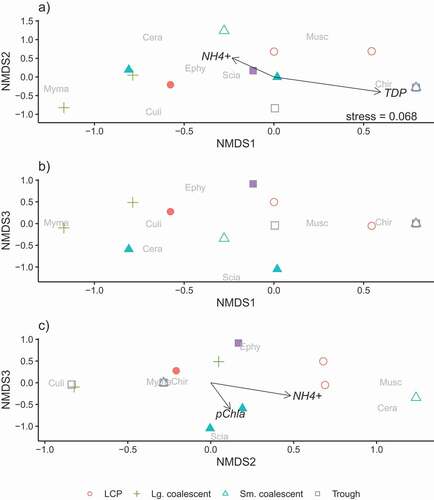
Figure 5. Ordination plots of insect communities emerging from arctic thaw ponds in mid-July. Points represent communities in each of the different pond classes (LCP, small coalescent, large coalescent, and trough) and habitats (open symbols = center and filled symbols = margin) collected over ten days in 2013. Points closer to one another represent communities that are more similar. The proximity of the insect family name to a point indicates greater abundance and association to that pond/habitat. The habitat centroids for pond center (C) and margin (M) are shown when the factor is associated with the emergent insect communities (p < 0.10). Insect families are Brac = Braconidae, Ceci = Cecidomyiidae, Cera = Ceratopogonidae, Chir = Chironomidae, Culi = Culicidae, Ephy = Ephydridae, Ichn = Ichneumonidae, Myma = Mymaridae, and Scia = Sciaridae. Sciaridae and Mymaridae were staggered slightly on the first and third axes (b) to reduce overlap and improve legibility in the figure.

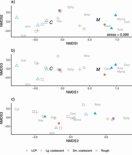
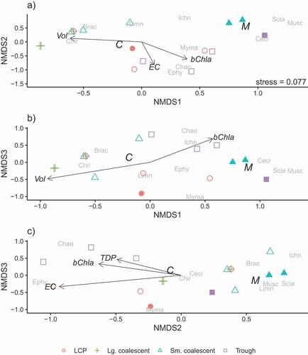
Figure 6. Ordination plots, on three dimensions, of insect communities emerging from arctic thaw ponds in late July. Points represent communities in each of the different pond classes (LCP, small coalescent, large coalescent, and trough) and habitats (open symbols = center and filled symbols = margin) collected over ten days in 2013. Points closer to one another represent communities that are more similar. The proximity of the insect family name to a point indicates greater abundance and association to that pond/habitat. The habitat centroids for pond center (C) and margin (M) are shown when the factor is associated with the emergent insect communities (p < 0.10). The arrows and labels represent the environmental vectors (p < 0.10) associated with the axes of the emergent insect communities. Length of the arrow is related to the strength of the relationship. Insect families are Brac = Braconidae, Ceci = Cecidomyiidae, Chao = Chaoboridae, Chir = Chironomidae, Ephy = Ephydridae, Ichn = Ichneumonidae, Limn = Limnephilidae, Musc = Muscidae, Myma = Mymaridae, and Scia = Sciaridae. Sciaridae and Muscidae were staggered slightly on the first and second axes to reduce overlap and improve legibility in the figure.

Environmental correlates

Associations between environmental variables and the emerging insect community varied across the three time periods in July; these associations were likely driven by the correlations between pond classes and individual variables that change over time (Figure 7; e.g., volume). Period 1 (Figure 4), ordination of insect communities (stress = 0.068) correlated weakly with NH₄⁺ (NMDS1 and 2: R² = 0.498, p = 0.078; NMDS2 and 3: R² = 0.421, p = 0.098), TDP (NMDS1 and 2: R² = 0.393, p = 0.085), and pChla (NMDS2 and 3: R² = 0.375, p = 0.098). The NH₄⁺ gradient was associated with small coalescent, large coalescent, and LCP pond communities containing Ceratopogonidae (Diptera) and Muscidae (Diptera); low values of NH₄⁺ in trough ponds were reflected in community separation (Figures 4a and 4c). The association of TDP to community separation was weakly related with high Chironomidae (Diptera) abundance in three ponds of different classes but separated large coalescent pond communities where TDP was consistently lower (Figure 3a). Lastly, a slight association was found between pChla and small coalescent pond margin communities that included Sciaridae (Figure 4c).

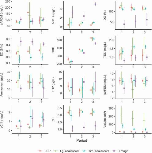
Figure 7. Mean with standard deviation of the ten-day average value for environmental variables during three ten-day time periods collected in July 2013 in each of the pond classes. Variables include bAFDM, bChla, DO, EC, GDD, TDN, NH₄⁺(Ammonium), TDP, pAFDM, pChla, pH, and volume.

In period 2 (Figure 5), only division of pond center and margin habitat contributed to differentiation of pond communities (stress = 0.099). Separation of communities between pond centers and margins was strong along the first axis (NMDS1 and 2: R² = 0.364, p = 0.003; NMDS1 and 3: R² = 0.382, p = 0.012). Margin communities in LCP and small coalescent ponds were associated with abundance of dipteran Ceratopogonidae, Cecidomyiidae, Sciaridae, and Mymaridae. The community in the margin of the trough pond, however, was more similar to those in trough pond centers than to the other margin communities, based on proximity of points in the ordination. No other environmental correlates with pond communities were apparent during this time period.

In period 3, ordination of insect communities (stress = 0.077) indicated strong separation between center and margin habitat, which appeared on each of the three axes (Figure 6; NMDS1 and 2: R² = 0.272, p = 0.015; NMDS1 and 3: R² = 0.318, p = 0.012; NMDS2 and 3: R² = 0.164, p = 0.091). Higher abundances of terrestrial origin insects (e.g., Cecidomyiidae) were associated with margins, whereas those of aquatic origin (e.g., Chironomidae and Limnephilidae [Trichoptera]) were associated with pond centers. The bChla gradient, with higher values in trough ponds relative to other pond classes, was correlated with abundance of Chaoboridae and strongly associated with the first axis and also with the second and third (NMDS1 and 2: R² = 0.535, p = 0.016; NMDS1 and 3: R² = 0.378, p = 0.077; NMDS2 and 3: R² = 0.413, p = 0.063). The EC gradient was strongest along the second axis, with higher values associated with Ephydridae and Chaoboridae in LCP and trough ponds (NMDS1 and 2: R² = 0.690, p = 0.001; NMDS2 and 3: R² = 0.690, p = 0.002). Volume sorted ponds primarily along the first axis (NMDS1 and 2: R² = 0.316, p = 0.076; NMDS1 and 3: R² = 0.317, p = 0.077), with large coalescent ponds, associated with Chironomidae, largely separated from the small-volume trough pond and margin communities (Figures 6a and 6b). Total dissolved phosphorus gradient appeared along the second and third axes, weakly associated with trough ponds and the Chaoboridae found in those communities (Figure 6c; NMDS2 and 3: R² = 0.374, p = 0.062).

Discussion

Summary

In this study, we evaluated emerging insect communities in thaw ponds of varying morphology as a means of determining the availability of insect subsides to arctic terrestrial ecosystems. Overall, the density and timing of total emergence varied little among the different thaw ponds, but the composition of insects varied through time and among the pond classes. The differences in compositional response to pond morphology and their related environmental characteristics suggested that for some insect taxa (e.g., Limnephilidae, Chaoboridae) pond class may be important for production. The strongest driver of composition, however, was the difference between pond margin or center habitat. Insect assemblages were characterized by terrestrial taxa in moist soil margins and aquatic emergent taxa in the wetted centers. Production of different taxa depended on the pond surface area that remained wetted during the growing season relative to the margins that were exposed. As we saw between the dry summer in 2012 and wet summer in 2013, these relative areas are likely to vary among pond classes and years given the high climatic variability in the Arctic and sensitivity of shallow pond water budgets. In addition to changes in pond volume (wetted area), environmental gradients of TDP, NH₄⁺, EC, and bChla and pChla differed among thaw ponds at different periods during the growing season, suggesting that the greatest differences in emerging community composition may be related to these morphology-related drivers.

Emergence phenology

The timing of total insect emergence from arctic thaw ponds did not differ between LCP, small or large coalescent, or trough ponds. Only within small coalescent ponds between years did we find differences in the density of emergence. We speculate that this may have been the result of drought-related water loss in 2012, causing aquatic insects to become concentrated in the available volume of water before emerging. Density of emerging insects was greater in all of the pond classes in 2012, indicating that this may have occurred across all pond classes to varying degrees. Emergence peaked in early July and then rapidly declined to the end of the growing season. Within the bounds of our study period, we failed to capture the ascending limb of the emergence curves from the early season period between thaw and trap deployment (e.g., “absolute spring species”; Danks and Oliver 1972). When sampling ceased in early to mid-August, ponds were still producing more than 300 insects m⁻² d⁻¹ as a subsidy to the terrestrial ecosystem and the end point of emergence remains unknown. The majority of aquatic insect production came from the Chironomidae. Their emergence phenology in the Arctic has been relatively well studied compared to other insect families, and species emergence synchrony has been shown to be important, given the limited opportunity for mating during their brief adult life stage (Danks and Oliver 1972; Butler, Miller, and Mozley 1980; Butler 1982).

We found no evidence of temperature-related differences when comparing timing and density of emerging insects across the pond types. If temperature had played a role in distinguishing phenology among pond classes, then we should have seen reduced or delayed emergence from the cooler trough ponds (Greig et al. 2012; Bolduc et al. 2013; Anderson, Albertson, and Walters 2019) and more insects emerging from warmer ponds like LCPs, where temperatures can reach maximum temperatures around 20°C in June and July (Koch, Gurney, and Wipfli 2014). There was no evidence of emergence reductions or delays in trough ponds or increased emergence in LCPs. This was counter to our expectation and a surprising result, given direct responses to temperature among some arctic insects (Danks and Oliver 1972; Danks 2007) and findings in experimental studies that provide support for links between warmer temperatures and earlier emergence (Harper and Peckarsky 2006; Greig et al. 2012; Sardiña et al. 2017). Deployment of temperature loggers at mid-level depth in the water column likely failed to capture the full range of available thermal habitats in the ponds; for example, sediments may warm to a greater extent (Danks 2007). Additionally, warming from solar radiation on the unshaded loggers may have inadvertently homogenized the temperature readings across shallow, bowl-shaped pond classes (Johnson and Wilby 2013), although we were able to capture relative thermal differences between wedge-shaped trough ponds and the other classes.

Rather than direct temperature effects, some studies found that date of snowmelt was a better predictor of emergence for multiple families, including Chironomidae, Culicidae, Muscidae, and Sciaridae (Høye and Forchhammer 2008; Culler, Ayres, and Virginia 2015), and that in terrestrial habitats, emergence advanced with the growing season (Kwon et al. 2019; Saalfeld et al. 2019). Emergence of terrestrial or semiaquatic taxa may have been a function of cumulative growing degree days in terrestrial habitats (Hodkinson et al. 1996; Bolduc et al. 2013). Information on snowmelt and ice-off date, however, was not collected at each of the study ponds and is only known broadly for the region. Generally, advancement in the phenology of insect prey has led to mismatches between insect peak abundance and shorebird hatch dates (e.g., Reneerkens et al. 2016; Saalfeld et al. 2019). Effects of mismatch, including reduced chick growth, can occur in years of early snowmelt (Saalfeld et al. 2019), when temperature-dependent insects emerge prior to hatch (Høye and Forchhammer 2008; Culler, Ayres, and Virginia 2015). Among some insect taxa, however, prolonged emergence periods or variation in emergence across individual ponds or habitat patches can provide stable food resources for chick growth even when hatch dates fall after peak prey (i.e., insect) abundance (Reneerkens et al. 2016; Leung et al. 2018; Anderson, Albertson, and Walters 2019; Kwon et al. 2019).

Composition and environmental correlates

The analysis of community composition at three sequential time periods allowed us to examine environmental correlates of the community over time, which further helped us describe some of the phenological differences in insect emergence. Mosquitoes (Culicidae, Diptera) and biting midges (Ceratopogonidae, Diptera) were represented in samples collected in early and mid-July. Mosquitoes are known to emerge early, shortly after ice-out (Danks 2007; Culler, Ayres, and Virginia 2015); emergence at the study location was recorded as an abrupt arrival, five days before complete snowmelt on 20 June 2013 (E. Torvinen, University of Alaska Fairbanks, personal communication, March 2, 2020; Uher-Koch, Gurney, and Ruthrauff 2013). The emergence of Limnephilidae and Chaoboridae, conversely, was not evident until late July, indicating a different strategy or cue for emergence timing than used for early emergers like mosquitoes (Danks 2004). Surprisingly, the number of GDD was not correlated with any period of pond community ordination, despite its potential importance (Danks, Kukal, and Ring 1994; Bolduc et al. 2013). Our relatively late temperature logger deployment (on DoY 166), however, may have failed to capture important early season thermal differences and growing degree day estimates later in the season.

We found associations between pond margins and insects of terrestrial origin (e.g., Cecidomyiidae and Sciaridae), particularly at the end of July, when water levels were lowest. The strength of the community association with habitat increased from mid- to late July, indicating the increasing importance of water losses and margin exposure later in the growing season. Early in July, prior to water losses in the ponds, the center/margin habitat factor was not relevant to the separation of pond communities. Terrestrial insects, like Sciaridae, lay their eggs in moist soils (Borror, Triplehorn, and Johnson 1989), which were available seasonally after water levels receded in all pond classes but were prevalent in LCP and small coalescent ponds. Terrestrial insect families that rely on moist soils or riparian plants may emerge from wetland habitats during regular hydroperiod cycles or during drought conditions (e.g., Whiles and Goldowitz 2001; Sim et al. 2013).

In 2012, when climate conditions were dry and more margin was exposed, the proportion of terrestrial insects increased. Therefore, terrestrial or semi-aquatic insect emergence from thaw pond margins may depend on the prevalence of wet sediments, pond morphology, and annual or seasonal variability in evaporative losses and precipitation. Because some insect taxa may take multiple summer seasons to fully develop (Butler, Miller, and Mozley 1980; Danks, Kukal, and Ring 1994), lag effects, or the legacy of seasons past, may affect the emergence composition or environmental associations seen here (Sim et al. 2013). Given the duration of the study and sampling constraints, we were not able to consider these temporal shifts and the associated insect response. Yet, water body permanence is often a key factor driving community composition (Batzer 2013; Sim et al. 2013), and ponds with standing water and moist soil margins can produce diverse assemblages of insects (Butler, Miller, and Mozley 1980; McInerney et al. 2017). Within-pond habitats have been shown to influence the composition, abundance, and phenology of insect fluxes across ecosystem boundaries (Paasivirta, Lahti, and Perätie 1988; Danks, Kukal, and Ring 1994; Greig et al. 2012; Jooste, Samways, and Deacon 2020).

In thermokarst ponds near Utqiaġvik (formerly Barrow, AK), composition within the Chironomidae family varied between pond centers and vegetated margins (Butler, Miller, and Mozley 1980), suggesting that emergent communities at the species level may vary more than we could determine with our family-level analyses. In arctic lakes and streams, sub-family-level Chironomidae composition varies, with different species occupying diverse habitats depending on their environmental tolerance (Hershey 1985; Scott et al. 2011). The association of parasitic wasps (Ichneumonidae and Braconidae) in samples from pond centers was unexpected. These insects are expected in pond margins and among macrophytes where they parasitize or obtain immature hosts, yet little is known about their specific habits (Bennett 2008). There are several possibilities that address their presence, including reemergence of female wasps after they traversed the pond bottom to infect a host, initial emergence of a wasp from their aquatic host, or increased access to damp substrates when minimal water occurred under the traps during the ten- to fourteen-day sampling period.

We found notable differences among the thaw pond communities, including associations of Chaoboridae with trough ponds and Braconidae and Limnephilidae with small coalescent ponds. Experimental studies reveal that there is often a synergistic effect of multiple factors, including nutrients, temperature, and predators, that influence emergence (Harper and Peckarsky 2006; Greig et al. 2012; Culler, Ayres, and Virginia 2015; Jonsson et al. 2015), and differences in resource availability among habitat patches (i.e., pond classes) may limit production of individual macroinvertebrate taxa (Paasivirta, Lahti, and Perätie 1988; Beaty, Fortino, and Hershey 2006; Hornung and Foote 2006). When examined for potential environmental associations, communities were correlated with six different gradients: bChla, pChla, EC, NH₄⁺, TDP, and volume. With the exception of TDP, different variables were relevant in early July compared to late July, with no weak or strong associations found in mid-July. Weak associations with pChla, NH₄⁺, and TDP in early July may indicate variation in early season productivity before uptake by pond biota (Hobbie 1984; Rautio et al. 2011). Earlier work by Koch, Gurney, and Wipfli (2014) found that declines in TDP correlated with increases in pChla in LCP ponds, implying uptake of P by primary producers. In agreement, we found that the communities in LCP ponds were negativity correlated with TDP and positively correlated with pChla.

In late July, the strongest community associations occurred with gradients of EC and bChla, with small coalescent ponds and trough ponds on opposing ends of these gradients. Weak associations with TDP and volume were also evident. These correlations also related to separation of trough pond communities from those in the other classes. High EC in trough ponds results from thawing of the underlying permafrost wedge (Koch, Gurney, and Wipfli 2014), and their connection to the permafrost via mineral-rich, subsurface inflows differentiated these ponds from others. An increasing trend in bChla in trough ponds over the growing season suggests that an early season nutrient influx (see Koch, Gurney, and Wipfli 2014) may have been taken up by benthic primary producers. Trophic interactions and consumption of primary consumers by predaceous Choaboridae may have limited grazing on benthic algae or, potentially, the slow decay of sedimenting algae in cold trough ponds led to relatively higher bChla concentrations (Wauthy and Rautio 2020). Limnephilidae may use warmer, more productive ponds. The association with low values of TDP, which declines over the growing season (see Koch, Gurney, and Wipfli 2014), suggested that P was taken up by the biota. Interestingly, characteristics of these shallow, relatively warm thaw ponds (e.g., early drying) may provide necessary emergence cues to the larvae, including temperature accumulation (Hogg and Williams 1996) or declining water levels and crowding (Lund et al. 2016). Most important, the pond’s morphology, which plays an important role in water budgets, nutrient concentrations, and, potentially, their productivity (Koch, Gurney, and Wipfli 2014), acts indirectly on the biota within.

Conclusions

This study is one of few that examines the role of environmental factors on emergent aquatic insect community composition and phenology in arctic ponds. Our findings indicated that emergent communities differed among some, but not all, classes of thaw ponds, and community dissimilarity was primarily associated with habitat and variables that differed strongly in trough ponds, which may be highly relevant in the future, due to the shifting mosaic of pond types and the increasing prevalence of troughs. Counter to expectations, timing of total insect emergence was not consistently earlier in warmer ponds, although we missed temperature readings and emergence collection for the first days of pond thaw. Extending temporal sampling could provide more detail on the composition and density of early season insect emergence. Our findings indicated that emergence composition varied among families and pond classes, with habitats in the ponds supporting different families of insects. Here, investigation of additional habitat features such as vegetation cover or type or substrate composition (e.g., Beaty, Fortino, and Hershey 2006; Hornung and Foote 2006) would clarify their role in insect distribution in arctic ponds. High levels of unexplained variation are not uncommon among communities of wetland insects, because these organisms are highly adaptable and diverse. Similar to other studies, our results suggest that interactions between insects and their environment are complex and outcomes are difficult to predict (Batzer 2013).

These arctic thaw ponds provided an important energy subsidy to neighboring terrestrial systems in the form of aquatic, semiaquatic, and moist ground insects. The provisions of Chironomidae, which made up greater than 80 percent of the emergent insects, were a reliable and abundant source to the terrestrial ecosystem during the growing season. Emergence of other aquatic insects, including the important Limnephilidae (Cottam 1939; Robertson and Savard 2002), were variable across thaw ponds due to heterogeneity in environmental conditions (Koch, Gurney, and Wipfli 2014), which may affect the emergence of insects at the species level (Harper and Peckarsky 2006; Anderson, Albertson, and Walters 2019). The steady advancement of spring due to warming could advance insect phenology, change composition patterns, or introduce variability in the availability of emerging insects, which may result in phenological mismatches with predators, alter energy flow and food web structure, or change in the recipient population’s density or growth (Sabo and Power 2002; Høye and Forchhammer 2008; Larsen, Muehlbauer, and Marti 2016; Kwon et al. 2019).

Acknowledgments

We thank numerous individuals, notably Laura Garey, Eric Torvinen, Constance Johnson, Mark Gilbertson, Megan Zarzicki, and Chris Gurney for help in the field and long hours counting bugs. We thank Gordon Brower and commissioners of the North Slope Borough Planning and Community Services Department and the North Slope Borough, Department of Wildlife Management for their assistance and feedback on this research. We also thank the members of the NPR-A Subsistence Advisory Panel for their comments on how to best conduct our work in the Arctic to reduce disturbance to wildlife and subsistence activities. We thank the Arctic field office of the Bureau of Land Management for logistical and technical support. Thank you to Wendy Monk for providing comment on an early version of this article. Thanks also to two anonymous reviewers for providing thoughtful feedback.

Disclosure statement

No potential conflict of interest was reported by the authors.

Supplementary material

Supplemental material for this article can be accessed on the publisher’s website.

Additional information

Funding

Funding was provided by the Changing Arctic Ecosystem Initiative supported by the Wildlife program of the USGS Ecosystem Mission Area. Any use of trade, firm, or product names is for descriptive purposes only and does not imply endorsement by the U.S. Government. The authors report no competing interest.

References

- Anderson, H. E., L. K. Albertson, and D. M. Walters. 2019. Thermal variability drives synchronicity of an aquatic insect resource pulse. Ecosphere 10 (8):e02852. doi:https://doi.org/10.1002/ecs2.2852.
- Andresen, C. G., and V. L. Lougheed. 2015. Disappearing Arctic tundra ponds: Fine-scale analysis of surface hydrology in drained thaw lake basins over a 65 year period (1948–2013). Journal of Geophysical Research: Biogeosciences 120:466–79. doi:https://doi.org/10.1002/2014JG002778.
- Batzer, D. P. 2013. The seemingly intractable ecological responses of invertebrates in North American wetlands: A review. Wetlands 33 (1):1–15. doi:https://doi.org/10.1007/s13157-012-0360-2.
- Baxter, C. V., K. D. Fausch, and W. C. Saunders. 2005. Tangled webs: Reciprocal flows of invertebrate prey link streams and riparian zones. Freshwater Biology 50 (2):201–20. doi:https://doi.org/10.1111/j.1365-2427.2004.01328.x.
- Beaty, S. R., K. Fortino, and A. E. Hershey. 2006. Distribution and growth of benthic macroinvertebrates among different patch types of the littoral zone of two arctic lakes. Freshwater Biology 51 (12):2347–61. doi:https://doi.org/10.1111/j.1365-2427.2006.01664.x.
- Bennett, A. M. R. 2008. Aquatic hymenoptera. In An introduction to the aquatic insects of North America, ed. R. W. Merritt, K. W. Cummins, and M. B. Berg, 4th ed., 673–85. Dubuque, IA: Kendall/Hunt Publishing Company.
- Bolduc, E., N. Casajus, P. Legagneux, L. McKinnon, H. G. Gilchrist, M. Leung, J. Bêty, D. Reid, P. A. Smith, and C. M. Buddle. 2013. Terrestrial arthropod abundance and phenology in the Canadian Arctic: Modelling resources availability for Arctic-nesting insectivorous birds. The Canadian Entomologist 145 (2):155–70. doi:https://doi.org/10.4039/tce.2013.4.
- Borror, D. J., C. A. Triplehorn, and N. F. Johnson. 1989. An introduction to the study of insects (No. Ed. 6). Philadelphia, PA: Saunders college publishing.
- Burnham, K. P., and D. R. Anderson. 1998. Practical use of the information-theoretic approach. In Model selection and inference, 75–117. New York, NY: Springer.
- Burpee, B. T., and J. E. Saros. 2020. Cross-ecosystem nutrient subsides in Arctic and alpine lakes: Implications of global change for remote lakes. Environmental Science: Process and Impacts 22:1166–89. doi:https://doi.org/10.1039/c9em00528e.
- Butler, M. G. 1982. A 7-year life cycle for two Chironomus species in arctic Alaskan tundra ponds (Diptera: Chironomidae). Canadian Journal of Zoology 60 (1):58–70. doi:https://doi.org/10.1139/z82-008.
- Butler, M. G., M. C. Miller, and S. Mozley. 1980. Arctic macrobenthos. In Limnology of Tundra Ponds, Barrow, Alaska, ed. J. E. Hobbie, 297–339. Stroudsburg, PA: Dowden, Hutchinson & Ross, Inc.
- CAVM Team. 2003. Circumpolar Arctic vegetation map. (1:7,500,000 scale). Conservation of Arctic Flora and Fauna (CAFF) Map No. 1. Anchorage, Alaska: U.S. Fish and Wildlife Service. ISBN: 0-9767525-0-6, ISBN-13: 978-0-9767525-0-9. https://www.geobotany.uaf.edu/cavm/.
- Cottam, C. 1939. Food habits of North American diving ducks. Vol. 643. Washington, DC: Department of Agriculture.
- Culler, L. E., M. P. Ayres, and R. A. Virginia. 2015. In a warmer Arctic, mosquitoes avoid increased mortality from predators by growing faster. Proceedings of the Royal Society B: Biological Sciences 282:20151549. doi:https://doi.org/10.1098/rspb.2015.1549.
- Cunningham, J. A., D. C. Kesler, and R. B. Lanctot. 2016. Habitat and social factors influence nest-site selection in Arctic-breeding shorebirds. The Auk 133 (3):364–77. doi:https://doi.org/10.1642/AUK-15-196.1.
- Cushman, R. M. 1983. An inexpensive, floating, insect-emergence trap. Bulletin of Environmental Contamination and Toxicology 31(5):547–50.
- Custer, T. W., and F. A. Pitelka. 1978. Seasonal trends in summer diet of the Lapland Longspur near Barrow, Alaska. The Condor 80 (3):295–301. doi:https://doi.org/10.2307/1368039.
- Danks, H. V. 2004. Seasonal adaptations in Arctic insects. Integrative and Comparative Biology 44 (2):85–94. doi:https://doi.org/10.1093/icb/44.2.85.
- Danks, H. V. 2007. How aquatic insects live in cold climates. The Canadian Entomologist 139 (4):443–71. doi:https://doi.org/10.4039/n06-100.
- Danks, H. V., and D. R. Oliver. 1972. Seasonal emergence of some high Arctic Chironomidae (Diptera). The Canadian Entomologist 104 (5):661–86. doi:https://doi.org/10.4039/Ent104661-5.
- Danks, H. V., O. Kukal, and R. A. Ring. 1994. Insect cold-hardiness: Insights from the Arctic. Arctic 47 (4):391–404. doi:https://doi.org/10.14430/arctic1312.
- Greig, H. S., P. Kratina, P. L. Thompson, W. J. Palen, J. S. Richardson, and J. B. Shurin. 2012. Warming, eutrophication, and predator loss amplify subsidies between aquatic and terrestrial ecosystems. Global Change Biology 18 (2):504–14. doi:https://doi.org/10.1111/j.1365-2486.2011.02540.x.
- Gurney, K., and B. Uher-Koch. 2012. Breeding conditions report for Chipp North, USA, 2012. In ARCTIC BIRDS: An international breeding conditions survey (Online database), ed. M. Soloviev and P. Tomkovich. Updated September 20, 2013. Accessed January 6, 2017. http://www.arcticbirds.net/info12/us71us8012.html.
- Harper, M. P., and B. L. Peckarsky. 2006. Emergence cues of a mayfly in a high-altitude stream ecosystem: Potential response to climate change. Ecological Applications 16 (2):612–21. doi:https://doi.org/10.1890/1051-0761(2006)016[0612:ECOAMI]2.0.CO;2.
- Hershey, A. E. 1985. Littoral chironomid communities in an Arctic Alaskan lake. Holarctic Ecology 8:39–48.
- Hobbie, J. E. 1984. The ecology of tundra ponds of the Arctic Coastal Plain: A community profile. FWS/OBS—83/25, US FISH Wildlife Service.
- Hodkinson, I. D., S. J. Coulson, N. R. Webb, W. Block, A. T. Strathdee, J. S. Bale, and M. R. Worland. 1996. Temperature and the biomass of flying midges (Diptera: Chironomidae) in the high Arctic. Oikos 75 (2):241–48. doi:https://doi.org/10.2307/3546247.
- Hogg, I. D., and D. D. Williams. 1996. Response of stream invertebrates to a global-warming thermal regime: an ecosystem level manipulation. Ecology 77(2):395–407.
- Holmes, R. T., and F. A. Pitelka. 1968. Food overlap among coexisting sandpipers on northern Alaskan tundra. Systematic Zoology 17 (3):305–18. doi:https://doi.org/10.2307/2412009.
- Hornung, J. P., and A. L. Foote. 2006. Aquatic invertebrate responses to fish presence and vegetation complexity in western boreal wetlands, with implications for waterbird productivity. Wetlands 26 (1):1–12. doi:https://doi.org/10.1672/0277-5212(2006)26[1:AIRTFP]2.0.CO;2.
- Høye, T. T., and M. C. Forchhammer. 2008. Phenology of high-Arctic arthropods: Effects of climate on spatial, seasonal, and inter-annual variation. Advances in Ecological Research 40:299–324.
- Iwata, T., S. Nakano, and M. Murakami. 2003. Stream meanders increase insectivorous bird abundance in riparian deciduous forests. Ecography 26(3):629–37.
- Johnson, M. F., and R. L. Wilby. 2013. Shield or not to shield: Effects of solar radiation on temperature sensor accuracy. Water 5 (4):1622–37. doi:https://doi.org/10.3390/w5041622.
- Jonsson, M., P. Hedström, K. Stenroth, E. R. Hotchkiss, F. R. Vasconcelos, J. Karlsson, and P. Byström. 2015. Climate change modifies the size structure of assemblages of emerging aquatic insects. Freshwater Biology 60 (1):78–88. doi:https://doi.org/10.1111/fwb.12468.
- Jooste, M. L., M. J. Samways, and C. Deacon. 2020. Fluctuating pond water levels and aquatic insect persistence in a drought-prone Mediterranean-type climate. Hydrobiologia 847 (5):1315–26. doi:https://doi.org/10.1007/s10750-020-04186-1.
- Jorgenson, M. T., M. Kanevskiy, Y. Shur, N. Moskalenko, D. R. N. Brown, K. P. Wickland,R. Striegl, and J. C. Koch. 2015. Role of ground ice dynamics and ecological feedbacks in recent ice wedge degradation and stabilization. Journal of Geophysical Research: Earth Surface 300–16. doi:https://doi.org/10.1002/2015JF003602.
- Jorgenson, M. T., and Y. Shur. 2007. Evolution of lakes and basins in northern Alaska and discussion of the thaw lake cycle. Journal of Geophysical Research 112 (F2):F02S17. doi:https://doi.org/10.1029/2006JF000531.
- Koch, J. C., K. Gurney, and M. Wipfli. 2014. Morphology‐dependent water budgets and nutrient fluxes in Arctic thaw ponds. Permafrost and Periglacial Processes 25 (2):79–93. doi:https://doi.org/10.1002/ppp.1804.
- Koch, J. C., K. E. Gurney, M. S. Wipfli, and J. A. Schmutz. 2019. Physical, chemical, and invertebrate data from Chipp North pond manipulations, North Slope, Alaska, 2013: U.S. Geological Survey data release. doi:https://doi.org/10.5066/P9K5EV4N.
- Koch, J. C., M. T. Jorgenson, K. P. Wickland, M. Kanevskiy, and R. Striegl. 2018. Ice wedge degradation and stabilization impact water budgets and nutrient cycling in Arctic trough ponds. Journal of Geophysical Research: Biogeosciences 123 (8):2604–16. doi:https://doi.org/10.1029/2018JG004528.
- Kwon, E., E. L. Weiser, R. B. Lanctot, S. C. Brown, H. R. Gates, G. Gilchrist, and B. K. Sandercock. 2019. Geographic variation in the intensity of warming and phenological mismatch between Arctic shorebirds and invertebrates. Ecological Monographs 84 (4):e01383.
- Larsen, S., J. D. Muehlbauer, and E. Marti. 2016. Resource subsidies between stream and terrestrial ecosystems under global change. Global Change Biology 22 (7):2489–504. doi:https://doi.org/10.1111/gcb.13182.
- Laske, S. M., and K. E. B. Gurney. 2021. Insect emergence from Arctic Coastal Plain thaw ponds, 2012–2013: U.S. Geological Survey data release. doi:https://doi.org/10.5066/P9FG9DEO.
- Leung, M. C.-Y., E. Bolduc, F. I. Doyle, D. G. Reid, B. S. Gilbert, A. J. Kenney, C. J. Krebs, and J. Bêty. 2018. Phenology of hatching and food in low Arctic passerines and shorebirds: Is there a mismatch? Arctic Science 4 (4):538–56. doi:https://doi.org/10.1139/as-2017-0054.
- Liljedahl, A. K., J. Boike, R. P. Daanen, A. N. Fedorov, G. V. Frost, G. Grosse, M. Necsoiu, Y. Iijma, J. C. Jorgenson, and N. Matveyeva. 2016. Pan-Arctic ice-wedge degradation in warming permafrost and its influence on tundra hydrology. Nature Geoscience 9 (4):312–18. doi:https://doi.org/10.1038/ngeo2674.
- Loskutova, O. A. 2020. Benthic invertebrate communities of lakes in the Polar Ural Mountains (Russia). Polar Biology 43 (6):755–66. doi:https://doi.org/10.1007/s00300-020-02677-4.
- Lund, J. O., S. A. Wissinger, and B. L. Peckarsky. 2016. Caddisfly behavioral responses to drying cues in temporary ponds: Implications for effects of climate change. Freshwater Science 35(2):619–630.
- Marczak, L. B., R. M. Thompson, and J. S. Richardson. 2007. Meta-analysis: Trophic level, habitat, and productivity shape the food web effects of resource subsidies. Ecology 88 (1):140–48. doi:https://doi.org/10.1890/0012-9658(2007)88[140:MTLHAP]2.0.CO;2.
- McInerney, P. J., R. J. Stoffels, M. E. Shackleton, and C. D. Davey. 2017. Flooding drives a macroinvertebrate biomass boom in ephemeral floodplain wetlands. Freshwater Science 36 (4):726–38. doi:https://doi.org/10.1086/694905.
- Merritt, R. W., K. W. Cummins, and M. B. Berg. 2008. An introduction to the aquatic insects of North America (No. Ed. 4). Dubuque, IA: Kendall/Hunt Publishing Company.
- Nakano, S., and M. Murakami. 2001. Reciprocal subsides: Dynamic interdependence between terrestrial and aquatic food webs. Proceedings of the National Academy of Sciences 98 (1):166–70. doi:https://doi.org/10.1073/pnas.98.1.166.
- Oksanen, J., F. G. Blanchet, M. Friendly, R. Kindt, P. Legendre, D. McGlinn, P. R. Minchin, R. B. O’Hara, G. L. Simpson, P. Solymos, et al. 2019. Vegan: Community ecology package. R package version 2.5-5. https://CRAN.R-project.org/package=vegan.
- Paasivirta, L., T. Lahti, and T. Perätie. 1988. Emergence phenology and ecology of aquatic and semi-terrestrial insects on a boreal raised bog in Central Finland. Holarctic Ecology 11 (2):96–105.
- Pedersen, E. J., D. L. Miller, G. L. Simpson, and N. Ross. 2019. Hierarchical generalized additive models in ecology: An introduction with mgcv. PeerJ 7:e6876. doi:https://doi.org/10.7717/peerj.6876.
- Rautio, M., F. Dufresne, I. Laurion, S. Bonilla, W. F. Vincent, and K. S. Christoffersen. 2011. Shallow freshwater ecosystems of the circumpolar Arctic. Ecoscience 18 (3):204–22. doi:https://doi.org/10.2980/18-3-3463.
- Reneerkens, J., N. M. Schmidt, O. Gilg, J. Hansen, L. H. Hansen, J. Moreau, and T. Piersma. 2016. Effects of food abundance and early clutch predation on reproductive timing in a high Arctic shorebird exposed to advancements in arthropod abundance. Ecology and Evolution 6 (20):7375–86. doi:https://doi.org/10.1002/ece3.2361.
- Robertson, G. J., and J. L. Savard. 2002. Long-tailed duck (Clangula hyemalis), version 2.0. In The birds of North America, ed. A. F. Poole and F. B. Gill, Ithaca, NY, USA: Cornell Lab of Ornithology. doi:https://doi.org/10.2173/bna.651.
- Saalfeld, S. T., D. C. McEwen, D. C. Kesler, M. G. Butler, J. A. Cunningham, A. C. Doll, R. B. Lanctot, D. E. Gerik, K. Grond, and P. Herzog. 2019. Phenological mismatch in Arctic-breeding shorebirds: Impact of snowmelt and unpredictable weather conditions on food availability and chick growth. Ecology and Evolution 9 (11):6693–707. doi:https://doi.org/10.1002/ece3.5248.
- Sabo, J. L., and M. E. Power. 2002. River-watershed exchange: Effects of riverine subsidies on riparian lizards and their terrestrial prey. Ecology 83 (7):1860. doi:https://doi.org/10.2307/3071770.
- Sardiña, P., J. Beardall, J. Beringer, M. Grace, and R. M. Thompson. 2017. Consequences of altered temperature regimes for emerging freshwater invertebrates. Aquatic Sciences 79 (2):265–76. doi:https://doi.org/10.1007/s00027-016-0495-y.
- Schekkerman, H., I. Tulp, T. Piersma, and G. H. Visser. 2003. Mechanisms promoting higher growth rate in arctic than in temperate shorebirds. Ecophysiology 134:332–42.
- Schriever, T. A., M. W. Cadotte, and D. D. Williams. 2014. How hydroperiod and species richness affect the balance of resource flows across aquatic-terrestrial habitats. Aquatic Sciences 76 (1):131–43. doi:https://doi.org/10.1007/s00027-013-0320-9.
- Scott, R. W., D. R. Barton, M. S. Evans, and J. J. Kaeting. 2011. Latitudinal gradients and local control of aquatic insect richness in a large river system in northern Canada. Journal of the North American Benthological Society 30 (3):621–34. doi:https://doi.org/10.1899/10-112.1.
- Sim, L. L., J. A. Davis, K. Strehlow, M. McGuire, K. M. Trayler, S. Wild, J. Papas, and J. O’Connor. 2013. The influence of changing hydroregime on the invertebrate communities of temporary seasonal wetlands. Freshwater Science 32 (1):327–42. doi:https://doi.org/10.1899/12-024.1.
- Stanley, D. W., and R. J. Daley. 1976. Environmental control of primary productivity in Alaskan Tundra ponds. Ecology 57 (5):1025–33. doi:https://doi.org/10.2307/1941067.
- Uher-Koch, B., K. Gurney, and D. R. Ruthrauff (2013). Breeding conditions report for Chipp North, USA, 2013. ARCTIC BIRDS: An international breeding conditions survey. (Online database), eds. M. Soloviev and P. Tomkovich. Updated August 22, 2015; Accessed March 2, 2020. http://www.arcticbirds.net/info13/us78us8013.html.
- Urban, F. E., and G. D. Clow. 2016. Air temperature, wind speed, and wind direction in the National Petroleum Reserve – Alaska and the Arctic National Wildlife Refuge, 1998-2014. US Geological Survey Open-File Report 2016.
- Wauthy, M., and M. Rautio. 2020. Emergence of steeply stratified permafrost thaw ponds changes zooplankton ecology in subarctic freshwaters. Arctic, Antarctic, and Alpine Research 52 (1):177–90. doi:https://doi.org/10.1080/15230430.2020.1753412.
- Whiles, M. R., and B. S. Goldowitz. 2001. Hydrologic influences on insect emergence production from central Platte River wetlands. Ecological Applications 11 (6):1829–42. doi:https://doi.org/10.1890/1051-0761(2001)011[1829:HIOIEP]2.0.CO;2.
- Woo, M. K., and K. L. Young. 2006. High Arctic wetlands: Their occurrence, hydrological characteristics and sustainability. Journal of Hydrology 320 (3–4):432–50. doi:https://doi.org/10.1016/j.jhydrol.2005.07.025.
- Wood, S. 2017. Generalized additive models. New York: Chapman and Hall/CRC. doi:https://doi.org/10.1201/9781315370279.