Twentieth century warming reflected by the Malan Glacier borehole temperatures, northern Tibetan Plateau

ABSTRACT

The Tibetan Plateau is a high-elevation area in Asia and contains the largest volumes of glaciers outside the polar regions. Reconstruction of the glacier surface temperature history in this area is crucial for better understanding of the process of climate change in the Tibetan Plateau. The Tikhonov regularization method has been used on borehole temperatures measured at Malan Glacier, located on the north Tibetan Plateau, to reconstruct the surface temperature history in the twentieth century. We found that the glacier surface temperature, which rose significantly after the 1960s, increased about 1.1°C over the last century. The warmest period occurred in the 1980s to the 1990s and the highest temperature variation could be 1.5°C to 1.6°C. The results were also compared with those of nearby instrumental temperatures by Wudaoliang meteorological station and the stable oxygen isotope (${\delta }^{18}O$) from the Malan ice core.

KEYWORDS:

• Glacier borehole temperatures
• heat conduction
• Tikhonov regularization method

Introduction

Borehole paleothermometry, a reconstruction of the past ground surface temperature change from subsurface temperatures, is an important tool for understanding climate responses to conditions of a certain area in the past (Muto et al. 2011). The recognition that past climate changes influence the ground surface temperatures, penetrate in the subsurface, and could be recovered from the temperature–depth (T–z) profiles measured at boreholes dates back to Lane (1923). Hotchkiss and Ingersoll (1934) were the first to attempt and infer the timing of the last deglaciation from geothermal data. Interest in borehole temperatures as a record of climate change among the scientific community was aroused by Lachenbruch and Marshall (1986), who suggested that the warming reconstructed from borehole temperatures in permafrost on Alaska’s north coast could be an early sign of the enhanced greenhouse effect predicted by general circulation models (Beltrami and Mareschal 1995). In general, the underground temperature distribution is mainly determined by two types of processes: surface temperature change and heat flux. Temperature changes at the surface slowly propagate downward so that the ground surface temperature history is recorded in the subsurface. Surface warming manifests itself as a positive disturbance in the subsurface; cooling shows up as a negative disturbance. By solving the ordinary heat conduction equation with appropriate initial and boundary conditions, these disturbances can be recollected from T–z profiles measured in boreholes (Louise and Vladimir 2007). Because of firnification and ice flow, the climate reconstruction from T–z profiles for glaciers is more difficult than for other places such as permafrost (Nicholls and Paren 1993). The temperatures down through the ice depend on the heat flux, the ice flow pattern, the past surface temperatures, and accumulation rates. A coupled heat flow equation and inversion algorithm for the reconstruction have become one of the important topics in the field of borehole paleothermometry (Dahl-Jensen and Johnsen 1986; Macayeal, Firestone, and Waddington 1991; Nagornov et al. 2001).

The first attempt to infer past glacier surface temperature (GST) change from the measured T–z profile dates back to Dahl-Jensen and Johnsen (1986) based on the temperature distribution through the Greenland ice sheet at the Dye-3 borehole. Macayeal, Firestone, and Waddington (1991) used control methods and a simple one-dimensional heat equation at Dye-3 to infer past GST change once again. More studies were then undertaken to investigate GST histories in polar regions.A Monte Carlo inverse method has been used on the T–z profiles measured down through the Greenland Ice Core Project borehole, at the summit of the Greenland ice sheet, and the ice borehole near the summit of Law Dome, Antarctica. The results were a 50,000-year temperature history at Greenland Ice Core Project borehole and a 4,000-year history at the summit of Law Dome (Dahl-Jensen et al. 1998; Dahl-Jensen, Morgan, and Elcheikh 1999). At present the history of climatic change has been reconstructed on different timescales worlwide since the Last Glacial Maximum. For instance, the reconstructed result based on the temperature distribution at the ice divide on the Lomonosovfonna plateau (Svalbard) showed that the temperature increased 2°C to 2.5°C in the twentieth century (van de Wal et al. 2002). By means of the algorithm of finite difference inversion, the reconstructions were made for two arctic ice caps (Austfonna and Akademii Nauk), showing that the surface temperature variations of the two ice caps exceeded the average arctic temperature anomalies over the last 150 years by 6°C to 7°C (Nagornov, Konovalov, and Tchijov 2006). Moreover, the analyses of borehole temperatures obtained from East Antarctica and West Antarctica all revealed the warming trend in the twentieth century (Barrett et al. 2009; Muto et al. 2011; Zagorodnov et al. 2012; J. W. Yang et al. 2018). In addition, the analysis of cold glacier borehole temperatures at Illimani, a high-elevation tropical site in Bolivia, showed a temperature rise over the twentieth century (Gilbert et al. 2010). Less research has been done on the reconstruction of paleoclimate by cold glacier borehole temperatures for the low- and middle-latitude regions, and strengthening the study in these areas can help to reveal the climate change at mid-low latitudes with high altitude.

The common merits of this method are that it is based on a simple physical theory, that the past GST conditions can be derived directly from measured T–z profiles and do not need any additional calibration. As the GST signal propagates downward, it is delayed in time and its amplitude decreases exponentially with depth due to the diffusive process of heat conduction. Thus, the ice selectively filters out high-frequency components of the GST oscillations, and the deeper we go, the more the distant past can be inverted (and, unfortunately, becoming more diffused and less credible). This technique is essentially multidecadal and cannot provide information about annual temperature changes or for times near the present. Leading scientists gave an extremely positive evaluation of this method (Broecker 2001). At least for timescales greater than a century or two, only two proxies can yield temperatures that are accurate to 0.5°C: the reconstruction of temperatures from the elevation of mountain snowlines and borehole thermometry. One could declare that at present borehole thermometry undoubtedly represents an independent well-developed research tool in paleoclimatic studies and is an important supplement to climate reconstruction by proxy indicators (Louise and Vladimir 2007).

The Tibetan Plateau (TP) is a high-elevation area in Asia containing the largest volumes of glaciers outside the polar regions and is highly sensitive to climate change (Yao et al. 2019). Meteorological data indicated that the warming rate for the TP was two times of that observed globally in the past fifty years (Chen et al. 2015). Previous temperature reconstructions on the TP were mainly based on proxy data like tree rings or the stable oxygen isotope (${\delta }^{18}O$) in ice cores, and no research has been done on climate reconstruction by glacier borehole temperatures in this area (Bräuning and Mantwill 2004; B. Yang et al. 2009). To better understand the temperature variation of the northern TP during the twentieth century, we present a GST history of borehole paleothermometry analysis at Malan Glacier using the Tikhonov regularization method (Nagornov et al. 2017). The results were also compared with those of nearby instrumental temperatures by Wudaoliang meteorological station and the stable oxygen isotope (${\delta }^{18}O$) from the Malan ice core.

Methods

A heat flow model

The T–z profile measured in the ice borehole $\chi \left(z\right)$, where $z$ is vertical coordinate, can be expressed by the steady-state T–z profile $U\left(z\right)$ that is subjected to long-time geological processes and the temperature perturbation $\theta \left(z\right)$ caused by the GST changes. Thus, the following one-dimensional inverse problem for the heat conduction equation with initial and boundary conditions has to be solved to determine the past GST changes over a period of time $\left[0,t_f\right]$ (Nagornov et al. 2017):

(1) $\left\{\begin{array}{c}\frac{\mathrm{\partial }T}{\mathrm{\partial }t}+w\left(z\right)\frac{\mathrm{\partial }T}{\mathrm{\partial }z}=\kappa \frac{\mathrm{\partial }}{\mathrm{\partial }z}\left(\frac{\mathrm{\partial }T}{\mathrm{\partial }z}\right)\\ \\ T\left(0,t\right)=\mu \left(t\right)\\ \\ \frac{\mathrm{\partial }T}{\mathrm{\partial }z}\left(H,t\right)=0\\ \\ T\left(z,0\right)=0\\ \\ T\left(z,t_f\right)=\theta \left(z\right)\end{array}\right.$(1)

where time $t_f$ corresponds to the end of the period; time $0$ corresponds to the initial time;$T\left(z,t\right)$ is the temperature variation at a certain depth $z$ at time $t$; $w\left(z\right)$ is the vertical velocity of glacier layers; $\kappa$ is the thermal diffusivity; $\mu \left(t\right)$ is the temperature variation on the glacier surface in time from the moment $t=0\left(\mu \left(0\right)=0\right)$ to the time of measurements of the T–z profile $t_f$; and $H$ is the ice thickness.

Solutions of the established model are calculated with the following assumptions: (1) The problem is assumed to be one-dimensional. The horizontal velocity, the horizontal derivatives of $T$, and the internal heat production are negligible. (2) The ice thickness has remained constant in time. (3) Vertical velocity at the surface is assumed to balance the mean accumulation rate and to decline linearly with depth to zero at the base. (4) For the constant thermal conductivity of the subsurface ice, temperature increases steadily with depth. An initial steady-state T–z profile is calculated for present conditions; that is, using the present surface temperature and the bedrock temperature to yield $U\left(z\right)$.

Study area and borehole temperatures

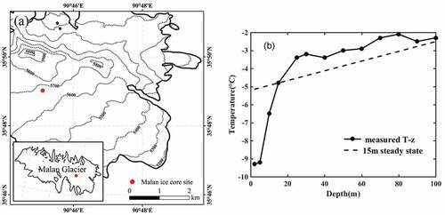
Malan Glacier (35°46′~35°55′N, 90°32′~90°54′E), a large extreme continental glacier with a total area of 195 km² and a summit elevation 6,056 m.a.s.l., is located in Hoh Xil region in the center of the TP. Its equilibrium line altitude varies from 5,430 m.a.s.l. to 5,540 m.a.s.l. (Pu, Yao, and Wang 2001). Since the Little Ice Age the glacier has shown a tendency of shrinking within a very narrow range, which satisfies the assumption that the glacier is in a stable state. Because there is little precipitation in the region in the cold season, the basic feature of the climate is cold and dry with less snow cover. This environment is similar to that of the Coastal Antarctic Ice Sheet (Xie et al. 2000). In May 1999, a 102-m ice core (35°48.4′ N, 90°45.3′ E) was successfully drilled at 5,680 m.a.s.l. (Figure 1a), not reaching the bedrock (Wang et al. 2003). It was not far from the ice divide and the borehole temperatures were measured twice with a precision of 0.01°C, and the logging interval was 5 m for the upper 15 m and 10 m down to 100 m (Figure 1b). The temperature at 15 m was about −4.8°C. By calculation, the ice thickness at the drilling location was 130 m and the bedrock temperature was below the melting point (−1.7°C), indicating that there was no basal melting. The accumulation rate was estimated as 0.23 m a⁻¹ in the last twenty years (Wang et al. 2006). The calculated steady-state T–z profile deviated considerably from the observed profile, indicating that the temperature distribution in the borehole was far from a steady-state distribution (Figure 1b). Under these conditions, the Malan Glacier was a perfect site to study the borehole climatology.

Figure 1. (a) Location map. The Malan Glacier on the Tibetan Plateau showing the ice core site. The glacier outlines were delineated manually using Landsat TM data from 1999, in conjunction with digital elevation model data from 2000 (USGS 2021). (b) The Malan Glacier borehole temperatures (dots) measured in 1999 and the steady state calculated at the annual influence depth of 15 m (dashed)

In Equations (1(1) $\left\{\begin{array}{c}\frac{\mathrm{\partial }T}{\mathrm{\partial }t}+w\left(z\right)\frac{\mathrm{\partial }T}{\mathrm{\partial }z}=\kappa \frac{\mathrm{\partial }}{\mathrm{\partial }z}\left(\frac{\mathrm{\partial }T}{\mathrm{\partial }z}\right)\\ \\ T\left(0,t\right)=\mu \left(t\right)\\ \\ \frac{\mathrm{\partial }T}{\mathrm{\partial }z}\left(H,t\right)=0\\ \\ T\left(z,0\right)=0\\ \\ T\left(z,t_f\right)=\theta \left(z\right)\end{array}\right.$(1) ), the vertical velocity $w\left(z\right)$ was 0.23 m at the glacier surface, which decreased linearly to zero at the base, balancing the accumulation rate (Zagorodnov et al. 2012). The thermal diffusivity $\kappa$ = 1.4 $\times$ 10⁻⁶ m² s⁻¹ (Macayeal, Firestone, and Waddington 1991) and we recovered $\mu \left(t\right)$ for 150 years with a time interval of one year. The calculations were started so far back in time that it was beyond the memory of the system. Equations (1)(1) $\left\{\begin{array}{c}\frac{\mathrm{\partial }T}{\mathrm{\partial }t}+w\left(z\right)\frac{\mathrm{\partial }T}{\mathrm{\partial }z}=\kappa \frac{\mathrm{\partial }}{\mathrm{\partial }z}\left(\frac{\mathrm{\partial }T}{\mathrm{\partial }z}\right)\\ \\ T\left(0,t\right)=\mu \left(t\right)\\ \\ \frac{\mathrm{\partial }T}{\mathrm{\partial }z}\left(H,t\right)=0\\ \\ T\left(z,0\right)=0\\ \\ T\left(z,t_f\right)=\theta \left(z\right)\end{array}\right.$(1) were solved by a Crank-Nicholson finite difference scheme.

Annual influence depth

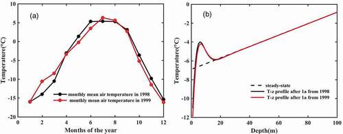
The T–z profile for the upper several meters is affected by seasonal GST change. It is important to determine the depth at which yearly temperature oscillations die away (<0.1°C) because it may have a significant impact on the steady state. Because the borehole was drilled in May 1999, we used data on monthly mean air temperature collected by the nearest Wudaoliang meteorological station (35.13° N, 93.05° E, 4,612.2 m.a.s.l.) in 1998 and 1999 (Figure 2a) as the input conditions to determine the possible annual influence depths. The data were obtained from the China Meteorological Data Service Center (CMDSC 2021). Supposing that the steady-state T–z profile was obtained through linear fitting to the T–z curve in Figure 1b, we inputted initial conditions in the borders to solve Equations (1)(1) $\left\{\begin{array}{c}\frac{\mathrm{\partial }T}{\mathrm{\partial }t}+w\left(z\right)\frac{\mathrm{\partial }T}{\mathrm{\partial }z}=\kappa \frac{\mathrm{\partial }}{\mathrm{\partial }z}\left(\frac{\mathrm{\partial }T}{\mathrm{\partial }z}\right)\\ \\ T\left(0,t\right)=\mu \left(t\right)\\ \\ \frac{\mathrm{\partial }T}{\mathrm{\partial }z}\left(H,t\right)=0\\ \\ T\left(z,0\right)=0\\ \\ T\left(z,t_f\right)=\theta \left(z\right)\end{array}\right.$(1) and possible annual influence depths were obtained. The results showed that yearly temperature oscillations died away at 15 m in both cases (Figure 2b), and 15 m was selected as the annual influence depth for final reconstruction. Therefore, the temperature at 15 m was used to obtain the steady-state T–z profile $U\left(z\right)$ (Figure 1b).

Figure 2. (a) Monthly mean air temperature at Wudaoliang meteorological station in 1998 (black dots) and 1999 (red dots). (b) T–z profiles for the steady state (dashed) and the yearly temperature oscillations using monthly mean air temperature data from 1998 (black line) and 1999 (red line). The 15-m-deep temperature oscillations were 0.05°C in 1998 and 0.09°C in 1999, and both were less than 0.1°C

The Tikhonov regularization method

The Tikhonov regularization method is the determination of $\mu \left(t\right)$ in Equations (1)(1) $\left\{\begin{array}{c}\frac{\mathrm{\partial }T}{\mathrm{\partial }t}+w\left(z\right)\frac{\mathrm{\partial }T}{\mathrm{\partial }z}=\kappa \frac{\mathrm{\partial }}{\mathrm{\partial }z}\left(\frac{\mathrm{\partial }T}{\mathrm{\partial }z}\right)\\ \\ T\left(0,t\right)=\mu \left(t\right)\\ \\ \frac{\mathrm{\partial }T}{\mathrm{\partial }z}\left(H,t\right)=0\\ \\ T\left(z,0\right)=0\\ \\ T\left(z,t_f\right)=\theta \left(z\right)\end{array}\right.$(1) minimizing a smoothing functional consisting of the difference and stabilizer (Zagorodnov, Nagornov, and Thompson 2006; Nagornov et al. 2017):

(2) $\mathrm{\Psi }=\frac{1}{2}{\int }_0^H{\left[R\left\{\mu \left(t\right)\right\}-\theta \left(z\right)\right]}^{2}dz+\alpha \mathrm{\Omega }\left\{\mu \left(t\right)\right\}$(2)

where $R\left\{\mu \left(t\right)\right\}$ is the solution of the direct problem specified by Equations (1)(1) $\left\{\begin{array}{c}\frac{\mathrm{\partial }T}{\mathrm{\partial }t}+w\left(z\right)\frac{\mathrm{\partial }T}{\mathrm{\partial }z}=\kappa \frac{\mathrm{\partial }}{\mathrm{\partial }z}\left(\frac{\mathrm{\partial }T}{\mathrm{\partial }z}\right)\\ \\ T\left(0,t\right)=\mu \left(t\right)\\ \\ \frac{\mathrm{\partial }T}{\mathrm{\partial }z}\left(H,t\right)=0\\ \\ T\left(z,0\right)=0\\ \\ T\left(z,t_f\right)=\theta \left(z\right)\end{array}\right.$(1) without the redetermination condition for temperature variations $\mu \left(t\right)$. $\alpha$ is the regularization parameter matched with the accuracy of the input data and controls the accuracy and stability of the solution. The additional function $\mathrm{\Omega }\left\{\mu \left(t\right)\right\}$ is called the stabilizing function or stabilizer and is related to the smoothness of the solution:

(3) $\mathrm{\Omega }\left\{\mu \left(t\right)\right\}={\int }_0^{t_f}\left[{\mu }^2\left(t\right)+{\left(\frac{d\mu \left(t\right)}{dt}\right)}^2\right]dt$(3)

Minimization of $\mathrm{\Psi }$ can be performed by the gradient method, which is an iteration procedure. It is carried out until the functional $\mathrm{\Psi }$ reaches the minimum with a given accuracy (0.00001), corresponding to the optimal solution of the inverse problem. Let us write $\mu \left(t\right)$ in the form of a finite set of the Fourier series:

(4) $\mu \left(t\right)=\frac{a_0}{2}+\sum _{m=1}^M{a}_{m}cos\left(\frac{2\pi mt}{t_f}\right)+b_{m}sin\left(\frac{2\pi mt}{t_f}\right)$(4)

The initial Fourier coefficients are given in the first iteration step $a_0=a_1=b_1=1$ and the next nth iterations are determined by the following equations:

(5) $a_0^{n+1}=a_0^n-{\gamma }^n\frac{\mathrm{\partial }{\mathrm{\Psi }}^n}{\mathrm{\partial }{a}_0^n},a_m^{n+1}=a_m^n-{\gamma }^n\frac{\mathrm{\partial }{\mathrm{\Psi }}^n}{\mathrm{\partial }{a}_m^n},b_m^{n+1}=b_m^n-{\gamma }^n\frac{\mathrm{\partial }{\mathrm{\Psi }}^n}{\mathrm{\partial }{b}_m^n},m=1,2,\cdots M$(5)

where ${\gamma }^n=0.01$ is the gradient step. The derivatives of the functional in Equation (5)(5) $a_0^{n+1}=a_0^n-{\gamma }^n\frac{\mathrm{\partial }{\mathrm{\Psi }}^n}{\mathrm{\partial }{a}_0^n},a_m^{n+1}=a_m^n-{\gamma }^n\frac{\mathrm{\partial }{\mathrm{\Psi }}^n}{\mathrm{\partial }{a}_m^n},b_m^{n+1}=b_m^n-{\gamma }^n\frac{\mathrm{\partial }{\mathrm{\Psi }}^n}{\mathrm{\partial }{b}_m^n},m=1,2,\cdots M$(5) with respect to the corresponding Fourier coefficients are given by the expressions:

$\begin{array}{rl}& \frac{\mathrm{\partial }{\mathrm{\Psi }}^n}{\mathrm{\partial }{a}_0^n}={\int }_0^H{W}_{a_0}\left(z\right)\left[R\left\{{\mu }^n\left(t\right)\right\}-\theta \left(z\right)\right]dz+\alpha \frac{\mathrm{\partial }{\mathrm{\Omega }}^n}{\mathrm{\partial }{a}_0^n},\hspace{0.17em}\\ & \hspace{0.17em}\frac{\mathrm{\partial }{\mathrm{\Psi }}^n}{\mathrm{\partial }{a}_m^n}={\int }_0^H{W}_{a_m}\left(z\right)\left[R\left\{{\mu }^n\left(t\right)\right\}-\theta \left(z\right)\right]dz+\alpha \frac{\mathrm{\partial }{\mathrm{\Omega }}^n}{\mathrm{\partial }{a}_m^n},\end{array}$

$\begin{array}{rl}& \frac{\mathrm{\partial }{\mathrm{\Psi }}^n}{\mathrm{\partial }{b}_m^n}={\int }_0^H{W}_{b_m}\left(z\right)\left[R\left\{{\mu }^n\left(t\right)\right\}-\theta \left(z\right)\right]dz+\alpha \frac{\mathrm{\partial }{\mathrm{\Omega }}^n}{\mathrm{\partial }{b}_m^n},\\ & m=1,2,\cdots M.\end{array}$(6)

The profiles $W_{a_0}\left(z\right)$, $W_{a_m}\left(z\right)$, and $W_{b_m}\left(z\right)$ are the solutions of the direct problem with the boundary conditions $\mu \left(t\right)=0.5$, $\mu \left(t\right)=cos\left(2\pi t/T_m\right)$, and $\mu \left(t\right)=sin\left(2\pi t/T_m\right)$, respectively. It is easy to show that the term with the stabilizer in Equation (2)(2) $\mathrm{\Psi }=\frac{1}{2}{\int }_0^H{\left[R\left\{\mu \left(t\right)\right\}-\theta \left(z\right)\right]}^{2}dz+\alpha \mathrm{\Omega }\left\{\mu \left(t\right)\right\}$(2) has the form

$\alpha \mathrm{\Omega }={\alpha }_0\frac{a_0^2}{2}+\sum _{m=1}^M\left(a_m^2+b_m^2\right){\xi }_m,$

where ${\xi }_m={\alpha }_0+{\alpha }_1{\left(2\pi /T_m\right)}^2$, ${\alpha }_i=\alpha t_f/2,$ $i=0,1$. In this case,

(7) $\alpha \frac{\mathrm{\partial }{\mathrm{\Omega }}^n}{\mathrm{\partial }{a}_0^n}={\alpha }_0{a}_0^n,\alpha \frac{\mathrm{\partial }{\mathrm{\Omega }}^n}{\mathrm{\partial }{a}_m^n}=2a_m^n{\xi }_m,\alpha \frac{\mathrm{\partial }{\mathrm{\Omega }}^n}{\mathrm{\partial }{b}_m^n}=2b_m^n{\xi }_m$(7)

Thus, to determine the Fourier coefficients given by Equation (4)(4) $\mu \left(t\right)=\frac{a_0}{2}+\sum _{m=1}^M{a}_{m}cos\left(\frac{2\pi mt}{t_f}\right)+b_{m}sin\left(\frac{2\pi mt}{t_f}\right)$(4) , the iteration procedure specified by Equation (5)(5) $a_0^{n+1}=a_0^n-{\gamma }^n\frac{\mathrm{\partial }{\mathrm{\Psi }}^n}{\mathrm{\partial }{a}_0^n},a_m^{n+1}=a_m^n-{\gamma }^n\frac{\mathrm{\partial }{\mathrm{\Psi }}^n}{\mathrm{\partial }{a}_m^n},b_m^{n+1}=b_m^n-{\gamma }^n\frac{\mathrm{\partial }{\mathrm{\Psi }}^n}{\mathrm{\partial }{b}_m^n},m=1,2,\cdots M$(5) is performed with the use of Equations (6) and (7).

We determined the regularization parameter $\alpha$ (from 0.001 to 0.2) by L-curve criterion (Calvetti et al. 2000). $\left(x_i,y_i\right)=\left(\frac{1}{2}{\int }_0^H{\left[R\left\{\mu \left(t\right)\right\}-\theta \left(z\right)\right]}^{2}dz,\mathrm{\Omega }\left\{\mu \left(t\right)\right\}\right),\left(i=1,\right.$ $\left.2,\cdots p\right)$

The criterion consists of the analysis of the curve whose break points are obtained by varying the value of $\alpha$ ($p$ is the number of values of $\alpha$ from 0.001 to 0.2; Figure 3a). In most cases, this curve exhibits a typical “L” shape, and the optimal value of the regularization parameter $\alpha$ is considered to be the one corresponding to the corner of the “L” (Rodriguez and Theis 2005).

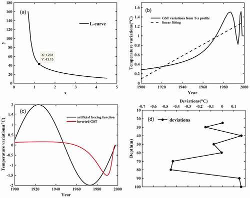
Figure 3. (a) L-curve for the Tikhonov regularization. $\alpha$ was about 0.016, corresponding to the corner of the curve. (b) The GST variations from the initial steady-state temperature in the last century reconstructed from Malan borehole temperatures. (c) The GST history (black line) and the reconstructed solution by the Tikhonov regularization (red line). (d) The deviations (dots) between the measurements and the calculated T–z profile

Results

Our results showed that the reconstruction performed in a shallow borehole (102 m) at Malan Glacier covered about one century, indicating the overall warming from the 1900s to 1990s (Figure 3b). A clear warming trend since the 1950s was found at Malan Glacier. The results showed that the GST increased about 1.1°C over the last century. The warmest period occurred in the 1980s to 1990s and the highest temperature variation could be 1.5°C to 1.6°C. The temperature decreased in the early 1990s and then increased again. It should be pointed out that the temperature variation in Figure 3b is the deviation of GST from the initial steady-state temperature (−4.8°C). We used the T–z profile data from below 15 m depth for inversion, and it showed a cooling over the most recent two years. This most likely reflected a temperature decrease between the 25- and 20-m depths in the measured T–z profile (Figure 1b).

Discussion

Resolution

Note that the reconstruction from glacier borehole temperatures only provides a long-term average temperature for a period. This is because the time resolution and the accuracy of the temperature variation decrease backward in time (Dahl-Jensen and Johnsen 1986). The time resolution depends on the depth of the drilled borehole and the specific GST variations. To examine the resolution of our inversion method, we used the 100-year-long GST curve of sinusoidal function as the input conditions to generate an artificial T–z profile and evaluated the corresponding GST history. We then compared the results with the artificial forcing function (Figure 3c). Through the 100-m-deep borehole, the temperature variations were not recovered before 1950s, and this technique was essentially multidecadal and could not provide information about annual temperature changes. The reconstruction showed more details in the last fifty years and was not able to compare the warming of the last few decades to the long-term context. The extrema of temperature were lower bounds of the actual GST history. The resolution of inversion appeared limited and was not improved by increasing or decreasing the temperature amplitude of sinusoidal function. In practice, any GST history derived from borehole temperatures will be a temporally “smeared” rendition of the actual GST history (Clow 1992).

Deviations

Deviations of the calculation data from the observed data are also shown in Figure 3d. Large deviations between the measurements and the calculated T–z profile were observed at depths of 70 and 80 m (Figure 3d), because large deviations were calculated between the measurements and the steady state at depths of 70 and 80 m (Figure 1b). Generally, as the depth increases, the perturbation in the borehole temperature becomes smaller, because the deeper it is, the more it is diffused out. Temperature variation in the glacier borehole is gradually smoothed as the depth increases. Indeed, if we look at Figure 1b we observed nonmonotonic parts of the T–z dependency at depth about 40 and 80 m. This means that the heat flux changed the sign. On the other hand, there was no reason to change the sign of the temperature gradient. In general case, the internal phase transition (heat production) can affect the sign of the temperature gradient. However, the temperature was below the melting point and there was no phase transition. In Figure 1b the large deviations can be attributed to insufficient time for borehole or thermometer equilibration and air circulation in the borehole. We would suspect that the borehole temperatures were affected by the air movements, so that despite the high precision of thermistors (0.01°C), the accuracy of measurements was a little bit worse. Thus, we smoothed the T–z profile (Figure 4a) to repeat reconstruction. The corresponding result is shown in Figure 4b.

Figure 4. (a) T–z profiles from measurements (black) and after smoothing (red). (b) The reconstructed GST histories from measurements (black line) and after smoothing the T–z profile (red line). The blue dashed line plots the linear fitting for the GST changes after smoothing the T–z profile

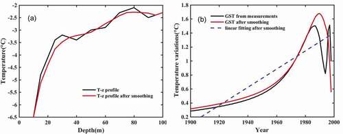
There were differences in the reconstruction between measurements and smoothing in Figure 4b. Although the T–z profile was smoother and more reasonable after smoothing, the temperature at 15 m was lower (−5.1°C), which led to larger deviations from the steady state. Thus, the GST history after smoothing the T–z profile was smoother and the maximum temperature rise was about 1.7°C. Such a warming trend contributed not only to the smoothing but also to the change of the steady state. The linear fitting after smoothing showed that the GST increased about 1.2°C over the last century, which was quite consistent with the results from measurements.

Comparison with other records

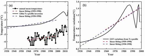
The ${\delta }^{18}O$ record in the Malan ice core, representing air temperature in the summer half year in the region, implied that it was warming by about 1.2°C over the last century (Wang et al. 2003). The comparison showed that the warming trend in the twentieth century reconstructed from borehole temperatures (1.1°C) was in agreement with that by ${\delta }^{18}O$ records (1.2°C) in the ice core. The results were also compared with nearby instrumental records by Wudaoliang meteorological station during periods of overlap. As shown in Figure 5, it was found that the warming trend from 1959 to 1998 by our GST reconstruction (about 0.16°C/10 years) was nearly consistent with that based on instrumental records (0.15°C/10a). This means that our reconstruction result for the twentieth century is highly reliable.

Figure 5. (a) Upper: the reconstruction based on the 120-m permafrost borehole drilled in 2012 (borehole temperatures measured in 2013) at Wudaoliang, along with the linear fitting from 1930 to 1998 (blue dashed line). (a) Lower: annual mean air temperature (dots) from 1959 to 2012 collected by Wudaoliang meteorological station and the linear fitting from 1959 to 1998 (red dashed line). (b) The reconstructed GST variations (solid line) and the linear fitting from 1959 to 1998 (red dashed line), along with the linear fitting from 1930 to 1998 (blue dashed line)

Comparison with other reconstructions

In recent decades, the history of climatic change has been reconstructed from glacier borehole temperatures on different timescales worldwide since the Last Glacial Maximum. Reconstructions spanning the past millennium or longer have concentrated on polar ice sheets because of the deep-drilled boreholes (1 km and deeper) with high measuring accuracy there (Dahl-Jensen and Johnsen 1986; Macayeal, Firestone, and Waddington 1991; Dahl-Jensen et al. 1998; Dahl-Jensen, Morgan, and Elcheikh 1999). Our reconstruction performed in the 102-m-deep borehole at Malan Glacier with measurement precision of 0.01°C covered only one century. Changes in GST for the past few hundred years or shorter also have been inferred from 90- to 500-m-deep boreholes at high latitudes and a high-elevation tropical site (Nagornov, Konovalov, and Tchijov 2006; Barrett et al. 2009; Gilbert et al. 2010; Zagorodnov et al. 2012). They all showed different levels of warming (about 1°C–5°C) over the twentieth century and most exceeded the average warming rate at Malan Glacier.

By comparing the temperature reconstructions from different boreholes nearby, researchers can better understand the climate changes on a regional scale. Our reconstruction was also compared with that from the 120-m permafrost borehole (35.22°N, 93.09°E, 4,668 m.a.s.l.) drilled in 2012 (borehole temperatures measured in 2013) at Wudaoliang meteorological station during periods of overlap (Figure 5; Liu 2015). The reconstruction from the permafrost borehole temperatures revealed warming of 1.1°C from 1930 to 1998, and our reconstructed GST at Malan Glacier increased 1.13°C during the same time. The comparison showed that the warming trend from 1930 to 1998 based on our reconstruction (0.161°C/10a) was in agreement with that from the permafrost borehole temperatures (0.157°C/10a). Furthermore, the temperature reconstructions from these two boreholes could confirm each other to a certain extent.

At present, models of coupled heat flow equations are common and few improvements in the accuracy to real physical processes remain to be developed (Macayeal, Firestone, and Waddington 1991; J. W. Yang et al. 2018). Most are based on the one-dimensional heat equation and employ the least squares inversion theory. All methods for inversion provide similar results, and compared with others, the Tikhonov regularization method is more stable to noise in the T–z profiles and requires fewer iterations to obtain the optimal solution for the model (Nagornov et al. 2017). When the drilling site is near the ice divide, the horizontal velocity of glacier layers in the model is negligible. It should be noted that the use of the one-dimensional model is not certainly worse than the two-dimensional or three-dimensional model. The one-dimensional techniques neglect the influences of numerous effects such as horizontal velocity, topography, and internal heat production. The application of the one-dimensional approach means that we use less parameters to describe the unknowns. And the development of the two-dimensional techniques will not necessarily improve the recovered GST variations. Though Dye-3 was far from the ice divide, a one-dimensional approach was also used by Macayeal, Firestone, and Waddington (Macayeal, Firestone, and Waddington 1991). The two-dimensional method may significantly increase the number of degrees of freedom of the inverse problem, though we may only get a finite amount of the measured information. With more complete knowledge of the past climatic changes, the reconstructed GST histories from borehole data will be more reliable (Louise and Vladimir 2007).

Conclusions

Most meteorological stations in the TP were established after the 1950s and are located in the eastern and southern TP. However, there are few stations over most of the northern and western TP, where there is a major area of high-elevation cryosphere and a lack of data on climate change. Therefore, reconstruction of the past climate change in the northern TP is very important for understanding the processes in the cryosphere there (especially permafrost, glaciers, and snow cover). Our nearly one-century temperature reconstruction by the Malan Glacier borehole temperatures provided a new result of climate change in the northern TP and indicated that about 1.1°C warming occurred in the twentieth century.

Borehole paleothermometry plays an important role in climate reconstruction. It is to a large extent credible and represents a supplement to instrumental records or proxy indicators. A comparison of temperature reconstructions spanning the past centuries and millennium indicates that at present few improvements in the accuracy or fidelity of the heat flow model remain to be developed. In order to obtain a more precise duration of the GST trends, future efforts should attempt to improve the measurement accuracy and extend measurements as deep as possible (Muto et al. 2011). Equally important, including additional information can improve the resolution and greatly enlarge the extent of the GST history that can be recovered (Louise and Vladimir 2007).

Acknowledgments

We thank all of the field team members from the Shaanxi Key Laboratory of Earth Surface System and Environmental Carrying Capacity and the CAS Center for Excellence in Tibetan Plateau Earth Sciences. Data sets for this research are included in Wang et al. (2006).

Disclosure statement

No potential conflict of interest was reported by the author(s).

Additional information

Funding

This research was supported by the Strategic Priority Research Program of the Chinese Academy of Sciences (Grant Nos. XDA20060201, XDA19070302) and the Second Tibetan Plateau Scientific Expedition and Research Program (Grant No. 2019QZKK020102).

References

- Barrett, B. E., K. W. Nicholls, T. Murray, A. M. Smith, and D. G. Vaughan. 2009. Rapid recent warming on Rutford Ice Stream, West Antarctica, from borehole thermometry. Geophysical Research Letters 36:L02708. doi:https://doi.org/10.1029/2008GL036369.
- Beltrami, H., and J. C. Mareschal. 1995. Resolution of ground temperature histories inverted from borehole temperature data. Global and Planetary Change 11:57–70. doi:https://doi.org/10.1016/0921-8181(95)00002-9.
- Bräuning, A., and B. Mantwill. 2004. Summer temperature and summer monsoon history on the Tibetan plateau during the last 400 years recorded by tree rings. Geophysical Research Letters 31:L24205. doi:https://doi.org/10.1029/2004gl020793.
- Broecker, W. S. 2001. PALEOCLIMATE: Was the medieval warm period global? Science 291 (5508):1497–99. doi:https://doi.org/10.1126/science.291.5508.1497.
- Calvetti, D., S. Morigi, L. Reichel, and F. Sgallari. 2000. Tikhonov regularization and the L-curve for large discrete ill-posed problems. Journal of Computational and Applied Mathematics 123 (1–2):423–46. doi:https://doi.org/10.1016/s0377-0427(00)00414-3.
- Chen, D. L., B. Q. Xu, T. D. Yao, Z. T. Guo, P. Cui, F. H. Chen, R. Zhang, X. Zhang, Y. Zhang, J. Fan, et al. 2015. Assessment of past, present and future environmental changes on the Tibetan Plateau. Chinese Science Bulletin 60 (32):3025–35. (in Chinese). doi:https://doi.org/10.1360/N972014-01370.
- Clow, G. D. 1992. The extent of temporal smearing in surface-temperature histories derived from borehole temperature measurement. Palaeogeography, Palaeoclimatology, Palaeoecology, 98:81–86. doi:https://doi.org/10.1016/0031-0182(92)90189-C.
- CMDSC. 2021. Meteorological data from the China Meteorological Data Service Center. Accessed March 5, 2021. http://data.cma.cn
- Dahl-Jensen, D., K. Mosegaard, N. Gundestrup, G. D. Clow, S. J. Johnsen, A. W. Hansen, and N. Balling. 1998. Past temperatures directly from the Greenland Ice Sheet. Science 282 (5387):268–71. doi:https://doi.org/10.1126/science.282.5387.268.
- Dahl-Jensen, D., and S. J. Johnsen. 1986. Palaeotemperatures still exist in the Greenland ice sheet. Nature 320:250–52. doi:https://doi.org/10.1038/320250a0.
- Dahl-Jensen, D., V. I. Morgan, and A. Elcheikh. 1999. Monte Carlo inverse modelling of the Law Dome (Antarctica) temperature profile. Annals of Glaciology 29:145–50. doi:https://doi.org/10.3189/172756499781821102.
- Gilbert, A., P. Wagnon, C. Vincent, P. Ginot, and M. Funk. 2010. Atmospheric warming at a high-elevation tropical site revealed by englacial temperatures at Illimani, Bolivia (6340m above sea level, 16°S, 67°W). Journal of Geophysical Research 115:D10109. doi:https://doi.org/10.1029/2009JD012961.
- Hotchkiss, W. O., and L. R. Ingersoll. 1934. Post-glacial time calculations from recent geothermal measurements in the Calumet copper mines. The Journal of Geology 42 (2):113–22. doi:https://doi.org/10.2307/30079563.
- Lachenbruch, A. H., and B. V. Marshall. 1986. Changing climate geothermal evidence from permafrost in the Alaskan Arctic. Science 234 (4777):689–96. doi:https://doi.org/10.1126/science.234.4777.689.
- Lane, E. C. 1923. Geotherms of the Lake Superior copper country. Bulletin of the Geological Society of America 34 (4):703–20. doi:https://doi.org/10.1130/gsab-34-703.
- Liu, J. 2015. Reconstruction of the past ground surface temperature changes using borehole paleothermometry. PhD dissertation, Lanzhou (in China). Lanzhou University.
- Louise, B., and C. Vladimir. 2007. Borehole climatology: A new method on how to reconstruct climate. 1st ed. Amsterdam: Elsevier Science. Accessed May 15, 2021. https://www.sciencedirect.com/book/9780080453200/borehole-climatology
- Macayeal, D. R., G. Firestone, and E. Waddington. 1991. Paleothermometry by control methods. Journal of Glaciology 37 (127):326–38. doi:https://doi.org/10.1017/S0022143000005761.
- Muto, A., T. A. Scambos, K. Steffen, A. G. Slater, and G. D. Clow. 2011. Recent surface temperature trends in the interior of East Antarctica from borehole firn temperature measurements and geophysical inverse methods. Geophysical Research Letters 38:L15502. doi:https://doi.org/10.1029/2011GL048086.
- Nagornov, O. V., S. A. Tyuflin, V. G. Nikitaev, and A. N. Pronichev. 2017. Comparative analysis of the past glacier surface temperatures based on various probe-functions. Journal of Physics: Conference Series 788:012055. doi:https://doi.org/10.1088/1742-6596/788/1/012055.
- Nagornov, O. V., Y. V. Konovalov, and V. Tchijov. 2006. Temperature reconstruction for Arctic glaciers. Palaeogeography, Palaeoclimatology, Palaeoecology, 236:125–34. doi:https://doi.org/10.1016/j.palaeo.2005.11.035.
- Nagornov, O. V., Y. V. Konovalov, V. S. Zagorodnov, and L. G. Thompson. 2001. Reconstruction of the surface temperature of Arctic glaciers from the data of temperature measurements in wells. Journal of Engineering Physics and Thermophysics 74 (2):253–65. doi:https://doi.org/10.1023/A:1016661616282.
- Nicholls, K. W., and J. G. Paren. 1993. Extending the Antarctic meteorological record using ice-sheet temperature profiles. Journal of Climate 6 (1):141–50. doi:https://doi.org/10.1175/1520-0442(1993)006<0141:etamru>2.0.co;2.
- Pu, J. C., T. D. Yao, and N. L. Wang. 2001. Recently variation of Malan Glacier in Hoh Xil region, center of Tibetan Plateau. Journal of Glaciology and Geocryology 23 (2):189–92. (in Chinese). Accessed May 15, 2021. http://en.cnki.com.cn/Article_en/CJFDTOTAL-BCDT200102013.htm
- Rodriguez, G., and D. Theis. 2005. An algorithm for estimating the optimal regularization parameter by the L-curve. Rendiconti di Matematica, Serie VII, 25: 69-84. Accessed May 15, 2021. https://www1.mat.uniroma1.it/ricerca/rendiconti/ARCHIVIO/2005(1)/69-84.pdf.
- USGS. 2021. Landsat TM data and digital elevation model data from United States Geological Survey. Accessed July 12, 2021. https://earthexplorer.usgs.gov/
- van de Wal, R. S. W., R. Mulvaney, E. Isaksson, J. C. Morre, J. F. Pinglot, V. A. Pohjola, M. P. A. Thomassen. 2002. Reconstruction of the historical temperature trend from measurements in a medium-length borehole on the Lomonosovfonna plateau, Svalbard. Annals of Glaciology 35:371–78. doi:https://doi.org/10.3189/172756402781816979.
- Wang, N. L., T. D. Yao, J. C. Pu, Y. L. Zhang, and W. Z. Sun. 2006. Climate change during the last 1000 years revealed by δ18O in the Malan ice core from the North Tibetan Plateau. Science in China, Series D 36 (8):723–32. (in Chinese). doi:https://doi.org/10.3969/j.1674-7240.2006.08.005.
- Wang, N. L., T. D. Yao, J. C. Pu, Y. L. Zhang, W. Z. Sun, and Y. Q. Wang. 2003. Variations in air temperature during the last 100 years revealed by δ18O in the Malan ice core from the Tibetan Plateau. Chinese Science Bulletin 48 (11):1219–23. (in Chinese). doi:https://doi.org/10.3321/j.0023-074X.2003.11.021.
- Xie, Z. C., J. K. Han, Q. H. Feng, and X. J. Wang. 2000. Primary study on the glaciers of Mountain Malan, Hoh Xil region, Qinghai-Xizang Plateau. Journal of Natural Science of Hunan Normal University 23 (1):83–66. (in Chinese). Accessed May 15, 2021. http://d.wanfangdata.com.cn/periodical/hnsfdx-zr200001019
- Yang, B., A. Bräuning, J. J. Liu, M. E. Davis, and Y. J. Shao. 2009. Temperature changes on the Tibetan Plateau during the past 600 years inferred from ice cores and tree rings. Global and Planetary Change 69 (1–2):71–78. doi:https://doi.org/10.1016/j.gloplacha.2009.07.008.
- Yang, J. W., Y. Han, A. J. Orsi, S. J. Kim, H. Han, Y. Ryu, Y. Jang, J. Moon, T. Choi, S. D. Hur, et al. 2018. Surface temperature in twentieth century at the Styx Glacier, northern Victoria Land, Antarctica, from borehole thermometry. Geophysical Research Letters 45 (18):9834–42. doi:https://doi.org/10.1029/2018GL078770.
- Yao, T. D., Y. K. Xue, D. L. Chen, F. H. Chen, L. Thompson, P. Cui, T. Koike, W. K.-M. Lau, D. Lettenmaier, and V. Mosbrugger. 2019. Recent Third Pole’s rapid warming accompanies cryospheric melt and water cycle intensification and interactions between monsoon and environment: Multi-disciplinary approach with observation, modeling and analysis. Bulletin of the American Meteorological Society 100 (3):423–44. doi:https://doi.org/10.1175/BAMS-D-17-0057.1.
- Zagorodnov, V., O. Nagornov, and L. G. Thompson. 2006. Influence of air temperature on a glacier’s active-layer temperature. Annals of Glaciology 43:285–91. doi:https://doi.org/10.3189/172756406781812203.
- Zagorodnov, V., O. Nagornov, T. A. Scambos, A. Muto, E. Mosley-Thompson, E. C. Pettit, and S. Tyuflin. 2012. Borehole temperatures reveal details of 20th century warming at Bruce Plateau, AntArctic Peninsula. The Cryosphere 6 (3):675–86. doi:https://doi.org/10.5194/tc-6-675-2012.