Variation in δ¹³C and δ¹⁵N within and among plant species in the alpine tundra

ABSTRACT

Ratios of carbon (C) and nitrogen (N) stable isotopes in plants are important indicators of intrinsic water use efficiency and N acquisition strategies. Here, we examined patterns of inter- and intraspecific variations and phylogenetic signal in foliar δ¹³C and δ¹⁵N for 59 alpine tundra plant species, stratifying our sampling across five habitat types. Overall, we found that variation in both δ¹³C and δ¹⁵N mirrored well-known patterns of water and nitrogen limitation among habitat types and that there was significant intraspecific trait variation in both δ¹³C and δ¹⁵N for some species. Lastly, we only found a strong signal of phylogenetic conservatism in δ¹³C in two habitat types and no phylogenetic signal in δ¹⁵N. Our results suggest that although local environmental conditions do play a role in determining variation in δ¹³C and δ¹⁵N among habitat types, there is considerable variation within and among species that is only weakly explained by shared ancestry. Taken together, our results suggest that considering local environmental variation, intraspecific trait variation, and shared ancestry can help with interpreting isotope patterns in nature and with predicting which species may be able to respond to rapidly changing environmental conditions.

KEYWORDS:

• Alpine
• δ¹³C
• δ¹⁵N
• intraspecific trait variation
• phylogenetic signal

Introduction

As trait-based approaches in community ecology are becoming more prevalent (e.g., Kraft, Valencia, and Ackerly 2008; Hulshof and Swenson 2010; Adler et al. 2013; Carmona et al. 2016), there has been an increased interest in understanding whether species’ traits vary predictably along environmental gradients (Díaz et al. 2007; Cornwell and Ackerly 2009; Spasojevic et al. 2014) and what shapes patterns of functional trait variation within and among species (Albert et al. 2010; Violle et al. 2012; Hulshof et al. 2013). Though it is increasingly evident that variation in plant functional traits among some species (or lack thereof) is a result of both selection by the environment (i.e., Bloor and Grubb 2004; Gratani 2014) and phylogenetic history (i.e., Cavender-Bares, Keen, and Miles 2006; Swenson and Enquist 2007), there is no clear indication of when one is more important (Flores et al. 2014; J. Yang et al. 2014; Forrestel, Ackerly, and Emery 2015; Bhaskar et al. 2016). Importantly, though many studies have examined environmentally driven inter- and intraspecific trait variability and phylogenetic history in plant morphological traits (i.e., Cavender-Bares et al. 2009), far fewer studies have examined these same patterns in plant stable isotopes (i.e., Goud and Sparks 2018; Prieto et al. 2018; Roscher et al. 2018; Vitória et al. 2018; Májeková et al. 2021).

The isotopes of two key elements that are linked to physiological processes are ¹³C and ¹⁵N. Foliar carbon isotope (δ¹³C) values in plants are related to the balance of photosynthesis and foliar water loss and their coupled response to variation in the environment (Farquhar, Oleary, and Berry 1982; Farquhar, Ehleringer, and Hubick 1989; Cernusak et al. 2013). Specifically, δ¹³C is controlled by the ratio of intercellular (c_i) to ambient (c_a) CO₂ concentrations where plants become enriched in ¹³C by any process that increases the difference between c_i and c_a (Farquhar, Oleary, and Berry 1982). Importantly, there is a significant relationship between c_i/c_a and plant intrinsic water use efficiency (iWUE), where δ¹³C provides an estimate of the long-term iWUE of a plant (Ehleringer 1989; Farquhar, Ehleringer, and Hubick 1989). Some plants can rapidly respond to decreased water availability by increasing their iWUE and thus altering their δ¹³C, suggesting a key role for environmental variation in influencing differences in δ¹³C within and among species (Farquhar, Ehleringer, and Hubick 1989; Corcuera, Gil-Pelegrin, and Notivol 2010; Ramírez-Valiente et al. 2010). In contrast, some plants maintain their δ¹³C values when grown under different environmental conditions (Ehleringer 1989; Farquhar, Ehleringer, and Hubick 1989; Goud, Prehmus, and Sparks 2021), suggesting that variation in δ¹³C among species may be in part determined by the evolutionary history of a species (Korner, Farquhar, and Wong 1991; Anderson et al. 1996; Y. Yang, Siegwolf, and Körner 2015).

Foliar nitrogen isotope (δ¹⁵N) values in plants can shed light on short-term dynamics of the N cycle (Craine et al. 2015), though variation in δ¹⁵N is much more difficult to explain than variation in δ¹³C. Variation in observed foliar δ¹⁵N within and among species is dependent on a combination of available nitrogen from atmospheric deposition, soils, or bedrock (Kolb and Evans 2002) and symbioses (e.g., mycorrhizal fungi and N-fixing rhizobia; E. A. Hobbie, Macko, and Williams 2000; J. E. Hobbie and Hobbie 2006). As seen with δ¹³C, foliar δ¹⁵N may be under stronger evolutionary control where species maintain δ¹⁵N values across gradients in N availability (Miller and Bowman 2003; Y. Yang, Siegwolf, and Körner 2015) or, alternatively, δ¹⁵N may vary greatly between conspecific individuals in response to differences in soil N availability (Bustamante et al. 2004).

To date there have been relatively few tests for a phylogenetic signal in C and N isotopes for plants, with most studies assuming that variation in C and N isotopes is largely a result of environmental variation. In one of the handful of studies to examine the relative roles of environment control and phylogenetic history in δ¹³C and δ¹⁵N for plants, Goud and Sparks (2018) found that both δ¹³C and δ¹⁵N exhibited significant trait conservatism (closely related species were more similar than expected by chance) for a group of fifty-seven plant species in the Ericaceae. Moreover, by sampling over broad environmental gradient including swamps and riparian zones in the southeastern United States, California chaparral, and arctic tundra in northern Canada, they found that phylogenetic history played a stronger role in influencing intraspecific variation in isotope values than the environment, except in some specialized environments (Goud and Sparks 2018). Similarly, Prieto et al. (2018) found that leaf δ¹³C was highly conserved across sites with different climate and environmental conditions, Májeková et al. (2021) found a strong phylogenetic signal for δ¹³C in graminoids, and Roscher et al. (2018) found a strong phylogenetic signal in δ¹⁵N, supporting the idea that phylogenetic history may have played a stronger role in influencing isotope values than local environmental variation. Though these studies provide an excellent broad-scale assessment of the roles of environment and phylogenetic history, we still lack a clear picture of whether these patterns are consistent across a broader phylogeny (multiple families), whether the relative importance of phylogenetic history and environmental variation differs at smaller spatial scales, and whether these patterns hold true for alpine tundra plants.

Here, we examined patterns of foliar δ¹³C and δ¹⁵N for 59 species across twenty plant families in alpine tundra. Due to the redistribution of snow by wind in the alpine tundra, strong gradients of productivity, soil moisture, nutrient availability, and physical stress result in a mosaic of habitat types across alpine tundra landscapes (Bowman and Fisk 2001; M. D. Walker et al. 2001; Bowman, Bahnj, and Damm 2003; Seastedt et al. 2004; Litaor, Williams, and Seastedt 2008). These habitat types include fellfield, dominated by cushion plants (Silene acaulis [Caryophyllaceae], Minuartia obtusiloba [Caryophyllaceae], and Trifolium dasyphyllum [Fabaceae]) and lichens; dry meadow, dominated by Kobresia myosuroides (Cyperaceae); moist meadow, co-dominated by Deschampsia caespitosa (Poaceae) and Geum rossii (Rosaceae); wet meadow, dominated by Carex scopulorum (Cyperaceae), Pedicularis groenlandica (Orobranchaceae), and Caltha leptosepala (Ranunculaceae); and late melting snowbanks, dominated by Carex pyrenaica (Cyperaceae) and Sibbaldia procumbens (Rosaceae; May and Webber 1982; D. A. Walker et al. 1993; M. D. Walker et al. 2001). Transitions among habitat types can be sharp, with transitions among habitat types occurring over gradients of 10 m or less in length (Spasojevic and Suding 2012). To better understand patterns of inter- and intraspecific trait variation in alpine plants, we examined patterns of inter- and intraspecific variations in foliar δ¹³C and δ¹⁵N across these habitat types and explored patterns of phylogenetic conservatism within and among habitat types. If environmental variation is a key determinant of δ¹³C and δ¹⁵N, then we would expect habitats to differ in species mean isotope values in ways that reflect known patterns of water and nitrogen limitation and that the species found in multiple habitat types would exhibit intraspecific trait variation (ITV) in δ¹³C and δ¹⁵N as individuals alter their isotope values in response to this environmental variation through either plasticity or local adaptation. If phylogenetic history strongly influences patterns of δ¹³C and δ¹⁵N, we expect stronger phylogenetic conservatism in δ¹³C and δ¹⁵N within and among habitats.

Methods

Study location

This study was conducted in alpine tundra at the Niwot Ridge Long Term Ecological Research (LTER) site (40°03′N, 105°35′W, 3,528 m.a.s.l.). Located in the Front Range of the Colorado Rocky Mountains, Niwot Ridge has a short growing season (approximately three months) with a mean annual temperature of −2.3°C (6.5°C in the growing season) and an average annual precipitation of 884 mm, with the majority of the precipitation (94 percent) falling as snow (Litaor, Williams, and Seastedt 2008). Annual daily wind speeds average 8.1 m s⁻¹, with an average annual daily maximum wind speed of 19.8 m s⁻¹ (Losleben and Chowanski unpublished data). Due to these high wind speeds, an important environmental factor in alpine tundra is the redistribution of snow by wind (Bowman and Fisk 2001). Wind keeps fellfield and dry meadow habitats relatively snow-free all winter, and these low-productivity habitats are characterized by temperature stress, low water availability, and low nitrogen availability (Billings and Mooney 1968; M. D. Walker et al. 2001). Blown snow accumulates in snowbank habitats, which are buffered from wind scour and temperature stresses in the winter and tend to be energy limited due to the large snow accumulation. Snowmelt during the growing season enhances water and nitrogen availability in moist and wet meadow habitats found downhill of snowbank habitats. Soil moisture is significantly correlated with snowfall amounts and terrain factors that affect snow accumulation (Taylor and Seastedt 1994).

Trait collection

We collected leaves from fifty-nine species in twenty plant families and four functional groups (Supplementary Table 1) during the summers of 2017 and 2018. Samples were primarily collected next to eighty-eight permanent 1 m² plots (ranging in elevation from 3,506 to 3,568 m.a.s.l.) established in 1989 to track temporal changes in vegetation in the different habitat types found on Niwot Ridge (described above). Species for collection were chosen haphazardly within each community type and twenty of the fifty-nine species were found in multiple habitat types. For each species in each community type we collected one leaf from five to twenty separate individuals (all individuals were greater than 1 m apart to ensure that individuals were not clones connected belowground). Leaves were oven dried at 60°C for four days. Approximately 10 g of dry material was then shipped to the University of Wyoming Stable Isotope Facility (http://www.uwyo.edu/sif/) where samples were ground with a steel ball mil and analyzed for δ¹³C and δ¹⁵N on a Carlo Erba 1110 Elemental Analyzer coupled to a Thermo Delta V IRMS. Isotope ratios were calculated as,

Table 1. Across all alpine tundra habitat types and habitat specific values for Pagel’s λ

	Pagel’s λ
Habitat type	δ^13C	δ^15N
All habitat types	0.29	<0.01
Fellfield	0.43	0.75
Dry meadow	0.09	<0.01
Moist meadow	0.86	<0.01
Wet meadow	1.00	0.75
Snowbank	<0.01	0.14

Bold values indicate that Pagel’s λ was significantly greater than 0 (p < .05). Values equal to 1 suggest that the trait follows a Brownian process; values equal to 0 reflect the absence of any phylogenetic correlation; intermediate values indicate a weaker effect than expected from a Brownian motion model (Felsenstein 1985).

$\delta \left[{\hspace{0.17em}}^{13}\mathrm{C},\hspace{0.17em}{\hspace{0.17em}}^{15}\mathrm{N}\right]samples=\left(\frac{R_{sample}}{R_{standard}}-1\right)x1000$

where R_sample and R_standard are the ¹³C/¹²C or ¹⁵N/¹⁴N molar abundance ratios of samples, with 36-UWSIF-Glutamic 1 and 39-UWSIF-Glutamic 2 use as reference samples.

Phylogenetic tree

To evaluate the importance of evolutionary history, we created a synthesis-based phylogeny by subsetting our taxa from the time-calibrated molecular phylogeny of Zanne et al. (2014). We acknowledge that a purpose-built phylogeny would provide stronger inference, but many of the species at our site have yet to be sequenced. However, synthesis-based phylogenies have been shown to be robust for typical community ecology analyses, and trait phylogenetic signal estimated with synthesis-based phylogenies is highly correlated with estimates of Pagel’s λ from purpose-built phylogenies when traits are simulated under Brownian motion (Li et al. 2019; Qian and Jin 2021). Prior to calculations of phylogenetic signal, we first used the congeneric.merge function in the PEZ package, which binds missing species into the phylogeny by replacing all members of the clade it belongs to with a polytomy (Pearse et al. 2015). We then resolved polytomies using the multi2di function in the ape package (Paradis, Claude, and Strimmer 2004). Note that resolving polytomies in this way does not affect branch lengths and consequently maximum likelihood estimates of Pagel’s λ do not vary. We then calculated Pagel’s λ (Pagel 1999) for δ values of both elements using the multiPhylosignal function in the PICANTE package in R (Kembel et al. 2010). We used Pagel’s λ to quantify phylogenetic signal, because it has been shown to be robust to branch length uncertainty and many of the calibration issues that affect supertrees (Münkemüller et al. 2012; Molina-Venegas and Rodríguez 2017). Pagel’s λ is a branch scaling parameter that ranges from 0 to 1, where a λ values of 0 indicate no phylogenetic signal and a λ value of 1 indicates a phylogenetic signal found under a Brownian motion model of trait evolution (Pagel 1999). We then used the contMap function in the phytools package (Revell 2012) to plot isotope values along our trimmed phylogeny. All phylogenetic analyses were conducted in R (R Core Team 2019).

Statistical analysis

To test for differences in species mean isotopic values among habitat types we used a one-way analysis of variance and Tukey’s post hoc comparisons to compare each habitat type. To compare intraspecific variation in isotope values among habitats for the twenty species found in multiple habitats, we used a one-way analysis of variance and Tukey’s post hoc comparisons to compare values among each habitat type. Both analyses were conducted in JMP version 13 (SAS 2021).

To assess the degree to which closely related species were more similar to each other in isotope values than expected by chance, we tested whether Pagel’s λ was greater than 0 by comparing the log-likelihood of the fitted λ with that of λ = 0 using a log-likelihood ratio test using the “phylosig” function in the phytools R package (Revell 2012). Variables with a λ greater 0.5 (at p = .05) have a phylogenetic signal (i.e., closely related species are more similar to each other than expected by random chance; Münkemüller et al. 2012).

Results

Habitat variation

We found that species mean isotope signatures varied among habitats for both δ¹³C and δ¹⁵N (F_4,81 = 3.29, p = .01 and F_4,81 = 3.31, p = .01 respectively; Figure 1), with the least negative δ¹³C in dry meadow and the most negative in wet meadow and the highest values for δ¹⁵N in wet meadow and the lowest in fellfield. Tukey’s post hoc comparisons revealed that only dry meadow and wet meadow significantly differed from each other in δ¹³C (Figure 1), and only wet meadow and fellfield significantly differed in δ¹⁵N (Figure 1).

Figure 1. Variation in (a) δ¹³C and (b) δ¹⁵N among habitat types in alpine tundra. Each data point represents a species-level mean. The longer horizontal line represents the mean value for each habitat type and shorter horizontal lines represent the standard error of the mean. Letters represent significant differences among habitat types based on Tukey’s post hoc comparisons.

Intraspecific trait variation

We found that most species exhibited some degree of ITV in δ¹³C either within or among habitat types (Figure 2, Appendix). Thirteen of the twenty species that we sampled exhibited shifts in mean δ¹³C values across habitat types. Most of these species exhibited higher δ¹³C values in drier habitats (as expected), yet a few species showed idiosyncrasies. Geum rossii had its most negative values in fellfield habitat and highest in snowbank habitats. This species is known to preform leaves up to two years ahead of time, and it is unclear how preformation of leaves may influence δ¹³C. Festuca brachyphylla had much less negative δ¹³C values in dry meadow than in fellfield habitat types despite both being water limited.

Figure 2. Intraspecific variation in δ¹³C among species sampled in multiple habitat types in alpine tundra. Habitats with no data points indicate that species was not present in that habitat type. The longer horizontal line represents the mean value for each habitat type and shorter horizontal lines represent one standard deviation. Letters represent significant differences among habitat types based on Tukey’s post hoc comparisons. Species codes: (a) Artemisia scopulorum (Artsco); (b) Bistorta bistortoides (Bisbis); (c) Caltha leptosepala (Callep); (d) Carex rupestris (Carrup); (e) Carex scopulorum (Carsco); (f) Deschampsia caespitosa (Desces); (g) Erigeron simplex (Erisim); (h) Festuca brachyphylla (Fesbra); (i) Geum rossii (Geuros); (j) Kobresia myosuroides (Kobmyo); (k) Lloydia serotina (Lloser); (l) Luzula spicata (Luzspi); (m) Mertensia lanceolate (Merlan); (n) Minuartia obtusiloba (Minobt); (o) Oreoxis alpina (Orealp); (p) Ranunculus adoneus (Ranado); (q) Silene acaulis (Silaca); (r) Tetraneuris acaulis (Tetaca); (s) Trifolium dasyphyllum (Tridas); (t) Trifolium parryi (Tripar).

Similarly, most species exhibited some degree of ITV in δ¹⁵N either within or among habitat types (Figure 3, Appendix). Twelve of the twenty species that we sampled exhibited shifts in mean δ¹⁵N across habitat types. Most of these species exhibited higher δ¹⁵N values in habitats associated with higher N availability (wet meadow, moist meadow), but some species differed from this general pattern, which may reflect differences in resource uptake strategies. For example, Lloydia serotina had higher δ¹⁵N values in fellfield and dry meadow habitats than in moist meadow. Moreover, both N-fixing forbs (Trifolium parryi and T. dasyphyllum) had species mean δ¹⁵N values that were negative indicating uptake of nitrogen from the soil in addition to N fixation.

Figure 3. Intraspecific variation in δ¹⁵N among species sampled in multiple habitat types in alpine tundra. Habitats with no data points indicate that species was not present in that habitat type. The longer horizontal line represents the mean value for each habitat type and shorter horizontal lines represent one standard deviation. Letters represent significant differences among habitat types based on Tukey’s post hoc comparisons. Species codes: (a) Artemisia scopulorum (Artsco); (b) Bistorta bistortoides (Bisbis); (c) Caltha leptosepala (Callep); (d) Carex rupestris (Carrup); (e) Carex scopulorum (Carsco); (f) Deschampsia caespitosa (Desces); (g) Erigeron simplex (Erisim); (h) Festuca brachyphylla (Fesbra); (i) Geum rossii (Geuros); (j) Kobresia myosuroides (Kobmyo); (k) Lloydia serotina (Lloser); (l) Luzula spicata (Luzspi); (m) Mertensia lanceolate (Merlan); (n) Minuartia obtusiloba (Minobt); (o) Oreoxis alpina (Orealp); (p) Ranunculus adoneus (Ranado); (q) Silene acaulis (Silaca); (r) Tetraneuris acaulis (Tetaca); (s) Trifolium dasyphyllum (Tridas); (t) Trifolium parryi (Tripar).

Lastly, we found seven species exhibiting ITV in δ values of both elements, and three species exhibited no ITV in isotope composition of both elements. These three species included a sedge (Carex rupestris), a forb (Oreoxis alpine), and an N-fixing forb (Trifolium parryi) that are most abundant in different habitat types and have little in common. Lastly, we found no general patterns in ITV within or among functional groups with some grasses, some forbs, and some N fixers exhibiting significant ITV in both isotopes, some in only one isotope, and some exhibiting no ITV in either.

Phylogenetic signal

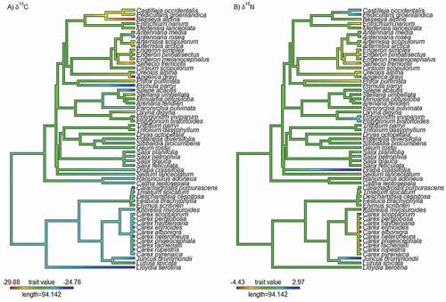
Across all alpine tundra habitat types, we found evidence for a weak phylogenetic signal in δ¹³C (Pagel’s λ = 0.29; Figure 4, Table 1) where phylogenetic signal was significantly greater than 0 (p < .01), but the phylogeny exerts a weaker effect on the trait evolutionary process than expected from a Brownian motion model. For δ¹⁵N we found no evidence of a phylogenetic signal (Pagel’s λ < 0.01; Figure 4, Table 1) and it did not significantly differ from 0 (p = 1). Within habitats we found evidence for stronger trait conservatism in δ¹³C only in moist meadow (Pagel’s λ = 0.86, p < .01; Table 1) and wet meadow (Pagel’s λ = 1.0, p < .01; Table 1) and no significant phylogenetic signal in δ¹⁵N in any habitat type (Table 1).

Figure 4. Phylogenetic patterns of variation in (a) δ¹³C and (b) δ¹⁵N among plant species in alpine tundra across all alpine tundra habitat types. We found a weak phylogenetic signal in δ¹³C (Pagel’s λ = 0.29) where phylogenetic signal was significantly greater than 0 (p = .004).

Discussion

Though many studies have generally assumed strong role of environmental variation in influencing patterns of plant δ¹³C and δ¹⁵N, we found a much more nuanced picture. When we examined isotope patterns across all tundra habitats, we found isotopic signatures that largely mirror the patterns expected given the known environmental heterogeneity in this system (i.e., greater moisture and nitrogen limitation in fellfield and dry meadow). However, some species exhibited ITV in isotope values that matched environmental gradients and some species did not. Moreover, we found evidence for phylogenetic conservatism in only a few habitat types but only for δ¹³C, suggesting that phylogenetic history has a modest influence on isotope values. Together, these results suggest that while species sorting is occurring generally at the habitat scale (i.e., more water use–efficient species are generally in more water-limited habitats), individual species may have evolved a variety of strategies for coping with the strong environmental gradients in alpine tundra. Importantly, these species-specific patterns may be indicative of a species’ potential to cope with changing environmental conditions (i.e., Botero et al. 2015) where some species are able to plastically respond to changing environmental conditions and some species are not (Lauteri et al. 2004; Nicotra et al. 2010).

Habitat variation

We found that when examining the overall patterns among species (ignoring ITV), isotope values generally varied among habitats in a manner mirroring well-established differences among habitats in water and nitrogen availability (e.g., Bowman and Fisk 2001; M. D. Walker et al. 2001; Bowman, Bahnj, and Damm 2003; Seastedt et al. 2004; Litaor, Williams, and Seastedt 2008). We found the highest average δ¹³C in dry meadow and the lowest in δ¹³C wet meadow, which, as their names indicate, differ significantly in soil moisture. Although we lack on-the-ground measurements of soil moisture, we can see predictable changes in δ¹³C in the tundra, with the driest habitats (dry meadow and fellfield) having the species with the highest iWUE, moist meadow having species with intermediate iWUE, and the wettest habitats (wet meadow and snowbank) having the species with the lowest iWUE. Similarly, we found the highest average δ¹⁵N in wet meadow and the lowest average δ¹⁵N in the fellfield. Patterns of nitrogen limitation in the alpine largely mirror pattern of water limitation, with the lower nitrogen availability in dry meadow and fellfield and higher nitrogen availability in moist meadow, wet meadow, and snowbank habitats (Bowman, Bahnj, and Damm 2003). Similarly, Y. Yang, Siegwolf, and Körner (2015) found variation in both δ¹³C and δ¹⁵N along an elevation gradient in the Swiss alpine, further suggesting that environmental variation influences foliar isotopes in alpine plant species. Though our results unsurprisingly suggest that environmental variation influences variation in foliar stable isotopes among habitat types, pattern of ITV within individual species and patterns of phylogenetic signal suggest that more nuance is needed when considering isotope patterns.

Intraspecific trait variation

In addition to predictable variation among habitats, we found significant ITV in either δ¹³C or δ¹⁵N for most (seventeen out of twenty) of the species that occurred across multiple habitat types. Twelve of these twenty species exhibited ITV in δ¹³C (Figure 2), suggesting that some species are able to modify their iWUE to cope with variation in water availability through either phenotypic plasticity or local adaptation (Cleland et al. 2007; Albert et al. 2011; Botero et al. 2015). Interestingly, eight species did not respond to the habitat-scale variation in water availability, suggesting that these species may be under stronger genetic control (Albert et al. 2011) or may have a less flexible bet hedging strategy for coping with different environmental variation (Botero et al. 2015). Similarly, twelve of twenty species exhibited ITV in δ¹⁵N (Figure 3; though not the same twelve species as δ¹³C), again suggesting that some species are able modify their phenotype to cope with variation in nitrogen availability and others are not. In total, sevven species exhibited significant ITV in both δ¹³C and δ¹⁵N among habitat types. Overall, these results suggest that some alpine plant species are highly variable and are able to adjust their phenotype to a wide range of variability in both water and nitrogen. These species are likely the least threatened by changing environmental conditions in the alpine (H. F. Diaz, Grosjean, and Graumlich 2003) and likely have the greatest capacity to adapt to changing environments (Botero et al. 2015) if this variation is associated with phenotypic plasticity. Of the seven species we found to have ITV in both isotopes, four (Artemisia scopulorum, Caltha leptosepala, Lloydia serotine, Luzula spicata) were found to be increasing in abundance over a twenty-one-year period in long-term monitoring plots (Spasojevic et al. 2013), two species remained stable (Bistorta bistortoides, Ranunculus adoneus), and only one was declining in abundance (Geum rossii). Interestingly, some of these species (Artemisia scopulorum, Luzula spicata, Ranunculus adoneus) show matching responses across habitats for both isotopes (highest and lowest values in similar habitats), and the other four species show no discernable pattern among isotopes. Future research examining ITV across a wider range of species or systems with less species turnover among habitats may help resolve the drivers of ITV in isotopes.

Interestingly, several of our species are able to adjust their phenotype to a wide range of conditions for one resource (i.e., nitrogen) but are unable to adjust their phenotype for another (i.e., water), suggesting that a species’ ability to track changing environmental condition will depend on which resource is changing the most rapidly. At our study site, atmospheric nitrogen deposition had reached critical levels (Bowman et al. 2006) and resulted in changes in some alpine plant communities (Simkin et al. 2016; Bowman et al. 2018). At the same time, Niwot Ridge is experiencing extended summers (prolonged midsummer drought; Niwot Ridge LTER unpublished data)which is reducing soil moisture during the growing season. Interestingly, we found that four of the five species that exhibit ITV in only δ¹³C are increasing in abundance over time in our long-term monitoring plots (Spasojevic et al. 2013), whereas only two of five species that exhibit ITV in only δ¹⁵N are increasing over time in those same plots. These patterns suggest that species that exhibit ITV in iWUE may be less at risk to environmental change than species that exhibit ITV in their nitrogen acquisition strategy. Importantly, these two global change drivers interact (water availability influences nitrogen availability; Bowman et al. 1993; Bowman, Bahnj, and Damm 2003), making predictions of species changes much more complex.

Three (out of twenty) species in our data set—the sedge Carex rupestris, the forb Oreoxis alpine, and the N-fixing forb Trifolium parryi—exhibited no ITV in either isotope, suggesting that isotopic variation may be less plastic for these three species. Similarly, Y. Yang, Siegwolf, and Körner (2015) found that isotope values for several congeners to our study species in the Swiss Alps were also insensitive to obvious environmental control, further suggesting that some species may have limited capacity to adjust their phenotypes in response to changing environmental conditions. Though these species likely have the least ability to cope with rapid environmental change through plastic changes (Botero et al. 2015), we do not see large changes in their abundance through time in our monitoring plots—only T. parryi is decreasing significantly through time and only in snowbank communities—suggesting that they may cope with environmental change with other strategies such as bet hedging (Botero et al. 2015) or simply being stress tolerant (Damschen et al. 2012).

Taken together, our results suggest that species have a broad range of mechanisms for coping with environmental variation, and patterns of ITV for C and N isotopes can help elucidate some of them. It is important to note that though previous studies have noted that phenotypic plasticity occurs in several congeners of our study species, we lack any data on population genetic structure of these species to know whether local adaptation or phenotypic plasticity is the mechanism underlying ITV in δ¹³C or δ¹⁵N. Future research linking population genetics and isotopes can help clarify the capacity for species to cope with changing environmental condition in the alpine tundra.

Phylogenetic signal

Unlike Goud and Sparks (2018), who found a strong phylogenetic signal in δ¹³C and δ¹⁵N, we found a weaker (though significant) phylogenetic signal than expected under a Brownian motion model of trait evolution when looking across all alpine tundra habitat types. We only found a strong phylogenetic signal when we focused in on particular habitat types and only for δ¹³C. This difference between our results and the results of Goud and Sparks (2018) may be related to the scale of our studies; Goud and Sparks (2018) focused on a single plant family (the Ericaceae), whereas we examined fifty-nine species across twenty families including both monocots and dicots. Though we lack the resolution to examine phylogenetic signal within families (we typically only have a few species within a given family), we do see that both the Salicaceae (willows) and Cyperaceae (sedges) all have species with similar values of δ¹³C. Interestingly, in the Cyperaceae we found both the highest and lowest species values for δ¹⁵N in this family. Nitrogen is a limiting resource in the tundra, and evidence suggests that some species coexist by partitioning different forms of nitrogen (Miller and Bowman 2003; Miller, Bowman, and Suding 2007; Ashton et al. 2008). Though this has not been explored experimentally within the genus Carex for these species, this pattern suggests that these sedges are potentially using different sources of nitrogen. Though some sedge species are spatially segregated (i.e., Carex rupestris and Carex scopulorum are largely found in different habitats), in our data set we sampled six species of sedge that co-occur in dry meadow and five species of sedge that co-occur in moist meadow, suggesting that nitrogen partitioning may be a way in which these closely related species co-occur (Silvertown 2004).

Though we only found a modest signal of phylogenetic conservatism in δ¹³C when looking across all of our alpine tundra habitat types, we did find a stronger phylogenetic signal in δ¹³C within moist and wet meadow tundra habitats, suggesting that δ¹³C values were significantly more similar among closely related species than expected by chance. We found no significant signal for the other habitat types. This pattern suggests that plant species in these wetter habitats are converging on similar functional strategies within a given family and that different strategies may have evolved among different families. Despite the long history of stable isotope studies, few studies have examined phylogenetic signal, and our results coupled with the results of Goud and Sparks (2018) suggest that more studies are needed across a larger portion of the plant phylogenetic tree to truly understand the degree of phylogenetic conservatism in plant stable isotopes. Importantly, we also acknowledge that our synthesis-based phylogeny limits our ability to delve deeper into the phylogenetic relationships we observe, and we encourage future researchers to sequence more alpine plant species.

Conclusions

Our results suggest that the significant inter- and intraspecific variations in C and N isotopes in alpine tundra plants mostly reflects known environmental gradients. However, though we found that significant variation among habitats mirroring predicted resource limitation, these patterns did not hold for all species and some species did not vary among habitat types. These patterns coupled with modest evidence for phylogenetic conservatism in δ¹³C suggest that considering local environmental variation, ITV, and shared ancestry can help with interpreting isotope patterns in nature and with predicting which species may be able to respond to rapidly changing environmental conditions.

Acknowledgments

We thank Courtney Collins for help with sample preparation, the University of Wyoming Stable Isotope Facility for isotope analyses, and Kenya Gates for help in the field.

Disclosure statement

No potential conflict of interest was reported by the authors.

Supplementary material

Supplemental material for this article can be accessed on the publisher’s website

Additional information

Funding

Financial and logistic support was provided by the National Science Foundation (DEB 1457827), the University of Colorado Mountain Research Station, and the Niwot Ridge LTER.

Appendix

Significance (F values, degrees of freedom, and p values) for all comparisons in Figure 2 for intraspecific variation in δ¹³C: (A) Artemisia scopulorum (F_4,47 = 5.26, p < .01); (B) Bistorta bistortoides (F_3,41 = 5.29, p < .01); (C) Caltha leptosepala (F_2,27 = 10.13, p < .01); (D) Carex rupestris (F_2,26 = 2.57, p = .09); (E) Carex scopulorum (F_2,32 = 7.10, p < .01); (F) Deschampsia caespitosa (F_3,43 = 2.37, p = .08); (G) Erigeron simplex (F_2,23 = 0.75, p = .48); (H) Festuca brachyphylla (F_1,26 = 14.71, p < .01); (I) Geum rossii (F_4,49 = 6.39, p < .01); (J) Kobresia myosuroides (F_1,13 = 3.66, p = .07); (K) Lloydia serotina (F_2,22 = 10.75, p < .01); (L) Luzula spicata (F_1,10 = 5.38, p = .04); (M) Mertensia lanceolate (F_2,23 = 1.94, p = .17); (N) Minuartia obtusiloba (F_3,36 = 10.19, p < .01); (O) Oreoxis alpina (F_1,18 = 1.35, p = .26); (P) Ranunculus adoneus (F_1,18 = 7.76, p = .01); (Q) Silene acaulis (F_1,18 = 12.39, p < .01); (R) Tetraneuris acaulis (F_1,18 = 0.26, p = .63); (S) Trifolium dasyphyllum (F_1,17 = 5.72, p = .03); (T) Trifolium parryi (F_2,29 = 1.14, p = .33);for all comparisons in Figure 3 for intraspecific variation in δ¹⁵N (A) Artemisia scopulorum (F_4,47 = 4.19, p < .01); (B) Bistorta bistortoides (F_3,41 = 4.01, p = .01); (C) Caltha leptosepala (F_2,27 = 1.86, p < .01); (D) Carex rupestris (F_2,26 = 1.48, p = .25); (E) Carex scopulorum (F_2,32 = 1.09, p = .35); (F) Deschampsia caespitosa (F_3,43 = 4.78, p < .01); (G) Erigeron simplex (F_2,23 = 7.19, p < .01); (H) Festuca brachyphylla (F_1,26 = 1.34, p = .26); (I) Geum rossii (F_4,49 = 7.59, p < .01); (J) Kobresia myosuroides (F_1,13 = 16.18, p < .01); (K) Lloydia serotina (F_2,22 = 10.28, p < .01); (L) Luzula spicata (F_1,10 = 14.15, p < .01); (M) Mertensia lanceolate (F_2,23 = 15.44, p < .01); (N) Minuartia obtusiloba (F_3,36 = 1.09, p = .36); (O) Oreoxis alpina (F_1,18 = 1.00, p = .33); (P) Ranunculus adoneus (F_1,18 = 28.88, p < .01); (Q) Silene acaulis (F_1,18 = 0.00, p = .97); (R) Tetraneuris acaulis (F_1,18 = 13.92, p < .01); (S) Trifolium dasyphyllum (F_1,17 = 1.42, p = .25); (T) Trifolium parryi (F_2,29 = 0.08, p = .92).

References

- Adler, P. B., A. Fajardo, A. R. Kleinhesselink, and N. J. B. Kraft. 2013. Trait-based tests of coexistence mechanisms. Ecology Letters 16:1294–306. doi:https://doi.org/10.1111/ele.12157.
- Albert, C. H., F. Grassein, F. M. Schurr, G. Vieilledent, and C. Violle. 2011. When and how should intraspecific variability be considered in trait-based plant ecology? Perspectives in Plant Ecology Evolution and Systematics 13:217–25. doi:https://doi.org/10.1016/j.ppees.2011.04.003.
- Albert, C. H., W. Thuiller, N. G. Yoccoz, A. Soudant, F. Boucher, P. Saccone, and S. Lavorel. 2010. Intraspecific functional variability: Extent, structure and sources of variation. Journal of Ecology 98:604–13. doi:https://doi.org/10.1111/j.1365-2745.2010.01651.x.
- Anderson, J. E., J. Williams, P. E. Kriedemann, M. P. Austin, and G. D. Farquhar. 1996. Correlations between carbon isotope discrimination and climate of native habitats for diverse eucalypt taxa growing in a common garden. Australian Journal of Plant Physiology 23:311–20.
- Ashton, I. W., A. E. Miller, W. D. Bowman, and K. N. Suding. 2008. Nitrogen preferences and plant-soil feedbacks as influenced by neighbors in the alpine tundra. Oecologia 156:625–36. doi:https://doi.org/10.1007/s00442-008-1006-1.
- Bhaskar, R., S. Porder, P. Balvanera, and E. J. Edwards. 2016. Ecological and evolutionary variation in community nitrogen use traits during tropical dry forest secondary succession. Ecology 97:1194–206. doi:https://doi.org/10.1890/15-1162.1.
- Billings, W. D., and H. A. Mooney. 1968. Ecology of arctic and alpine plants. Biological Reviews of the Cambridge Philosophical Society 43:481–529. doi:https://doi.org/10.1111/j.1469-185X.1968.tb00968.x.
- Bloor, J., and P. Grubb. 2004. Morphological plasticity of shade‐tolerant tropical rainforest tree seedlings exposed to light changes. Functional Ecology 18:337–48. doi:https://doi.org/10.1111/j.0269-8463.2004.00831.x.
- Botero, C. A., F. J. Weissing, J. Wright, and D. R. Rubenstein. 2015. Evolutionary tipping points in the capacity to adapt to environmental change. Proceedings of the National Academy of Sciences 112:184–89. doi:https://doi.org/10.1073/pnas.1408589111.
- Bowman, W. D., A. Ayyad, C. P. Bueno de Mesquita, N. Fierer, T. S. Potter, and S. Sternagel. 2018. Limited ecosystem recovery from simulated chronic nitrogen deposition. Ecological Applications 28:1762–72. doi:https://doi.org/10.1002/eap.1783.
- Bowman, W. D., J. R. Gartner, K. Holland, and M. Wiedermann. 2006. Nitrogen critical loads for alpine vegetation and terrestrial ecosystem response: Are we there yet? Ecological Applications 16:1183–93. doi:https://doi.org/10.1890/1051-0761(2006)016[1183:NCLFAV]2.0.CO;2.
- Bowman, W. D., L. Bahnj, and M. Damm. 2003. Alpine landscape variation in foliar nitrogen and phosphorus concentrations and the relation to soil nitrogen and phosphorus availability. Arctic, Antarctic, and Alpine Research 35:144–49. doi:https://doi.org/10.1657/1523-0430(2003)035[0144:ALVIFN]2.0.CO;2.
- Bowman, W. D., and M. C. Fisk. 2001. Primary production. In Structure and function of an alpine ecosystem, ed. W. D. Bowman and T. R. Seastedt, 177–97. New York, NY: Oxford University Press.
- Bowman, W. D., T. A. Theodose, J. C. Schardt, and R. T. Conant. 1993. Constraints of nutrient availability on primary production in two alpine tundra communities. Ecology 74:2085–97. doi:https://doi.org/10.2307/1940854.
- Bustamante, M. M. D. C., L. A. Martinelli, D. Silva, P. B. D. Camargo, C. Klink, T. F. Domingues, and R. Santos. 2004. 15N natural abundance in woody plants and soils of central Brazilian savannas (cerrado). Ecological Applications 14:200–13. doi:https://doi.org/10.1890/01-6013.
- Carmona, C. P., F. de Bello, N. W. H. Mason, and J. Leps. 2016. Traits without borders: Integrating functional diversity across scales. Trends in Ecology & Evolution 31:382–94. doi:https://doi.org/10.1016/j.tree.2016.02.003.
- Cavender-Bares, J., A. Keen, and B. Miles. 2006. Phylogenetic structure of Floridian plant communities depends on taxonomic and spatial scale. Ecology 87:S109–S122. doi:https://doi.org/10.1890/0012-9658(2006)87[109:PSOFPC]2.0.CO;2.
- Cavender-Bares, J., K. H. Kozak, P. V. A. Fine, and S. W. Kembel. 2009. The merging of community ecology and phylogenetic biology. Ecology Letters 12:693–715. doi:https://doi.org/10.1111/j.1461-0248.2009.01314.x.
- Cernusak, L. A., N. Ubierna, K. Winter, J. A. Holtum, J. D. Marshall, and G. D. Farquhar. 2013. Environmental and physiological determinants of carbon isotope discrimination in terrestrial plants. New Phytologist 200:950–65. doi:https://doi.org/10.1111/nph.12423.
- Cleland, E. E., I. Chuine, A. Menzel, H. A. Mooney, and M. D. Schwartz. 2007. Shifting plant phenology in response to global change. Trends in Ecology & Evolution 22:357–65. doi:https://doi.org/10.1016/j.tree.2007.04.003.
- Corcuera, L., E. Gil-Pelegrin, and E. Notivol. 2010. Phenotypic plasticity in Pinus pinaster δ 13 C: Environment modulates genetic variation. Annals of Forest Science 67:812–812. doi:https://doi.org/10.1051/forest/2010048.
- Cornwell, W. K., and D. D. Ackerly. 2009. Community assembly and shifts in plant trait distributions across an environmental gradient in coastal California. Ecological Monographs 79:109–26. doi:https://doi.org/10.1890/07-1134.1.
- Craine, J. M., E. Brookshire, M. D. Cramer, N. J. Hasselquist, K. Koba, E. Marin-Spiotta, and L. Wang. 2015. Ecological interpretations of nitrogen isotope ratios of terrestrial plants and soils. Plant and Soil 396:1–26. doi:https://doi.org/10.1007/s11104-015-2542-1.
- Damschen, E. I., S. Harrison, D. D. Ackerly, B. M. Fernandez-Going, and B. L. Anacker. 2012. Endemic plant communities on special soils: Early victims or hardy survivors of climate change? Journal of Ecology 100:1122–30. doi:https://doi.org/10.1111/j.1365-2745.2012.01986.x.
- Diaz, H. F., M. Grosjean, and L. Graumlich. 2003. Climate variability and change in high elevation regions: Past, present and future. Climatic Change 59:1–4. doi:https://doi.org/10.1023/A:1024416227887.
- Díaz, S., S. Lavorel, S. U. E. McIntyre, V. Falczuk, F. Casanoves, D. G. Milchunas, C. Skarpe, G. Rusch, M. Sternberg, I. Noy-Meir, et al. 2007. Plant trait responses to grazing? A global synthesis. Global Change Biology 13:313–41. doi:https://doi.org/10.1111/j.1365-2486.2006.01288.x.
- Ehleringer, J. R. 1989. Carbon isotope ratios and physiological processes in aridland plants. In Stable isotopes in ecological research, ed. P. W. Rundel, J. R. Ehleringer, and K. A. Nagy, 41–54. New York: Springer.
- Farquhar, G. D., J. R. Ehleringer, and K. T. Hubick. 1989. Carbon isotope discrimination and photosynthesis. Annual Review of Plant Physiology and Plant Molecular Biology 40:503–37. doi:https://doi.org/10.1146/annurev.pp.40.060189.002443.
- Farquhar, G. D., M. H. Oleary, and J. A. Berry. 1982. On the relationship between carbon isotope discrimination and the inter-cellular carbon-dioxide concentration in leaves. Australian Journal of Plant Physiology 9:121–37.
- Felsenstein, J. 1985. Phylogenies and the comparative method. American Naturalist 125:1–15. doi:https://doi.org/10.1086/284325.
- Flores, O., E. Garnier, I. J. Wright, P. B. Reich, S. Pierce, S. Diaz, R. J. Pakeman, G. M. Rusch, M. Bernard-Verdier, B. Testi, et al. 2014. An evolutionary perspective on leaf economics: Phylogenetics of leaf mass per area in vascular plants. Ecology and Evolution 4:2799–811. doi:https://doi.org/10.1002/ece3.1087.
- Forrestel, E. J., D. D. Ackerly, and N. C. Emery. 2015. The joint evolution of traits and habitat: Ontogenetic shifts in leaf morphology and wetland specialization in Lasthenia. New Phytologist 208:949–59. doi:https://doi.org/10.1111/nph.13478.
- Goud, E. M., and J. P. Sparks. 2018. Leaf stable isotopes suggest shared ancestry is an important driver of functional diversity. Oecologia 187:967–75. doi:https://doi.org/10.1007/s00442-018-4186-3.
- Goud, E. M., S. K. Prehmus, and J. P. Sparks. 2021. Is variation in inter-annual precipitation a mechanism for maintaining plant metabolic diversity? Oecologia 197:1039-1047. https://doi.org/https://doi.org/10.1007/s00442-021-05046-y.
- Gratani, L. 2014. Plant phenotypic plasticity in response to environmental factors. Advances in Botany 2014:1–17. doi:https://doi.org/10.1155/2014/208747.
- Hobbie, E. A., S. A. Macko, and M. Williams. 2000. Correlations between foliar δ15N and nitrogen concentrations may indicate plant-mycorrhizal interactions. Oecologia 122:273–83. doi:https://doi.org/10.1007/PL00008856.
- Hobbie, J. E., and E. A. Hobbie. 2006. 15N in symbiotic fungi and plants estimates nitrogen and carbon flux rates in arctic tundra. Ecology 87:816–22. doi:https://doi.org/10.1890/0012-9658(2006)87[816:NISFAP]2.0.CO;2.
- Hulshof, C. M., C. Violle, M. J. Spasojevic, B. J. McGill, E. I. Damschen, S. Harrison, and B. J. Enquist. 2013. Intraspecific and interspecific variation in specific leaf area reveal the importance of abiotic and biotic drivers of species diversity across elevation and latitude. Journal of Vegetation Science 921–31. doi:https://doi.org/10.1111/jvs.12041.
- Hulshof, C. M., and N. G. Swenson. 2010. Variation in leaf functional trait values within and across individuals and species: An example from a Costa Rican dry forest. Functional Ecology 24:217–23. doi:https://doi.org/10.1111/j.1365-2435.2009.01614.x.
- Kembel, S. W., P. D. Cowan, M. R. Helmus, W. K. Cornwell, H. Morlon, D. D. Ackerly, S. P. Blomberg, and C. O. Webb. 2010. Picante: R tools for integrating phylogenies and ecology. Bioinformatics 26:1463–64. doi:https://doi.org/10.1093/bioinformatics/btq166.
- Kolb, K. J., and R. D. Evans. 2002. Implications of leaf nitrogen recycling on the nitrogen isotope composition of deciduous plant tissues. New Phytologist 156:57–64. doi:https://doi.org/10.1046/j.1469-8137.2002.00490.x.
- Korner, C., G. D. Farquhar, and S. C. Wong. 1991. Carbon isotope discrimination by plants follows latitudinal and altitudinal trends. Oecologia 88:30–40. doi:https://doi.org/10.1007/BF00328400.
- Kraft, N. J. B., R. Valencia, and D. D. Ackerly. 2008. Functional traits and niche-based tree community assembly in an Amazonian forest. Science 322:580–82. doi:https://doi.org/10.1126/science.1160662.
- Lauteri, M., A. Pliura, M. Monteverdi, E. Brugnoli, F. Villani, and G. Eriksson. 2004. Genetic variation in carbon isotope discrimination in six European populations of Castanea sativa Mill. originating from contrasting localities. Journal of Evolutionary Biology 17:1286–96. doi:https://doi.org/10.1111/j.1420-9101.2004.00765.x.
- Li, D., L. Trotta, H. E. Marx, J. M. Allen, M. Sun, D. E. Soltis, P. S. Soltis, R. P. Guralnick, and B. Baiser. 2019. For common community phylogenetic analyses, go ahead and use synthesis phylogenies. Ecology 100:e02788. doi:https://doi.org/10.1002/ecy.2788.
- Litaor, M. I., M. Williams, and T. R. Seastedt. 2008. Topographic controls on snow distribution, soil moisture, and species diversity of herbaceous alpine vegetation, Niwot Ridge, Colorado. Journal of Geophysical Research-Biogeosciences 113. doi:https://doi.org/10.1029/2007JG000419.
- Májeková, M., T. Hájek, A. J. Albert, F. de Bello, J. Doležal, L. Götzenberger, Š. Janeček, J. Lepš, P. Liancourt, and O. Mudrák. 2021. Weak coordination between leaf drought tolerance and proxy traits in herbaceous plants. Functional Ecology 35:1299–311. doi:https://doi.org/10.1111/1365-2435.13792.
- May, D. E., and P. J. Webber. 1982. Spatial and temporal variation of the vegetation and its productivity, Niwot Ridge, Colorado. In Ecological studies in the Colorado Alpine: A festschrift for John W. Marr, ed. J. C. Halfpenny, 35–62. Boulder: Institue of Arctic and Alpine Research University of Colorado.
- Miller, A. E., and W. D. Bowman. 2003. Alpine plants show species-level differences in the uptake of organic and inorganic nitrogen. Plant and Soil 250:283–92. doi:https://doi.org/10.1023/A:1022867103109.
- Miller, A. E., W. D. Bowman, and K. N. Suding. 2007. Plant uptake of inorganic and organic nitrogen: Neighbor identity matters. Ecology 88:1832–40. doi:https://doi.org/10.1890/06-0946.1.
- Molina-Venegas, R., and M. Á. Rodríguez. 2017. Revisiting phylogenetic signal; strong or negligible impacts of polytomies and branch length information? BMC Evolutionary Biology 17:1–10.
- Münkemüller, T., S. Lavergne, B. Bzeznik, S. Dray, T. Jombart, K. Schiffers, and W. Thuiller. 2012. How to measure and test phylogenetic signal. Methods in Ecology and Evolution 3:743–56. doi:https://doi.org/10.1111/j.2041-210X.2012.00196.x.
- Nicotra, A. B., O. K. Atkin, S. P. Bonser, A. M. Davidson, E. Finnegan, U. Mathesius, P. Poot, M. D. Purugganan, C. L. Richards, and F. Valladares. 2010. Plant phenotypic plasticity in a changing climate. Trends in Plant Science 15:684–92. doi:https://doi.org/10.1016/j.tplants.2010.09.008.
- Pagel, M. 1999. Inferring the historical patterns of biological evolution. Nature 401:877. doi:https://doi.org/10.1038/44766.
- Paradis, E., J. Claude, and K. Strimmer. 2004. APE: Analyses of phylogenetics and evolution in R language. Bioinformatics 20:289–90. doi:https://doi.org/10.1093/bioinformatics/btg412.
- Pearse, W. D., M. W. Cadotte, J. Cavender-Bares, A. R. Ives, C. M. Tucker, S. C. Walker, and M. R. Helmus. 2015. Pez: Phylogenetics for the environmental sciences. Bioinformatics 31:2888–90. doi:https://doi.org/10.1093/bioinformatics/btv277.
- Prieto, I., J. I. Querejeta, J. Segrestin, F. Volaire, and C. Roumet. 2018. Leaf carbon and oxygen isotopes are coordinated with the leaf economics spectrum in Mediterranean rangeland species. Functional Ecology 32:612–25. doi:https://doi.org/10.1111/1365-2435.13025.
- Qian, H., and Y. Jin. 2021. Are phylogenies resolved at the genus level appropriate for studies on phylogenetic structure of species assemblages? Plant Diversity 43:255–63. doi:https://doi.org/10.1016/j.pld.2020.11.005.
- R Core Team. 2019. R: A language and environment for statistical computing. Vienna, Austria: R Foundation for Statistical Computing.
- Ramírez-Valiente, J. A., D. Sánchez-Gómez, I. Aranda, and F. Valladares. 2010. Phenotypic plasticity and local adaptation in leaf ecophysiological traits of 13 contrasting cork oak populations under different water availabilities. Tree Physiology 30:618–27. doi:https://doi.org/10.1093/treephys/tpq013.
- Revell, L. J. 2012. phytools: An R package for phylogenetic comparative biology (and other things). Methods in Ecology and Evolution 3:217–23. doi:https://doi.org/10.1111/j.2041-210X.2011.00169.x.
- Roscher, C., J. Schumacher, A. Lipowsky, M. Gubsch, A. Weigelt, B. Schmid, N. Buchmann, and E. D. Schulze. 2018. Functional groups differ in trait means, but not in trait plasticity to species richness in local grassland communities. Ecology 99:2295–307. doi:https://doi.org/10.1002/ecy.2447.
- SAS. 2021. JMP 13. Cary, NC: SAS Institute Inc.
- Seastedt, T. R., W. D. Bowman, T. N. Caine, D. McKnight, A. Townsend, and M. W. Williams. 2004. The landscape continuum: A model for high-elevation ecosystems. Bioscience 54:111–21. doi:https://doi.org/10.1641/0006-3568(2004)054[0111:TLCAMF]2.0.CO;2.
- Silvertown, J. 2004. Plant coexistence and the niche. Trends in Ecology & Evolution 19:605–11. doi:https://doi.org/10.1016/j.tree.2004.09.003.
- Simkin, S. M., E. B. Allen, W. D. Bowman, C. M. Clark, J. Belnap, M. L. Brooks, B. S. Cade, S. L. Collins, L. H. Geiser, and F. S. Gilliam. 2016. Conditional vulnerability of plant diversity to atmospheric nitrogen deposition across the United States. Proceedings of the National Academy of Sciences 113:4086–91. doi:https://doi.org/10.1073/pnas.1515241113.
- Spasojevic, M. J., E. A. Yablon, B. Oberle, and J. A. Myers. 2014. Ontogenetic trait variation influences tree community assembly across environmental gradients. Ecosphere 5:art129. doi:https://doi.org/10.1890/ES14-000159.1.
- Spasojevic, M. J., and K. N. Suding. 2012. Inferring community assembly mechanisms from functional diversity patterns: The importance of multiple assembly processes. Journal of Ecology 100:652–61. doi:https://doi.org/10.1111/j.1365-2745.2011.01945.x.
- Spasojevic, M. J., W. D. Bowman, H. C. Humphries, T. R. Seastedt, and K. N. Suding. 2013. Changes in alpine vegetation over 21 years: Are patterns across a heterogeneous landscape consistent with predictions? Ecosphere 4:art117. doi:https://doi.org/10.1890/ES13-00133.1.
- Swenson, N. G., and B. J. Enquist. 2007. Ecological and evolutionary determinants of a key plant functional trait: Wood density and its community‐wide variation across latitude and elevation. American Journal of Botany 94:451–59. doi:https://doi.org/10.3732/ajb.94.3.451.
- Taylor, R. V., and T. R. Seastedt. 1994. Short-term and long-term patterns of soil-moisture in alpine tundra. Arctic and Alpine Research 26:14–20. doi:https://doi.org/10.2307/1551871.
- Violle, C., B. J. Enquist, B. J. McGill, L. Jiang, C. H. Albert, C. Hulshof, V. Jung, and J. Messier. 2012. The return of the variance: Intraspecific variability in community ecology. Trends in Ecology & Evolution 27:244–52. doi:https://doi.org/10.1016/j.tree.2011.11.014.
- Vitória, A. P., E. Ávila-Lovera, T. de Oliveira Vieira, A. P. L. do Couto-Santos, T. J. Pereira, L. S. Funch, L. Freitas, L. D. A. P. De Miranda, P. J. P. Rodrigues, and C. E. Rezende. 2018. Isotopic composition of leaf carbon (δ13C) and nitrogen (δ15N) of deciduous and evergreen understorey trees in two tropical Brazilian Atlantic forests. Journal of Tropical Ecology 34:145–56. doi:https://doi.org/10.1017/S0266467418000093.
- Walker, D. A., J. C. Halfpenny, M. D. Walker, and C. A. Wessman. 1993. Long-term studies of snow-vegetation interactions. Bioscience 43:287–301. doi:https://doi.org/10.2307/1312061.
- Walker, M. D., D. A. Walker, T. A. Theodose, and P. J. Webber. 2001. The vegetation: Hierarchical species-environment relationships. In Structure and function of an alpine ecosystem, ed. W. D. Bowman and T. R. Seastedt, 99–127. Oxford: Oxford University Press.
- Yang, J., G. C. Zhang, X. Q. Ci, N. G. Swenson, M. Cao, L. Q. Sha, J. Li, C. C. Baskin, J. W. F. Slik, and L. X. Lin. 2014. Functional and phylogenetic assembly in a Chinese tropical tree community across size classes, spatial scales and habitats. Functional Ecology 28:520–29. doi:https://doi.org/10.1111/1365-2435.12176.
- Yang, Y., R. T. Siegwolf, and C. Körner. 2015. Species specific and environment induced variation of δ13C and δ15N in alpine plants. Frontiers in Plant Science 6:423. doi:https://doi.org/10.3389/fpls.2015.00423.
- Zanne, A. E., D. C. Tank, W. K. Cornwell, J. M. Eastman, S. A. Smith, R. G. FitzJohn, D. J. McGlinn, B. C. O’Meara, A. T. Moles, and P. B. Reich. 2014. Three keys to the radiation of angiosperms into freezing environments. Nature 506:89. doi:https://doi.org/10.1038/nature12872.