Soil organic carbon stocks in mountain periglacial areas of northern Patagonia (Argentina)

ABSTRACT

This study presents a detailed soil organic carbon (SOC) inventory for two areas in the mountain periglacial zone of northern Patagonia (altitude range c. 1,400–2,100 m). We describe plant cover and soil profiles at twenty-seven sites representing the main land cover classes and landform types at and above the treeline. The mean SOC 0–100 cm storage is 2.31 kg C m⁻² for the combined study areas, which includes 69 percent of bare ground surfaces with negligible SOC stocks. If we consider the vegetated alpine belt only, mean SOC 0–100 cm storage increases to 6.96 kg C m⁻². Solifluction has resulted in areas with dense plant cover and deep soil profiles with mean SOC 0–100 cm of 17.1 to 18.3 kg C m⁻² and a maximum total stock of 51.5 kg C m⁻². Lowest SOC storages of 0.13 to 0.63 kg C m⁻² are found in bare and sparsely vegetated high-elevation areas with shallow and stony soils developed in patterned ground (stripes and sorted circles). Projected future increases in ambient temperature will likely result in an upward shift of the alpine vegetation belt with soil development, creating new areas of ecosystem carbon storage.

KEYWORDS:

• Soil organic carbon
• land cover upscaling
• solifluction
• patterned ground
• Patagonia mountains

Introduction

Large stocks of soil organic carbon (SOC) are stored in the northern permafrost region (Tarnocai et al. 2009). According to the most recent comprehensive update (Hugelius et al. 2014), about 472 PgC is stored in the top 1 m and 1035 PgC in the top 3 m of soil. For a soil area of c. 17.8 million km², this amounts to average stocks of 26.5 kg C m⁻² for SOC 0–100 cm and 58.1 kg C m⁻² for SOC 0–300 cm. Additional frozen stocks are reported for deep Delta and Yedoma Ice Complex region deposits. There is growing concern that gradual and abrupt permafrost thaw as a result of increasing ambient temperatures will result in large greenhouse gas releases to the atmosphere, providing a positive feedback on global warming (Kuhry et al. 2010; Schuur et al. 2015; Turetsky et al. 2020).

Hugelius et al. (2014) reported an underrepresentation of SOC data from mountain areas within the northern permafrost region. Mountain permafrost regions worldwide cover 3.56 million km² and account for about 14 percent of the global permafrost area, with about half of it located within the contiguous northern circumpolar permafrost region. Bockheim and Munroe (2014), in their review of soil genesis and SOC storage, estimated that the total amount of SOC stored in the global mountain permafrost region is c. 66 PgC, which represents a mean stock of 18.3 kg C m⁻². These authors stressed that only a few studies included data about bulk density or the occurrence of large stones in soil profiles. Furthermore, their review focused on vegetated areas with soil development with no specific reference to large proportions of bare ground areas typical of high mountain settings.

The largest mountain permafrost area outside of the contiguous northern permafrost region is the Tibetan Plateau. A recent inventory for the 1.14 million km² of alpine grasslands in this region showed a total SOC 0–100 cm pool of 8.51 PgC, with an additional 6.80 PgC between 100 and 300 cm depth (Ding et al. 2016). These values represent a mean SOC 0–100 cm stock of 7.46 kg C m⁻² and SOC 0–300 cm stock of 13.4 kg C m⁻², respectively. The second largest mountain permafrost area not located within the northern permafrost region corresponds to the Central and Patagonian Andes (15°–55° S). Saito et al. (2015) estimated the potential area of Andean permafrost at 139,000 km², which is both higher and lower than previous estimates (e.g., Gorbunov 1978; Haeberli et al. 1993). According to this study, the zones of probable (continuous, in situ aggraded) and possible (e.g., creeping in rock glaciers) permafrost are bounded downslope by a several hundred meters–broad elevation belt of deep seasonal frost with active cryogenic processes. The review of Bockheim and Munroe (2014) did not include any SOC data from this region. A first SOC inventory from a high mountain area in the semi-arid Central Andes has recently been completed (Kuhry et al. in press). No previous data are available from the mountain regions in Patagonia.

The aim of this study is to present a first detailed SOC inventory for the periglacial zone in mountains of northern Patagonia, taking into account the large proportion of bare ground surface as well as the volume of stones in soil profiles. Specific objectives are to (1) assess to what extent the mountain permafrost zone overlaps with the alpine vegetation belt and soil development, (2) evaluate whether periglacial processes in the alpine belt of deep seasonal frost contribute to SOC storage and preservation, (3) characterize geochemical properties and SOC storage in soils developed in periglacial landforms such as patterned ground and solifluction slopes, and (4) discuss the consequences of projected future climate change for SOC storage in the permafrost/periglacial zones of the northern Patagonian mountains. Our results aim to contribute to a better understanding of the role of mountain permafrost/periglacial regions in the global permafrost carbon feedback on climate change.

Study areas

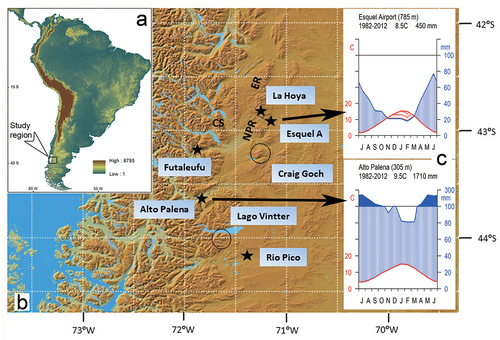
The two investigated mountain areas are located in northern Patagonia (Figures 1a, 1b). The first area, Craig Goch (Spanish: Sierra Colorada) is one of the isolated mountain massifs (43°13′ S; 71°17′ W) forming the Patagonides range (Patagonian Precordillera) to the East of the Lake Region Andes. It was named by Welsh immigrants who settled in the region more than 150 years ago. Maximum elevation in Craig Goch reaches c. 1,950 m. The second study area is located near Lago Palena/General Vintter (Winter), which straddles the Chile/Argentina border. For simplicity, we identify our study area directly to the South of the lake (almost exclusively) on the Argentinean side of the border as the Lago Vintter area. This area is located c. 90 km SSW of Craig Goch, on the eastern flank of the main range of the Andes (43°59′ S; 71°37′ W) and has a maximum elevation of c. 2,050 m. The lower limit of the study areas (1,400 m contour line) roughly corresponds to the Nothofagus treeline and delineates the mountain periglacial zone in the region.

Figure 1. (a) Study region in northern Patagonia (black rectangle); map downloaded from (Earth Explorer 2000) https://earthexplorer.usgs.gov/. (b) Location of the Craig Goch and Lago Vintter study areas (black circles), weather stations (black stars), and additional places of interest (ER = Esquel Range; NPR = Nahuel Pan Range; CS = Cerro Situaciòn); background downloaded from (Japan Aerospace Exploration Agency 2021) https://www.eorc.jaxa.jp/ALOS/en/aw3d30. (c) Simplified Walter and Lieth (1967) climate diagrams (R software, “climatol” package; Guijarro 2019) for Esquel Airport and Alto Palena; meteorological data from https://sv.climate-data.org/.

These mountain study areas are not strictly protected by law, but due to their remote location there is negligible human influence in the alpine vegetation belt. Small settlements are found in the foothills of both areas below 1,000 m elevation, with very occasional grazing of livestock (horses and cows) in the lower reaches of the Craig Goch area. No human impact was observed at any of the sampling points during fieldwork.

Bedrock in the Craig Goch (Sierra Colorada) mountain area is mainly composed of red-colored vulcanites of the Early Cenozoic Huitrera Formation (Haller et al. 2010). The main Andean range in the Lago Vintter study area consists of granitoids of the Cretaceous Rio Hielo Formation, with andesites, rhyolites, and tuff of the Jurassic La Plata Formation characterizing the eastern sector of the study area (Haller et al. 2010). In both areas there are glaciogenic deposits of Quaternary age, predominantly tills and sandurs from the last glaciation (Caldenius 1932; Haller et al. 2010).

The Late Quaternary glaciation history of both study areas is chronologically poorly constrained. Outlet glaciers of the Patagonian Ice Sheet were topographically confined to large valley systems North and South of the Craig Goch massif and to the Lago Vintter basin, with terminal moraines of Last Glacial Maximum age (25–21 ka) located just to the East of the mountain ranges (Davies et al. 2020; Leger et al. 2020). The Craig Goch and Lago Vintter study areas proper were likely not completely covered by glacier ice, with local cirque glaciers extending down-valley to coalesce with the large outlet glaciers of the Patagonian Ice Sheet. Following deglaciation, a series of neoglacial advances occurred during the Middle to Late Holocene. These have not been studied in detail in our study areas, but both to the north at 35° S (Espizua 2005) and to the south at 46° S (Aniya 1995) four neoglacial advances are recognized, dated between c. 6 ka and 0.5–0.2 ka (the latter corresponding to the Little Ice Age in the region). Glacial throughs are much more deeply incised in the Lago Vintter area, particularly in its western section, where steep bedrock characterizes the upper slopes of the glaciated area.

The most important climate normals (1982–2012) for selected stations in the study region are presented in Table 1 (localities are shown in Figure 1b). Simplified Walter and Lieth (1967) climate diagrams for Esquel Airport and Alto Palena are presented in Figure 1c.

Table 1. Location and climate normals of weather stations in the region of interest.

Weather station	Latitude	Longitude	Altitude (m)	MAAT (°C)	MTAP (mm)	PET > P
La Hoya (Argentina)	42°49.4′ S	71°15.3′ W	1,850	1.7	558^a	1 month^b
Esquel A (Argentina)	42°54.4′ S	71°08.8′ W	785	8.5	450	3 (to 5) months^c
Futaleufu (Chile)	43°11.1′ S	71°52.0′ W	355	9.5	2,014	None
Alto Palena (Chile)	43°37.1′ S	71°48.3′ W	305	9.5	1,710	None
Rio Pico (Argentina)	44°10.8′ S	71°22.2′ W	600	8.0	656	1 (to 2) months^d

Notes. Climate data from https://sv.climate-data.org (1982–2012) and https://www.snow-forecast.com/resorts/La-Hoya/history (2007–2018 MAAT bias adjusted to 1982–2012). MTAP = Mean total annual precipitation.

^aLa Hoya main station (1,525 m).

^bJanuary.

^c(November) December–February (March).

^dJanuary (February).

Climate in the main range of the Andes is classified as Cfb in the Köppen-Geiger classification system (Peel, Finlayson, and McMahon 2007). At low elevations (Futaleufu and Alto Palena), summers are warm and humid with potential evapotranspiration (PET) never exceeding precipitation (P). Localities to the East of the Andes have a Csb climate (Esquel Airport and Rio Pico), characterized by warm but drier summers with one to five months during which PET exceeds P. There are limited climate data from high-elevation sites. Approximate conditions can be calculated from meteorological observations at the ski resort La Hoya in the Esquel Range to the north of the Craig Goch massif (Figure 1b and Table 1). Mean annual air temperature (MAAT) at 1,850 m is c. 2.1°C for the period 2007–2018, which, based on records at Esquel Airport, is on average 0.4°C warmer than the 1982–2012 period. An altitudinal gradient of c. 0.64°C/100 m is obtained by comparing MAAT at Esquel Airport and La Hoya. From the records in Esquel Airport and Rio Pico (adjusted for elevation differences), a latitudinal gradient in MAAT of c. 1.1°C/100 km can be derived.

Longer term temperature and precipitation records are available from Esquel Airport (https://climexp.knmi.nl; Trouet and Van Oldenborgh 2013). There is no obvious trend in MAAT for the period of observation 1931–2018 (+0.007°C/decade), with only a very small overall decrease in mean total annual precipitation for the period 1896–2017 (−1.6 mm/decade). The longest record for southern South America is from Punta Arenas, Chile (53°09.4′ S; 70°54.6′ W; 37 m), extending from 1888 to 2018 (https://climexp.knmi.nl; Trouet and Van Oldenborgh 2013). There are slight decreases in both MAAT (−0.04°C/decade) and mean total annual precipitation (−2.6 mm/decade) over this time period. These observations concur with those reported for the region in the Fifth Assessment Report of the Intergovernmental Panel on Climate Change (Magrin et al. 2014).

The strong west to east precipitation gradient across the Andean mountain range has a significant effect on the altitude of the Equilibrium Line Altitude (ELA) of current glaciers in the study areas. At the latitude of Esquel, the ELA is modeled at c. 1,800 to 1,900 m altitude in the main range of the Andes but rises to >2,200 m in the Precordillera to the east (Condom et al. 2007). Currently in Craig Goch there are no glaciers, but in nearby areas on the eastern flank of the main range of the Andes there are small cirque glaciers with a predominantly southern to eastern aspect reaching from elevations of c. 2,200 m down to c. 1,800 m (Cerro Situación, CS in Figure 1b; Welsh name: Gorsedd y Cwmwl). In the Lago Vintter study area, located on the eastern flank of the main range of the Andes, small cirque glaciers reach down from elevations of c. 2,000 m to c. 1,650 m (southern aspect) and c. 1,750 m (eastern aspect).

No permafrost monitoring is ongoing in our study areas, but a statistical model has been developed to define permafrost distribution based on bottom temperature of snow cover measurements in the Esquel Range (ER in Figure 1b). According to Ruiz and Trombotto (2012), permafrost conditions are generally related to high altitude zones (>1,750 m) but can also be found locally at lower elevations in rock glaciers with a southern to eastern aspect due to the insulation provided by the rock debris cover and low incoming solar radiation. In the Patagonides at the latitude of Esquel, the ELA of glaciers at >2,200 m exceeds the elevation of the 0°C annual isotherm at c. 2,000 m (Condom et al. 2007), which favors the development of rock glaciers (Haeberli 1985). Permafrost in the Craig Goch area is largely restricted to rock glaciers. In the Lago Vintter study area, permafrost has been described from the highest mountain tops (C. Bianchi, pers. comm. 1998, cited in Trombotto 2000). A small rock glacier is putatively mapped in the southeastern part of the Lago Vintter study area, although this would need to be confirmed by direct field observation. In our study areas, permafrost can thus be considered of a sporadic nature only but locally extends down to 1,500 to 1,600 m elevation in rock glaciers. Rock glaciers and other periglacial landforms in the form of patterned ground and solifluction lobes and terraces have been described by Reato et al. (2017) at high elevations on the eastern flank of the Nahuel Pan Range, just north of the Craig Goch massif (NPR in Figure 1b).

There are no detailed descriptions of plant communities for our study areas. The treeline reaches up to c. 1,525 m in Craig Goch and c. 1,400 m in Lago Vintter and is formed in both cases by stunted (<5 m tall) deciduous Nothofagus antarctica trees. Mean annual air temperature of the warmest month (January) at the treeline near the station of La Hoya (1,525 m) is 10.3°C (1982–2012), which is similar to the values reported for many other alpine treelines in both the southern and northern Hemispheres (Cieraad, McGlone, and Huntley 2014). Above the treeline, plant cover depends on altitude and soil moisture gradients and is characterized by a mixture of dwarf shrubs, graminoids, and herbs. Cushion plants or mosses are co-dominant in wet meadows. Plant cover becomes sparse above 1,650 to 1,750 m in Craig Goch and c. 1,600 m in Lago Vintter.

Soils in our study areas are generally poorly developed, shallow, and stony, which is typical for high mountain environments. Detailed soil taxonomical studies are not available for the high mountain region of northern Patagonia. Pereyra and Bouza (2019) reported the presence of extensive areas with Andisols, but these are generally restricted to elevations below treeline and were not observed in our study areas. Cryogenic processes are active in the higher ranges of the mountains, as evidenced by the periglacial landforms observed in our study areas. Dominant soil orders (Soil Survey Staff 2014) are Entisols (Cryorthents in areas of shallow bedrock or coarse stony deposits and Cryaquents on glacio-fluvial outwash plains), Inceptisols (Cryocrepts and Haplumbrepts), and weakly developed Mollisols (e.g., Cryolls) in alpine grassland/dwarf shrub areas.

Methods

Field sampling

Fieldwork was carried out in January 2019 to coincide with the austral summer when weather conditions in the region are amenable. Based on preliminary land cover and landform maps derived from Google Earth (April 2009 and January 2010) and Sentinel 2B (February 2018) images, as well as field reconnaissance, transects between c. 0.5 and 2 km long were laid out that represent the altitudinal gradient, vegetation types, and landform features in the study areas. Three transects were established in Craig Goch (CG) and two in Lago Vintter (VT). Along each transect, either five (Craig Goch) or six (Lago Vintter) profile sites were identified with a handheld Global Positioning System (GPS) based on predefined strict distance (100 or 140 m) or altitude (50 or 100 m) interval criteria, in order to avoid any bias in exact site location. Placement of the transects depended on terrain conditions. Transects CG T1, CG T3, and VT T2 were straight lines on slopes with sampling sites at 140 m distance intervals (CG T1), 50 m elevation intervals (CG T3), and 100 m distance intervals (VT T2). Transects CG T2 and VT T1 first followed ridges and then continued into valleys, with sampling sites at 100 m elevation intervals (CG T2) and 50 m elevation intervals (VT T1). In total, twenty-seven soil profiles were described (twenty-six sampled) at elevations between 1,400 and 2,000 m. Even though all important vegetation types and landform features are represented in our data sets, soil profile collection preferentially targeted areas of plant cover and soil development, in order to obtain enough replication for SOC-rich sites. This bias is later removed in our upscaling approach.

Each profile site was photographed and a general description of topography (elevation, slope, and aspect), landform (and eventual periglacial features), and land cover was made. For the latter, a ground-truth plot with a radius of 5 m around the profile site was observed. We described the mean height of the uppermost vegetation stratum and the cover of plant functional types in all vegetation strata; that is, tree, dwarf shrub (<25 cm height), graminoids, ground layer (with herbs, cushion plants, mosses, and lichens), litter, water, bare mineral ground (grain size <4 cm), and large stones (grain size ≥4 cm). Because of overlapping strata, total cover can exceed 100 percent. At sites with sparse plant cover, profiles were dug in a vegetated patch of the 5-m-radius circle. In order to not overestimate SOC storage, the SOC content of the O–A–B horizons was weighed by the fraction vegetated area within the circle. For the remaining fraction of mineral bare ground, default SOC values from the collected BC/C horizons at the profile site were applied.

Soil pits were dug out with a spade for the full depth of soil development. Soil samples from the surface organic layer, if present, were cut out with a knife in the shape of a block, with careful measurement of dimensions to obtain volume. Deeper layers were collected by pushing or hammering a steel cylinder of known volume (100 cm³) into the exposed vertical pit wall at intervals of 4 to 10 cm depth. In most profiles, large stones (≥4 cm) were encountered and their percentage of volume for the depth interval represented by each collected soil sample was visually estimated. This approach introduces a degree of uncertainty that directly translates into the calculation of SOC stocks, because the volume fraction occupied by large stones is considered to hold no SOC. The original aim was to sample down to the standard depth of 100 cm, but this was only reached at one profile site (total depth 106 cm) due to shallow regolith or bedrock. Only about half of the profiles exceeded a depth of 30 cm. Evidence for the presence of permafrost in the form of ground ice was not encountered during sampling.

In total, 175 soil samples from twenty-six profile sites were collected. For each collected soil sample, data about soil texture and color, and occurrence of roots and small stones (<4 cm) were recorded. Another seven samples of large stones were taken to estimate the dry bulk density of the coarse fraction (CF). This allowed recalculating the weight fraction of small stones in soil samples into volume estimates. Two woody root samples were collected to measure their bulk density and carbon content in order to calculate their contribution to total C stock in the soil sample. Five samples of 1 to 3 cm depth intervals were specifically collected for radiocarbon dating. In total, ten samples from four soil profiles, representing topsoil organic, buried organic, and mineral subsoil layers, were selected for age determination.

Geochemical analyses

Soil samples (n = 175) were weighed before and after being dried at 60°C for 48 hours to calculate their water content (% weight) and dry bulk density (g cm⁻³). All samples were then homogenized and sieved through a 2-mm mesh and all stones (CF >2 mm) were weighed separately to measure the small stone fraction in the sample (% weight). For loss on ignition (LOI), the samples were again dried at 105°C and then burned at 550°C for 5 hours (LOI₅₅₀, % weight) to determine organic matter content. A selection of samples, representing different land cover classes, was burned at 950°C for 2 hours (LOI₉₅₀, % weight) to determine eventual carbonate content (Dean 1974; Heiri, Lotter, and Lemcke 2001). There was no evidence of carbonates in our samples, based on either the LOI₉₅₀ results or in the form of anomalous high C/N ratios in mineral subsoil samples (resulting from the additional contribution of inorganic C to total C in the sample). Subsamples from eighty-six samples of representative profiles were freeze-dried, kept in a desiccator, and then analyzed for their carbon (%C) and nitrogen (%N) contents and C/N (weight) ratio in an elemental analyzer (Carlo Erba NC2500) at the Department of Geological Sciences, Stockholm University. For the remaining samples (n = 89), a third-order polynomial regression (R² = 0.92; p < .05) was used to calculate the %C from the LOI data at 550°C, based on those samples for which both %C and LOI at 550°C values were available (Equation 1(1) $\begin{array}{rl}& \mathrm{\%}\mathrm{C}=-0.00007852{\left(\mathrm{\%}\mathrm{L}\mathrm{O}\mathrm{I}550\right)}^3+0.009806{\left(\mathrm{\%}\mathrm{L}\mathrm{O}\mathrm{I}550\right)}^2\\ & +0.1884\left(\mathrm{\%}\mathrm{L}\mathrm{O}\mathrm{I}550\right)\hspace{0.17em}.\end{array}$(1) ) ..

(1) $\begin{array}{rl}& \mathrm{\%}\mathrm{C}=-0.00007852{\left(\mathrm{\%}\mathrm{L}\mathrm{O}\mathrm{I}550\right)}^3+0.009806{\left(\mathrm{\%}\mathrm{L}\mathrm{O}\mathrm{I}550\right)}^2\\ & +0.1884\left(\mathrm{\%}\mathrm{L}\mathrm{O}\mathrm{I}550\right)\hspace{0.17em}.\end{array}$(1)

A polynomial fit was necessary in order to properly represent (and not overestimate) %C in mineral subsoil samples with low LOI₅₅₀ values (Figure A1).

Ten samples of bulk material (removing visible roots) were submitted for Accelerator Mass Spectrometry AMS ¹⁴C dating to the Radiocarbon Laboratory in Poznan, Poland. The resulting ages, in ¹⁴C yr BP, were calibrated to calendar years, cal yr BP (1950), using OxCal 4.4 (Bronk Ramsey 2009) and the Southern Hemisphere SHCal20 calibration curve (Hogg et al. 2020).

SOC stock calculations

The SOC storage (kg C m⁻²) for each sample (SOC_S) was calculated by multiplying the fraction of C by dry bulk density (g cm⁻³), depth interval (T), and 10 for unit conversion. Adjustments for coarse fragments were made, where CF_W is the weight fraction of small stones (>2 mm) in the samples and CF_V is the volume fraction of large stones (≥4 cm) described from the soil pits (Equation 2${\text{SOC}}_{\text{S}}\text{kg}\text{C}{\text{m}}^{\text{-2}}=\text{C}\times \text{DBD}\times 1-{\text{CF}}_{\text{W}}\times 1-{\text{CF}}_{\text{V}}\times \text{T}\times 10.(\text{2})$):

${\text{SOC}}_{\text{S}}\text{kg}\text{C}{\text{m}}^{\text{-2}}=\text{C}\times \text{DBD}\times 1-{\text{CF}}_{\text{W}}\times 1-{\text{CF}}_{\text{V}}\times \text{T}\times 10.(\text{2})$

The SOC mass was calculated for each individual sample and added up to a total SOC storage in the profile for the reference depths of 0 to 30 and 0 to 100 cm. Only one profile reached the depth of 100 cm. The underlying regolith or bedrock were assumed to contain a negligible amount of SOC. One profile site (VT T2-6), from bare ground near a perennial snow patch, was described in detail but not sampled. Default soil geochemical properties from a nearby similar site (VT T1-5) were used to estimate its SOC stock.

Land cover classification

Topography is based on a digital elevation model using ALOS PALSAR (2011) data, with a resolution of 12.5 m.

The land cover classification (LCC) of the two study areas was derived from a Sentinel 2B satellite image acquired the 15th of February 2018, with a resolution of 10 m (Copernicus Sentinel data 2019). In the final classification, we distinguish five different land cover classes: unvegetated terrain (including bedrock outcrops, block fields, water, perennial snow patches, and glacier ice), sparsely vegetated alpine, patchy vegetated alpine, densely vegetated alpine, and subalpine forest. A two-step procedure was applied in which first the upper forest belt, the alpine vegetation belt, and the high mountain barren zone were identified, followed by a second step in which the mosaiced alpine vegetation belt was further differentiated into sparse alpine, patchy alpine, and dense alpine.

For the first classification step, a maximum likelihood supervised classification (Jones and Vaughan 2010) was applied using the spectral bands 2–4 and 8 and the true color and false color images of the Sentinel 2B image. The training set consisted of twenty-five homogenous patches (>100 pixels) for each of the three land cover classes in each study area, which could easily be recognized from high resolution Google Earth imagery taken on 2009 and 2010 (Google Earth 2019) and photographs taken during fieldwork (2019). The accuracy and kappa index of this classification for each study area were calculated from a confusion matrix using a stratified random sampling scheme of an additional fifty points per land cover class. The second classification step, focusing on a subdivision within the alpine vegetation belt, was performed on the basis of vegetation indexes stacked with the true color image. The Normalized Difference Vegetation Index and the Soil Adjusted Vegetation Index both aim to distinguish the vegetation more clearly from the rest of the environment, with the Soil Adjusted Vegetation Index introducing a variable for reflectance of soil from in between the canopy and patches of vegetation (Huete 1988). The accuracy of this classification was checked against the land cover descriptions and photographs at the twenty-seven soil profile sites collected in the two study areas. In this regard, we should emphasize that it was not possible to link a specific profile site to a single 10-m pixel in the LCC due to the normal uncertainties in GPS measurements. Furthermore, mixed pixels occurred due to the highly mosaiced nature of the alpine vegetation. We used a kernel-3*3 approach to decide on the accuracy of the second classification step. The class assignment was considered accurate if a majority of nine pixels were correct. GPS estimates of elevation are particularly uncertain in mountain settings. We corrected elevation to values obtained from the Google Earth Pro terrain tool using the GPS geographic coordinate measurements.

Large-scale geomorphological features (glaciers, cirques, moraine ridges, nivation hollows, and rock glaciers) were mapped using Google Earth imagery (2009, 2010) and field observations (2019). Final topographic, land cover, and landform products were integrated in a geographic information systems environment (ArcMap 10.3, 2015).

SOC upscaling

The mean and standard deviation SOC storage for each land cover class was calculated based on all soil profiles assigned to that class. The SOC storage in the reference depths 0 to 30 and 0 to 100 cm was then weighed by the fraction of the combined study area covered by each land cover class and added for the total combined study area and the alpine vegetated area only (excluding bare ground and subalpine forest areas). In addition, proportions of area and total SOC storage per land cover class were computed for the Craig Goch and Lago Vintter areas separately. The mean and standard deviation total SOC storage were also calculated for the main landform classes in the combined study area, focusing on periglacial features.

Statistical methods

To derive error estimates for SOC storage in the combined study area, a spatially weighed 95 percent confidence interval (CI) was calculated following Thompson (1992). This CI was calculated to consider the relative spatial coverage, SOC storage variability, and degree of replication within each upscaling class (Equation 3(3) $CI=t\ast \sqrt{\sum (\frac{\left({a_i}^{2\ast }S{D_i}^2\right)}{n_i})},$(3) ):

(3) $CI=t\ast \sqrt{\sum (\frac{\left({a_i}^{2\ast }S{D_i}^2\right)}{n_i})},$(3)

where t is the upper α/2 of a normal distribution (t = 1.96), a_i is the fraction of the total combined study area per land cover class, SD_i is the standard deviation of the SOC storage per land cover class, and n_i is the number of replicates per land cover class. CI ranges presented here do not account for errors in the upscaling products (Hugelius 2012).

Relationships between geochemical variables, plant cover, soil attributes, and topography (elevation) were statistically analyzed with the Microsoft Excel 2010 and PAST 3 (Hammer, Harper, and Ryan 2001) software packages. Regressions were considered significant if p < .05.

Results

Maps of the study areas

The CG and VT study areas each cover an area of c. 36 km², resulting in a combined total area of c. 72 km². Their lower limit is placed at the 1,400 m contour line, with the exception of the southwestern corner of the Lago Vintter area, where the limit cuts through a mountain saddle reaching c. 1,700 m in elevation.

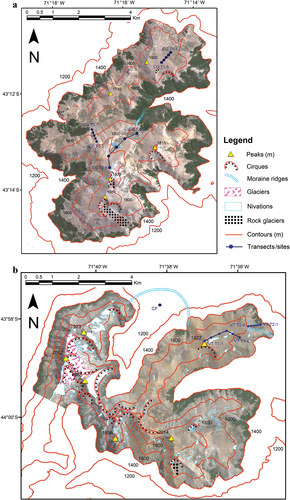
Figures 2a and 2b depict large-scale glacial and periglacial landscape features as well as the main vegetation belts in the Craig Goch and Lago Vintter study areas, respectively. The background represents the true color image of the 2018 Sentinel 2B satellite image, depicting the upper Andean Nothofagus forests in dark green, vegetated alpine areas in pale green, and bare ground in grey/brown. At this scale it is not possible to map small periglacial features such as patterned ground (sorted circles, stripes) and solifluction lobes and terraces, or distinguish between alpine vegetated areas with different plant cover densities. In the final land cover classification, the alpine vegetation belt was further subdivided into areas of dense, patchy, and sparse plant cover (see below).

Figure 2. (a) Map of the Craig Goch study area showing topography (peaks and contour lines), large-scale landform features (cirques, moraine ridges, rock glaciers, nivation hollows), land cover (true color image background), and location of transects and sampled profiles. The legend unit “Glaciers” only applies to the Lago Vintter study area (see Figure 2b). (b) Map of the Lago Vintter study area showing topography (peaks and contour lines), large-scale landform features (glaciers, cirques, moraine ridges, rock glaciers, nivation hollows), land cover (true color image background), and location of transects and sampled profiles. The mountaintop (1,822 m) near site VT T1-1 is locally known as “Peak Gretel.” Site CF stands for Cors Fochno (Fochno Bog), a large peatland area located at 1,010 m elevation, characterized by a 233-cm peat deposit underlain by 210-cm (glacio-) fluvial and lacustrine deposits. For legend, see Figure 2a.

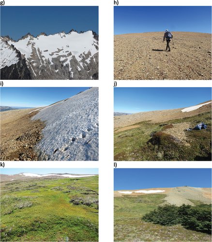
Figures 3a to 3f and Figures 3g to 3l show examples of land cover classes and landform types in the Craig Goch and Lago Vintter study areas, respectively.

Figure 3. (a)–(f) Examples of land cover classes and landform types in Craig Goch: (a) bare ground on frost-shattered bedrock and a small rock glacier (c. 1,800–1,900 m); (b) sparse alpine vegetation on large stripes, site CG T3-5 (c. 1,700 m); (c) sparse alpine vegetation in area with small solifluction lobes, site CG T1-4 (c. 1,690 m); (d) dense alpine vegetation on outwash plain with terminal moraine in the background, site CG T2-3 (c. 1,750 m); (e) dense alpine vegetation on stabilized solifluction slope with bare area, site CG T1-1 (c. 1,625 m); (f) patch of Nothofagus forest, site CG T3-1, patchy and sparse alpine vegetation, sites CG T3-2 to T3-4, on colluvium slope (c. 1,500–1,650 m).

Figure 3. Continued. (g)–(l) Examples of land cover classes and landform types in Lago Vintter: (g) glaciers and steep bedrock (c.1,700–2,000 m); (h) bare ground on small stripes, site VT T1-2 (c. 1,750 m); (i) bare ground and nivation hollow, site VT T2-6 (c. 1,550 m);(j) dense alpine vegetation with bare area on solifluction terrace, near site VT T2-5 (c. 1,515 m); (k) dense alpine vegetation on stabilized solifluction slope, site VT T1-6 (c. 1,550 m); (l) patch of Nothofagus forest on colluvium, site VT T2-1, with alpine vegetation and nivation hollow in the background, sites VT T2-2 to T2-6, and lateral moraine to the right (c. 1,400–1,550 m).

The land cover classification

The first step in the LCC to distinguish between forest, alpine vegetation, and bare ground had an accuracy and kappa index of classification of 0.89 and 0.83, respectively, for the Craig Goch study area. The same parameters for Lago Vintter are 0.95 and 0.92, respectively.

In the second step to distinguish between dense, patchy, and sparse alpine vegetation, twenty-one out of twenty-seven sites were appropriately classified according to the kernel-3*3 approach. Misclassifications can be expected due to the highly fragmented character of plant cover in the alpine belt, with the three plant cover density classes alternating at fine spatial scales (see, e.g., Figures 3b–3e, 3j).

The LCC was used to group soil profile sites into land cover classes for upscaling of SOC stocks to the full Craig Goch and Lago Vintter study areas. Individual sites were also grouped according to landform criteria. It was not possible, however, to map the spatial extent of some of the fine-scale periglacial landforms (e.g., patterned ground, solifluction features) due to relatively large study areas and the 10-m resolution of the satellite image. Hence, no spatial upscaling of SOC stocks was performed based on geomorphological criteria.

Soil profile descriptions

Metadata regarding the twenty-seven described soil profile sites, including geographic coordinates, topographic data, land cover class and landform type, soil attributes, and plant functional type cover, are presented in Table A1. Figures 4a and 4b present a selection of four soil profiles from the CG and VT study areas, respectively, representing main land cover classes and landform types and ranges of SOC storage. The following geochemical parameters are included: volume of large (≥4 cm) and small (>2 mm – <4 cm) stones, water loss (% weight), dry bulk density (g cm⁻³), carbon content (% weight), and C/N (ratio). Depths of dated horizons are indicated with black crosses (see Table 2).

Table 2. Radiocarbon dates of selected soil samples reported as ¹⁴C ages and calibrated ages.

Poznan LabNumber	Landform	Profile	Depth (cm)	Horizon type	Submitted material	Age ^14C yr BP	Age cal yr BP^a(modern)
Poz-112716	Stabilized solifluction	VT T1-6	14–16	Base top organics	Bulk	111.33 ± 0.32 pMC	Modern
Poz-119022	Stabilized solifluction	CG T1-1	30–36	B-horizon	Bulk	635 ± 30	614, 556
Poz-119023	Stabilized solifluction	CG T1-2	22–28	B-horizon	Bulk	1680 ± 30	1550, 1489
Poz-119026	Solifluction terrace	VT T2-4	29–35	Base top organics	Bulk	1130 ± 30	971, 1037, 939
Poz-112717	Solifluction terrace	VT T2-4	57–59	Buried organics	Bulk	395 ± 30	465, 348
Poz-112718	Solifluction terrace	VT T2-4	76–78	Buried organics	Bulk	1180 ± 30	1005, 1055
Poz-112719	Solifluction terrace	VT T2-4	101–104	Buried organics	Bulk	1785 ± 30	1658, 1695
Poz-119024	Outwash plain	CG T2-3	12–18	Upper top organics	Bulk	200 ± 30	196, 267, 148
Poz-119025	Outwash plain	CG T2-3	25–27	Middle top organics	Bulk	107.29 ± 0.29 pMC	Modern
Poz-112715	Outwash plain	CG T2-3	38–39	Base top organics	Bulk	1700 ± 30	1559

Note. ^aMean of 68.3 percentage ranges in decreasing order of probability (highest probability age in bold).

Figure 4. (a) Geochemical properties of selected soil profiles from the Craig Goch study area indicating land cover class, landform type, altitude, and total SOC storage. Depths of dated horizons are indicated with black crosses in the %C and C/N panel to the right.

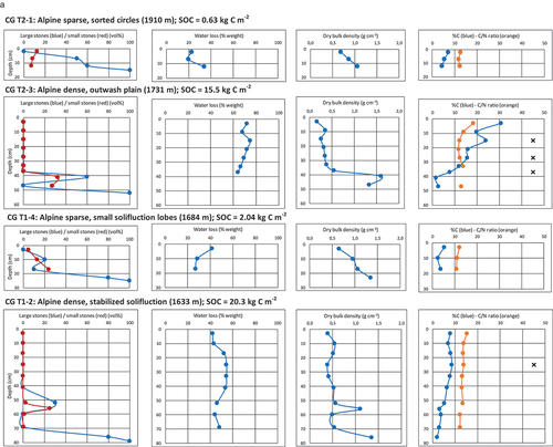
Figure 4. Continued. (b) Geochemical properties of selected soil profiles from the Lago Vintter study area indicating land cover class, landform type, altitude,and total SOC storage. Depths of dated horizons are indicated with black crosses in the %C and C/N panel to the right.

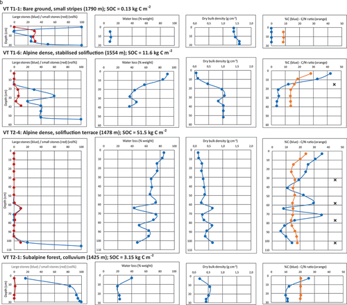
Low SOC storages are found at the highest elevations in areas with no or sparse vegetation. Profile sites VT T1-1 (1,790 m) and CG T2-1 (1,910 m) feature stone pavements on their surface, with small stripes and poorly sorted circles (Figures 4a, 4b, respectively). Soils are very shallow (≤20 cm) and stony. Soil moisture is low, dry bulk density is high, and %C and C/N are low. Lowest SOC storage of all collected soil profiles was calculated for the VT T1-1 site with only 0.13 kg C m⁻². This site is completely devoid of any plant cover. It has a surface pavement of large stones arranged in stripes, followed by a c. 15 cm horizon of much finer mineral subsoil, overlying regolith. Site CG T2-1 has the lowest SOC storage of profiles in the Craig Goch area, with 0.63 kg C m⁻². Slightly higher SOC stocks are encountered in Craig Goch at medium to high-elevation sites with sparse vegetation featuring small solifluction lobes. For example, site CG T1-4 (1,684 m) has a slightly deeper (25 cm) soil profile but otherwise similar characteristics to VT T1-1 and CG T2-1, resulting in an SOC storage of 2.04 kg C m⁻² (Figure 4a).

Highest SOC storages were found in alpine areas with dense land cover on solifluction terraces and solifluction slopes that have been stabilized by vegetation. These sites have variable but generally greater soil depths, low to medium stone contents, high soil moisture, low to moderate dry bulk density, and moderate to high %C and C/N. Highest total SOC storage (51.5 kg C m⁻²) of all collected soil profiles was recorded for the 106-cm-deep VT T2-4 solifluction terrace site (1,478 m), in which multiple buried organic layers were encountered (Figure 4b). This is the only site in which total SOC stock exceeded its SOC 0–100 cm stock (49.7 kg C m⁻²). SOC storage in solifluction terraces is highly variable depending on solifluction feature and profile location within it and was as low as 6.00 kg C m⁻² at site VT T2-3 (1,451 m; not shown). This profile from the flat top of a small solifluction terrace, with 8 percent stones at the surface, was only 21 cm deep. Sites on slopes with stabilized solifuction had relatively high SOC storage, varying between 11.6 kg C m⁻² at site VT T1-6 (1,554 m) and 20.3 kg C m⁻² at site CG T1-2 (1,633 m). The latter profile had the highest recorded SOC storage in the Craig Goch area (Figures 4a–4b).

Flat outwash plains occupy very small areas delimited by moraine ridges and can have dense land cover. Site CG T2-3 (1,731 m) has a wetland character with cushion plants and small ponds, with a c. 38-cm peaty surface layer and an SOC storage of 15.5 kg C m⁻² (Figure 4a). A profile from a similar setting in the Lago Vintter area had an SOC storage of 14.8 kg C m⁻² (VT T2-2, 1,435 m, not shown).

The stabilized solifluction sites CG T1-2 and VT T1-6, as well as the outwash plain site CG T2-3, have in common that the upper and middle SOC-rich soil horizons are underlain by a stone layer, followed by a 10- to 30-cm horizon of much finer mineral subsoil, overlying regolith. This lower part of the sequence resembles the profile described for the bare ground VT 1-1 site (Figures 4a–4b).

Slopes with colluvium are found across the elevational gradient in both study areas. Plant cover is normally sparse to patchy alpine, or dwarf forest. Soil profiles are shallow, stony and dry, with relatively low SOC storage. An example is site VT T2-1 (1,425 m), in the uppermost Nothofagus dwarf forest of the Lago Vintter area, with an SOC storage of 3.15 kg C m⁻² (Figure 4b).

We observed significant relationships between plant cover and soil depth with SOC storage considering all profiles in both study areas (Figures A2a–A2b). Similarly, significant relationships were found between C content and C density with soil moisture considering the individual samples from all profiles in both study areas (Figures A2c–A2d).

Radiocarbon dating

Calibrated radiocarbon ages from ten samples are presented in Table 2. Dating focused on deep and SOC-rich profiles in solifluction features and peat(y) deposits in an outwash plain. All sites had a dense alpine plant cover.

The dense vegetation on a stabilized solifluction slope at site VT T1-6 had a wetland character with grass–herb–moss vegetation (and small water pools). The base of the 16-cm-deep upper peat(y) layer was modern in age. Dates of the B-horizons of relatively well-developed soils in dense (dwarf shrub)–grassland vegetation on stabilized solifluction slopes at sites CG T1-1 (30–36 cm) and CG T1-2 (22–28 cm) yielded highest probability ages of 614 and 1550 cal yr BP, respectively.

Multiple dates are available from the 106-cm-deep soil profile VT T2-4 exposed in the frontal riser of a solifluction terrace. The site has a dense (dwarf shrub)–grassland–moss vegetation and is characterized by a peat(y) surface layer and multiple buried organic layers. The deepest buried C-enriched layer (101–104 cm) has a highest probability age of 1658 cal yr BP, which is the oldest of all of our dated samples. This date provides a minimum age for the lateral moraines delimiting the area of transect VT T2. The basal part of the upper peat(y) layer (29–35 cm) in this solifluction profile has a highest probability age of 971 cal yr BP. Two other buried C-enriched samples at intermediate depths of 57 to 59 cm and 76 to 78 cm showed the highest probability ages of 465 and 1005 cal yr BP, respectively. The age at 57 to 59 cm is younger than the basal age of the upper peat(y) layer, indicating a mixing of soil layers in this solifluction terrace.

Site CG T2-3 in an outwash plain has a wetland character with a dense (dwarf shrub)–grassland–cushion vegetation (with some water pools and nearby patches of bare ground on the active floodplain). The upper peat(y) deposit has a basal age of 1559 cal yr BP (38–39 cm) and very young ages at intermediate and upper levels. The basal age provides a minimum age for the terminal moraines delimiting the outwash plain.

SOC upscaling

The number of sites for each recognized land cover class, their proportional area representation in the combined Craig Goch and Lago Vintter study areas and the alpine vegetation belt only, and statistics concerning their elevation, plant cover, soil depth, and SOC 0–30 and 0–100 cm storages are summarized in Table 3.

Table 3. Attributes and SOC storage (kg C m⁻²) for each land cover class (mean and standard deviation) and weighed SOC storage (kg C m⁻²) considering proportional representation of land cover classes for Craig Goch and Lago Vintter combined total study area and for alpine vegetated area only (mean and confidence interval).

Land cover class	Sites (n)	Proportion study areas (%)	Proportion alpine vegetated (%)	Elevation range of sites (m)	Plant cover (%)	Soil depth (cm)	SOC 0-30cm (kg C m^−2)	SOC 0-100cm (kg C m^−2)
Subalpine forest	2	14.9		1468 ± 62	70 ± 7	28 ± 3	5.34 ± 3.11	5.34 ± 3.11
Dense alpine	7	3.1	19.2	1567 ± 102	87 ± 17	66 ± 23	11.0 ± 2.52	20.9 ± 13.0
Patchy alpine	5	4.8	29.6	1559 ± 80	40 ± 29	41 ± 18	5.36 ± 1.73	6.86 ± 3.15
Sparse alpine	8	8.3	51.2	1717 ± 101	12 ± 5	29 ± 11	1.61 ± 0.87	1.80 ± 1.01
Bare ground	5	68.9		1680 ± 98	0 ± 0	26 ± 8	0.55 ± 0.55	0.56 ± 0.54
Total study area	27	100			16	28	1.91 ± 0.73	2.31 ± 0.79
Alpine vegetated	20	16.2	100		35	40	4.52 ± 0.65	6.96 ± 2.05

The mean SOC storage of the combined total study area including all vegetated land cover classes as well as the considerable proportion of bare ground areas is 1.91 ± 0.73 kg C m⁻² for the 0–30 cm and 2.31 ± 0.79 kg C m⁻² for the 0–100 cm soil depth intervals. The top 30 cm of soil thus holds, on average, 82.6 percent of the total soil stocks. If we only consider alpine vegetated areas, which represent 16.2 percent of the total combined study area, SOC storage values are higher; that is, 4.52 ± 0.65 kg C m⁻² (0–30 cm) and 6.96 ± 2.05 kg C m⁻² (0–100 cm). The alpine belt corresponds to the periglacial zone, which includes areas of dense plant cover with deep and SOC-rich profiles in solifluction features (and highly localized outwash plains). The dense land cover class has the highest SOC 0–100 cm storage with 20.9 ± 13.0 kg C m⁻² but only represents 3.1 percent of the total combined study area and 19.2 percent of the vegetated alpine belt. The lowest mean SOC 0–100 cm storage with 0.56 ± 0.54 kg C m⁻² is found in the bare ground class, which occupies 68.9 percent of the total combined study area (Table 3).

Figures 5a and 5b present proportional contribution of each land cover class to surface area and to SOC 0–100 cm storage for the Craig Goch and Lago Vintter study areas separately. Site replication is very low in a few cases and the mean value for bare ground from Lago Vintter is adopted as a default value for the same class in Craig Goch. Field observations of bare areas in Craig Goch (Figure 3a) confirmed that uncertainties related to the use of the Lago Vintter default value were minimal. Site replication in both study areas was better for the important SOC-rich dense alpine class.

Figure 5. Proportional contribution to area (blue) and SOC 0–100 cm storage (orange) of each land cover class in the (a) Craig Goch and (b) Lago Vintter study areas.

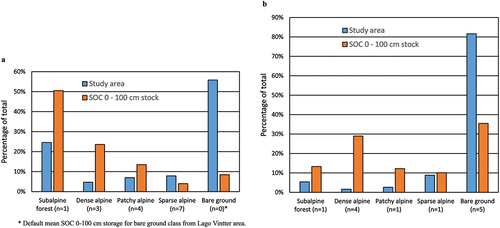
Overall patterns among land cover classes are quite similar between study areas. In both cases, the dense alpine class occupies the lowest proportion of surface area but has a very high relative contribution to SOC 0–100 cm storage. In contrast, the bare ground class has the largest surface area proportions but (very) low relative contributions to SOC 0–100 cm storage. There are also some marked differences between study areas. The class subalpine dwarf forest occupies a much larger proportion of area in Craig Goch (25 percent) compared to Lago Vintter (5 percent). The lower limit of both study areas is the 1,400 m contour line, but the Nothofagus treeline is located at a higher elevation in the Craig Goch area (c. 1,525 m) than in the Lago Vintter area (c. 1,400 m) due to its lower latitude location. In addition, the dwarf forest soil profile collected in Craig Goch is more SOC-rich (CG T3-1, 7.53 kg C m⁻²) than the Lago Vintter site (VT T2-1, 3.16 kg C m⁻²), but this difference might not necessarily hold with greater site replication in each study area. The class bare ground occupies a much larger area in Lago Vintter (82 percent) than in Craig Goch (56 percent) due to its more southern location and its slightly higher maximum elevation and more deeply incised valleys with an abundance of steep bedrock slopes (Figure 3g). There are only small differences in mean SOC 0–100 cm storage between Craig Goch and Lago Vintter for the dense alpine (18.4 versus 22.7 kg C m⁻²), patchy alpine (7.08 versus 6.00 kg C m⁻²), and sparse alpine (1.85 versus 1.46 kg C m⁻²) land cover classes, although the dense and patchy classes occupy a somewhat larger proportion of area in Craig Goch. As a result of these differences, mean SOC 0–100 cm storage is somewhat higher in Craig Goch (3.67 kg C m⁻²) compared to Lago Vintter (1.27 kg C m⁻²).

We also assessed SOC storage as a function of landform (Table 4). This approach yields important information regarding the effect of periglacial processes on soil development and SOC storage in the alpine vegetation belt but could not be used for scaling purposes due to the lack of high-resolution geomorphological maps for the study areas.

Table 4. Attributes and mean and standard deviation of total SOC storage (kg C m⁻²) for the full depth of soil profiles for different landform types in the Craig Goch and Lago Vintter combined study area.

Landform classes	Number of sites	Elevation range (m)	Slope (°)	Plant cover (%)	Large stones (%)	Soil depth (cm)	Total SOC (kg C m^−2)
Sorted circles	2	1,809 ± 144	8 ± 4	9 ± 0	33 ± 25	19 ± 6	1.37 ± 1.33
Small stripes	3	1,746 ± 43	10 ± 2	0 ± 0	22 ± 12	29 ± 8	0.21 ± 0.07
Large stripes	1	1,704	30	8	80	25	0.71
Nivations	2	1,580 ± 40	17 ± 12	0 ± 0	10 ± 0	22 ± 9	1.08 ± 0.49
Small solifluction lobes	3	1,719 ± 92	13 ± 3	14 ± 4	22 ± 3	34 ± 9	3.74 ± 2.59
Solifluction terraces	5	1,517 ± 65	16 ± 6	78 ± 25	4 ± 4	60 ± 31	18.3 ± 18.8
Stabilized solifluction	3	1,604 ± 43	9 ± 1	83 ± 22	3 ± 3	69 ± 18	17.1 ± 4.80
Outwash plains	2	1,583 ± 209	3 ± 2	80 ± 21	8 ± 11	48 ± 6	15.2 ± 0.44
Colluvium	6	1,566 ± 88	13 ± 7	37 ± 29	11 ± 11	31 ± 9	3.21 ± 2.32

Note. Large stones have grain size ≥4 cm.

Highest total SOC storages (full soil depth) of 17.1 to 18.3 kg C m⁻² were found in stabilized solifluction slopes (Figures 3e, 3k) and solifluction terraces (Figure 3j). Both of these landforms normally have a high plant cover and deep soil profiles, although water pools and/or stony bare ground patches may occur. High mean SOC stocks (15.2 kg C m⁻²) are also present in flat outwash plains (Figure 3d). Lowest mean SOC storages of <1.5 kg C m⁻² correspond to high alpine patterned ground sites such as sorted circles and (small and large) stripes as well as nivation hollows, which all have low plant cover and shallow soils. Sorted circles are generally poorly developed and have a variable diameter of c. 30–200 cm. Lineations of coarser stones in small stripes are generally c. 30 cm apart (Figure 3h), whereas the large stripe site has an elongated area of patchy plant cover and soil development <1 m wide, separated by stone fields of c. 2 m width (Figure 3b). Nivation hollows are found from mid- to high elevations and have a distinct eastern to southern aspect (Figure 3i). Sites in areas with small solifluction lobes (Figure 3c) and on slopes with colluvium (Figures 3f, 3l) have intermediate characteristics, with total SOC storage of 3 to 4 kg C m⁻² (Table 4).

Altitudinal gradients

Figures 6a to 6d depict the elevational gradients in our study areas. The altitudinal range of mapped large-scale glacial and periglacial landforms (glaciers and rock glaciers), as well as observed smaller periglacial landscape features (patterned ground, solifluction lobes and terraces, nivation hollows), on or in the immediate vicinity of the transects are shown in Figures 6a and 6d for Craig Goch and Lago Vintter, respectively. Figures 6b and 6c compare the observed plant cover and total SOC storage at profiles sites as a function of elevation in both study areas. Logarithmic regressions are significant (p < .05) except for SOC 0–100 cm storage versus elevation in the Craig Goch area, which is nearly significant (p ≈ .08). These regressions explain much more of the observed variability in Lago Vintter (plant cover R² = 0.62 and SOC R² = 0.70) compared to Craig Goch (plant cover R² = 0.34 and SOC R² = 0.22).

Figure 6. Schematic representation of glacial and periglacial landforms in Craig Goch (a) and Lago Vintter (d) and comparison of plant cover (b) and SOC storage (c) between study areas as a function of elevation.

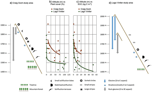
Overall, there is a 100- to 150-m elevation difference in plant cover and SOC storage trends between study areas, which mirrors the higher treeline in Craig Goch (c. 1,525 m) compared to Lago Vintter (c. 1,400 m). The Craig Goch study area displays a large range in plant cover and SOC storage at mid- to low elevations, which can be explained by topographic characteristics. The lower parts of transects T1 and T2, sites CG T1-1, T1-2, T2-4, and T2-5 (1,521–1,650 m), are located on concave slopes, which results in generally higher soil moisture, the development of solifluction features, and thicker soils. These sites have generally a denser plant cover (45–71 percent) and higher SOC storage (7.88–20.3 kg C m⁻²). In contrast, the two lower alpine sites on transect T3, sites CG T3-2 and T3-3 (1,512–1,604 m), are located on a convex slope, with shallow, stony, and dry soils in colluvium with a sparser plant cover (18–46 percent) and lower SOC storage (1.08–2.52 kg C m⁻²). In addition, the Craig Goch study area has a clear outlier in the mid-elevation flat outwash plain (site CG T2-3, 1,731 m; Figure 3d), with dense plant cover (65 percent) and high SOC stocks (15.5 kg C m⁻²). These results point to the importance of local edaphic conditions on top of elevational criteria for the degree of plant cover and size of SOC stocks at sites.

The Lago Vintter area shows a much stronger trend with elevation, even though alpine sites (e.g., VT T2-3) with relatively low SOC stocks (6.00 kg C m⁻²) are reported from lower altitudes (1,451 m). The Nothofagus sites in both study areas (CG T3-1 and VT T2-1) have shallow soils developed in dry colluvium slopes with average SOC stocks (3.15–7.54 kg C m⁻²). No periglacial processes were observed in the subalpine forest belt. Hence, the highest SOC stocks in our study areas were found in solifluction features of the alpine vegetation belt.

Discussion

Mountain permafrost in our study areas is restricted to rock glaciers and the highest mountaintops in Lago Vintter, which do not have any plant cover and soil development and hold no SOC stocks. We documented very low SOC stocks in patterned ground at high elevation, even though these sites often have a c. 10 to 30 cm fine-grained mineral horizon directly under the stone pavement that is potentially suitable for vegetation establishment. An example is site VT T1-1 (0.13 kg C m⁻²), which is currently completely devoid of plant cover and has extremely low (0.14–0.17) %C values in the soil profile.

Most soils in the alpine vegetation belt are shallow and stony, but periglacial processes such as solifluction can result in deeper soils and higher SOC storage. Highest mean SOC stocks were found in solifluction terraces (18.3 kg C m⁻²) and stabilized solifluction slopes (17.1 kg C m⁻²). There was, however, great variability in SOC storage among and within solifluction features (range = 6.00–51.5 kg C m⁻²). Solifluction can lead to a mixing and burial of organic layers, as shown by site VT T2-4 with inverted age sequences. It also shows that deep SOC can be preserved in the absence of permafrost as a result of burial in a cold periglacial environment. The contribution of solifluction features to mean SOC storage for the entire combined study area is still limited due to the restricted distribution of these SOC hotspots in the periglacial mountain environment.

Whereas there is a clear altitudinal gradient of decreasing SOC with increasing elevation in both areas, edaphic conditions and catenary position play a key role in promoting SOC storage. Sites located in flat basins (CG T2-3) and concave depressions (e.g., CG T1-2, VT T1-6) tended to show high soil moisture levels, which were significantly correlated to high %C and C density values in the soil matrix.

All dated samples in this study are younger than 1700 cal yr BP. Oldest basal ages at sites CG T2-3 (1559 cal yr BP) and VT T2-4 (1658 cal yr BP) provide a minimum age for the terminal and lateral moraines delimiting these areas (Figures 3d, 3l). We propose a neoglacial age for the glacier advances associated with the formation of these moraines. Of interest are also the buried stone pavements at sites CG T1-2, CG T2-3, and VT T1-6, which resemble the current profile at the high alpine VT T1-1 site. A date of 1550 cal yr BP of the overlying B-horizon at site CG T1-2 also suggests a possible neoglacial age for these paleo-surfaces that could be associated with a colder climate prevailing at the time.

Mean and range of SOC 0–100 cm storage in our northern Patagonia mountain study areas at latitude 43°–44° S can be compared to a recent study in the high mountain environment of the Veguitas catchment in the semi-arid Central Andes at latitude 33° S (Kuhry et al. in press). Our mean SOC storage of 2.31 kg C m⁻² is higher than the 0.33 kg C m⁻² reported for the Veguitas study area, which encompasses a much greater elevational range from 3,000 to 5,500 m. The vegetation limit in the Veguitas area is located at c. 3,600 m and, as a result, only 8 percent of the study area has plant cover and soil development, compared to 31 percent in our combined Patagonia study areas. Nonetheless, even when comparing the vegetated portions of both study areas, the alpine vegetation belt in our Patagonia areas has a higher mean SOC storage (6.96 kg C m⁻²) than the Veguitas vegetated area (3.62 kg C m⁻²). The SOC hotspot in Veguitas is a 102-cm-deep peat profile on an outwash plain holding 53.1 kg C m⁻², similar in magnitude to the maximum SOC stock of 51.5 kg C m⁻² in the 106-cm-deep solifluction terrace VT T2-4 profile observed in this study. However, peat(y) soils in the Veguitas area had a minimal coverage of only 1.36 percent of the vegetated area, similar to the highly localized outwash plain areas documented in this study. Solifluction features occupy c. 30 to 40 percent of the vegetated alpine belt in the Patagonian areas (largely overlapping with the dense land cover class and partly with the patchy land cover class) but were not observed in the vegetated parts of the Veguitas area (Kuhry et al. in press). The wetter climate of northern Patagonia also promotes higher soil moisture levels in favorable topographic settings, which are linked to higher soil C density values.

Similar transitions with elevation in plant cover and periglacial landforms to those observed in northern Patagonian mountains have been described by Hastenrath (1971) for the Cordillera Real of Bolivia (16° S) but at a much higher altitudinal range between 4,400 and 5,400 m. This area is located in the transition to the more humid mountain regions of the subtropical and tropical Andes. The treeline on the eastern slopes of the range is located at c. 3,500 m. A zone of “bound” solifluction landforms, including terraces, was reported between 4,400 and 5,000 m, the latter altitude corresponding with the upper limit of extensive plant cover in the area. Above this elevation, a zone with patterned ground (sorted circles, stripes, and stone pavements) is present. No soil or SOC data are available from the area. Zimmermann et al. (2010) provided total SOC stocks down to bedrock for the mountain cloud forest to alpine puna transition (3,000–3,900 m) in the Peruvian Andes (13° S), with mean values for forest, shrub transition zone, and grass puna ranging between 11.8 and 14.7 kg C m⁻². This study area is located well below the permafrost/periglacial zone in the region.

Landscape-level studies of SOC storage that use similar fieldwork and upscaling approaches as in this study and consider the negligible contribution to mean SOC storage of extensive bare ground areas typical of mountain settings have been carried out in the Northern Hemisphere permafrost zone. Fuchs, Kuhry, and Hugelius (2015) reported that the high alpine Tarfala valley (500–2,100 m), in the Scandes Mountains of northern Sweden, has a mean SOC 0–100 cm storage of 0.9 kg C m⁻² for total study area and 4.6 kg C m⁻² for vegetated area only. There is very limited overlap between the upper vegetation belt and the mountain permafrost zone. As a consequence, negligible amounts of SOC are stored in permafrost. The upper reaches of Aktru valley (2,100–4,000 m), in the High Altai of Central Asia, have a mean SOC 0–100 cm storage of 0.9 kg C m⁻² for total study area and 3.1 kg C m⁻² for vegetated area only (adapted from Pascual, Kuhry, and Raudina 2020). Even though the Aktru area is located in continuous permafrost terrain, negligible amounts of SOC are stored in the permafrost layer due to deep active layers characteristic of mountain settings (Bockheim and Munroe 2014). Wojcik et al. (2019) reported values of 1.0 kg C m⁻² for the total study area and 4.2 kg C m⁻² for vegetated area only for a high Arctic mountainous area on Brøgger Peninsula (0–900 m), Svalbard. Highest mean SOC 0–100 cm stocks of 6.7 kg C m⁻² were observed in the class “solifuction slopes.” Even though Brøgger Peninsula is located in the continuous permafrost zone, negligible SOC stocks are found in the permafrost layer.

The five mountain areas with detailed SOC inventories discussed above have in common that mean SOC storage is significantly reduced due to the high proportion of bare ground areas. The vegetated areas account for only 8 percent (Veguitas, Central Andes), 18 percent (Brøgger Peninsula, Svalbard), 19 percent (Aktru, Altai), 27 percent (Tarfala, Scandes), and 31 percent (Craig Goch and Lago Vintter, Patagonia) of the total study areas. The weighted landscape-level mean SOC storage range of 0.3 to 2.3 kg C m⁻² for these study areas is much lower than the mean SOC storage of 15.2 kg C m⁻² for worldwide mountain permafrost soils given in the review by Bockheim and Munroe (2014). The latter study focused on vegetated areas of the mountain permafrost zone, but the reported mean SOC storage is still much higher than the range of 3.1 to 7.0 kg C m⁻² for vegetated areas in the five detailed mountain SOC inventories. Regional and local differences in SOC storage in mountain settings is highly likely, with areas of solifluction, alluviation, and paludification creating hotspots of SOC storage in an otherwise low-SOC environment. Nonetheless, a global appraisal of SOC stocks in mountain permafrost/periglacial settings that considers the role of large portions of the landscape occupied by bare ground with negligible SOC stocks is advisable.

The low mean SOC storage in mountain settings stand in strong contrast with very SOC-rich lowland areas in the northern permafrost region, where total SOC storage is often an order of magnitude higher due to deep cryoturbated soils, peat deposits, and loess sequences (Tarnocai et al. 2009; Hugelius et al. 2014). There is considerable concern that permafrost thaw and collapse in these northern areas will result in a significant remobilization of SOC stocks and the subsequent release of greenhouse gases to the atmosphere that will exacerbate global warming (Kuhry et al. 2010; Schuur et al. 2015; Turetsky et al. 2020). This C release from permafrost soils is expected to exceed an increased C uptake in phytomass due to a northward shift of high latitude vegetation zones (Abbott et al. 2016).

The northern Patagonian mountain region is projected to experience warming of up to c. 3°C similar to the global average under Representative Concentration Pathway 8.5 by the end of this century, with possibly very limited decreases in precipitation (Magrin et al. 2014). Using the calculated 0.64°C/100 m elevational lapse rate calculated for the northern Patagonian mountains, this warming would imply a c. 500 m upward shift in the alpine vegetation belt. High elevation bare ground areas currently do not hold any SOC, and new vegetation establishment and soil development would represent a future C sink in this region. The strength of this sink would depend on the rate of upward vegetation displacement and soil development, as well as the total area with favorable terrain conditions at higher altitude. Sites like VT T1-2 (Figure 3h) represent suitable locations for future plant rooting and growth. This type of high mountain periglacial environment is thus likely to provide a negative feedback on future global warming (see also Fuchs, Kuhry, and Hugelius 2015; Pascual, Kuhry, and Raudina 2020; Kuhry et al. in press). Wojcik et al. (2019) proposed similar scenarios for high Arctic polar desert areas, such as on Brøgger Peninsula, Svalbard.

Conclusions

This study is first of its kind to carry out a detailed landscape-level inventory of SOC storage in mountain periglacial settings of northern Patagonia (43°–44° S). Bockheim and Munroe (2014), in their global review of mountain permafrost soils, did not report any SOC estimates for the c. 139,000 km² permafrost region of the Central and Southern (Patagonian) Andes, which extend from latitude 10° to 55° S (Saito et al. 2015). Just one other study was recently carried out at latitude 33° S, in the semi-arid Central Andes of Argentina (Kuhry et al. in press).

Our inventory in the combined Craig Goch and Lago Vintter periglacial mountain areas shows low mean SOC stocks when including the large proportion of bare ground area (2.31 kg C m⁻²). Permafrost areas on the highest mountain tops and in active rock glaciers can be considered to have negligible SOC storage, due to bare surfaces and deep active layers.

When considering only the vegetated area of the alpine belt, mean SOC storage increases to 6.96 kg C m⁻². Periglacial processes in this zone of deep seasonal frost have resulted in areas with dense plant cover on relatively deep soils developed in solifluction terraces and stabilized solifluction slopes that hold on average 17.1 to 18.3 kg C m⁻². The burial and preservation of soil organic layers in one solifluction terrace resulted in a total SOC storage as high as 51.5 kg C m⁻². The contribution of these SOC-rich sites to mean storage is still rather small due to their limited spatial extent.

SOC storage as low as 0.13 to 0.63 kg C m⁻² was observed on patterned ground (sorted circles and stripes) in high mountain settings with no or only sparse plant cover. These areas will likely be a future C sink under global warming with new vegetation establishment and soil development at higher elevations.

Our pioneering study on SOC storage in the mountains of northern Patagonia highlights some avenues for future research. First, more field inventories of SOC storage in additional areas with varying climate, topography, and bedrock geology (parent materials) are needed. Furthermore, we note that there is a lack of soil taxonomical studies in the region. Detailed analysis of soil texture would be important to understand SOC stabilization by organo-mineral associations (particularly in volcanic soils), as well as grain size distributions that promote solifluction processes. Solifluction features provide SOC burial and preservation mechanisms, even in the absence of permafrost, and can hold relatively large SOC stocks in areas with deep seasonal frost. Additional studies are needed to evaluate the areal extent of solifluction landforms in the global mountain permafrost/periglacial zones and assess the total size of their SOC pool and vulnerability to climate change.

Disclosure statement

No potential conflict of interest was reported by the authors.

Additional information

Funding

This study was financially supported by the Swedish Research Council (Grant No. 2017-06037). Logistical support for field transport and laboratory facilities was kindly provided by the Instituto Argentino de Nivología, Glaciología y Ciencias Ambientales (IANIGLA), CCT CONICET, Mendoza, Argentina.

Appendix

Figure A1. Third-order polynomial fit between LOI at 550°C (% weight) and %C in the elemental analysis (% weight) values for eighty-nine soil samples. Three outliers at very low %C (overlapping red dots) are excluded from the regression.

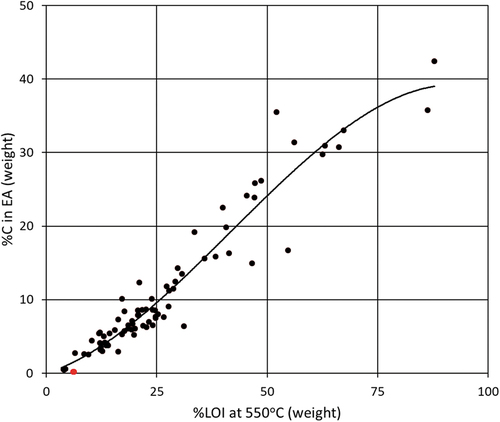
Figure A2. Correlations of (a) SOC 0–30 cm and 0–100 cm storage with plant cover for all profile sites (exponential fits), (b) total SOC storage with full soil depth for all profile sites (second-order polynomial fit), (c) C content with soil moisture for all soil samples (second-order polynomial fit), and (d) C density with soil moisture for all soil samples (second-order polynomial fit). All regressions are significant (p < .05).

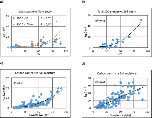
Table A1. Transect and soil profile summary with geographic coordinates, topography (altitude and slope), land cover class, landform type, soil profile depth, surface cover of bare mineral ground including large stones, and total SOC storage.

Transect/profile code	Latitude S	Longitude W	Elevation (m)	Slope (°)	Land cover class	Landform type	Profile depth (cm)	Surface mineral (%)	Total SOC (kg C m^−2)
CG T1-1	43°11.229′	71°14.653′	1,625	10	Alpine dense	Stabilized solifluction	80	20	19.5
CG T1-2	43°11.277′	71°14.719′	1,633	8	Alpine dense	Stabilized solifluction	79	20	20.3
CG T1-3	43°11.331′	71°14.786′	1,650	10	Alpine patchy	Small solifluction lobes	34	90	6.71
CG T1-4	43°11.389′	71°14.865′	1,684	15	Alpine sparse	Small solifluction lobes	25	80	2.04
CG T1-5	43°11.444′	71°14.940′	1,707	5	Alpine sparse	Sorted circles	23	90	2.51
CG T2-1	43°13.591′	71°16.509′	1,910	10	Alpine sparse	Sorted circles	15	90	0.63
CG T2-2	43°13.346′	71°16.538′	1,824	15	Alpine sparse	Small solifluction lobes	43	85	2.46
CG T2-3	43°13.177′	71°16.300′	1,731	1	Alpine dense	Outwash plain	52	25	15.5
CG T2-4	43°12.986′	71°16.050′	1,622	22	Alpine patchy	Solifluction terraces	53	35	7.88
CG T2-5	43°12.888′	71°15.684′	1,521	10	Alpine patchy	Solifluction terraces	66	50	11.2
CG T3-1	43°12.786′	71°16.962′	1,512	7	Dwarf forest	Colluvium	26	0	7.54
CG T3-2	43°12.859′	71°16.926′	1,553	12	Alpine patchy	Colluvium	29	50	2.52
CG T3-3	43°12.930′	71°16.891′	1,604	22	Alpine sparse	Colluvium	18	80	1.08
CG T3-4	43°12.981′	71°16.864′	1,649	22	Alpine sparse	Colluvium/bedrock	37	85	3.50
CG T3-5	43°13.045′	71°16.837′	1,704	30	Alpine sparse	Large stripes	21	92	0.71
VT T1-1	43°58.582′	71°37.010′	1,790	8	Bare	Small stripes	20	100	0.13
VT T1-2	43°58.513′	71°36.827′	1,745	12	Bare	Small stripes	36	100	0.26
VT T1-3	43°58.464′	71°36.659′	1,704	10	Bare	Small stripes	30	100	0.23
VT T1-4	43°58.384′	71°36.386′	1,652	12	Alpine sparse	Colluvium/bedrock	44	95	1.46
VT T1-5	43°58.415′	71°36.214′	1,608	8	Bare	Nivation	28	100	1.43
VT T1-6	43°58.534′	71°36.017′	1,554	10	Alpine dense	Stabilized solifluction	49	0	11.6
VT T2-1	43°58.280′	71°35.416′	1,425	5	Dwarf forest	Colluvium	30	0	3.15
VT T2-2	43°58.289′	71°35.485′	1,435	4	Alpine dense	Outwash plain	44	0	14.8
VT T2-3	43°58.294′	71°35.559′	1,451	10	Alpine patchy	Solifluction terraces	21	8	6.00
VT T2-4	43°58.301′	71°35.632′	1,478	18	Alpine dense	Solifluction terraces	106	0	51.5
VT T2-5	43°58.305′	71°35.710′	1,515	22	Alpine dense	Solifluction terraces	54	<1	14.8
VT T2-6	43°58.310′	71°35.777′	1,552	25	Bare	Nivation	15	100	0.74*

*SOC stock at site VT T2-6 calculated based on soil geochemical properties at site VT T1-5 but considering shallower profile depth.

Table A1.  Continued. Transect and soil profile summary with total plant cover, mean height of upper vegetation stratum, coverage of plant functional types, litter, water and surface mineral bare ground (grain size <4 cm) and large stones (≥4 cm).

Transect/profile code	Plant cover (%)	Height (cm)	Tree (%)	Dwarf shrub (%)	Graminoid (%)	Herb (%)	Cushion (%)	Moss (%)	Lichen (%)	Litter (%)	Water (%)	Bare ground (%)	Large stones (%)
CG T1-1	70	25		3	65	2				10		15	5
CG T1-2	71	25		45	25	1				9		15	5
CG T1-3	10	10			9	1		<1				70	20
CG T1-4	18	25			15	1	1	1		3		60	20
CG T1-5	9	10			7	<1	2	<1				75	15
CG T2-1	9	10		4	5	<1	<1					40	50
CG T2-2	14	10		<1	13	1				1		60	25
CG T2-3	65	10		25	20	<1	20			5	5	10	15
CG T2-4	58	20		40	10	5	3			7		25	10
CG T2-5	45	10		40	5	<1				5		45	5
CG T3-1	75	450	75							100		0	0
CG T3-2	46	15		25	20	1				4		40	10
CG T3-3	18	15		5	11	2	<1			2		70	10
CG T3-4	15	10		10	5							70	15
CG T3-5	8	20		2	6							12	80
VT T1-1	0	0										85	15
VT T1-2	0	0										85	15
VT T1-3	<1	<5				<1				<1		65	35
VT T1-4	4	5		1	3	<1				<1		65	30
VT T1-5	0	0										90	10
VT T1-6	108	15		3	35	40		30			2	0	0
VT T2-1	65	300	65							100		0	0
VT T2-2	95	20		35	55	5				5		0	0
VT T2-3	91	10		82	5	3			1	5		5	3
VT T2-4	99	15		15	59	20		5		1		0	0
VT T2-5	97	20		70	10	15			2	3		<1	<1
VT T2-6	0	0										90	10

References

- Abbott, B. W., J. B. Jones, E. A. G. Schuur, F. S. Chapin III, W. B. Bowden, M. Syndonia Bret-Harte, H. E. Epstein, M. D. Flannigan, T. K. Harms, T. N. Hollingsworth, et al. 2016. Biomass offsets little or none of permafrost carbon release from soils, streams, and wildfire: An expert assessment. Environmental Research Letters 11:34014. doi:10.1088/1748-9326/11/3/034014.
- Aniya, M. 1995. Holocene glacial chronology in Patagonia: Tyndall and Upsala glaciers. Arctic and Alpine Research 27 (4):311–22. doi:10.2307/1552024.
- ArcMap (version 10.3). 2015. Software. Redlands, CA: Esri Inc.
- Bockheim, J. G., and J. S. Munroe. 2014. Organic carbon pools and genesis of alpine soils with permafrost: A review. Arctic, Antarctic, and Alpine Research 46 (4):987–1006. doi:10.1657/1938-4246-46.4.987.
- Bronk Ramsey, C. 2009. Bayesian analysis of radiocarbon dates. Radiocarbon 51 (1):337–60. doi:10.2458/azu_js_rc.51.3494.
- Caldenius, C. C. Z. 1932. Las glaciaciones cuaternarias en la Patagonia y Tierra del Fuego. Geografiska Annaler 14:1–164. doi:10.1080/20014422.1932.11880545.
- Cieraad, E., M. S. McGlone, and B. Huntley. 2014. Southern Hemisphere temperate tree lines are not climatically depressed. Journal of Biogeography 41 (8):1456–66. doi:10.1111/jbi.12308.
- Condom, T., A. Coudrain, J. E. Sicart, and S. Théry. 2007. Computation of the space and time evolution of equilibrium-line altitudes on Andean glaciers (10°N-55°S). Global and Planetary Change 59 (1–4):189–202. doi:10.1016/j.gloplacha.2006.11.021.ird-00270954.
- Copernicus Sentinel Data. 2019. Retrieved from European Space Agency (ESA) November 2018, processed by ESA. Sentinel-2B. 2019. Location, Esquel. Processing center: GCN. 2018-02-15 (T14:28:49). Direction: Descending. WGS84 / UTM zone 18s. Location, Vintter. Processing center: GYS. 2018-02-15. (T14:28:49). Direction: Descending. WGS84 / UTM zone 19s.
- Davies, B. J., C. M. Darvill, H. Lovell, J. M. Bendle, J. A. Dowdeswell, D. Fabel, J.-L. Garcia, A. Geiger, N. F. Glasser, D. M. Gheorghiu, et al. 2020. The evolution of the Patagonian ice sheet from 35 ka to the present day (PATICE). Earth-Science Reviews 204:103152. doi:10.1016/j.earscirev.2020.103152.
- Dean, W. E. 1974. Determination of carbonate and organic matter in calcareous sediments and sedimentary rocks by loss on ignition: Comparison with other methods. Journal of Sedimentary Research 44:242–48. doi:10.1306/74D729D2-2B21-11D7-8648000102C1865D.
- Ding, J., F. Li, G. Yang, L. Chen, B. Zhang, L. Liu, K. Fang, S. Qin, Y. Chen, Y. Peng, et al. 2016. The permafrost carbon inventory on the Tibetan Plateau: A new evaluation using deep sediment cores. Global Change Biology 22 (8):2688–701. doi:10.1111/gcb.13257.
- Espizua, L. E. 2005. Holocene glacier chronology of Valenzuela Valley, Mendoza Andes, Argentina. The Holocene 15 (7):1079–85. doi:10.1191/0959683605hl866rr.
- Earth Explorer. 2000. FS; 083-00; Geological Survey (U.S.).
- Fuchs, M., P. Kuhry, and G. Hugelius. 2015. Low below-ground organic carbon storage in a subarctic alpine permafrost environment. The Cryosphere 9 (2):427–38. doi:10.5194/tc-9-427-2015.
- Google Earth. 2019. Google Earth V 7.3.2. (2010-01-25). Southeast of Esquel, Argentina. 43° 13’ 27“ S, 71° 39’ 17” W, Eye alt 2000-10000 m, (2009-04-13) Northwest of Rio Pico, Lake Vintter, Argentina. 43° 59’ 33“ S, 71° 38’ 46” W, Eye alt 2000-10000 m. DigitalGlobe. 2019. Landsat / Copernicus NASA image 2019. http://www.earth.google.com [2019-01-01].
- Gorbunov, A. P. 1978. Permafrost investigation in high mountain regions. Arctic and Alpine Research 10 (2):283–94. doi:10.1080/00040851.1978.12003967.
- Guijarro, J. A. 2019. Climatol: Climate tools (series homogenization and derived products). https://cran.r-project.org/web/packages/climatol/.
- Haeberli, W. 1985. Creep of mountain permafrost: Internal structure and flow of alpine rock glaciers. Mitteilungen der Versuchsanstalt für Wasserbau, Hydrologie und Glaziologie, ETH Zürich 77, Zurich: ETH.
- Haeberli, W., C. Guodong, A. Gorbunov, and S. Harris. 1993. Mountain permafrost and climatic change. Permafrost and Periglacial Processes 4 (2):165–74. doi:10.1002/ppp.3430040208.
- Haller, M. J., R. R. Lech, O. Martínez, C. M. Meister, S. Poma, and Y. R. Viera. 2010. Hoja Geológica 4372-III/IV, Trevelin, provincia del Chubut. Instituto de Geología y Recursos Minerales, Servicio Geológico Minero Argentino, Boletín 322, 86p., Buenos Aires.
- Hammer, Ø., D. A. T. Harper, and P. D. Ryan. 2001. PAST: Paleontological statistics software package for education and data analysis. Palaeontologia Electronica 4:9.
- Hastenrath, S. 1971. Beobachtungen zur k1ima-morphologischen Hohenstufung der Cordillera Real (Bolivien). Erdkunde 25 (2):102–08. doi:10.3112/erdkunde.1971.02.03.
- Heiri, O., A. F. Lotter, and G. Lemcke. 2001. Loss on ignition as a method for estimating organic and carbonate content in sediments: Reproducibility comparability of results. Journal of Paleolimnology 25 (1):101–10. doi:10.1023/A:1008119611481.
- Hogg, A., T. Heaton, Q. Hua, J. Palmer, C. Turney, J. Southon, A. Bayliss, P. Blackwell, G. Boswijk, C. Bronk Ramsey, et al. 2020. SHCal20 Southern Hemisphere calibration, 0–55,000 years cal BP. Radiocarbon 62 (4):759–78. doi:10.1017/RDC.2020.59.
- Huete, A. R. 1988. A soil-adjusted vegetation index (SAVI). Remote Sensing of Environment 25 (3):295–309. doi:10.1016/0034-4257(88)90106-X.
- Hugelius, G. 2012. Spatial upscaling using thematic maps: An analysis of uncertainties in permafrost soil carbon estimates. Global Biogeochemical Cycles 26 (2):GB2026. doi:10.1029/2011GB004154.
- Hugelius, G., J. Strauss, S. Zubrzycki, J. W. Harden, E. A. G. Schuur, C.-L. Ping, L. Schirrmeister, G. Grosse, G. J. Michaelson, C. D. Koven, et al. 2014. Estimated stocks of circumpolar permafrost carbon with quantified uncertainty ranges and identified data gaps. Biogeosciences 11 (23):6573–93. doi:10.5194/bg-11-6573-2014.
- Japan Aerospace Exploration Agency. 2021. ALOS World 3D 30 meter DEM. V3.2, Jan 2021. ALOS World 3D 30 meter DEM. 10.5069/G94M92HB. Accessed: 2021-02-08
- Jones, H. G., and R. A. Vaughan. 2010. Remote sensing of vegetation: Principles, techniques, and applications, 365. New York: Oxford University Press.
- Kuhry, P., E. Dorrepaal, G. Hugelius, E. A. G. Schuur, and C. Tarnocai. 2010. Potential remobilization of belowground permafrost carbon under future global warming. Permafrost and Periglacial Processes 21 (2):208–14. doi:10.1002/ppp.684.
- Kuhry, P., E. Makopoulou, D. Pascual, I. Pecker Marcosig, and D. Trombotto Liaudat. in press. Soil organic carbon stocks in the high mountain permafrost zone of the semi-arid Central Andes (Cordillera Frontal, Argentina). Catena.
- Leger, T. P. M., A. S. Hein, R. G. Bingham, M. A. Martini, R. L. Soteres, E. A. Sagredo, and O. A. Martínez. 2020. The glacial geomorphology of the Río Corcovado, Río Huemul and Lago Palena/General Vintter valleys, northeastern Patagonia (43°S, 71°W). Journal of Maps 16 (2):651–68. doi:10.1080/17445647.2020.1794990.
- Magrin, G. O., J. A. Marengo, J.-P. Boulanger, M. S. Buckeridge, E. Castellanos, G. Poveda, F. R. Scarano, and S. Vicuña. 2014. Central and South America. In Climate change 2014: Impacts, adaptation, and vulnerability. Part B: Regional aspects. Contribution of working group II to the fifth assessment report of the intergovernmental panel on climate change, ed. V. R. Barros, C. B. Field, D. J. Dokken, M. D. Mastrandrea, K. J. Mach, T. E. Bilir, M. Chatterjee, K. L. Ebi, Y. O. Estrada, R. C. Genova, et al., 1499–566. Cambridge, United Kingdom and New York, NY, USA: Cambridge University Press.
- Palsar, A.L.O.S. 2011. DEM-Data 12.5 m resolution. Advanced Land Observing Satellite-1 (ALOS), Phased Array type L-band Synthetic Aperture Radar (PALSAR). Source NASA DEM Product 2011.
- Pascual, D., P. Kuhry, and T. Raudina. 2020. Soil organic carbon storage in a mountain permafrost area of Central Asia (High Altai, Russia). Ambio. doi:10.1007/s13280-020-01433-6.
- Peel, M. C., B. L. Finlayson, and T. A. McMahon. 2007. Updated world map of the Köppen-Geiger climate classification. Hydrology and Earth System Sciences 11 (5):1633–44. doi:10.5194/hess-11-1633-2007.
- Pereyra, F. X., and P. Bouza. 2019. Soils from the Patagonian region. In The soils of Argentina. World soils book series, G. Rubio, R. Lavado, and F. Pereyra. ed., Cham: Springer. doi:10.1007/978-3-319-76853-3-7.
- Reato, A., O. A. Martinez, D. Serrat, and D. M. Cano. 2017. Glaciarismo y periglaciarismo cuaternario en el Cerro Nahuel Pan, sector extra-andino del Chubut, Argentina. In XX Congreso Geologico Argentino. San Miguel de Tucuman, 78–83.
- Ruiz, L., and D. Trombotto Liaudat. 2012. Mountain permafrost distribution in the Andes of Chubut (Argentina) based on a statistical model. Proceedings of the Tenth International Conference on Permafrost (TICOP), Salekhard, Russia, pp. 365–70.
- Saito, K., D. Trombotto Liaudat, K. Yoshikawa, J. Mori, T. Sone, S. Marchenko, V. Romanovsky, J. Walsh, A. Hendricks, and E. Bottegal. 2015. Late quaternary permafrost distributions downscaled for South America: Examinations of GCM-based maps with observations. Permafrost and Periglacial Processes 27 (1):43–55. doi:10.1002/ppp.1863.
- Schuur, E. A. G., A. D. McGuire, C. Schädel, G. Grosse, J. W. Harden, D. J. Hayes, G. Hugelius, C. D. Koven, P. Kuhry, D. M. Lawrence, et al. 2015. Climate change and the permafrost carbon feedback. Nature 20 (7546):171–79. doi:10.1038/nature14338.
- Soil Survey Staff. 2014. Keys to soil taxonomy, 12th Edition. United States Department of Agriculture-Natural Resources Conservation Service, Washington.
- Tarnocai, D. C., C. J. G. Canadell, E. A. G. Schuur, P. Kuhry, G. Mazhitova, and S. Zimov. 2009. Soil organic carbon pools in the northern circumpolar permafrost region. Global Biogeochemical Cycles 23 (2):GB2023. doi:10.1029/2008GB003327.
- Thompson, S. K. 1992. Sampling, 343. New York: John Wiley.
- Trombotto, D. 2000. Survey of cryogenic processes, periglacial forms and permafrost conditions in South America. Revista Do Instituto Geológico Sao Paulo 21 (1–2):33–55. doi:10.5935/0100-929X.20000004.
- Trouet, V., and G. J. Van Oldenborgh. 2013. KNMI Climate Explorer: A Web-Based Research Tool for High-Resolution Paleoclimatology. Tree-Ring Research 69:3–13. doi:10.3959/1536-1098-69.1.3.
- Turetsky, M. R., B. W. Abbott, M. C. Jones, K. Walter Anthony, D. Olefeldt, E. A. G. Schuur, G. Grosse, P. Kuhry, G. Hugelius, C. Koven, et al. 2020. Carbon release through abrupt permafrost thaw. Nature Geoscience 13 (2):138–43. doi:10.1038/s41561-019-0526-0.
- Walter, H., and H. Lieth. 1967. Klimadiagramm-Weltatlas. Jena: Gustav Fischer Verlag.
- Wojcik, R., J. Palmtag, G. Hugelius, N. Weiss, and P. Kuhry. 2019. Land cover and landform-based upscaling of soil organic carbon stocks on the Brøgger Peninsula, Svalbard. Arctic, Antarctic, and Alpine Research 51 (1):40–57. doi:10.1080/15230430.2019.1570784.
- Zimmermann, M., P. Meir, M. R. R. Silman, A. Fedders, A. Gibbon, Y. Malhi, D. H. Urrego, M. B. Bush, K. J. Feeley, K. C. Garcia, et al. 2010. No differences in soil carbon stocks across the tree line in the Peruvian Andes. Ecosystems 13 (1):62–74. doi:10.1007/s10021-009-9300-2.