Timing of glacial - non-glacial stages in Finland: An exploratory analysis of the OSL data

ABSTRACT

The Optically Stimulated Luminescence (OSL) age database of Finland was established, and it includes all of the published OSL age results from different sediment sequences in Finland. The OSL database includes ~180 published OSL ages ranging from 235,000 years to 300 years; that is, from the Middle Saalian interstadial to the present. Two statistical clustering methods, K-means and model-based clustering with the package mclust, were used to analyze the internal structure of the assembled OSL data. The results of these analyses were also compared to the established Northwest European (Fennoscandian) chronostratigraphical stages. When the data were analyzed by the K-means method, the “right” number of clusters (K) was seven. The model-based clustering method (K = five) created bigger clusters for the youngest and the oldest ages compared to the K-means clusters. Both methods show that the ages followed the increasing trend from the youngest to the oldest, and the standard error of ages was constantly increasing except in the age group 70–115 ka, where the standard errors were exceptionally high. Seven clusters obtained from the age data corresponded relatively well with the number of stratigraphically established interglacials and interstadials in the late Middle and Late Pleistocene in Fennoscandia. The exceptionally large standard error of ages in the Early Weichselian age group 70–115 ka might result from mixing of heterogeneous and poorly or partly bleached mineral material from both Eemian and Early Weichselian sediment layers. The OSL-dated Middle Saalian interstadial sediments in the data support a strong stadial and interstadial variation also before the Late Pleistocene.

KEYWORDS:

• Optically Stimulated Luminescence
• database
• interglacial
• interstadial
• clustering
• statistical analysis

Introduction

The number and duration of Weichselian (between 115,000 and 11,700 years) stadials and interstadials in Fennoscandia and elsewhere in formerly glaciated areas have been widely discussed in recent decades (Svendsen et al. 2004; Auri et al. 2008; Johansson, Lunkka, and Sarala 2011; Helmens 2014a; Räsänen et al. 2015; Dalton et al. 2016). An old hypothesis of a single glaciation covering vast areas of Europe and North America during almost the whole of the Weichselian Stage has evolved into a multiphase glaciation hypothesis (e.g., Hirvas 1991; Lundqvist 1992; Nenonen 1995; Helmens and Engels 2010), which includes the idea that vast Northern Hemisphere ice sheets waxed and waned several times during the last glaciation. These ice sheet fluctuations can broadly be correlated with climatic proxy data from ice cores and marine sediments (e.g., Helmens 2014b). Based on recent studies, it seems that glaciation centers—for example, in Fennoscandia—were deglaciated and ice-free several times, not only during the Weichselian Stage but also during the Saalian Stage (e.g., Johansson, Lunkka, and Sarala 2011; Putkinen et al. 2020).

Estimation of the time and length of stadial–interstadial variations and the ice extent in formerly glaciated terrestrial areas such as Fennoscandia is largely based on the correlation of litho- and biostratigraphical results from glacigenic and nonglacigenic sediment sequences to the well-established marine isotope stages (MIS) and/or Greenland ice core chronologies (e.g., Greenland interstadial record; cf. Batchelor et al. 2019). However, terrestrial glacigenic sequences are in most cases incomplete sediment successions full of erosional gaps and void of organic sediments and therefore are not suitable for wider stratigraphical correlation purposes. Therefore, Optically Stimulated Luminescence (OSL) dating of sand- and silt-rich sediments in multiple till sequences has brought valuable and spatially dense enough records from the terrestrial, inter-till sediment layers to estimate palaeoclimate variations during the latest glaciations.

Finland, located in the center of the Fennoscandian Ice Sheet (FIS), was covered by ice several times during the Quaternary. Repeatedly occurring cold-based subglacial conditions and the location of the ice-divide zone over northern Finland during deglaciation phases has enabled the preservation of old glacigenic and interglacial/-stadial deposits, particularly in northern but also in central-western Finland (Johansson, Lunkka, and Sarala 2011). Thus, the Finnish till stratigraphy consists of several superimposed till beds. The most complete one with six stratigraphically significant till beds has been described from northern Finland (Hirvas 1991). Observations of tens of inter-till stratified silt, sand, and/or gravel deposits have been recorded, and many of the inter-till stratified clastic sediments also include organic peat and/or gyttja. Most of the organic sediments in these sediment sequences have yielded radiocarbon ages over 40 ka (Hirvas 1991; Nenonen 1995). These radiocarbon ages are considered unreliable due to the radiocarbon dating range, conventionally only eight half-lives; that is, c. 40 ka (e.g., Hirvas 1991).

There are two possible options to study ancient climate changes with respect to changing glacial and ice-free conditions in the central areas of formerly glaciated terrains. First, there is a till stratigraphical approach where the lateral extent of each separate till unit is estimated using mainly till clast fabric data and other diagnostic characteristics of each till bed. This type of approach is the only viable option when a sediment section contains only till units but no organic and/or sorted sediment beds. Till stratigraphy can be placed into a wider stratigraphical context when inter-till stratified and/or organic beds occur in sediment sequences. At these sites, biostratigraphical methods (for example, pollen and macrofossil analyses) can be used to establish a firm stratigraphy for the site and place the till units occurring in a wider area into the stratigraphical order. Thus, different till units indicate cold, glacial conditions, when glaciers have covered terrains and eroded sediments that subsequently will be redeposited as till in different moraine formations. Under suitable, preserving conditions, each till unit represents a separate glacial phase and can be used in tracing back the glacial history of an area (e.g., Hirvas 1991). Unlike till units, inter-till stratified sediments with organic material reflect warm, ice-free conditions that prevailed between the glacial phases. The other option to study climate history and particularly variations of cold, glacial conditions and warm, ice-free interglacial/interstadial conditions of formerly glaciated terrains is to date inter-till stratified sediments directly with the radiocarbon and/or OSL dating methods. Deposition of stratified clastic sediments, mainly gravel, sand, and silt/clay, is the highest when glaciers are melting and produce glaciofluvial deposits, which are also the source material for eolian and lacustrine/marine sediments laid down during interstadials and interglacials. The influence of sunlight to the bleaching of electron traps in mineral grains during sediment transportation prior to deposition is crucial and can be effective on deglacial stratified sediments and subsequently formed interglacial/-stadial clastic sand and silt sediments. If transportation history of sediments and their depositional environment can be defined and it is ascertained that sediment grains have been exposed to light during their transportation, the OSL method can be used to date deglacial and interglacial and stadial sand and silt/clay-rich sediments. However, it is highly important to use both stratigraphic and geochronological approaches to unravel the glacial/interglacial history in formerly glaciated areas.

The OSL method has been used as a dating method in Finland since the beginning of 1990s (e.g., Hutt et al. 1993; Nenonen 1995). This method has provided an opportunity to date the Saalian and Late Pleistocene inter-till stratified sediment deposits found from different stratigraphically controlled sites in Finland. Many of the inter-till layers have been OSL-dated back to the Eemian or Early Weichselian (e.g., Mäkinen 2005; Sarala et al. 2005; Sarala and Rossi 2006; Helmens et al. 2007; Alexanderson, Eskola, and Helmens 2008; Auri et al. 2008; Pitkäranta 2008, 2009; Salonen et al. 2008; Sarala 2011; Sarala and Patisson 2011; Pitkäranta, Lunkka, and Eskola 2013; Howett et al. 2015; Lunkka, Sarala, and Gibbard 2015; Lunkka et al. 2016; Åberg et al. 2020) or even to the Middle Saalian (Auri et al. 2008; Lunkka, Sarala, and Gibbard 2015; Putkinen et al. 2020), and OSL and ¹⁴C ages falling into the Middle Weichselian and last deglaciation are also common (Käyhkö et al. 1999; Kotilainen 2004; Sarala and Rossi 2006; Lunkka, Murray, and Korpela 2008; Sarala et al. 2010, 2016; Hyttinen, Kotilainen, and Salonen 2011; Johansson, Lunkka, and Sarala 2011; Sarala and Eskola 2011; Matthews and Seppälä 2013; Salonen et al. 2014). These published ages form an extremely valuable resource and are here compiled into the first easily accessible Finnish OSL age database (Supplementary data).

In recent years, the popularity of cluster analysis has increased in many research fields. The objective of clustering is to assign unlabeled data points into groups called clusters based on their similarity. Clustering is especially advantageous in cases where the size of the data sets is large and no prior information of the structure is available (e.g., Darkins et al. 2013; Aghabozorgi, Shirkhorshidi, and Wah 2015). Though significant for reasons discussed above, on their own, the individual Finnish OSL age data sets are too small for conclusive analysis of the structure. Compiling them increases the size of the data set and enables the distinction of features within it. Available as a whole for the first time, the Finnish OSL age database offers an excellent opportunity for exploratory analysis. In this work, two different approaches were used in the R environment, distance-based algorithm K-means and model-based algorithm mclust, to characterize the distribution and standard error of the OSL age data of the Finnish OSL age database. Also tested is whether the use of the cluster analysis methods to characterize abundant OSL data will shed light on timing of different glacial and ice-free interglacial and interstadial events in Finland.

Regional setting

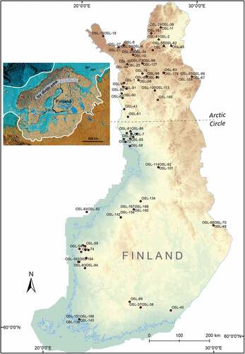
Finland is located in Northeastern Europe (Figure 1). Its bedrock forms a part of the Archean and Proterozoic Fennoscandian Shield, composed of crystalline rocks (mainly granitoids and gneisses). The area has been overrun by glacial ice several times during the Quaternary due to its location in the center of the former Fennoscandian Ice Sheet realm (Donner 1995; Johansson, Lunkka, and Sarala 2011). Particularly in northern Finland, cold-based glacial conditions and permafrost prevailed for a long time during glaciations. These conditions led to the formation of stagnant, subglacial environment with a limited amount of erosion. This resulted in the widespread preservation of preglacial weathered bedrock regolith, landforms such as tors, and a thick glacigenic overburden composed of multiple till sequences and inter-till stratified sediments (Hirvas 1991; Hall, Sarala, and Ebert 2015).

Figure 1. Location of the OSL data observation points based on published data before 2020 in Finland (see Supplementary data), in the central part of Last Glacial Maximum. Modified from Sarajärvi (2020).

Based on published literature, it can be concluded that the glacial history of Finland dates back several hundred thousand years (Johansson, Lunkka, and Sarala 2011). Hirvas (1991) made an estimation that the oldest till layer in Finnish Lapland was deposited during the Elsterian glaciation (475,000–370,000 years ago). This estimation was based on till stratigraphy where litho- and biostratigraphy (mainly pollen stratigraphy) from multiple till sequences and the inter-till, organic-bearing stratified layers were applied to reconstruct the glaciation history for Finnish Lapland. In the 1970s and 1980s there were no applicable absolute dating methods to date sediments older than c. 40,000 years old (i.e., the upper limit of radiocarbon dating method) and, therefore, stratigraphical correlation of sediments older than the late Middle Weichselian was mainly based on biostratigraphical argumentation.

Some of the sediment units that, for example, Hirvas (1991) correlated to the pre-Eemian (older than MIS 5e) ice-free interstadials/glacials have subsequently been OSL dated to the Eemian or younger than the Eemian interglacial (Sarala 2011; Lunkka, Sarala, and Gibbard 2015). However, several sedimentological studies in recent decades that include OSL age determinations on interstadial and interglacial sediments have confirmed that till units and sorted sediments of the Saalian age occur particularly in northern and western Finland (e.g., Sarala 2005b; Johansson, Lunkka, and Sarala 2011; Putkinen et al. 2020). There is a lot of evidence and many studies on the occurrence of stadial and interstadial/-glacial deposits in Finland, and in this article, the age data are introduced and discussed.

Materials and methods

OSL age database

At present, there are more than 200 OSL dating samples collected from Finland, of which about 180 were published between 1993 and 2020 (Supplementary data). For the Finnish OSL age database, the data were collected from published articles that were found during a literature review (Sarajärvi 2020). The collected data include the sample metadata and descriptions of sampled materials together with water contents, paleodoses (equivalent dose), dose rates, and calculated ages and their standard errors if available in the original data. Unfortunately, many publications do not present metadata, and some data are missing (e.g., water content, paleodoses, and number of countings, as well as the methodological descriptions of sample and data processing and statistical analyses of the results). Most of the age determinations were done in the Laboratory of Chronology/Dating Laboratory of the University of Helsinki, and the Nordic Laboratory for Luminescence Dating (Aarhus University) at Risø DTU, Denmark, based on single aliquot regeneration protocol (Murray and Wintle 2000).

The OSL ages compiled in the data set span a range from c. 300 years to 235,000 years before present. Although the data set includes many dating results, their spatial coverage is not extensive. The sampling sites are centered in the northern and the western coastal areas of Finland (Figure 1), whereas large areas where the Quaternary deposits occur are still poorly studied and lack suitable sediments for dating. This phenomenon reflects glacial stratigraphy in Finland and indicates the presence of thick stratigraphic sections close to the latest cold-based, inner parts of the FIS, whereas the eastern and southern parts are missing the observations of inter-till stratified sediment layers. Due to the high number of source articles for the database and very heterogenic descriptions of the stratigraphy and sample materials, our focus is more on classification of data instead of deeper sedimentological analyses.

Classification of the dated sediments in the database

Based on the reported observations of the OSL dated sediment layers (Supplementary data), most samples were collected from the inter-till sandy and/or silty layers or from fine sand of the postglacial eolian deposits (the youngest ages). They were described to represent glaciofluvial/-lacustrine or in some cases fluvial/lacustrine sediments (including cross-stratification, ripple marks, graded bedding). Although bleaching of sediments during sediment transport is highly variable and depends on depositional environment, the dated sediment types in the database can be divided into two classes: Class 1 is glaciolacustrine/lacustrine deltaic fine sand/silt (littoral and sublittoral sand and silt) and Class 2 is glaciofluvial/-lacustrine or fluvial/lacustrine stratified sand (deltas, sub- and supra-aquatic fans, nonglaciofluvial rivers).

In this database, the published OSL age determinations made from glaciofluvial medium/coarser sand sediments form Class 3 in the data. This sediment type represents sediments deposited under fast water flow conditions at the ice margin (subglacial tunnel mouth) and at the proximal part of glaciofluvial deltaic/subaquatic fan or sandur environments.

Class 4 in the data set consists of gravels and sands that have been collected from sediment beds representing lacustrine or glaciolacustrine littoral deposits.

There are also quite a few OSL age determinations from ice-wedge cast sand infills and eolian dune sediments (Class 5). Most of the OSL ages come from eolian sediments deposited during the last deglaciation and the Holocene.

Cluster analysis

The aim of cluster analysis is to find the dependencies between the characteristics (unifying and distinguishing factors) of the data by grouping similar observations and/or variables into clusters. In this study, the observational data (see Supplementary data) were grouped using the aforementioned factors of age, standard error of age, dose rate, and paleodose. To maximize the number of usable observation values, sediment type and water content were not used as factors in the clustering because they were not available for all observations.

K-means method

K-means is a model-free clustering algorithm available in many statistical programming software packages. With model-free approaches, no prior assumptions on the distribution of the data are made. Instead, the process is based on dissimilarity measures; for example, the distance between the data points. With K-means, each of the data points can be assigned to only one cluster (hard clustering) so that the variance within each cluster is minimized. It is commonly advisable to run the algorithm several times because the local optimum solution may not be the global optimum solution (James et al. 2014). One of the notable shortcomings of the K-means clustering is determining the right number of clusters, K. Here, the “right” number of clusters refers to a solution—that is, a fit to the data—where any additional components do not add to the descriptive power (the point of diminishing results). When no objective true value is known, the best guess can be obtained using gap statistics or the elbow method (for example, between-cluster sum of squares [BSS]/total sum of squares [TSS]) or information criteria such as the Bayesian information criterion or Akaike information criterion. Though the solutions obtained with these methods are not definitely true, the right number of clusters is, in general, highly subjective (see, e.g., Kaufman and Rousseeuw 1990).

In this work, R implementation of K-means algorithm, the function kmeans(), was used (see RDocumentation 2021). A basic rundown of the K-means algorithm is given here. The technical details can be found in, for example, James et al. (2014) and Hartigan and Wong (1979). The algorithm is initialized by giving it the number K; that is, the number of clusters the data to be fitted. By default, each of the data points is randomly assigned a number 1,2, …, K and the centroids of these random partitions are calculated. The nearest neighbors of these centroids are then chosen to form clusters C₁, …, C_K for which new centroids are calculated. The sums of squared distances from the new centroids are then calculated within these clusters. A data point is assigned to another cluster if this decreases the value of the sum. The process described is then iterated until no data points change the clusters or the algorithm reaches the default or a set number of iterations. The function then returns an object containing the outcome of the process and other useful information about the clusters.

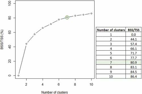
Before the clustering, samples with missing values in the variables used in the clustering were excluded from the data set. Additionally, the data were scaled¹ because the difference in the range of values between the variables was considerable. To ensure that the clustering process went to completion, the value of parameter iter.max = 50 was set for all runs. Even though there was little variation in the solutions between the runs, the best solution of five runs was selected for each value of K. The elbow method was then used to help determine the right number of clusters (Miquez 2007). By trying many values of K, the resulting ratios of BSS and TSS were plotted with higher values of the ratio, BSS/TSS, indicating a better fit to the data. A point of diminishing returns, or the “elbow,” was then chosen according to a plot shown in Figure 2, aided by a visual inspection of the found clusters. The optimum solution for the number of clusters, K = 7, was selected.

Figure 2. A plot of between-cluster sum of squares divided by the total sum of squares (BSS/TSS ratios) for different values of K. The “elbow” is marked by the green circle. The “right” number of clusters as indicated by the plot is six to eight.

Model-based clustering method

Model-based clustering can be used to obtain a cluster partition; that is, an assignment of each observation to one specific cluster. The resulting assignment, however, is not just a “hard” assignment, but it provides results in a probability of an observation belonging to each cluster. As the name indicates, model-based clustering makes use of a statistical model for the shape of the clusters. The standard model is a multivariate normal distribution; that is, it is assumed that every cluster originates from a density of a multivariate normal distribution, with a certain location and covariance. This is an advantage over K-means clustering because the cluster shapes can be more flexible. The result of K-means is typically spherically shaped clusters (due to the use of Euclidean distances to the center).

A detailed description of model-based clustering can be found in Fraley and Raftery (2002) and many other sources by these authors. It is assumed that the data consist of K clusters, generated by multivariate normal densities with expectation µ_k and covariance Ʃ_k, for k = 1, …, K. Further, the class probabilities are given by so-called mixing coefficients π₁, …, π_K, where π₁ + … + π_K = 1.

All of these parameters are unknown, and they are estimated using the expectation-maximization algorithm. Note that if the underlying data consist of p variables, the involved covariance matrices are p × p matrices, and for larger p there are many parameters to estimate from the available data, which can lead to instability. For this reason, the cluster “models” can be simplified by imposing restrictions on the cluster covariance structures. The simplest possibility for such restrictions is that all covariance matrices have a diagonal form, with variance σ² in the diagonal. This would imply that all clusters are spherical with the same radius in all directions. Thus, the estimation of the covariances reduces to estimate only one parameter, the variance σ². A less restricted covariance structure is that Ʃ_k is again of diagonal form, with diagonal elements ${\sigma }_k^2$, for k = 1, …, K. In this case, the clusters are still spherical, but their size can be different according to their variance ${\sigma }_k^2$, which needs to be estimated. There are many more possibilities of imposing different restrictions on the covariance structure; for details, we refer to Fraley and Raftery (2002). Because the parameter estimation is done in a maximum likelihood framework, one can compute a criterion such as the Bayesian information criterion to select the most appropriate cluster model (Schwarz 1978). Furthermore, one can use the same criterion to select the most appropriate number of mixture components and thus the most useful number K of clusters. The R package mclust (Fraley et al. 2012) implements a model-based clustering. The function mclust() can also take an argument to compute all cluster solutions for a varying number of clusters.

Results

K-means methods results

Figure 3 presents a scatterplot matrix of the seven-cluster solution from K-means clustering using function kmeans(). A scatterplot matrix presents each variable against another one. For example, the plot in row 1 and column 2 shows variable “Standard error_ka” (horizontal) against variable “Age_ka” (vertical), and for the plot in row 2 and columns 1 these axes are reversed. The numbers in the plots refer to the scale of these variables. The different colors correspond to the different identified clusters. Here, the cluster number or color is not important, but the most important point is the assignment of the observations into different clusters. It can be seen from the plot (Figure 3) that the standard error in age changes a lot with the age of the samples. This has also been captured in the clustering when looking at the purple circles in the Age_ka − Standard error_ka plot (Figure 3). Though there is an overlap in the clusters, with respect to standard error, paleodose, and dose rate, one can see distinct spherical clusters that are typical for K-means.

Figure 3. The K-means algorithm applied to the OSL data results in an optimal number of clusters of seven. This seven-cluster solution is shown in the scatterplot matrix, where all variable pairs (age [ka], age standard error [ka], dose rate [Gy/ka], and paleodose [Gy]) are shown against each other, in their original units. The colors for the observations are according to the cluster assignments to the seven clusters.

Most of the Holocene age OSL results have been obtained from the eolian sediments in northern Finland. Cluster 1 represents this data set, where the OSL ages range between 0 and 46 ka, with a mean age of 13.5 ka and a mean standard error of c. 1.8 ka (Figure 3 and Table 1). The Late Weichselian and the late Middle Weichselian ages belong to cluster 4, where the mean age is c. 15.9 ka. The main reason that separates cluster 4 from cluster 1 is the high dose rate. The main portion of the earlier part of the Middle Weichselian ages is included in cluster 7, where the mean age is c. 57.9 ka. However, this cluster also includes some portion of the Early Weichselian ages and particularly those that have a low variation (mean standard error value 5.6). For clusters 1, 4, and 7 it is typical that the variation in the determined ages is relatively low.

Table 1. Basic parameters of the seven clusters formed after using function kmeans().

Cluster	1	2	3	4	5	6	7
Age min.	0.2	46.8	120.0	0.4	87.0	58.1	22.0
Age mean	8.9	80.4	165.5	15.9	120.6	85.6	57.9
Age max.	46.0	123.0	235.0	39.0	163.0	133.0	115.0
Standard error min.	0.1	5.0	10.0	0.1	9.0	11.6	2.0
Standard error mean	1.8	10.3	14.8	1.9	13.4	18.8	5.6
Standard error max.	6.1	16.0	19.0	5.0	19.0	28.0	11.3

The ages dated back to the Early Weichselian time are included in clusters 2 and 6, in which main ages are 81.2 and 85.6 ka. In those clusters, the standard error of the ages is high (10.3 and 18.8 ka). Particularly in cluster 6, the standard errors are the highest of all clusters.

Clusters 3 and 5 represent the oldest age groups in the data. Cluster 5 includes most of the Eemian ages having the mean age of c. 120 ka. There are also some ages from the early part of the Early Weichselian as well as some ages from the latest phase of the Saalian Stage. Cluster 3 includes the oldest age groups, which dated back to the Late and Middle Saalian Stages (mean age about 173 ka; oldest ages 235 ka).

Model-based clustering results

Figure 4 presents the solution from model-based clustering in a scatterplot matrix, where each variable is shown against every other variant. When applying the mclust() function over the age data, the optimal model gave the result K = 5 clusters, with individual covariance structures. The plots show the estimated cluster centers and shapes (ellipses), and the observations are presented with different colors and different symbols as they are assigned to the five clusters (cluster 1 representing the youngest age group and cluster 5 the oldest). Particularly in Dose_rate plots, the clusters are relatively well separated, whereas in Age_ka plots and Standard error_ka plots, the clusters follow the increasing trend of these variables.

Figure 4. The model-based cluster algorithm using the function mclust() results in an optimal model with K = 5 clusters and visualizes the estimated cluster centers and shapes (ellipses). This five-cluster solution is shown in the scatterplot matrix with the scales in the original units (age [ka], age standard error [ka], dose rate [Gy/ka], and paleodose [Gy]) and with different colors of the observations as they are assigned to the clusters; the ellipses indicate the cluster shapes.

An advantage of this clustering procedure is that once the parameters have been estimated, the models can be used to assign new observations to one of the clusters.

Discussion

Influence of sediment variation

The Finnish OSL age database includes about 180 OSL age determinations. The OSL samples dated are mostly from sand and/or silt inter-till layers or fine sand from the postglacial eolian deposits and grouped into five sediment classes as described above.

In glaciated terrains, glaciofluvial and -lacustrine sediments (sands and silts) are the most common stratified sediment types and also dominant sample material for the OSL dating in the Finnish OSL age database. Deposition of these type of sediments occurs further away from the ice margin in both sub- and supra-aquatic environments. If glaciofluvial sands and gravels are released from beneath the ice margin into a glaciolacustrine or proximal glaciofluvial environments next to the ice margin (here sediment Classes 2 and 3), sediments normally have a short transport distance. In addition, the deposition rate is typically very high and light-shielding effects due to high suspended load, ice-block shadows, and deposition at night might cause incomplete bleaching not only in coarse gravel and sand sediments but also in fine sand suspended material (e.g., Rhodes 2011; Lunkka, Palmu, and Seppänen 2021). Furthermore, erosion and redeposition can disturb the settling of the sandy material and cause mixed sediment layers with well- and poorly bleached grain populations. However, in braided river systems, such as sandur and braid plains; in the distal delta topset environments; and in littoral zones of glaciolacustrine and lacustrine basins (here sediment Classes 1 and 4), the bleaching potential of mineral grains increases and the OSL samples obtained especially from sands in the littoral zones of glaciofluvial formations yield reliable ages (e.g., Fuchs and Owen 2008). This topic has been discussed by, for example Houmark-Nielsen (2008), Thrasher et al. (2009), Alexanderson and Murray (2012), and King, Robinson, and Finch (2014).

In the OSL age database, sand in ice-wedge casts (Class 5) indicates the presence of patterned ground in a periglacial environment and the sand filling the cracks of the patterned ground ice wedges is the most suitable material for high-quality OSL dates. Similarly, eolian sands (Class 5), originally derived from glaciofluvial and -deltaic sands, occurring in supra-aquatic fossilized dune areas are well bleached and suitable for OSL dating. Although most of the eolian sands in Finland are sand dunes related to the last deglaciation or represent beach dunes formed during a general water level regression of the Baltic basin (e.g., Koutaniemi 1979; Kotilainen 2004), in some sites eolian sands can be found beneath till units representing remnants of ancient sand dunes deposited well before the last deglaciation.

Commonly, a sampled sediment unit and its depositional environment and stratigraphic position were not comprehensively described in the articles from which the OSL age database was compiled. This was especially the case if the samples were obtained from boreholes or from small natural sediment exposures with poor stratigraphic control. This undoubtedly affects the quality of the OSL ages. Therefore, quality control of the OSL age database in the future should include more precise sedimentological and stratigraphic attributes that enable assessment of the quality of OSL ages. In the present OSL age database only broad environmental and stratigraphical attributes (Classes 1–5) were possible to derive from the published articles, but even these broad environmental categories revealed clear clusters in the OSL age data.

Interpretation of the clustering results

The K-means cluster analysis revealed that the age groups formed from the Finnish OSL age data structure have a good correlation with known interglacial/interstadial stage age distribution during the Saalian and Late Pleistocene. The Eemian and the Early Weichselian ice-free phases in Finland are well known, and a large portion of the ages are grouped into clusters 2, 5, and 6. Furthermore, the ages in clusters 1 and 4 represent known ice-free conditions during the Holocene and the last deglaciation. However, clusters 1 and 4 also include some Middle Weichselian ages. The reason for this seems to be a strong influence of the dose rates to the clustering seen both in the K-means and mclust clustering (see Figures 3 and 4). Cluster 3 also includes a group of ages representing the Middle Saalian interstadials.

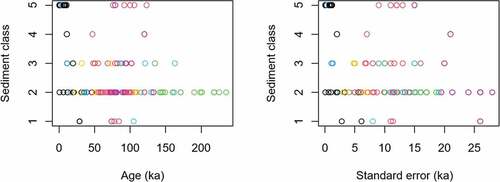
The model-based clustering using the function mclust() gave five clusters for the OSL age data. The main difference compared to the K-means clustering method is the grouping of the oldest ages together and dividing the Middle Weichselian ages into the Early Weichselian clusters and the Late Weichselian cluster. However, this approach also highlights the high standard error of ages in the second portion of Early Weichselian ages. There could be several reasons for the high standard errors, such as mixture of sediments of different ages, resedimentation, partial bleaching, variable deposition mechanisms, variable water contents during the postdepositional time, and the interpretation of the sedimentary environment. In addition, it is worth remembering the long period during which the OSL data were produced. The development of the OSL dating process and techniques during the last thirty years has been intense and can provide a potential source of error for dating results. Furthermore, the database shows that there are all types of sediments in each of the clusters, so the sediment type does not explain the observed standard errors of the ages (Figure 5).

Figure 5. Distribution of different sediment classes in relation to the seven clusters defined by the function kmeans(). Sediment classes are as follows: Class 1 = glaciolacustrine/lacustrine deltaic fine sand/silt, Class 2 = glaciofluvial/-lacustrine or fluvial/lacustrine stratified sand, Class 3 = glaciofluvial medium/coarser sand sediments, Class 4 = lacustrine or glaciolacustrine littoral deposits with gravel and sand matrix, Class 5 = ice-wedge cast sand infills and eolian dune sediments. See cluster classification in Figure 3.

The high standard errors observed in the Early Weichselian OSL dating results suggest that there must be some problems and perhaps limitations of these age determinations that might result from the dating method itself. These issues have already been discussed by Alexanderson, Eskola, and Helmens (2008), who proposed several sources of uncertainty. One major problem is related to the inaccuracy in the dose rate estimation, which is also quite clearly seen in this research. Both clustering methods highlight very distinct grouping of the dose rates, which seems to be the major factor in the formation of clusters. This problem could be partly solved by direct gamma measurements at sampling sites. However, this problem is also related to the estimation of water content during the whole burial time of sediment layers. Particularly, in the case of long/deep sections, groundwater level changes and their effect on samples’ OSL signals over a long time are difficult to estimate. For example, repeated glacio-isostatic crustal movements may mean that deposits presently above the groundwater level (with a minimum water content) may have remained under a lake or sea during their burial history and were at times fully water saturated for several tens of thousands of years.

Alexanderson, Eskola, and Helmens (2008) mentioned that the width of the dose distributions can result in large errors. This is a relevant observation and results in errors if the number of separate measurements is low. In the Finnish OSL age database (Supplementary data), this phenomenon is clearly seen when comparing the standard error of ages, for example, in the group representing the Early Weichselian age. The dose distribution is also dependent on the history of the material in the deposits or sediment layers from which the OSL samples were collected. If the layer is composed of mixed mineral material with a very heterogeneous sedimentation history, the distribution of bleached and unbleached or only partly bleached mineral grains can be huge. It must be stressed that sediments deposited in glacial environments (including glaciofluvial deltaic environments) are challenging for OSL dating, and it is common that the OSL age uncertainty mainly results from incomplete bleaching (cf. Lunkka, Sarala, and Gibbard 2015) due to the factors such as extremely high deposition rate, short sediment transport distance, and various light-shielding effects and nighttime deposition (Rhodes 2011). This is obvious if the ice margin is close to the water body where the muddy meltwater stream ends and if the stratified sediment layers have been redeposited in subglacial conditions. This is seen as large standard errors in OSL age results, an issue of concern not only for the glaciated terrains but for other terrains as well, and thus requires further research to improve the quality of OSL dating.

Interpretation of the Finnish OSL data analysis results

Based on the cluster analysis, the OSL ages in the database that fall into the Weichselian Stage form three age groups: an older group 115–70 ka, a younger group 55–22 ka, and the youngest group 10–16 ka, representing the Early and Middle Weichselian ice-free periods and the Late Weichselian deglaciation phase, respectively. The OSL age database indicates that the ice advance phases and the length of glaciations were mostly short throughout the Weichselian in Finland. The Middle (MIS 4) and Late (MIS 2) Weichselian stadials lasted longer, and according to Sarala (2005a), Salonen et al. (2008), and Lunkka, Sarala, and Gibbard (2015), it might have been that only during these stages the central and southern Finland were covered by the glacial ice. Although the Early Weichselian OSL data with large uncertainties and age overestimations could potentially mask glacial ice-cover phases in central and southern Finland during the Early Weichselian, there is no litho- or biostratigraphical evidence to support this (e.g., Johansson, Lunkka, and Sarala 2011). In northern Finland, some till units have been interpreted as representing the Early Weichselian glacial advances, but based on the OSL dates these advances lasted only a short time.

Radiocarbon dating of the mammoth and antler bone fossils to the late Middle Weichselian (Ukkonen et al. 1999) and several observations of inter-till stratified sections dated to the Middle Weichselian have led to the discussion on the nature of a long ice-free period during MIS 3 (e.g., Helmens 2014a). The best section and the key site for MIS 3 can be considered from the locality in Kaarreoja, northern Finnish Lapland, where a well-preserved and representative sedimentary deposit including organic peat and wood pieces were studied and dated (Sarala et al. 2016). Based on several studies in recent decades, it was confirmed that during MIS 3, in the middle of the most recent ice age some 30,000–50,000 years ago, birch and coniferous forests grew in Lapland, Finland. The same type of observation has been made in Sokli (Helmens et al. 2007; Alexanderson, Eskola, and Helmens 2008). The MIS 3 environmental interpretation is supported by the OSL ages (21–25 ka) from Veskoniemi (Sarala et al. 2010), close to Inarinjärvi Lake, which indicate a rapid buildup of continental ice to Last Glacial Maximum limits (MIS 2). Strong evidence of a long ice-free period in Finland, in central Sweden (e.g., Alexanderson, Johnsen, and Murray 2010; Möller, Anjar, and Murray 2013; Kleman et al. 2020), and in Canada (e.g., Dalton et al. 2016; Pico, Creveling, and Mitrovica 2017) and adjacent Russia to the east during MIS 3 (Ukkonen et al. 1999, Lunkka et al. 2001; Lunkka, Murray, and Korpela 2008) is interesting while at the same time there are geochronological and sedimentological evidence and interpretations from the southern areas of the FIS, in Denmark and Poland, that indicate glacier expansion to the south at the late phase of the Middle Weichselian (e.g., Houmark-Nielsen 2010; Weckwerth et al. 2011). If the numerous OSL dates can be considered reliable, the only explanation could be that the distribution of snow accumulation areas and thus ice domes and ice stream patterns located in the southern and southwestern parts of Fennoscandia and the eastern sector of the FIS remained ice free (c.f. Räsänen et al. 2015). It is worth mentioning that the same type of uneven distribution of ice masses occurred during the Early Weichselian, when the largest glaciers existed in northwestern Russia instead of Fennoscandia (Saarnisto and Lunkka 2004; Svendsen et al. 2004).

In the literature, the focus has been on dating of Late Pleistocene deposits (cf. Hughes et al. 2015). However, there are also several OSL ages that date back to the Middle Saalian (Auri et al. 2008; Putkinen et al. 2020) available from the central part of the FIS. Those observations were made from northern Finland and to our knowledge are the oldest published ages so far from the central part of the FIS. The methodological development of the OSL dating method will increase the number of observations of older (pre-Eemian) deposits and improve our knowledge on variations and timing of the pre-Eemian glacial–interstadial cycles. In addition, the Middle Saalian OSL age results from the area that lies in the central part of the FIS show that it is also possible to observe and date stadial and interstadial variations within the Saalian Stage in a manner similar to that for the Weichselian sediment successions.

Conclusions

The OSL dating method has provided a useful tool to study and interpret glacial stratigraphy and estimate the age of inter-till stratified deposits in the central part of the FIS. The Finnish OSL age database including ~180 published OSL ages ranging from the Middle Saalian Stage to the Holocene provides an interesting data set to analyze interstadial–stadial variation through the Saalian and Weichselian stages. The database is based on the published OSL dating results, available as Supplementary data in this article.

Statistical cluster analysis was used to characterize the distribution and standard errors of the OSL age data. Two clustering methods were used—K-means and model-based clustering with the function mclust()—including factors such as age, age standard error, dose rate, and paleodose. Cluster analysis helps to find the dependencies between the characteristics (unifying and distinguishing factors) of the data by analyzing the internal structure of the data and assigning similar observations and/or variables. With the K-means method, the “right” number of clusters, based on BSS/TSS ratio, was K = 7, which grouped the data such that they had a quite good correlation to the known interglacial- and interstadial stages of the Saalian and Late Pleistocene. The model-based clustering defined the number of clusters as K = 5 by creating bigger clusters for the youngest and oldest ages compared to the K-means clusters.

Both methods show that the ages mainly followed an increasing trend from youngest to oldest with constantly increasing standard errors in age. The only exception was the Early Weichselian age group, 70–115 ka, where the standard errors of ages are exceptionally high, which is not explained by the variation of the given parameters in the source data. We interpreted this to be most probably caused by the mixing of heterogeneous and poorly or partly bleached mineral material from both the Eemian and the Early Weichselian sediment layers into stratified deposits. This means that many of the inter-till stratified layers are the products of redeposition and deformation of sediments from various sources and that the ages should not be taken at face value.

Furthermore, the dating results prove that the extent of ice sheets and the lengths of glaciations were mostly short throughout the Weichselian in Finland. Almost continuous series of OSL ages from the Eemian to the beginning of Middle Weichselian, particularly in western and southern Finland, indicate mostly ice-free conditions throughout the Early Weichselian. In addition, the OSL age database includes the latest observations of the Middle Saalian interstadials in northern Finland published in 2020 (see Supplemental data). Those results increase our understanding of stadial/interstadial variations of the Middle Pleistocene and support and strengthen the idea of strong climate changes within ice ages, which is seen as relatively short duration of glaciation cycles as well as the rapid growth and melting of glaciers.

Author contributions

Pertti Sarala contributed to conceptualization, supervision, investigation, methodology, and writing of the original draft. Juha Pekka Lunkka contributed to conceptualization and writing of the original draft. Vesa Sarajärvi contributed to conceptualization and investigation. Olli Sarala contributed to methodology, formal analysis, and writing of the original draft. Peter Filzmoser contributed to methodology, formal analysis, and writing of the original draft.

Data availability

The Finnish OSL age database is available as Supplementary data.

Acknowledgments

We thank Robert Sokolowski for the valuable comments and proposals to earlier version of the article and the Editor of AAAR, Anne Jennings, and two anonymous reviewers for the constructive criticism concerning the present version of the article.

Disclosure statement

The authors have no conflicts of interest to report.

Supplementary material

Supplemental data for this article can be accessed online at https://doi.org/10.1080/15230430.2022.2117765

Notes

1. Scaling refers to a data transformation where the variable is centered and divided by its standard deviation. Scaling enables the meaningful comparison of variables on different scales in multidimensional cluster analysis.

References

- Åberg, A. K., S. Kultti, A. Kaakinen, K. O. Eskola, and V.-P. Salonen. 2020. Weichselian sedimentary record and ice-flow patterns in the Sodankylä area, central Finnish Lapland. Bulletin of the Geological Society of Finland 92 (2):77–98. doi:10.17741/bgsf/92.2.001.
- Aghabozorgi, S., A. S. Shirkhorshidi, and T. Y. Wah. 2015. Time-series clustering – A decade review. Information Systems 53:16–38. doi:10.1016/j.is.2015.04.007.
- Alexanderson, H., K. Eskola, and K. F. Helmens. 2008. Optical dating of a late Quaternary sediment sequence from Sokli, Northern Finland. Geochronometria 32 (–1):51–59. doi:10.2478/v10003-008-0022-9.
- Alexanderson, H., T. Johnsen, and A. S. Murray. 2010. Re-dating the Pilgrimstad Interstadial with OSL: A warmer climate and a smaller ice sheet during the Swedish Middle Weichselian (MIS 3)? Boreas 39 (2):367–76. doi:10.1111/j.1502-3885.2009.00130.x.
- Alexanderson, H., and A. S. Murray. 2012. Luminescence signals from modern sediments in a glaciated bay, NW Svalbard. Quaternary Geochronology 10:250–56. doi:10.1016/j.quageo.2012.01.001.
- Auri, J., O. Breilin, H. Hirvas, P. Huhta, P. Johansson, K. Mäkinen, K. Nenonen, and P. Sarala. 2008. Tiedonanto eräiden myöhäispleistoseenikerrostumien avainkohteiden ajoittamisesta Suomessa. Geologi 60:68–74.
- Batchelor, C. L., M. Margold, M. Krapp, D. K. Murton, A. S. Dalton, P. L. Gibbard, C. R. Stokes, J. B. Murton, and A. Manica. 2019. The configuration of Northern Hemisphere ice sheets through the Quaternary. Nature Communications 10 (1):3713. doi:10.1038/s41467-019-11601-2.
- Dalton, A. S., S. A. Finkelstein, P. J. Barnett, and S. L. Forman. 2016. Constraining the Late Pleistocene history of the Laurentide ice sheet by dating the Missinaibi formation, Hudson Bay Lowlands, Canada. Quaternary Science Reviews 146:288–99. doi:10.1016/j.quascirev.2016.06.015.
- Darkins, R., E. J. Cooke, Z. Ghahramani, P. D. W. Kirk, D. L. Wild, R. S. Savage, and M. Rattray. 2013. Acceler-ating Bayesian hierarchical clustering of time series data with randomised algorithm. PLoS ONE 8 (4):e59795. doi:10.1371/journal.pone.0059795.
- Donner, J. 1995. The Quaternary history of Scandinavia. World and regional geology 7, 200. Cambridge: Cambridge University Press.
- Fraley, C., and A. E. Raftery. 2002. Model-based clustering, discriminant analysis and density estimation. Journal of the American Statistical Association 97 (458):611–31. doi:10.1198/016214502760047131.
- Fraley, C., A. E. Raftery, T. B. Murphy, and L. Scrucca 2012. mclust version 4 for R: Normal mixture modeling for model-based clustering, classification, and density estimation. Technical Report No. 597, Department of Statistics, University of Washington.
- Fuchs, M., and L. A. Owen. 2008. Luminescence dating of glacial and associated sediments – Review, recommendations and future directions. Boreas 37 (4):636–59. doi:10.1111/j.1502-3885.2008.00052.x.
- Hall, A., P. Sarala, and K. Ebert. 2015. Late Cenozoic deep weathering patterns on the Fennoscandian shield in northern Finland: A window on ice sheet bed conditions at the onset of Northern Hemisphere glaciation. Geomorphology 246:472–88. doi:10.1016/j.geomorph.2015.06.037.
- Hartigan, J. A., and M. A. Wong. 1979. Algorithm AS 136: A K-means clustering algorithm. Applied Statistics 28 (1):100–08. doi:10.2307/2346830.
- Helmens, K. F. 2014a. The last interglacial–glacial cycle (MIS 5–2) re-examined based on long proxy records from central and Northern Europe. Quaternary Science Reviews 86:115–43. doi:10.1016/j.quascirev.2013.12.012.
- Helmens, K. F. 2014b. The last interglacial-glacial cycle (MIS 5-2) re-examined based on long proxy records from central and Northern Europe. Swedish Nuclear Fuel and Waste Management Co., Technical Report TR-13-02:59.
- Helmens, K. F., and S. Engels. 2010. Ice‐free conditions in eastern Fennoscandia during early Marine Isotope Stage 3: Lacustrine records. Boreas 39 (2):399–409. https://doi.org/10.1111/j.1502-3885.2010.00142.x.
- Helmens, K. F., P. W. Johansson, M. E. Räsänen, H. Alexanderson, and K. O. Eskola. 2007. Ice-free intervals continuing into marine isotope stage 3 at Sokli in the central area of the Fennoscandian glaciations. Bulletin of the Geological Society of Finland 79 (1):17–39. doi:10.17741/bgsf/79.1.002.
- Hirvas, H. 1991. Pleistocene stratigraphy of Finnish Lapland. Geological Survey of Finland, Bulletin 354:123.
- Houmark-Nielsen, M. 2008. Testing OSL failures against a regional Weichselian glaciation chronology from southern Scandinavia. Boreas 37 (4):660–77. doi:10.1111/j.1502-3885.2008.00053.x.
- Houmark-Nielsen, M. 2010. Extent, age and dynamics of Marine Isotope Stage 3 glaciation in the southwestern Baltic Basin. Boreas 39 (2):343–59. doi:10.1111/j.1502-3885.2009.00136.x.
- Howett, P. J., V.-P. Salonen, O. Hyttinen, K. Korkka-Niemi, and J. Moreau. 2015. Hydrostratigraphical approach to support environmentally safe siting of a mining waste at Rautuvaara, Finland. Bulletin of the Geological Society of Finland 87 (2):52–66. doi:10.17741/bgsf/87.2.001.
- Hughes, A. L. C., R. Gyllencreutz, Ø. S. Lohne, J. Mangerud, and J. I. Svendsen. 2015. The last Eurasian ice sheets - a chronological database and time-slice reconstruction, DATED-1. Boreas 45 (1):1–45. doi:10.1111/bor.12142.
- Hutt, G., H. Jungner, R. Kujansuu, and M. Saarnisto. 1993. OSL and TL-dating of buried podsols and overlying sands in Ostrobothnia, Western Finland. Journal of Quaternary Science 8 (2):125–32. doi:10.1002/jqs.3390080205.
- Hyttinen, O., A. Kotilainen, and V.-P. Salonen. 2011. Acoustic evidence of a Baltic ice lake drainage debrite in the Northern Baltic Sea. Marine Geology 284 (1–4):130–48. doi:10.1016/j.margeo.2011.03.014.
- James, G., D. Witten, T. Hastie, and R. Tibshirani. 2014. An introduction to statistical learning: With applications in R. New York: Springer Publishing Company, Incorporated.
- Johansson, P., J. P. Lunkka, P. Sarala. 2011. The glaciation of Finland. In Quaternary glaciations - extent and chronology – A closer look, ed. J. Ehlers, P. L. Gibbard, and P. D. Hughes, Developments in Quaternary sciences, Vol. 15:105–16 doi:10.1016/B978-0-444-53447-7.00009-X.
- Kaufman, L., and P. J. Rousseeuw. 1990. Finding groups in data: An introduction to cluster analysis. Wiley series in probability and statistics. Hoboken, NJ: John Wiley & Sons.
- Käyhkö, J. A., P. Worsley, K. Pye, and M. L. Clarke. 1999. A revised chronology for aeolian activity in subarctic Fennoscandia during the Holocene. The Holocene 9 (2):195–205. doi:10.1191/095968399668228352.
- King, G. E., R. A. J. Robinson, and A. A. Finch. 2014. Towards successful OSL sampling strategies in glacial environments: Deciphering the influence of depositional processes on bleaching of modern glacial sediments from Jostedalen, Southern Norway. Quaternary Science Reviews 89:94–107. doi:10.1016/j.quascirev.2014.02.001.
- Kleman, J., M. Hättestrand, I. Borgström, F. Preusser, and D. Fabel. 2020. The Idre marginal moraine – an anchorpoint for Middle and Late Weichselian ice sheet chronology. Quaternary Science Advances 2:100010. doi:10.1016/j.qsa.2020.100010.
- Kotilainen, M. 2004. Dune stratigraphy as an indicator of Holocene climatic change and human impact in Northern Lapland, Finland. Annales Academiae Scientiarum Fennicae, Geologica-Geographica 166:154.
- Koutaniemi, L. 1979. Late-glacial and post-glacial development of valleys of the Oulanka river basin, north-eastern Finland. Fennia 157 (1):13–73.
- Lundqvist, J. 1992. Glacial stratigraphy in Sweden. Geological Survey of Finland, Special Paper 15:43–59.
- Lunkka, J. P., P. Lintinen, K. Nenonen, and P. Huhta. 2016. Stratigraphy of Koivusaarenneva exposure and its correlation across central Ostrobothnia, Finland. Bulletin of the Geological Society of Finland 88 (2):53–67. doi:10.17741/bgsf/88.2.001.
- Lunkka, J. P., A. Murray, and K. Korpela. 2008. Weichselian sediment succession at Ruunaa, Finland, indicating a Mid-Weichselian ice-free interval in eastern Fennoscandia. Boreas 37 (2):234–44. doi:10.1111/j.1502-3885.2007.00021.x.
- Lunkka, J. P., J.-P. Palmu, and A. Seppänen. 2021. Deglaciation dynamics of the Scandinavian Ice Sheet in the Salpausselkä zone, southern Finland. Boreas 50 (2):404–18. doi:10.1111/bor.12502.
- Lunkka, J. P., M. Saarnisto, V. Gey, I. Demidov, and V. Kiselova. 2001. The extent and age of the Last Glacial Maximum in the south-eastern sector of the Scandinavian Ice Sheet. Global and Planetary Change 31:407–25. doi:10.1016/S0921-8181(01)00132-1.
- Lunkka, J. P., P. Sarala, and P. L. Gibbard. 2015. The Rautuvaara stratotype section, western Finnish Lapland revisited – New age constraints on the sequence indicate complex Scandinavian ice sheet history in northern Fennoscandia during the Weichselian stage. Boreas 44 (1):68–80. doi:10.1111/bor.12088.
- Mäkinen, K. 2005. Dating the Quaternary in SW-Lapland. Geological Survey of Finland, Special Paper 40:67–78.
- Matthews, J. A., and M. Seppälä. 2013. Holocene environmental change in subarctic aeolian dune fields: The chronology of sand dune re-activation events in relation to forest fires, palaeosol development and climatic variations in Finnish Lapland. The Holocene 24 (2):149–64. doi:10.1177/0959683613515733.
- Miquez, F. 2007. Introduction to R for multivariate data analysis. Electronical source. http://miguezlab.agron.iastate.edu/OldWebsite/Teaching/MultivariateRGGobi.pdf
- Möller, P., J. Anjar, and A. S. Murray. 2013. An OSL-dated sediment sequence at Idre, west-central Sweden, indicates ice-free conditions in MIS 3. Boreas 42 (1):25–42. doi:10.1111/j.1502-3885.2012.00284.x.
- Murray, A., and A. Wintle. 2000. Luminescence dating of quartz using an improved single-aliquot regenerative-dose protocol. Radiation Measurements 32 (1):57–73. doi:10.1016/S1350-4487(99)00253-X.
- Nenonen, K. 1995. Pleistocene stratigraphy and reference sections in southern and western Finland, 205. Kuopio: Geological Survey of Finland.
- Pico, T., J. R. Creveling, and J. X. Mitrovica. 2017. Sea-level records from the US mid-Atlantic constrain Laurentide Ice Sheet extent during Marine Isotope Stage 3. Nature Communications 8 (1):15612. doi:10.1038/ncomms15612.
- Pitkäranta, R. 2008. Litostratigraphy and age estimations of the Pleistocene erosional remnants near the centre of the Scandinavian glaciations in Western Finland. Quaternary Science Reviews 28 (1–2):166–80. doi:10.1016/j.quascirev.2008.10.003.
- Pitkäranta, R. 2009. Pre-Late Weichselian podzol soil, permafrost features and litostratigraphy at Penttilänkangas, Western Finland. Bulletin of the Geological Society of Finland 81 (1):53–74. doi:10.17741/bgsf/81.1.003.
- Pitkäranta, R., J.P. Lunkka, and K. O. Eskola . 2013. Lithostratigraphy and Optical Stimulated Luminescence age determinations of pre-Late Weichselian deposits in the Suupohja area, western Finland. Boreas 43 (1):193–207. doi:10.1111/bor.12030.
- Putkinen, N., P. Sarala, N. Eyles, J. Pihlaja, H. Daxberger, and A. Murray. 2020. Reworked Middle Pleistocene deposits preserved in the core region of the Fennoscandian Ice Sheet. Quaternary Science Advances 100005. doi:10.1016/j.qsa.2020.100005.
- Räsänen, M. E., J. V. Huitti, S. Bhattarai, J. Harvey III, and S. Huttunen. 2015. The SE sector of the Middle Weichselian Eurasian Ice Sheet was much smaller than assumed. Quaternary Science Reviews 122:133–41. doi:10.1016/j.quascirev.2015.05.019.
- RDocumentation. Accessed July 26th, 2021. https://www.rdocumentation.org/packages/stats/versions/3.6.2/topics/kmeans
- Rhodes, E. J. 2011. Optically stimulated luminescence dating of sediments over the past 200,000 years. Annual Review of Earth and Planetary Science 39 (1):461–88. doi:10.1146/annurev-earth-040610-133425.
- Saarnisto, M., J. P. Lunkka. 2004. Climate variability during the last interglacial-glacial cycle in NW Eurasia. In Past climate variability through Europe and Africa. Developments in palaeoenvironmental research, ed. R. W. Battarbee, F. Gasse, and C. E. Stickley, Vol. 6, 443–64. Dordrecht: Springer. doi:10.1007/978-1-4020-2121-3_21.
- Salonen, V.-P., A. Kaakinen, S. Kultti, A. Miettinen, K. O. Eskola, and J. P. Lunkka. 2008. Middle Weichselian glacial event in the central part of the Scandinavian ice sheet recorded in the Hitura pit, Ostrobothnia, Finland. Boreas 37 (1):38–54. doi:10.1111/j.1502-3885.2007.00009.x.
- Salonen, V.-P., J. Moreau, O. Hyttinen, and K. O. Eskola. 2014. Mid-Weichselian interstadial in Kolari, Western Finnish Lapland. Boreas 43 (3):627–38. doi:10.1111/bor.12060.
- Sarajärvi, V. 2020. Jäätiköitymisvaiheiden kesto ja laajuus Suomessa OSL-ajoitusten perusteella. With English abstract: Extent and duration of glacial phases in Finland according to OSL-datings. Master’s thesis, University of Oulu, Oulu Mining School. 84 p. In Finnish. Electronic publication: http://jultika.oulu.fi/files/nbnfioulu-202011173116.pdf
- Sarala, P. 2005a. Glacial morphology and dynamics with till geochemical exploration in the ribbed moraine area of Peräpohjola, Finnish Lapland. PhD thesis. original papers. Espoo, Geological Survey of Finland.
- Sarala, P. 2005b. Weichselian stratigraphy, geomorphology and glacial dynamics in southern Finnish Lapland. Bulletin of the Geological Society of Finland 77 (2):71–104. doi:10.17741/bgsf/77.2.001.
- Sarala, P., and T. Eskola. 2011. Middle Weichselian Interstadial deposit in Petäjäselkä, Northern Finland. E&G Quaternary Science Journal 60 (4):68–80. doi:10.3285/eg.60.4.07.
- Sarala, P., P. W. Johansson, H. Jungner, and K. O. Eskola. 2005. The Middle Weichselian interstadial: New OSL dates from southwestern Finnish Lapland. In Quaternary geology and land forming processes: Proceedings of the international field symposium, ed. V. Kolka and O. Korsakova, 56–58. Kola Peninsula, NW Russia: Apatity: Kola Science Centre RAS. September 4-9, 2005.
- Sarala, P. 2011. STOP 2: Naakenavaara interglacial deposit in Kittilä. In Late Pleistocene glacigenic deposits from the central part of the scandinavian ice sheet to younger dryas end moraine zone. Excursion guide and abstracts of the INQUA peribaltic working group meeting and excursion in Finland, ed. P. Johansson, J.-P. Lunkka, and P. Sarala, 13–15. Rovaniemi: Geological Survey of Finland. 12-17 June 2011.
- Sarala, P., N. L. Patisson. 2011. STOP 4: Kittilä gold mine. In Late Pleistocene glacigenic deposits from the central part of the Scandinavian Ice Sheet to Younger Dryas end moraine zone. Excursion guide and abstracts of the INQUA Peribaltic Working Group Meeting and Excursion in Finland, ed. P. Johansson, J.-P. Lunkka, and P. Sarala, 17–31. Rovaniemi: Geological Survey of Finland. 12-17 June 2011.
- Sarala, P., J. Pihlaja, N. Putkinen, and A. Murray. 2010. Composition and origin of the Middle Weichselian interstadial deposit in Veskoniemi, northern Finland. Estonian Journal of Earth Sciences 59 (3):117–24. doi:10.3176/earth.2010.2.02.
- Sarala, P., and S. Rossi. 2006. Rovaniemen–Tervolan alueen glasiaalimorfologiset ja -stratigrafiset tutkimukset ja niiden soveltaminen geokemialliseen malminetsintään. Summary: Glacial geological and stratigraphical studies with applied geochemical exploration in the area of Rovaniemi and Tervola, southern Finnish Lapland. Geological Survey of Finland, Report of Investigation 161:115.
- Sarala, P., M. Väliranta, T. Eskola, and G. Vaikutiene. 2016. First physical evidence for forested environment in the Arctic during MIS 3. Scientific Reports 6 (1):29054. doi:10.1038/srep29054.
- Schwarz, G. 1978. Estimating the dimension of a model. The Annals of Statistics 6 (2):461–64. doi:10.1214/aos/1176344136.
- Svendsen, J. I., H. Alexanderson, V. I. Astakhov, I. Demidov, J. A. Dowdeswell, S. Funder, V. Gataullin, M. Henriksen, C. Hjort, M. Houmark-Nielsen, et al. 2004. Late Quaternary ice sheet history of northern Eurasia. Quaternary Science Reviews 23 (11–13):1229–71. doi:10.1016/j.quascirev.2003.12.008.
- Thrasher, I. M., B. Mauz, R. C. Chiverrell, and A. Lang. 2009. Luminescence dating of glaciofluvial deposits: A review. Earth-Science Reviews 97 (1–4):133–46. doi:10.1016/j.earscirev.2009.09.001.
- Ukkonen, P., J.-P. Lunkka, H. Jungner, and J. Donner. 1999. New radiocarbon dates from Finnish mammoths indicating large ice-free areas in Fennoscandia during the Middle Weichselian. Journal of Quaternary Science 14 (7):711–14. doi:10.1002/(SICI)1099-1417(199912)14:7<711::AID-JQS506>3.0.CO;2-E.
- Weckwerth, P., K. Przegięta, A. Chruścińska, B. Woronko, and H. L. Oczkowski. 2011. Age and sedimentological features of fluvial series in the Toruń Basin and the Drwęca Valley (Poland). Geochronometria 38 (4):397–412. doi:10.2478/s13386-011-0038-1.