Local variability of a taiga snow cover due to vegetation and microtopography

ABSTRACT

The taiga snow cover accumulates in relatively stable and windless weather. This should produce a uniform snow cover with continuous, laterally homogeneous stratigraphy and snow properties when the snow is deposited on a level, smooth substrate. However, such substrates are rare, and local variations in vegetation and ground surface topography alter the structure of the snow cover and produce irregular snow layers. In this study, we investigated the effects of vegetation, microtopography, and microclimatic variability on the taiga snow near Fairbanks, Alaska. Through the winter of 2019–2020, in situ measurements were made at three locations with distinctly different local microtopographic features and radically different (but typical) vegetation. One site was an open grassy field, the second a mature spruce forest, and the third a birch forest located on thermokarst terrain with steep microrelief where ice wedges had degraded. Widely different canopy interception processes proved to have the strongest impact on the resulting snow cover heterogeneity by altering the initial deposition, with surface microtopography having the second strongest influence through postdepositional processes. In this article, we suggest a conceptual framework for understanding and modeling taiga snow variability in terms of the vegetation and microtopography that created it.

KEYWORDS:

• Snow
• taiga
• stratigraphy
• interception

Introduction

The importance of taiga snow

The taiga is one of the world’s largest forest biomes, covering more than 15 million km² of Siberia, Scandinavia, Canada, and Alaska. Taiga winters are cold and last more than half a year, making the snow cover an essential part of that vast ecosystem. The taiga snow is relatively thin (<1 m) and typically composed of low-density layers (300 kg/m³) that accumulate under calm, cold weather conditions (Rikhter 1954; Benson 1969; Kopanev 1978; Sturm 1992). Strong temperature gradients across the snow cover promote the extensive development of depth hoar, which can comprise more than 70 percent of the total snow cover by the end of winter (Kuz’min 1957; Pavlov 1962; Trabant and Benson 1972; Sturm 1992; Domine et al. 2006; Sturm and Liston 2021). The physical, thermal, and hydrological properties of the taiga snow cover are derived from these climatic conditions, which, in turn, affect the vast biome by impacting the thermal regime of the soil, the surface energy balance, and the timing and volume of the spring runoff.

But taiga is not a single, simple thing: it is a complex mosaic of many types of vegetation, the dominant components being (1) stands of dense conifer trees (black and white spruce, some pines, larch, and occasional firs) above a moss and lichen ground cover, (2) stands of deciduous trees (birch and aspen) often with little understory, and (3) forest clearings covered by grasses and sedges (Viereck et al. 1992). Local forest characteristics influence both the depositional and postdepositional snow processes of the taiga snow, altering the snow properties and increasing the spatial variability of the snow cover (Bunnell, McNay, and Shank 1985; Molotch et al. 2009). It is well established that canopy interception produces much of the spatial differences in the taiga snow, with the amount of snow captured by the canopy varying from little to nearly all (Formozov 1946; Hedstrom and Pomeroy 1998). The captured amount produces a near inverse depletion of snow beneath the canopy, and during canopy unloading events the original stratigraphy and depth distribution of the snow are disturbed even more (Sturm 1992). This disturbance can extend several meters from the tree trunk.

The ground cover of the Alaskan taiga consists of lichens, mosses, sedges, and grasses that form a tussocky and hummocky carpet with microrelief ranging from 0.1 to 0.5 m (Chapin, van Cleve, and Chapin 1979; Viereck et al. 1992). The presence of this ground microtopography (here defined as variations in the ground surface with amplitudes of 0.01 to 1 m and wavelengths of 0.1 to 10 m) in the form of hummocks, tussocks, and thermokarst polygons also contributes to the variability of the snow cover through uneven deposition of blowing snow and postdeposition creep. Frost boils, ice wedge polygons, and other permafrost features add larger scale microrelief (Osterkamp et al. 2000; Kokelj and Jorgenson 2013).

Superimposed on the basic climate-driven nature of taiga snow cover (e.g., abundant depth hoar), the combined effect of canopy interception and microtopographic redistribution, lateral variations in snow depth, density, and stratigraphy are introduced that have thermal and ecological ramifications (Komarov et al. 2018). Here we try to attribute these variations to their drivers and to compare the relative importance of canopy versus microtopography on the resulting snow cover.

Background

There is extensive literature on the interaction of taiga vegetation and snow. Due to the limited depth of the snow cover, even shrubs and low ground cover vegetation can impact the taiga snow depth distribution and the nature of the snow layers. It has been well established that the impact of the vegetation on the snow is a function of leaf area index, height, density, age, and species composition; however, there have been fewer studies on the impact of microtopography on the snow (Table 1).

Table 1. Snow–vegetation and snow–microtopography interactions in taiga.

	Processes	Impact
Conifer trees	Conifer crowns intercept considerable amounts of snow (Kuz’min 1963; Satterlund and Haupt 1967; Woo and Steer 1986; Schmidt and Pomeroy 1990; Varhola et al. 2010; Rasmus, Lundell, and Saarinen 2011). Snow is retained on trees by cohesion to the branches, interlocking, and tensile strength of intercepted snow (Schmidt and Gluns 1991; Pomeroy and Gray 1995; Hedstrom and Pomeroy 1998; Filhol and Sturm 2019). If intercepted snow remains in the canopy for long, it can sublimate (Sturm 1992; Pomeroy and Gray 1995; Pfister and Schneebeli 1999; Zhang et al. 2004). The canopy controls snow ablation timing and rates through shading and transmission of solar radiation (Davis et al. 1997; Hardy et al. 1997; Ni et al. 1997). Snow cascading to the ground has a tendency to move outward as it moves down (Sturm 1992).	Less snow accumulates under conifer canopies compared to clearings. Tree wells form (Sturm 1992; Pomeroy and Gray 1995; Faria, Pomeroy, and Essery 2000; Trujillo, Ramírez, and Elder 2007; Murray and Buttle 2003; Gelfan et al. 2004; Jost et al. 2007). Both snow depth and water equivalent correlate inversely with canopy density and its projected area (Golding and Swanson 1986; Woo and Steer 1986; Sturm 1992; Hardy and Albert 1995). Snow falling from branches densifies the snow cover and disturbs the original stratigraphy below the outer edge of the canopy (Formozov 1946; Barry et al. 1990; Sturm 1992). The combination of varying snow depth and energy fluxes associated with canopy structure results in uneven depth, variations in snow metamorphism, and melt rates (Sturm 1992; Pomeroy and Dion 1996; Faria, Pomeroy, and Essery 2000). Needles and organic particles on and in the snow and liquid water dripping from the canopy enhance snowmelt in tree wells (Kuz’min 1961; Barry et al. 1990; Faria, Pomeroy, and Essery 2000).
Deciduous trees	Interception efficiency of deciduous trees is limited due to small projected areas and limited strength of branches (Pomeroy and Gray 1995; Gelfan et al. 2004; Suzuki et al. 2008). Snow rolls accumulate on bare branches and may remain in the canopy for up to several days. On inclined trunks, snow can remain for weeks (Sturm 1992).	Snow water equivalent is reduced compared to open areas, but the variation is relatively small (Gelfan et al. 2004). Snow cascading to the ground causes little densification of snow strata below. Small cones of snow with voids and air gaps form adjacent to trunks. Deciduous trees that are leaning over 45° produce a stronger depletion of snow cover beneath them (Sturm 1992). Deciduous trees slightly reduce spring snowmelt rates (Gelfan et al. 2004).
Shrubs	By mid-winter the low forest understory is often totally buried by snow (Sturm 1992), though tall shrub stems may extend above the snow cover (Sturm et al. 2005; Pomeroy et al. 2006).	Large cavities and voids form between prostrate shrub branches as they bend under snow (Benson and Trabant 1973; Sturm 1992). Cold air funnels down to the ground through cavities, reducing kinetic metamorphism Sturm (1992). During spring, shrub stems accelerate local snow melt due to their dark color (Sturm et al. 2005; Pomeroy et al. 2006; Loranty, Goetz, and Beck 2011).
Ground cover	Hummocks and tussocks create microrelief on scales of 0.1 to 0.5 m (Chapin, van Cleve, and Chapin 1979; Viereck et al. 1992). Ice wedge thermokarst produces microrelief with mounds and troughs that have several meters of relief and wavelengths of a few tens of meters (Osterkamp et al. 2000; Kokelj and Jorgenson (2013).	Local variability in snow depth may be attributed to ground roughness (Fassnacht and Deems 2006). Cavities and voids above grass tussocks alter snow stratigraphy and metamorphism at the scales of first meters (Formozov 1946; Komarov et al. 2019; Kotlyakov, Sosnovsky, and Chernov 2019). Deeper snow accumulates in between tussocks even in windless conditions (Filhol and Sturm 2019).

As Table 1 suggests, there is considerable information concerning conifer interception, less information concerning interception by deciduous trees and shrubs, limited data on the impact of microtopography, and almost nothing on how all of these combine to produce taiga snow. The aim of this study was to try to untangle the individual and combined effects of these controls. To achieve this, we attempted to eliminate some controls, and isolate others by (1) working within a single climate class (taiga; cf. Sturm and Liston 2021), (2) examining snow clearly differentiated by vegetation types, and (3) doing this with the sites as close together as possible to limit differences in precipitation and weather.

Setup of experiment

Study area

The study was conducted in Fairbanks, Alaska, during the 2019–2020 winter season. The study area was a small east–west trending valley holding Smith Lake (64.865374°N, 147.865514°E) located 300 m to the northwest of the Geophysical Institute at the University of Alaska (Figure 1). The valley is covered by a mixed birch and aspen forest where agricultural work was done about sixty years ago. Open grassy fields were created about the same time, with the rest of the landscape covered by black and white spruce forests, the original vegetation of the area. The ground cover is lichens, mosses, and sedges in the spruce forest; grasses in the open areas; and bare soil with sporadic grass patches and branch and leaf litter in the birch forest. Three sites with distinctly different vegetation and microtopography were chosen and monitored over the winter (Figure 1, Table 2). Snowfall amounts and air temperatures were nearly the same at the three sites because they are located within a radius of 1 km and the valley–ridge relief is less than 40 m. The presence of trees did reduce wind speeds at the forested sites in comparison to the open site. But, overall, it was the variability of local vegetation and topography, not differences in winter weather, that produced the depositional and postdepositional differences observed.

Figure 1. Location of the study area and the three observation sites: (a) a mature white spruce forest (SL1) with moss hummocks and shrub understory, (b) a mature birch forest (BB1) with thermokarst troughs between convex polygons, and (c) a large open field with grass hummocks (TF1). Black and white bands are each 0.1 m.

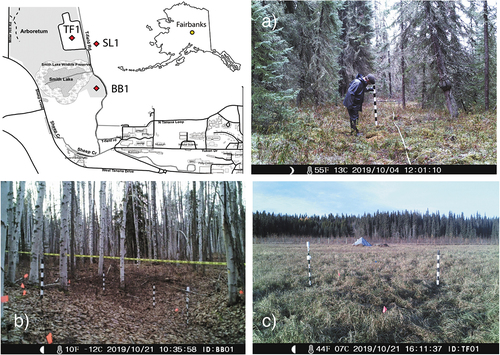
Table 2. Characteristics of the three study sites.

Index	Coordinates	Vegetation type	Specific features
SL1	64.869°N, −147.860°E	Spruce forest	Mature white spruce forest with small shrubs and moss understory: ● Trees to 20 m high with trunks 0.02 to 0.3 m. Crowns 1 to 6 m in diameter with crown projective area 1 to 30 m^2 (12 m^2 average) ● Clearings with relative area of 60% ● Total projected crown area (relative area 40%), including: ∘ Tree well bottoms (relative area 28%) ∘ Tree well slopes (relative area 12%) ● Understory of Labrador tea and Lingonberry shrubs ● Hummocky moss ground cover: 0.02 to 0.05 m microrelief
BB1	64.863°N, −147.858°E	Birch forest	Mature birch forest on relict polygonal ground; “egg carton-like” local microrelief with mounds and troughs: ● Convex polygon tops 5–10 m in diameter (relative area 80%) ● V-shaped ice wedge troughs 2 to 3 m wide (relative area 20%): ∘ Trough bottoms 1 m wide (relative area 7%) ∘ Steep trough side slopes: 10 to 35° (relative area 13%) ● Sparse grass understory
TF1	64.869°N, −147.865°E	Field with grass vegetation	Large unplowed field (250 × 350 m) with a homogeneous sedge vegetation with tussocks producing 0.02 to 0.2 m microrelief. No trees.

Methods

Sites were chosen in October. Before snow deposition, the ground surface topography was surveyed at 0.1-m intervals. Air and snow–ground interface temperature loggers (Hobo Pro v2) were installed and set to record data every 30 minutes. Game cameras (APEMAN H45) were installed and photographed the sites every 15 minutes (time-lapse mode). Multiple poles with 0.1-m black and white bands in the view of the camera were used to monitor snow depth with a resolution of 0.01 m. Wind speed at 2, 4, and 8 m was measured at a site about 2 km from the snow measurements.

At each site we observed the snow stratigraphy and properties along a 5-m (SL1, TF1) or 6-m (BB1) snow trench five times during the winter. This resulted in data being taken at least once a month starting November 20 and ending March 16. Altogether fifteen trenches were dug and during the field campaign, five at each site. At SL1 the trenches were located under mature white spruce trees with similar canopy characteristics. These trenches cut across tree wells. At BB1 the trenches were perpendicular to the ice wedge trough thalwegs between polygons in order to capture the maximum snow depth and stratigraphy variability due to the surface topography. At TF1 an area with the typical hummocky microrelief relief was selected for the trenches.

Pit and trench protocols consisted of the following: before digging a trench along a previously marked profile, a photograph of the area was made. Then the trench was dug and snow depth was measured along the trench wall at 0.1-m intervals. Visible and near-infrared photographs of the trench wall were taken with 30 percent overlap and then combined into a single panoramic image. Before photographing in the visible spectrum, the pit wall was processed with a soft brush to accentuate textural features. Layer boundaries were marked in the field and then further clarified using the photographic materials.

Measurements of snow layering, density, crystal type, form, and size were made at 1-m intervals along trenches according to the International Classification on Seasonal Snow (Fierz et al. 2009). Layer boundaries were measured to ±0.01 m. Density was measured using a 100-cc box cutter and a digital balance with an accuracy of ±10 kg/m³. To measure snow density, three samples were taken from each layer. Within a layer thicker than 0.06 m, additional samples were taken at different heights. To capture snow texture variability, hand sketches and notes were made before statistical analysis. Bulk values of snow depth and density were calculated for each trench from layer values.

The bulk snow water equivalent (SWE) was calculated from snow depth and density values measured along the trench walls. At SL1, in the forest clearings, SWE was computed from four vertical profiles in each trench, whereas for tree wells, the SWE was computed from two vertical profiles, one located near the trunk and the other near the canopy snow shedding line where snow compaction from unloading tends to be near maximum. At BB1 the polygon tops were represented by four-point measurements and trough bottoms and slopes by one and two measurements, respectively. To avoid bias when computing site-averaged snow depth, density, or SWE values, we used area weighting. To do so, we estimated the relative area of clearings (60 percent), tree well bottoms (28 percent), and slopes (12 percent) at SL1 and of polygon tops (80 percent), trough bottoms (7 percent), and slopes (13 percent) at BB1. We used the autumn surface topography and vegetation surveys for these estimates, also calculating the topographic position index (TPI; Tarca et al. 2022) and the crown radius index (CRI) for each site.

Tarca et al. (2022) used the TPI to quantify the effects of microtopography on snow depth. The index compares the elevation of each point in a data set to the mean elevation of a specified neighborhood around that point. Positive TPI values represent locations that are higher than the average of their surroundings (ridges). Negative TPI values represent locations that are lower than their surroundings (valleys).

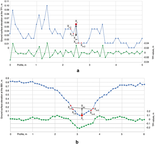
At TF1, TPI was calculated as the difference between the elevation of the central point (X_i) of each 0.4-m segment (moving along the profile at 0.1-m steps) and the average elevation (X_av) of the adjacent four points (Equations (1)(1) $\mathit{TPI}=X_i-X_{\mathit{av}},$(1) and (2(2) $X_{\mathit{av}}=\frac{1}{4}\left(X_{\mathit{i}-2}+X_{\mathit{i}-1}+X_{\mathit{i}+1}+X_{\mathit{i}+2}\right).$(2) ); Figure 2a). Points with a TPI > 0 were classified as tussock crests and points with TPI < 0 were classified as hollows between the tussocks.

(1) $\mathit{TPI}=X_i-X_{\mathit{av}},$(1)

Figure 2. (a) Snow-free surface elevation profile from TF1 showing how the topographic position index (TPI) was computed for point X_i. The topographic position index (TPI) confirms that there were five main tussock crests and three main inter-tussock lows. (b) Snow-free surface elevation profile from BB1 showing how the TPI was computed for point X_i.

where

(2) $X_{\mathit{av}}=\frac{1}{4}\left(X_{\mathit{i}-2}+X_{\mathit{i}-1}+X_{\mathit{i}+1}+X_{\mathit{i}+2}\right).$(2)

At BB1 we used a modified version of the TPI formula to capture the larger ice wedge topography features. There TPI was calculated as the difference between the elevation of the central point and a 1-m segment (moving along the profile at 0.1-m steps) and eleven adjacent points (Figure 2b). This procedure allowed us to define valley bottoms, but flat areas and long side slopes both had similar near-zero TPI values. To specify slopes and flats, we calculated the average angle between the four uttermost points of the segment (Equations (1)(1) $\mathit{TPI}=X_i-X_{\mathit{av}},$(1) and (3(3) $X_{\mathit{av}}=\frac{1}{4}\left(X_{\mathit{i}-5}+X_{\mathit{i}-4}+X_{\mathit{i}+4}+X_{\mathit{i}+5}\right).$(3) )). If the slope angle was less than 5 percent, we defined it as a flat area. If it was between 5 and 15 percent, we defined it as a gentle slope, and if it was 15 to 35 percent, we defined it as a steep slope. Thus, five classes were defined in total for BB1 (Table 3).

$\mathit{TPI}=X_i-X_{\mathit{av}},$

Table 3. Five classes defined using topographic position index (TPI) for site BB1.

TPI value	Slope	Class	Snow depth (m)	Proportion of snow depth compared to average snow depth in transect
<−0.1 m	Any	Bottom	0.65	1.12
−0.1 m to 0.1 m	5 to 15%	Side slope	0.55	0.96
−0.1 m to 0.1 m	15 to 35%	Steep side slope	0.57	0.99
−0.1 m to 0.1 m	<5%	Flat	0.56	0.98
>0.1 m	Any	Broad ridge	N/A	N/A

where

(3) $X_{\mathit{av}}=\frac{1}{4}\left(X_{\mathit{i}-5}+X_{\mathit{i}-4}+X_{\mathit{i}+4}+X_{\mathit{i}+5}\right).$(3)

At SL1, where the effect of conifer trees was strong but the microtopography limited, we use the CRI to quantify the effect of conifer crowns on snow properties. This index is based on an idea presented by Hardy and Albert (1995) where they divided the area radially out from a tree trunk into four zones. Their Zone 1, immediately adjacent to the trunk, occupied only 0.3 percent of their test area, so we exclude it, reducing the classification down to three zones (Table 4). CRI-1 is the zone from R = 0 to R = 0.5R_cr (where R_cr is the radius of the tree crown) and largely defines the area under the canopy where the snow is greatly depleted. CRI-2 is the annulus from R = 0.5R_cr to R = 1.2R_cr that defines the most disturbed and heterogeneous area of snow near the canopy shed line. R > 1.2R_cr is the area beyond the influence of one tree but before a second tree influence is encountered.

Table 4. Crown radius index (CRI) indices and their locations.

CRI	Criteria	Class
1	The area from the tree trunk to the edge of the crown with radius R = 0.5Rcr	Tree well bottom
2	The circle area around the edge of the crown with R = 0.5Rcr and R = 1.2Rcr	Tree well slope
3	The area between 1.2Rcr of the two adjacent trees	Forest clearing

Experiment data

We analyzed meteorological data and the results of remote and manual snow measurements to explore how local controls alter the spatial variability of the taiga snow cover. By choosing sites located close together, we eliminated between-site variations due to snowfall and weather, allowing us to focus on how local topography and vegetation affected the snow distribution. To quantify local topography and vegetation differences, we used TPI and CRI, as well as descriptive measures. To quantify the response of the snow cover, we measured the variability of snow depth, density, SWE, and stratigraphy in long trenches. Consistent with prior work, we expected that the strongest influence on the local snow distribution would be the interception of snow by the forest canopy, with the ground topography having the second strongest effect. Those findings, though important, are not novel. But the end-result snow cover in the taiga is always the product of overlapping and interacting processes, so modeling or predicting the local snow distribution has been an elusive goal. Here, we provide an approach to how this might be done, and that approach is new.

Weather conditions and bulk snow properties

The 2019–2020 winter had climatologically normal temperatures but slightly above-average snowfall for Fairbanks (Table 5). The average November to May air temperature was −16°C, with periods in December through February seeing temperatures as low as −35°C (Figure 3). Despite these low temperatures, throughout the winter, snow–ground interface temperatures did not drop below −4°C, producing at times vertical temperature gradients as high as 110°C/m, driving the intensive depth hoar metamorphism characteristic of the taiga snow cover. Much of the buildup of the snowpack took place in November and again in March. The maximum snow depth, about 0.80 m, was observed at the end of March, with the average snow depth in March being 0.66 m.

Figure 3. Meteorological data from the three sites. Air and snow–ground interface temperatures were nearly the same at the sites, despite differences in the nature of the ground vegetation.

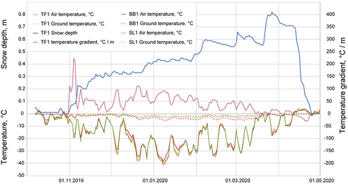
Table 5. Average November to May Fairbanks air temperature and March snow depth, 1930–2020 versus 2019–2020.

Year	Average air temperature (November to May)	Average snow depth in March
1930–2020	−15°C	0.61 m
2019–2020	−16°C	0.66 m

The bulk snow density was similar but not identical at all three sites throughout the winter. It increased slowly from 160 kg/m³ in November to 180 kg/m³ in January to peak values of 190 kg/m³ in March. The limited densification can be attributed to the fact that most of the pack was depth hoar (e.g., faceted crystals; 60 percent), with some limited rounded grains (35 percent) and fresh snow (5 percent). Kojima (1956) and Akitaya (1974) have documented the “stiffness” of depth hoar under compression. The pack also underwent virtually no insolation melt due to the low values of incoming solar radiation in Fairbanks in winter (Bowling 1986). The wind speed was also low, with winter average values of about 0.2 m/s. This eliminated wind transport at BB1 and SL1 and limited it greatly at TF1. Air and snow–ground interface temperatures were nearly identical at the three sites, despite differences in the nature of the ground vegetation (Figure 3). Therefore, any differences in temperature gradients across the snow cover were the result of differences in snow depth and the nature of the snow.

Consistent with canopy interception, early in the winter the lowest SWE was found at SL1, whereas the highest was at TF1. Though we cannot confirm that TF1 SWE represents the total amount of snowfall for all three sites, we can assume that it is close to that value. Because any wind transfer is local and short distance and sublimation from trees is diminished in the study area (Sturm 1992), comparing the bulk SWE at BB1 and SL1 with TF1 suggests that early in the winter 11 mm (or 20 percent of what had fallen) was lodged in the conifer canopy at SL1, whereas 6 mm (or 11 percent of what had fallen) was lodged in branches of the deciduous trees at BB1. As winter progressed, snow cascading from the trees slightly reduced these differences.

Variability of snow properties in trenches

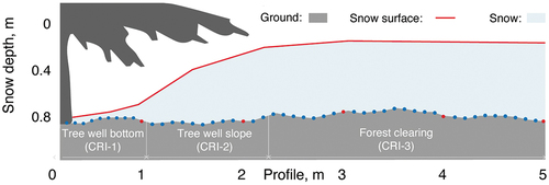
At SL1, snow interception, unloading, and other processes led to snow depletion beneath the canopy and enhanced depth, density, and SWE just outside the edge of the canopy. The three CRI-defined classes of terrain had distinctly different snow regimes. In areas adjacent to the tree trunks (CRI-1), the snow depth only marginally increased through the season, whereas from 1 m out (CRI-2, CRI-3) it continued to increase (Figure 4). At the bottoms of tree wells, the snow depth was 74 percent lower and the density 7 percent lower than in the adjacent forest clearings, resulting in a 76 percent depletion of tree well SWE by mid-March. At the outer radius of the tree wells (the well slope: CVI-2), the snow cover was disturbed and compacted by snow masses unloaded from branches. In places density exceeded 350 kg/m³ by mid-winter. The average snow depth was 17 percent smaller, but the density was 50 percent higher in this area than in the adjacent clearings, making the bulk SWE 25 percent higher than in clearings. The deepest and most homogeneous snow was observed in forest clearings, where the snow cover was not affected by conifer canopies. The effect of shrub vegetation and ground microtopography was limited there and resulted in less than 10 percent variability of snow depth, density, and SWE, which is consistent with the variability of these parameters at the field site.

Figure 4. Snow depth in tree wells and adjacent forest clearings in the spruce forest (SL1) in March. The difference in snow depth in tree wells (Crown radius index (CRI)-1, 2) versus clearings (CRI-3) continued to increase with each additional snowfall due to snow interception and unloading from tree crowns. Blue dots = snow depth measurements; red dots = snow density and snow water equivalent (SWE) measurements during trench excavation.

The combination of local vegetation and microtopography factors resulted in more than 45 percent variation of SWE at the site by mid-March, several times more than at BB1 and TF1 sites. Thus, though low vegetation could be found in the clearings, as well as some microtopography, the dominant control at SL1 on the snow distribution was crown interception.

Compared to SL1, at BB1 the effect of snow interception by branches was more limited and more transient but still measurable. Snow was not retained on canopies for more than five to seven days and cascaded from leaf-bare branches in a random manner causing little densification. Unlike SL1, no tree wells formed. On thicker branches (more than 0.05 m in diameter) and on strongly inclined tree trunks, snow was retained for up to several weeks, resulting in a slight reduction of snow depth and SWE beneath these features compared to open sites (Table 6). Fallen dead trees, logs, and vertical trunks had a marked effect on the snow depth and SWE distribution at a submeter scale but were limited in area to just a few percent of the total snow area at the site (perhaps accounting for 2–3 percent of the snow variations).

Table 6. Area-weighted snow depth, density, and snow water equivalent (SWE) and their variability at the three sites. The SL1 clearing column represents an area of undisturbed snow in forest clearings outside the tree wells.

	BB1		TF1		SL1		SL1 clearing
Date	Depth (m)	Variability (%)	Depth (m)	Variability (%)	Depth (m)	Variability (%)	Depth (m)	Variability (%)
Snow depth
20 November	0.33	6	0.34	8	0.27	31	0.31	9
10 December	0.32	5	0.35	7	0.26	38	0.32	8
13 January	0.42	6	0.46	5	0.34	38	0.44	5
18 February	0.49	6	0.54	5	0.43	39	0.54	6
16 March	0.56	6	0.62	3	0.52	35	0.61	4
Snow density
20 November	160	6	159	9	166	12	160	3
10 December	180	7	175	3	173	11	173	3
13 January	180	6	176	4	176	15	179	4
18 February	175	10	180	2	198	24	180	4
16 March	185	7	188	3	198	22	181	4
SWE
20 November	48	6	54	10	43	26	47	9
10 December	56	7	61	7	50	27	54	7
13 January	66	12	81	8	68	28	69	8
18 February	85	13	96	3	85	42	96	8
16 March	106	12	119	5	101	45	112	9

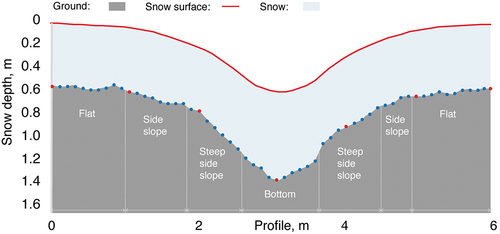
However, the presence of the steep thermokarst topography at BB1 increased the variability of snow cover at this site (Figure 5, Table 6). Due to downslope settlement of the snow on the steep sides, trough bottom snow was 12 percent deeper and 14 percent denser than on adjacent polygon tops by mid-March (Figure 5). On the steep side slopes of the troughs, where the snow cover had been “stretched,” snow depth and density were slightly lower than on polygon tops. The end result of this gravitational-driven settlement was that the maximum SWE at trough bottoms was 28 percent higher than on the polygon tops and 31 percent higher than on trough side slopes less than 1 to 2 m away. These differences were more accentuated the deeper and steeper the trough. Surprisingly, despite snow accumulation taking place in calm conditions at this site, lateral variations in depth and density driven by the steep topography produced heterogeneity that approached levels often measured in wind-blown tundra snow (Sturm and Benson 2004).

Figure 5. Snow depth distribution in the birch forest (BB1) in March. Deeper snow accumulated in the thermokarst troughs (bottom) compared to polygon tops (flat), and this difference increased during the winter. Blue dots = snow depth measurements; red dots = snow density and snow water equivalent (SWE) measurements.

At TF1, where no trees were present, grass tussocks altered the snow properties and stratigraphy. Deeper and denser snow accumulated between tussocks due to creep and some wind transfer, whereas on the tussock’s convex crests, the snow was thinner and softer. This difference increased with increasing height of tussocks. Lateral variability in depth, density, and SWE did not exceed 10 percent, consistent with the background variability of the ground cover and quantified by the low TPI values we computed (Figure 6). This variability decreased with increasing snow depth due to relief smoothing (Table 6, Figure 7; cf. Filhol and Sturm 2019). By the time the snow depth reached 0.3 m in mid-November at TF1, the microtopography no longer produced any surface expression, with the snow surface smooth and uniform across the site.

Figure 6. Snow depth distribution at the TF1 field site in March. Over the convex tussock crests, the snow was thinner compared to areas between tussocks. This resulted in snow depth lateral variability, which decreased with additional snowfall from 8 to 3 percent. Blue dots = snow depth measurements; red dots = snow density and snow water equivalent (SWE) measurements.

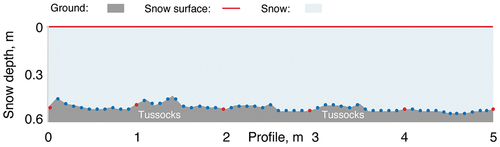
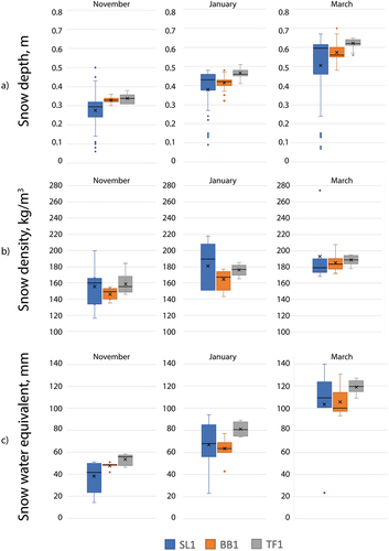
Figure 7. Box plots of average (a) snow depths, (b) density, and (c) snow water equivalent (SWE) measured along 5-m (SL1 and TF1) and 6-m (BB1) profiles in November, January, and March. Snow depth was measured at 0.1-m intervals. Bulk snow density and SWE were measured at 1-m intervals (n = 6–7). At SL1 and BB1 forest sites, the variability in snow properties increased with additional snowfall, whereas at the TF1 field site it decreased during the winter. The outliers at the SL1 site in March represent the areas of snow depletion under tree crowns and areas of snow compaction by unloaded snowballs.

Due to wind exposure, slab layers formed occasionally at TF1, with local density values as high as 350 kg/m³, twice the average density of the layers at the two forest sites. Lateral variability of density and SWE of these wind slab layers was on average 20 percent, up to five times more than layers accumulated in windless conditions. At times, the snow surface was covered by very small dunes and other eolian forms, which were absent in the two forest sites. Applying the TPI, we were able to determine that the average snow depth on the crests was 4 percent lower than that measured between tussocks, whereas the snow density and SWE were 3 percent (density) and 5 percent (SWE) lower than between tussocks.

Thus, by mid-March the average spatial variability of SWE at the SL1 site was 45 percent. Separating how much of this was due to canopy interception and redistribution versus microtopography is difficult. We have made qualitative estimates by extrapolating measured variations in SWE away from tree canopies and comparing them to the SWE variations where canopies added to the variance. This compare-and-contrast approach suggests that 35 percent of the SWE variance was canopy driven, with an additional 10 percent variability the result of ground shrubs and vegetation-driven microtopography. Combined, the overall spatial variability due to vegetation and microtopography was 45 percent at this site. At the field site (TF1), the SWE variability was 5 percent by mid-March, the result of surface microtopography and snow redistribution by wind. At the deciduous forest site (BB1), the SWE spatial variability due to settlement in thermokarst troughs was estimated as 10 percent, with an additional 2 to 3 percent variability due to vegetation-driven microtopography by mid-March. In summary, snow interception and unloading from canopy were the strongest agents in producing snow depth and SWE heterogeneity, several times stronger than sharp microtopography or tussock/hummock relief.

Variability of snow stratigraphy in trenches

Though the area-averaged depth and SWE were nearly the same from site to site (Figure 7), the stratigraphy was uniquely different. The processes (unloading, settlement, etc.) that produced spatial variations in depth and SWE tended to be conservative in the sense that they resulted in nonunique snow depth and SWE outcomes by site, but the stratigraphic and textural outcomes were distinctive, particularly when an entire site was considered. Figure 8 shows these salient stratigraphic differences.

Figure 8. The stratigraphy of mature snow at the three sites. Despite the overall similarities in snow depth, density, and snow water equivalent (SWE) by March, the stratigraphy at the three sites was quite different. At the TF1 field site, wind slab layers formed. On the tussock’s crests (1), snow layers were thinner and softer compared to areas between tussocks (2). Extensive hollows up to 0.1 × 0.5 m associated with bunches of prostrate grass were observed. At SL1, snow layers at the bottoms of tree wells (3) were three to five times thinner than in forest clearings (5), and interfaces between layers were difficult to detect within the wells. At the edge of the canopies (4), the original snow stratigraphy was strongly disturbed by dense snowballs that had fallen from the trees. Voids and cavities formed around small conifers (6) and buried understory vegetation (7) and depth hoar textures were limited due to diminished kinetic growth metamorphism. At BB1, cones of snow and cavities formed around tree trunks (8). At the bottoms of troughs (9), snow was deeper and denser, and the kinetic growth was diminished, in contrast to thinner and more fragile areas of snow on steep side slopes (10). On logs and fallen trees (11), snow layers were thinner and stratigraphy was better preserved compared to adjacent areas around logs (12). Snow cover was disturbed by snowballs and rolls from canopy in a random manner and did not change snow stratigraphy considerably.

Overall, the stratigraphic findings again show that conifer canopies had the strongest effects (through interception and unloading), effects that increased through the season. Deciduous trees and shrub vegetation had measurable, but relatively smaller, effects due to the limited projection area and strength of branches. Nevertheless, these branches still influenced the snow stratigraphy around trunks and buried stems. Sharp surface microtopography had the second strongest effect after canopies and influenced the snow variability through initial depositional (creep and saltation) and postdepositional (settlement) snow process. The snow variability due to grass tussocks was limited and decreased with additional accumulation due to strong relief smoothing, whereas large thermokarst troughs continued to increase the variability during the winter (Table 6, Figure 7).

A four level model of snow heterogenization

There are many papers (Table 1) on the topic of taiga snow depth and SWE heterogeneity but no universal or general method of dealing with these variations because of the complex and overlapped nature of the processes that produce heterogeneity. That difficulty is compounded by the fact that most of these processes operate at similar spatial–temporal scales (Table 6, Figures 7 and 8). However, stratigraphy produced by the interaction of the snow and local vegetation tends to be unique. For example, local vegetation and microtopography produce distinctly different cross sections that can be ascribed to specific taiga settings (Figure 8). So, although we cannot yet implement a general solution for taiga snow distribution, we can start to recognize snow outcomes and their relationships to the various taiga subenvironments.

To that end, we present a conceptual framework for understanding taiga snow variability. It has four vertical levels of snow–vegetation–microtopography interactions (Table 7), and considers trees, shrubs, microtopography, and soil as filters that either enhance or diminish internal snow stratigraphy, snow depth, and density in predictable ways (Figure 8).

Table 7. The four levels of influence for taiga snow.

Level	Control	Result
Above canopy	Climate: precipitation, temperature, wind, solar radiation, humidity	Same above-canopy weather conditions should produce the same snow stratigraphy
In canopy: ●Trees ●Shrubs	Vegetation: species, age, size, morphology, density	Wind and insolation shading, snow interception and redistribution through unloading alter snow properties
On the ground	Microtopography: wavelength, amplitude	Snow rebound, creep, and settlement toward troughs additionally increase snow variability
Belowground	Ground and soil: composition, moisture, temperature	Variable heat and mass fluxes from soil result in uneven snow metamorphism

Over small (<5 km) distances, for terrain that has little variation in altitude or aspect (like our study), above-canopy weather conditions are unlikely to differ significantly; hence, that level can be ignored. Similarly, though the filtering effect continues at the lowest level with processes controlled by belowground conditions (e.g., moisture and heat fluxes that impact snow metamorphism), we do not address those here because they were not considered in our study.

The filtering process begins in the canopy if one is present (Tables 7 and 8). It will alter local weather conditions, snow accumulation, and metamorphism processes by (1) a reduction in wind and insolation due to tall vegetation and (2) interception and unloading of snow from the canopy. Because wind speed is reduced in forests, no wind slabs form and little long-distance snow transfer occurs, unlike in open areas. Interception of snow in the canopy results in snow depletion under trees and formation of tree wells in conifer forests, and snow unloading from branches densifies snow and disturbs the original stratigraphy. Canopy in the deciduous forests plays a more limited role and results only in slight reduction of the SWE but considerably different site stratigraphy (Figure 8).

Table 8. Filtering effects of canopy and microtopography.

		Accumulation			Metamorphism
Site	Site description	Above canopy	In canopy	On the ground	Above canopy	In canopy	On the ground
TF1	Large field with grass tussocks No trees	Same weather conditions produced the same input across all sites	No trees and shrubs: ● Strong wind; Wind slab layers ● Aeolian microrelief on snow surface	Grass tussocks: ● Deepand dense snow between tussocks ● Shallowand loose snow on tussock crests ● Voids and cavities around grass patches	Same weather conditions produced the same input across all sites	X	Grass tussocks and wind slab layers influence depth hoar metamorphism rates
BB1	Birch forest with thermokarst troughs		Deciduous trees and no shrubs: Some wind reduction Some canopy interception ● No tree wells ● Limited SWE reduction	Thermokarst troughs: ● Deepand dense snow in troughs ● Shallowand loose snow on steep slopes ● Uneven snow accumulation near logs and tree trunks		Snow masses unload from deciduous trees: ● Limited and random densification of snow ● Small effect on snow metamorphism	Uneven snow distribution in troughs, near tree trunks and logs alter depth hoar metamorphism
SL1	White spruce forest with moss cover and small shrubs understory		Conifer trees and shrubs intercept snow: Strong wind reduction ● Deep and homogeneous snow in clearings ● Strong canopy interception; hence SWE reduction ● Tree wells under canopies ● Voids and cavities around buried shrubs	Moss hummocks: ● Deeper snow between moss hummocks than on crests due to creep		Snow masses unload from conifer trees: ● Strong snow densification around canopies ● Uneven snow metamorphism and disturbed stratigraphy under canopies	Tree wells, moss hummocks, shrubs, tree trunks, and logs alter depth hoar metamorphism

Note. SWE = snow water equivalent.

Understory vegetation continues to “filter” or alter snow properties and stratigraphy around voids and cavities that form under the buried plants (Figures 4 and 8). It does so mainly by creating heat flow pathways that reduce gradients, thereby diminishing kinetic growth metamorphism (Sturm 1992).

The presence of distinct on-the-ground microtopography continues the “filtering” process, changing the snow spatial variability regardless of the presence of tree vegetation. The effect of surface microtopography on snow distribution during and after deposition may be strong enough to add to structural variability. It depends on the surface wavelength, amplitude, and roughness of the microtopography. Deeper and denser snow accumulates in concave microrelief, an effect that is enhanced where slopes are steeper (Figures 5 and 8). Where slopes are less steep or flat, snow smoothing occurs (Filhol and Sturm 2019), an effect that is more pronounced when there is snow redistribution by wind (but not enough wind to create dunes).

Discussion

How might we model snow heterogeneity using the filter concept (Tables 7 and 8), and why would we want to do so? Snow cover models are widely used for avalanche forecast and ecosystem research (Brun et al. 1989; Durand et al. 1999; Endrizzi, Quinton, and Marsh 2011; Krogh, Pomeroy, and Marsh 2017). These generally model the snow stratigraphy and properties at a single point but, as we have documented here, considerable heterogeneity even at small scales produces inconsistencies between model calculations and in situ measurements. The heterogeneity could be explicitly modeled or dealt with statistically using the functional relationships between snow stratigraphy, depth, and SWE and filter elements listed and described above. Using either measured or inferred vegetation and microtopography data, maps of snow properties could then be drawn over base maps of vegetation and microtopographic data. Average values could be produced by integrating these inferred properties across the domain. Such an approach should work because of the strong relationships between taiga forest characteristics, microtopography, and the resulting snow cover (Figures 8 and 9).

Figure 9. Areas with specific snow characteristics and stratigraphy due to local factors: (a) plan view (from top) and (b) schematic profile of snow cover along the red line. At the tree well bottoms (CRI-1), the snow depth, density, and snow water equivalent (SWE) are strongly reduced and the depth hoar is better developed than in forest clearings (CRI-3), whereas at the tree well slopes (CRI-2), snow cover is compressed and disturbed by unloading snow. Above tussock crests (points with positive topographic position index (TPI) values), snow depth, density, and SWE are smaller and the wind slab layers are less developed than between tussocks (points with negative TPI values). Trough bottoms, represented by points with negative TPI values, snow depth, density, and SWE is bigger, and the depth hoar is less developed compared to polygon tops.

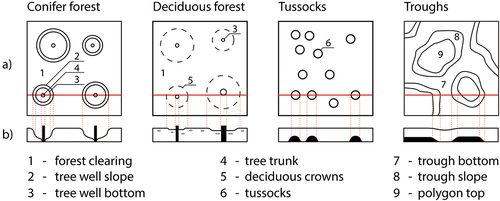
To illustrate this idea, consider the four trees shown in Figure 9 (left panel), each of crown radius R_i. From Figures 4 and 8 and Table 6, the CRI would allow us to define bagel-like areas of snow with specific snow characteristics, and where these bagel areas are intersected, adjustments would be made. A similar approach (next panel) could be applied to deciduous trees. The same approach should even be possible for surface microtopography (third and right panels) if microtopographic data could be obtained, by using TPI parameters.

We have created a simple set of filter rules in Table 9. At this point, we cannot go beyond this simple breakdown into snow variations that are “below,” “above,” or “average,” but refinements could readily be done with more data. Adapting snow codes by applying the concept in Table 9 could enable contemporary climate models, which usually have low spatial resolution, to quantify the effect of sub-grid-scale variability of, for example, snow microstructure and properties at larger scales (Todt 2019). To assess how well the climate models perform, the results of in situ measurements would be required. Because detailed in situ measurements are sparse, the conceptual model could be applied to improve the results of satellite remote sensing, which is used for verification of land surface models within forecast schemes and monitoring of global snow resources (Takala et al. 2011).

Table 9. Filter rules affecting snow depth, density, SWE, and stratigraphy in Alaskan taiga.

Level	Filter	Control	Subarea	Depth	Density	SWE	Stratigraphy
In canopy	Vegetation	Conifer trees	In tree well bottoms	−	−	−	Extreme depth hoar
			On tree well slopes	−	++	+	Disturbed stratigraphy by unloading snowballs
			In forest clearings	+	=	=	Uniform undisturbed stratigraphy with no wind slab layers
		Deciduous trees	Below trees	−	=	−	Uniform stratigraphy with few random unloading marks
		Shrubs and grass patches	Above low vegetation	−	=	−	Voids and cavities around buried plants
On the ground	Topography	Troughs	At the bottoms	+	+	+	Compacted snow with thick layers and limited depth hoar
			On slopes	−	−	−	Loose snow with thinker depth hoar layers
			On polygon tops	=	=	=	Uniform undisturbed stratigraphy with few wind slab layers in forest clearings
		Tussocks and hummocks	Above crests	−	−	−	Thin and loose snow layers with limited wind compaction
			Between tussocks	+	+	+	Thick and hard snow layers compacted due to wind

Note. +above average; –below average; =site average. SWE = snow water equivalent.

The concept could help to further develop SWE remote sensing methods (Kelly et al. 2003; Rutter et al. 2019) because the layering of the snow has a strong effect on the absorption and reflection of microwave radiation by the snow (Josberger and Mognard 2002; Golubev, Petrushina, and Frolov 2010). Retrievals that incorporate estimates of the snow stratigraphy perform better than those that do not (King et al. 2018; Meloche et al. 2022). Thus, the understanding of snow stratigraphy variability due to local factors is a key to identifying and decomposing backscatter contributions at scales smaller than 10 m and to accurately estimating SWE. Modern airborne technologies (lidar, unmanned aerial vehicle photogrammetry) allow derivation of detailed digital models of the ground and snow surface topography with better than 0.1-m vertical resolution (Bühler et al. 2015; Nolan, Larsen, and Sturm 2015; Mazzotti et al. 2019); however, measuring snow beneath forest vegetation canopy is still a challenge (Deems et al. 2013), and these surficial measurements cannot distinguish individual snow layering (Marshall, Schneebeli, and Koh 2007). Better models could help to fill this gap.

Conclusion

Observations of snow depth, density, SWE, and stratigraphy at the three sites (birch forest, white spruce forest, grass field) with distinctly different local microtopography and radically different vegetation were made near Fairbanks, Alaska. Despite the same winter weather conditions above tree canopies, the snow properties and stratigraphy were quite different at the three sites due to local factors related to depth distribution and metamorphism. Widely different canopy interception processes proved to have the strongest impact on the resulting snow cover heterogeneity. Surface microtopography had the second strongest effect on the local snow variability through depositional and postdepositional processes. Ultimately, these factors will need to be separated to quantify their contribution to site-specific taiga snow characteristics.

By studying the three sites, we observed the following:

1. Tree canopies intercepted snow and disturbed ground snow structure through a series of capture and unloading events. These processes caused a reduction of snow depth, density, and SWE under the canopy in the spruce forest and a slight reduction in places in the birch forest compared to open areas. Under conifers tree wells formed, whereas in deciduous forest this effect was more random.

2. Trees reduced wind considerably, so more homogeneous snow was found in forest clearings than in open fields, where wind slab layers formed occasionally.

3. Steep, sharp microtopography (thermokarst ice wedges) increased the variability of snow cover through gravitational settlement, with the SWE in thermokarst troughs about 30 percent greater than that on tops of adjacent polygons by the end of the winter.

4. Tussock microtopography and logs made an irregular surface that created deeper snow in hollows and thinner snow on crests.

5. Understory vegetation (shrubs, grasses, sedges, moss) formed a system of cavities at the base of the snow cover. The background variability due to sub-meter-scale microrelief and understory vegetation was small but measurable.

6. Local factors produced similar snow depth, density, and SWE at our three sites but radically different stratigraphy.

7. It appears to us that local vegetation and microtopography factors could be separated in order to quantify their contribution to the overall stratigraphic and depth outcomes.

We conceptually parameterize the findings by applying a set of rules driven by these local factors, suggesting that the resulting model could be used to isolate the effects of local factors on taiga snow. By separating these local factors, it should be possible to improve the modeling of the snow outputs resulting from any combination of vegetation and microtopography, which could strongly vary even within a small area at submeter scales. This approach could be applied to improve the accuracy of global climate models, the quality of forecasts, the results of remote sensing, and snow modeling.

Acknowledgments

Instrumentation for the field sites was generously loaned to us by A. Kholodov. A. Pinzner, B. Sturm, and A. Belousova helped in the field. V. Romanovsky and colleagues at the Geophysical Institute (University of Alaska, Fairbanks) provided encouragement and support. S. Sokratov and his colleagues at the Laboratory of Snow Avalanches and Debris Flows (Lomonosov Moscow State University) supported us with comprehensive assistance and fruitful discussion.

Disclosure statement

No potential conflict of interest was reported by the authors.

Additional information

Funding

This collaboration was made possible by a Fulbright grant to AK.

References

- Akitaya, E. 1974. Studies on depth hoar. Contributions from the Institute of Low Temperature Science 26:1–18.
- Barry, R., M. Prévost, J. Stein, and A. P. Plamondon. 1990. Application of a snow cover energy and mass balance model in a balsam fir forest. Water Resources Research 26 (5):1079–92. doi:10.1029/WR026i005p01079.
- Benson, C. S. 1969. The seasonal snow cover of arctic Alaska, 1–47. Washington, Arctic Institute of North America.
- Benson, C. S., and D. C. Trabant. 1973. Field measurements on the flux of water vapor through dry snow. Proceedings: Symposium on the Role of Snow and Ice in Hydrology, 291–98. doi:10.5194/tcd-6-1673-2012.
- Bowling, S. A. 1986. Climatology of high-latitude air pollution as illustrated by Fairbanks and Anchorage, Alaska. Journal of Climate and Applied Meteorology 22-34.
- Brun, E., Ε. Martin, V. Simon, C. Gendre, and C. Coleou. 1989. An energy and mass model of snow cover suitable for operational avalanche forecasting. Journal of Glaciology 35 (121):333–42. doi:10.3189/S0022143000009254.
- Bühler, Y., M. Marty, L. Egli, J. Veitinger, T. Jonas, P. Thee, and C. Ginzler. 2015. Snow depth mapping in high-alpine catchments using digital photogrammetry. The Cryosphere 9 (1):229–43. doi:10.5194/tc-9-229-2015.
- Bunnell, F. L., R. S. McNay, and C. C. Shank. 1985. Trees and snow: The deposition of snow on the ground. A Review and Quantitative Synthesis. Research Branch, British Columbia Ministries of Environment and Forests, Victoria Research. Paper no. IWIFR-17.
- Chapin, F. S., III, K. van Cleve, and M. C. Chapin. 1979. Soil temperature and nutrient cycling in the tussock growth form of Eriophorum vaginatum. The Journal of Ecology 169–89. doi:10.2307/2259343.
- Davis, R. E., J. P. Hardy, W. Ni, C. Woodcock, J. C. McKenzie, R. Jordan, and X. Li. 1997. Variation of snow cover ablation in the boreal forest: A sensitivity study on the effects of conifer canopy. Journal of Geophysical Research 102 (29):389–29. 396. doi:10.1029/97JD01335.
- Deems, J. S., T. H. Painter, and D. C. Finnegan. 2013. Lidar measurement of snow depth: A review. Journal of Glaciology 59 (215):467–79. doi:10.3189/2013JoG12J154.
- Domine, F., A. Taillandier, S. Houdier, F. Parrenin, W. R. Simpson, and T. A. Douglas. 2006. Interactions between snow metamorphism and climate: Physical and chemical aspects. Special Publication-Royal Society of Chemistry 311:27.
- Durand, Y., G. Giraud, E. Brun, L. Mérindol, and E. Martin. 1999. A computer-based system simulating snowpack structures as a tool for regional avalanche forecasting. Journal of Glaciology 45 (151):469–84. doi:10.3189/S0022143000001337.
- Endrizzi, S., W. L. Quinton, and P. Marsh. 2011. Modelling the spatial pattern of ground thaw in a small basin in the Arctic tundra. Cryosphere 5:367–400. doi:10.5194/tcd-5-367-2011.
- Faria, D. A., J. W. Pomeroy, and R. L. H. Essery. 2000. Effect of covariance between ablation and snow water equivalent on depletion of snow‐covered area in a forest. Hydrological Processes 14 (15):2683–95. doi:10.1002/1099-1085(20001030)14:15<2683::.
- Fassnacht, S. R., and J. S. Deems. 2006. Measurement sampling and scaling for deep montane snow depth data. Hydrological Processes 20 (4):829–38. doi:10.1002/hyp.6119.
- Fierz, C. R. L. A., R. L. Armstrong, Y. Durand, P. Etchevers, E. Greene, D. M. McClung, K. Nishimura, et al. 2009. The international classification for seasonal snow on the ground. UNESCO. https://unesdoc.unesco.org/ark:/48223/pf0000186462
- Filhol, S., and M. Sturm. 2019. The smoothing of landscapes during snowfall with no wind. Journal of Glaciology 65 (250):173–87. doi:10.1017/jog.2018.104.
- Formozov, A. N. 1946. Snow cover as an integral factor of the environment and its importance in the ecology of mammals and birds. Fauna and Flora of the USSR. Zoological Institute. New series, 5, 1–152. CRREL Acc. No: 04004702
- Gelfan, A. N., J. W. Pomeroy, L. S., and K. 2004. Modeling forest cover influences on snow accumulation, sublimation, and melt. Journal of Hydrometeorology 5 (5):785–803.
- Golding, D. L., and R. H. Swanson. 1986. Snow distribution patterns in clearings and adjacent forest. Water Resources Research 22 (13):1931–40. doi:10.1029/WR022i013p01931.
- Golubev, V. N., M. N. Petrushina, and D. M. Frolov. 2010. Development patterns of snow cover stratigraphy. Ice and Snow 1.
- Hardy, J. P., and M. R. Albert. 1995. Snow‐induced thermal variations around a single conifer tree. Hydrological Processes 9 (8):923–33. doi:10.1002/hyp.3360090808.
- Hardy, J. P., R. E. Davis, R. Jordan, X. Li, C. Woodcock, W. Ni, and J. C. McKenzie. 1997. Snow ablation modeling at the stand scale in a boreal Black pine forest. Journal of Geophysical Research 102 (29):397–407. doi:10.1029/96JD03096.
- Hedstrom, N. R., and J. W. Pomeroy. 1998. Measurements and modelling of snow interception in the boreal forest. Hydrological Processes 12(10‐11):1611–25. doi:10.1002/(SICI)1099-1085(199808/09)12:10/11<1611::.
- Josberger, E. G., and N. M. Mognard. 2002. A passive microwave snow depth algorithm with a proxy for snow metamorphism. Hydrological Processes 16 (8):1557–68. doi:10.1002/hyp.1020.
- Jost, G., M. Weiler, D. R. Gluns, and Y. Alila. 2007. The influence of forest and topography on snow accumulation and melt at the watershed-scale. Journal of Hydrology 347 (1–2):101–15. doi:10.1016/j.jhydrol.2007.09.006.
- Kelly, R. E., A. T. Chang, L. Tsang, and J. L. Foster. 2003. A prototype AMSR-E global snow area and snow depth algorithm. IEEE Transactions on Geoscience and Remote Sensing 41 (2):230–42. doi:10.1109/TGRS.2003.809118.
- King, J., C. Derksen, P. Toose, A. Langlois, C. Larsen, J. Lemmetyinen, M. Sturm, B. Montpetit, A. Roy, and N. Rutter. 2018. The influence of snow microstructure on dual-frequency radar measurements in a tundra environment. Remote Sensing of Environment 215:242–54. doi:10.1016/j.rse.2018.05.028.
- Kojima, K. 1956. Viscous compression of natural snow-layer II. Low Temperature Science 15:117–35.
- Kokelj, S. V., and M. T. Jorgenson. 2013. Advances in thermokarst research. Permafrost and Periglacial Processes 24 (2):108–19. doi:10.1002/ppp.1779.
- Komarov, A. Y., Y. G. Seliverstov, P. B. Grebennikov, and S. A. Sokratov. 2018. Spatio-temporal heterogeneity of the snow cover from data of the penetrometer SnowMicroPen. Ice and Snow 58 (4):473–85. (In Russ.). doi:10.15356/2076-6734-2018-4-473-485.
- Komarov, A. Y., Y. G. Seliverstov, P. B. Grebennikov, and S. A. Sokratov. 2019. Spatial variability of snow water equivalent–the case study from the research site in Khibiny Mountains, Russia. Journal of Hydrology and Hydromechanics 67 (1):110–12. doi:10.2478/johh-2018-0016.
- Kopanev, I. D. 1978. Snezhnyy pokrov na territorii SSSR [Snow cover in the USSR]. Gidrometeoizdat, Leningrad, 181pp. In Russian with English table of contents enclosed. 48 refs. CRREL Acc. No: 34000846
- Kotlyakov, V. M., A. V. Sosnovsky, and R. A. Chernov. 2019. Influence of the snow–soil contact conditions on the depth of ground freezing (based on observations in the Kursk region). Ice and Snow 59 (2):182–90. (In Russ.). doi:10.15356/2076-6734-2019-2-407.
- Krogh, S. A., J. W. Pomeroy, and P. Marsh. 2017. Diagnosis of the hydrology of a small Arctic basin at the tundra-taiga transition using a physically based hydrological model. Journal of Hydrology 550:685–703. doi:10.1016/j.jhydrol.2017.05.042.
- Kuz’min, P. P. 1957. Physical processes within a snow cover. Fizicheskie Svoistva Snezhnogo Pokrova, Gidrometeoizdat, Leningrad, 11-26. CRREL Acc. No: 14017477
- Kuz’min, P. P. 1961. Melting of snow cover, 290. Israel Program for Scientific Translation: Jerusalem.
- Kuz’min, P. P. 1963. Snow cover and snow reserves: Translated from Russian, 140. Jerusalem: Israel Program for Scientific Translations.
- Loranty, M. M., S. J. Goetz, and P. S. Beck. 2011. Tundra vegetation effects on pan-Arctic albedo. Environmental Research Letters 6 (2):024014. doi:10.1088/1748-9326/6/2/029601.
- Marshall, H. P., M. Schneebeli, and G. Koh. 2007. Snow stratigraphy measurements with high-frequency FMCW radar: Comparison with snow micro-penetrometer. Cold Regions Science and Technology 47 (1–2):108–17. doi:10.1016/j.coldregions.2006.08.008.
- Mazzotti, G., W. R. Currier, J. S. Deems, J. M. Pflug, J. D. Lundquist, and T. Jonas. 2019. Revisiting snow cover variability and canopy structure within forest stands: Insights from airborne lidar data. Water Resources Research 55 (7):6198–216. doi:10.1029/2019WR024898.
- Meloche, J., A. Langlois, N. Rutter, A. Royer, J. King, B. Walker, and E. J. Wilcox. 2022. Characterizing Tundra snow sub-pixel variability to improve brightness temperature estimation in satellite SWE retrievals. The Cryosphere 16 (1):87–101. doi:10.5194/tc-16-87-2022.
- Molotch, N. P., P. D. Brooks, S. P. Burns, M. Litvak, R. K. Monson, J. R. McConnell, and K. Musselman. 2009. Ecohydrological controls on snowmelt partitioning in mixed‐conifer sub‐alpine forests. Ecohydrology: Ecosystems, Land and Water Process Interactions. Ecohydrogeomorphology 2 (2):129–42. doi:10.1002/eco.48.
- Murray, C. D., and J. M. Buttle. 2003. Impacts of clearcut harvesting on snow accumulation and melt in a northern hardwood forest. Journal of Hydrology 271 (1–4):197–212. doi:10.1016/S0022-1694(02)000352-9.
- Ni, W., X. Li, C. Woodcock, J. L. Roujean, and R. E. Davis. 1997. Transmission of solar radiation in boreal conifer forests: Measurements and models. Journal of Geophysical Research 102 (29):555–66. doi:10.1029/97JD00198.
- Nolan, M., C. Larsen, and M. Sturm. 2015. Mapping snow depth from manned aircraft on landscape scales at centimeter resolution using structure-from-motion photogrammetry. The Cryosphere 9 (4):1445–63. doi:10.5194/tc-9-1445-2015.
- Osterkamp, T. E., L. Viereck, Y. Shur, M. T. Jorgenson, C. Racine, A. Doyle, and R. D. Boone. 2000. Observations of thermokarst and its impact on boreal forests in Alaska, USA. Arctic, Antarctic, and Alpine Research 32 (3):303–15. doi:10.1080/15230430.2000.12003368.
- Pavlov, A. V.1962. Teplovoi balans lesa i polya (Heat Balance of Forest and Field).In Nekotorye voprosy teplofiziki snezhnogo pokrova (Some problems of thermophysics of snow cover), 186–201. Moscow: Akad. Nauk SSSR.
- Pfister, R., and M. Schneebeli. 1999. Snow accumulation on boards of different sizes and shapes. Hydrological Processes 13(14‐15):2345–55. doi:10.1002/(SICI)1099-1085(199910)13:14/15<2345::.
- Pomeroy, J. W., D. S. Bewley, R. L. H. Essery, N. R. Hedstrom, T. Link, R. J. Granger, J. E. Sicart, C. R. Ellis, J. R. Janowicz. 2006. Shrub tundra snowmelt. Hydrological Processes 20:923–41. doi:10.1002/hyp.6124.
- Pomeroy, J. W., and K. Dion. 1996. Winter radiation extinction and reflection in a boreal pine canopy: Measurements and modelling. Hydrological Processes 10 (12):1591–608. doi:10.1002/(SICI)1099-1085(199612)10:12<1591::AID-HYP503>3.0.CO;2-8.
- Pomeroy, J. W., and D. M. Gray. 1995. Snowcover accumulation, relocation and management. Bulletin of the International Society of Soil Science 88:2. doi:10.2307/1551979.
- Rasmus, S., R. Lundell, and T. Saarinen. 2011. Interactions between snow, canopy, and vegetation in a boreal coniferous forest. Plant Ecology & Diversity 4 (1):55–65. doi:10.1080/17550874.2011.558126.
- Rikhter, G. D. 1954. Snow cover, its formation and properties. 66. Hanover, NH, US Army CRREL. Transl. 6.
- Rutter, N., M. Sandells, C. Derksen, J. King, P. Toose, L. Wake, T. Watts, R. Essery, A. Roy, A. Royer, et al. 2019. Effect of snow microstructure variability on Ku-band radar snow water equivalent retrievals. The Cryosphere 13 (11):3045–59. doi:10.5194/tc-13-3045-2019.
- Satterlund, D. R., and H. F. Haupt. 1967. Snow catch by conifer crowns. Water Resources Research 3 (4):1035–39. doi:10.1029/WR003i004p01035.
- Schmidt, R. A., and D. R. Gluns. 1991. Snowfall interception on branches of three conifer species. Canadian Journal of Forest Research 21 (8):1262–69. doi:10.1139/x91-176.
- Schmidt, R. A., and J. W. Pomeroy. 1990. Bending of a conifer branch at subfreezing temperatures: Implications for snow interception. Canadian Journal of Forest Research 20 (8):1251–53. doi:10.1139/x90-165.
- Sturm, M. 1992. Snow distribution and heat flow in the taiga. Arctic and Alpine Research 24 (2):145–52. doi:10.2307/1551534.
- Sturm, M., and C. Benson. 2004. Scales of spatial heterogeneity for perennial and seasonal snow layers. Annals of Glaciology 38:253–60. doi:10.3189/172756404781815112.
- Sturm, M., and G. E. Liston. 2021. Revisiting the global seasonal snow classification: An updated dataset for earth system applications. Journal of Hydrometeorology 22 (11):2917–38. doi:10.1175/JHM-D-21-0070.1.
- Sturm, M., J. Schimel, G. Michaelson, J. M. Welker, S. F. Oberbauer, G. E. Liston, and V. E. Romanovsky. 2005. Winter biological processes could help convert Arctic tundra to shrubland. Bioscience 55 (1):17–26. doi:10.1641/0006-3568(2005)055[0017:WBPCHC]2.0.CO;2.
- Suzuki, K., Y. Kodama, T. Yamazaki, K. Kosugi, and Y. Nakai. 2008. Snow accumulation on evergreen needle-leaved and deciduous broad-leaved trees. Boreal Environment Research 13:403–16.
- Takala, M., K. Luojus, J. Pulliainen, C. Derksen, J. Lemmetyinen, J. P. Kärnä, J. Koskinen, and B. Bojkov. (2011). Estimating northern hemisphere snow water equivalent for climate research through assimilation of space-borneradiometer data and ground-based measurements. Remote Sensing of Environment. 115 (12):3517–29. doi:10.1016/j.rse.2011.08.014.
- Tarca, G., M. Guglielmin, P. Convey, M. R. Worland, and N. Cannone. 2022. Small-scale spatial–temporal variability in snow cover and relationships with vegetation and climate in maritime Antarctica. Catena 208:105739. doi:10.1016/j.catena.2021.105739.
- Todt, M. (2019). Impact of longwave enhancement by forests on snow cover in a global climate model. Doctoral dissertation. University of Northumbria at Newcastle (United Kingdom).
- Trabant, D., and C. S. Benson. 1972. Field experiments on the development of depth hoar. Geological Society of America Memoir 135:309–22. doi:10.1130/MEM135-p309.
- Trujillo, E., J. A. Ramírez, and K. J. Elder. 2007. Topographic, meteorologic, and canopy controls on the scaling characteristics of the spatial distribution of snow depth fields. Water Resources Research 43:7. doi:10.1029/2006wr005317.
- Varhola, A., N. C. Coops, M. Weiler, and R. D. Moore. 2010. Forest canopy effects on snow accumulation and ablation: An integrative review of empirical results. Journal of Hydrology 392 (3–4):219–33. doi:10.1016/j.jhydrol.2010.08.009.
- Viereck, L. A., C. T. Dyrness, A. R. Batten, and K. J. Wenzlick. 1992. The Alaska vegetation classification. Gen. Tech. Rep. PNW-GTR-286. Portland, OR: US Department of Agriculture, Forest Service, Pacific Northwest Research Station. 278 pp. 10.2737/PNW-GTR-286
- Woo, M. K., and P. Steer. 1986. Monte Carlo simulation of snow depth in a forest. Water Resources Research 22 (6):864–68. doi:10.1029/WR022i006p00864.
- Zhang, Y., K. Suzuki, T. Kadota, and T. Ohata. 2004. Sublimation from snow surface in southern mountain taiga of eastern Siberia. Journal of Geophysical Research: Atmospheres 109:D21. doi:10.1029/2003JD003779.