Glacier-specific factors drive differing seasonal and interannual dynamics of Nunatakassaap Sermia and Illullip Sermia, Greenland

ABSTRACT

Accelerated ice discharge from marine-terminating outlet glaciers accounted for ~48 percent of ice loss from Greenland between 1992 and 2018, and the northwest has been the largest source of dynamic ice loss. Here, we assess the dynamics of two neighboring northwest Greenland glaciers, Nunatakassaap Sermia (NS) and Illullip Sermia (IS), for 2000 to 2020. Retreat rates at NS far exceeded those at IS, and NS accelerated and thinned substantially following the loss of its ice tongue. This was initially driven by loss of buttressing, followed by feedbacks between thinning, surface slope, and effective pressure, as NS retreated into a deeper and wider section of its fjord. At IS, acceleration and thinning were limited due to its location on a bedrock ridge. At NS, net retreat occurred when seasonal retreat persisted through the winter, whereas at IS it resulted from higher summer retreat rates. The timing of seasonal cycles in frontal positions and ice velocities differed markedly between NS and IS: we suggest that ice velocities respond to seasonal meltwater availability at IS and terminus position variations at NS. Overall, our results demonstrate that the dynamic behavior of NS and IS differs markedly at seasonal to decadal timescales and highlight the importance of glacier-specific factors.

KEYWORDS:

• Greenland Ice Sheet
• outlet glacier
• climate change
• Arctic

Introduction

The Greenland Ice Sheet (GrIS) lost almost 4,000 Gt of ice between 1992 and 2018, equating to a sea level rise contribution of 10.6 ± 0.9 mm (The IMBIE Team 2020). Furthermore, Greenland is forecast to be the largest cryospheric contributor to sea level rise during the twenty-first century (Box et al. 2017), and cumulative losses from the ice sheet have tracked the Ineternational Panel on Climate Change’s high-end warming scenario (The IMBIE Team 2020). Loss from the GrIS occurs via two mechanisms: (1) negative surface mass balance, whereby enhanced melt at lower elevations outweighs small increases in snowfall at high elevations (van den Broeke et al. 2009; Box 2013; Fettweis et al. 2013; Box et al. 2017), and (2) accelerated discharge from marine-terminating outlet glaciers (Enderlin et al. 2014; Andersen et al. 2015; van den Broeke et al. 2016; Mouginot et al. 2019). The latter mechanism accounted for ~48 percent of GrIS mass loss between 1992 and 2018 (Mouginot et al. 2019) and is forecast to have lasting impacts throughout the twenty-first century, as changes in outlet glacier dynamics cause drawdown of ice in the interior of the GrIS (Pritchard et al. 2009). Patterns of accelerated ice discharge have been uneven over time and space, with glacier acceleration, retreat, and thinning beginning at Sermeq Kujalleq (SK) in central west Greenland in 1998 (e.g., Joughin, Abdalati, and Fahnestock 2004; Khazendar et al. 2019; Joughin et al. 2020), followed by the southeast in the early 2000s (e.g., Howat et al. 2005, 2008; Howat, Joughin, and Scambos 2007; Moon et al. 2012) and finally spreading to the northwest from the mid-2000s onwards (Khan et al. 2010; McFadden et al. 2011; Moon et al. 2012; Carr, Stokes, and Vieli 2017). Between 2010 and 2018, northwest Greenland experienced both the highest proportion of ice losses due to outlet glacier dynamics (69 percent accelerated discharge versus 31 percent surface mass balance) and the highest absolute dynamic loss (−46 Gt a⁻¹) of all sectors of the GrIS (Mouginot et al. 2019). Furthermore, evidence suggests that its glaciers have continued to accelerate and retreat (Moon et al. 2012; Moon, Joughin, and Smith 2015; Bunce et al. 2018). As such, it is a key area for understanding changes in marine-terminating glaciers and their contribution to Greenland’s ice loss.

The dynamics of marine-terminating outlet glaciers are controlled by both external factors—that is, air and ocean temperatures and the ice mélange, which is composed of icebergs, bound together by sea ice—and glacier-specific factors, particularly the subglacial topography, fjord bathymetry, and presence/absence of a floating ice tongue (e.g., Carr, Stokes, and Vieli 2013; Porter et al. 2014; Hill, Carr, and Stokes 2017). Warmer air temperatures may drive glacial retreat through enhanced crevassing and/or increased submarine melt rates from subglacial plume flow (e.g., Vieli and Nick 2011; Carr, Vieli, and Stokes 2013; Straneo et al. 2013). Warmer ocean temperatures may enhance melting where ocean water is in contact with the ice front (Straneo et al. 2013), which is thought to be a major component of mass loss for glaciers with floating ice tongues (e.g., Johnson et al. 2011; Motyka et al. 2011; Straneo et al. 2012; Wilson, Straneo, and Heimbach 2017), and enhanced melt rates can cause undercutting of the termini of grounded glaciers, leading to increases in calving (Benn, Warren, and Mottram 2007; O’Leary and Christoffersen 2013; Todd et al. 2019). Furthermore, increases in air and ocean temperatures may impact the characteristics of the ice mélange by causing earlier disintegration and/or delayed formation (e.g., Sohn, Jezek, and van der Veen 1998; Amundson et al. 2010; Carr, Vieli, and Stokes 2013; Moon, Joughin, and Smith 2015). The mélange is thought to suppress calving considerably and so early disintegration/late formation could allow for higher calving rates and/or a longer calving season (Robel 2017; Amundson and Burton 2018; Todd et al. 2019). It is currently unclear which (if any) control dominates in northwest Greenland, although studies indicate that sea ice is important (Carr, Vieli, and Stokes 2013; Moon, Joughin, and Smith 2015). Attempts have been made to classify the seasonal velocity response in northwest Greenland (Moon et al. 2014; Vijay et al. 2019), but it is unclear to what extent these classifications persist between years and how seasonal variations in ice velocity and/or terminus position may evolve over time.

Glacier-specific factors can strongly modulate the response of individual glaciers to regional forcing, leading to substantial differences in the magnitude, rate, and pattern of retreat, even on neighboring glaciers (e.g., Porter et al. 2014; Carr et al. 2015; Carr, Stokes, and Vieli 2017; Catania et al. 2020; Kneib-Walter et al. 2021, 2022). The topography of the glacier bed is a key control, with beds that slope downwards inland potentially facilitating a series of feedbacks between grounding line retreat and ice discharge (e.g., Schoof 2007; Joughin and Alley 2011; Schoof, Davis, and Popa 2017; Catania et al. 2018). Furthermore, water depth and/or ice thickness may impact calving rates, with several studies developing empirical relationships to parameterize calving in relationship to these potential controls (e.g., Brown et al. 1983; Pelto and Warren 1991). Fjord width may also control glacier response to external forcing, because retreat into a wider fjord both reduces lateral resistive stresses and causes the ice to thin due to mass conservation (Echelmeyer et al. 1994; Raymond 1996), thus facilitating more rapid retreat (Enderlin, Howat, and Vieli 2013; Carr et al. 2015). However, the location of a grounding line on a reverse-sloping bed and/or retreat into a wider section of fjord does not automatically result in increased retreat rates (Gudmundsson et al. 2012; Jamieson et al. 2012; Bunce et al. 2018), suggesting that other factors might impact glacier sensitivity to forcing.

Another important glacier-specific factor is terminus type, specifically the presence of an ice tongue, which is a floating terminus, laterally constrained by fjord walls (e.g., Hill, Carr, and Stokes 2017; Wilson, Straneo, and Heimbach 2017; Hill, Carr et al. 2018). Until recently, ice tongues were present at numerous GrIS outlet glaciers, particularly in the north (e.g., Higgins 1988, 1990; Reeh et al. 1999, 2001; Enderlin and Howat 2013; Wilson, Straneo, and Heimbach 2017), but many have undergone major calving events or disintegrated entirely since the late 1990s (e.g., Joughin, Abdalati, and Fahnestock 2004; Hill, Carr, and Stokes 2017; Hill, Carr et al. 2018). These changes have been attributed to enhanced basal melt rates, resulting from oceanic warming, which can very rapidly melt and thin ice tongues (e.g., Holland et al. 2008; Johnson et al. 2011; Motyka et al. 2011; Straneo et al. 2012; Wilson, Straneo, and Heimbach 2017). The impact of ice tongue loss on glacier velocities, thinning rates, and discharge has been variable around the GrIS. At SK, ice tongue collapse between 1998 and 2003 resulted in a doubling of ice velocities and tripling of its discharge between 2000 and 2002 (e.g., Joughin, Abdalati, and Fahnestock 2004; Joughin et al. 2008, 2020; Howat and Eddy 2011; Khazendar et al. 2019). In contrast, Petermann Gletsjer (PG) and C. H. Ostenfeld Gletsjer in northern Greenland showed limited speed-up in response to large calving events (Hill, Gudmundsson et al. 2018), and numerical modeling indicates that loss of sections of PG’s remaining ice tongue would have limited impact on either ice velocities or sea level rise contribution (Hill, Gudmundsson et al. 2018; Hill et al. 2021). These differing responses are likely to due to the amount of resistive stress supplied by the tongues, with the comparatively weak tongues of PG (Hill, Gudmundsson et al. 2018; Hill et al. 2021) and C. H. Ostenfeld Gletsjer providing limited resistance to flow in comparison to SK. The impact of ice tongue loss on the evolution of NS has yet to be assessed, despite it being a potentially important control on the glacier’s near-future behavior and providing a useful case study of glacier response to ice tongue loss outside of northern Greenland.

Here we focus on changes in the dynamics of Nunatakassaap Sermia (NS; Anglicized name: Alison Glacier) and its immediate neighbor Illullip Sermia (IS), which are both located in northwest Greenland (Figure 1). Both outlets are of a comparable size and are subject to similar external forcing, due to their close proximity, but their recent behavior has been markedly different (Carr, Vieli, and Stokes 2013). Since the start of the twenty-first century, NS has experienced exceptionally high rates of retreat, thinning, and acceleration, in comparison to the rest of the region and the GrIS as a whole, whereas dynamic changes at IS have been comparable to the rest of the northwest (McFadden et al. 2011; Carr, Vieli, and Stokes 2013; Moon, Joughin, and Smith 2015; Bunce et al. 2018). Furthermore, NS initially terminated in a floating ice tongue, which rapidly retreated between 2001 and 2007 (Carr, Vieli, and Stokes 2013). In contrast, IS has had a grounded terminus since at least 1976 (Carr, Vieli, and Stokes 2013). Recent work also suggests that the seasonal velocity patterns of NS and IS indicate sensitivity to different controls (Vijay et al. 2019). Finally, bed data indicate that both NS and IS are close to retreating into areas of basal overdeepenings (Figures 2 and 3; Carr, Vieli, and Stokes 2013), which could facilitate feedbacks between retreat, acceleration, and thinning, as observed at other Greenland outlet glaciers (Joughin, Abdalati, and Fahnestock 2004; Howat et al. 2005; Howat, Joughin, and Scambos 2007; Vieli and Nick 2011). Thus, assessing the recent evolution of NS and IS provides an excellent opportunity to investigate the impacts of ice tongue loss on glacier velocities and thinning rates, at both interannual and seasonal timescales.

Figure 1. Location map showing (a) the location of the study area on the Greenland Ice Sheet and (b) the location of Nunatakassaap Sermia (NS) and Illullip Sermia (IS). Black lines show transects used to sample ice velocity data. Blue lines show transect used to sample surface elevation change and to calculate excess buoyancy. Image source: Landsat 8, USGS Earth Explorer, 10 August 2020. Landsat imagery is overlain with ice velocities for winter 2017–2018. Source: Joughin et al. (2010, 2015, updated 2018).

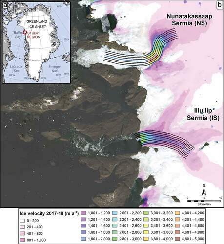
Figure 2. Frontal position relative to 9 April 1976 for (a), (b) Nunatakassaap Sermia (NS) and (c), (d) Illullip Sermia (IS). Terminus positions are color-coded according to date for (a) NS and (c) IS. NS’s terminus has remained attached to the pinning point at its northern margin (Point I, (a)). Gray boxes indicate the reference box used to calculate relative frontal positions. Base image source: Landsat 8, USGS Earth Explorer, 10 August 2020. Frontal positions are plotted over time and relative to 20 July 1976 for (b) NS and (d) IS. Note the differing y-axis scales for (b) and (d).

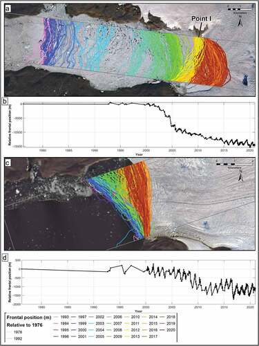
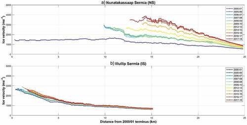
Figure 3. Interannual winter velocity changes at (a) Nunatakassaap Sermia (NS) and (b) Illullip Sermia (IS). Ice velocities are color-coded according to year of the winter velocity mosaic. Note that NS had a floating ice tongue in 2000–2001, which had collapsed by the subsequent winter velocity mosaic in 2005–2006. X-axis values are relative to the 2000–2001 termini for each glacier. Source: Joughin et al. (2010, 2015, updated 2018).

Here we used a range of remotely sensed data sets to assess changes in velocity, frontal position, and surface elevation at NS and IS for the period 2000 to 2020. Specifically, we assessed the patterns of velocity change at IS and NS using MEaSUREs data products to evaluate the impact of the ice tongue loss at NS and to identify differences in the seasonal velocity patterns between the two glaciers. We mapped the terminus positions of both glaciers from 2012 to 2020 using a combination of Landsat 8 and Sentinel-1 and -2 imagery to calculate annual retreat rates and integrated these data with earlier frontal positions from Carr, Vieli, and Stokes (2013). We then assessed the effect of retreat and acceleration on glacier thinning using the Arctic digital elevation model (DEM) and compared patterns of changes in glacier dynamics to the basal topography beneath each glacier. Finally, we calculated short-term (one- to four-week) calving rates and compared them to water depth and ice thickness to evaluate whether empirical calving relationships are applicable at these timescales and for these glaciers.

Methodology

Frontal position change

Frontal positions were mapped between April 2012 and December 2020 using the Google Earth Engine Digitization Tool, which allows users to manually digitize terminus positions online (Lea 2018). To obtain the best possible temporal coverage and resolve the seasonal cycle, Landsat 7 data were used for 2012 (available April–August), Landsat 8 for 2013–2014 (available March–October), and a combination of Landsat 8 and Sentinel-1 and -2 data from 2015–2020 (available January–December). For the period 2015–2020, we used a combination of Landsat 8 and Sentinel-2 data between March and October, when there was sufficient light to use visible imagery, and Sentinel-1 radar data for the winter months of January to February and October to December. For all image types, we only used imagery where the terminus was clearly visible and distinguishable from the ice melange, and for optical imagery where the terminus was not obscured by cloud. For the Landsat 7 and 8 data (spatial resolution 30 m) and Sentinel-2 (spatial resolution 10 m), we used true-color composite imagery; that is, red, green, blue composite. For Sentinel-1, we used Ground Range Detected Level 1 data, which has a spatial resolution of 10 m. The temporal coverage of the satellite imagery, and hence our frontal positions, is shown in Supplementary Figure 1. For the period 2015–2020, we had only one month where we had fewer than two images at IS (Supplementary Figure 1). At NS, we had four months with less than two images and two months with no images (Supplementary Figure 1). For 2012–2014, image availability is substantially lower, although at least one image was available for most months between March and October (Supplementary Figure 1). Thus, we are confident that our data resolve the seasonal cycle in frontal positions between 2015 and 2020 and so this is the primary focus of our seasonal analysis.

The box method was used to calculate terminus positions (Moon and Joughin 2008; Carr, Stokes, and Vieli 2017), because it accounts for spatially uneven terminus retreat, which occurs at both NS and IS. The newly digitized terminus positions were combined with those from Carr, Vieli, and Stokes (2013), which mapped terminus retreat at NS and IS from 9 April 1976 to 24 May 2012. A common reference box was used for both data sets to produce a consistent record from 1976 to the end of the study period in 2020. The error for the Carr, Vieli, and Stokes (2013) data set was 28.9 m and primarily resulted from manual digitizing errors (Carr, Vieli, and Stokes 2013). For all new frontal positions, image geolocation was checked prior to digitizing each terminus trace, by comparing features that should not move between consecutive images (e.g., rock ridges). Thus, for the new frontal positions (May 2012–December 2020), there were no errors in geolocation for the imagery at the pixel resolution. As such, the errors are due to manual digitization, and we assessed this by repeatedly digitizing the terminus of each glacier five times on the same image. We did this for a subsample of ten images for each image type (i.e., Landsat, Sentinel-1, and Sentinel-2), spread throughout the year and the study period. The resultant error was 29.7 m for Landsat 8, 24.3 m for Sentinel-2, and 41.6 m for Sentinel-1. We therefore give an average error of 32 m for our frontal position data.

Velocity change

Interannual changes in ice velocities were assessed using the MEaSUREs Greenland Ice Sheet Velocity Map from InSAR Data, Version 2 product (Joughin, Smith, Howat, and Scambos 2010; Joughin et al. 2015, updated 2018). This data set comprises Greenland winter velocity maps derived from interferometric synthetic aperture radar (InSAR; Joughin et al. 2010) observations. For this study, we used all available winter velocity maps. The 500-m resolution product was used for consistency between years, because the 200-m resolution product is only available from 2014–2015 onwards (Supplementary Table 1). MEaSUREs Selected Glacier Site Velocity Maps generated from the InSAR Version 4 data set were used to provide seasonal velocity data from 2009 to 2020 (Joughin, Smith, Howat, Scambos, and Moon 2010; Joughin et al. 2021). This data set was derived using image pairs from the German Aerospace Center’s twin satellites TerraSAR-X/TanDEM-X. These InSAR-derived velocity data were acquired from the W74.50 N and W74.95 N grid squares and have a spatial resolution of 100 m (Supplementary Table 1).

For both the interannual and seasonal data, ice surface velocities were extracted along a series of flow lines, which were created parallel to each glacier’s central flow line (Figure 1). First, a velocity center profile was created for each glacier by delineating the area of fast flow and then calculating the Euclidean distance from this boundary. The velocity centreline was then extracted from the points furthest away from the bounding contour, according to the Euclidean distance. We then created additional flow lines parallel to the center line, offset at 500-m intervals, with the outermost flowlines being located at the lateral edges of fast flow and the bounding box used to extract terminus positions at each glacier. Ice velocities were then extracted at 100-m intervals along all profiles and average values were calculated. This provided the cross-glacier mean velocity at 100-m intervals up-glacier, for each time interval, which corresponds to the cross-glacier terminus changes calculated using the box method.

To investigate potential seasonal variations in ice velocity changes, the data extracted from the MEaSUREs Selected Glacier Site Velocity Maps were split into seasons: winter (December, January, February), spring (March, April, May), summer (June, July, August), and autumn (September, October, November). Where the dates for an ice velocity map spanned two seasons, the map was assigned the season with the most number of days; for example, an ice velocity map with the dates 31 August to 10 September would be assigned to autumn. We also assessed the relationship between seasonal velocity variations, distance inland from the terminus, and glacier frontal position by extracting velocity data at the most retreated 2020 terminus for each glacier and then at 1-km intervals inland. Using the error fields provided with the interannual velocity data set, errors at both NS and IS were generally less than 3 percent or 40 m a⁻¹, and errors were thus small relative to the measured velocities (Supplementary Figure 2). Percentage errors showed limited variation with distance inland, and error values were highest for the oldest velocity data (i.e., winter 2000–2001) and lowest for 2017–2018. Errors in the seasonal velocity data at NS and IS were less than 1.5 percent, which equates to less than 20 m a⁻¹ at most locations (Supplementary Figures 3 and 4). Percentage errors at NS were lowest nearest the terminus (<0.5 percent) and increased from ~ 22 km inland to ~0.5 to 1.5 percent (Supplementary Figure 3), whereas at IS the pattern of velocity errors was spatially variable (Supplementary Figure 4).

Surface elevation change

To assess surface elevation change, we used 2-m DEM timestamped strips from Arctic DEM (https://www.pgc.umn.edu/guides/arcticdem/introduction-to-arcticdem/). The specific tiles used are given in Supplementary Table 1. Arctic DEM is generated from stereo pairs of high-resolution optical satellite imagery (WorldView-1 to -3), using the software package Surface Extraction with TIN-based Search-space Minimization (Noh and Howat 2015). The data are processed to 2-m resolution and have an absolute accuracy of ~4-m in the horizontal and vertical directions. Surface elevation data were extracted at the centreline sampling points used in the ice velocity data (Figure 1). Data were available for NS and IS for the period 2010 to 2017, and we utilized all tiles that overlapped with our centreline sample points (Supplementary Table 1).

Bed elevation

Bed elevation data were obtained from BedMachine Version 3 data (https://sites.uci.edu/morlighem/dataproducts/bedmachine-greenland/; Morlighem et al. 2017). The data were produced by assimilating both offshore bathymetric data and ice thickness measurements from radar surveys using a mass conservation approach. The data have a spatial resolution of 150 m (Morlighem et al. 2017). We sampled bed topography along the centreline of our reference box used to calculate the frontal positions. This was to facilitate direct comparison of bed elevation and frontal position data. For NS, fjord bathymetry are derived from airborne gravity observations, and those upstream of the grounding line are from radar-constrained mass conservation (Supplementary Figure 5). Based on the error estimates supplied with the data, vertical errors in elevation along the centreline of the frontal position reference box averaged 31.3 m and are 29.3 m in the area occupied by the glacier front during our study period. Vertical errors within the fjord averaged 21.3 m, compared to 41.5 m for those upstream of the grounding line (Supplementary Figure 5). Peak bed errors occur between 7 and 8 km from the upstream reference line, reaching up to 200 m in the area where data have been interpolated (Supplementary Figure 5). At IS, fjord bathymetry was derived from bathymetric data and the area upstream of the grounding line from mass conservation (Supplementary Figure 6). Vertical elevation errors within the frontal position reference box (32.1 m) and the area occupied by the terminus (29.9 m) were very similar to those observed at NS. Vertical elevation errors offshore of the grounding line were very low (~2 m) in comparison to an average of 58.9 m for the IS study area overlain by grounded ice.

Excess buoyancy

To assess whether the study glaciers were close to flotation, we calculated excess buoyancy $\mathit{Hb}$, which is the thickness of the ice front in excess of that which would be floating. Following Cuffey and Paterson (2010), excess buoyancy is calculated as

$\mathit{Hb}=\mathit{Hm}-\frac{\mathit{\rho w}}{\mathit{\rho i}}\mathit{Hw}$

where $\mathit{Hm}$ is the ice thickness at the terminus; $\mathit{Hw}$is the water depth; $\mathit{\rho w}$is the density of ocean water, set as 1,028 kg m⁻³; and $\mathit{\rho i}$ is the density of ice, set as 910 kg m⁻³. Excess buoyancy was calculated at the sample points used for the surface elevation change data (Figure 1). At each point, we extracted surface elevation from the Arctic DEM data and bed elevation from BedMachine v3. This was done for all Arctic DEM dates where data were available for more than 75 percent of the transect. Ice thickness $\left(\mathit{Hm}\right)$ was calculated by subtracting the bed elevation from the surface elevation. Water depth $\left(\mathit{Hw}\right)$ was determined from the bed data, so that the ocean surface is zero and the bed elevation is the water depth. Excess buoyancy of 50 m or less was used to determine when calving rates might increase, as the glacier approaches flotation, based on empirical values from Columbia Glacier (Meier and Reeh 1994).

Calving rate

We calculated calving rates for both glaciers using the seasonal ice velocity data and our frontal position data. Specifically, we selected the frontal position closest to the start and end of each seasonal velocity pair so that we could calculate the retreat rate (m d⁻¹) and the ice flow (m d⁻¹), with the difference between the two being the calving rate (Pelto and Warren 1991; Warren 1994). It should be noted that here the calving rate represents all ablation at the ice front—that is, ablation via calving and melting—because it is not possible to separate the two with the available data (Cuffey and Paterson 2010). To explore potential controls on calving, mean water depth $\left(\mathit{Hw}\right)$ and mean ice thickness at the terminus $\left(\mathit{Hm}\right)$ were calculated across all terminus traces to obtain width-averaged water depth and ice thickness. We then calculated the mean water depth and ice thickness for the start and end date for each velocity pair. Finally, we regressed calving rate against mean water depth and mean ice thickness.

Results

Interannual frontal position change

Nunatakassaap Sermia retreated by 2,488 ± 32 m between 24 May 2012 (the last date in Carr, Vieli, and Stoke 2013) and the last available image in 2020 (26 December 2020; Figure 2). This equates to a retreat rate of 328 m a⁻¹ (Figure 2). In the longer-term context, retreat rates post 2012 have been similar to those from ~2006 onwards and far less than peak rates of retreat observed at NS between 2001 and 2005, when its ice tongue collapsed. Post-2012 retreat at NS has been greatest in the center of NS’s terminus, whereas its lateral margins have remained connected to the fjord margins, meaning that the terminus shape is concave inland (Figure 2). Retreat rates at IS were much lower than those at NS, with the glacier retreating at 41 m a⁻¹ (310 ± 32 m total retreat) between 2 June 2012 and 26 December 2020. Whereas NS showed an overall retreat trend from 2001, the temporal pattern at IS was more variable: the frontal position showed limited net change until 2007 and then retreat between 2008 and 2010 (Figure 2). Subsequently, the glacier front underwent a small net readvance between 2011 and July 2016, followed by a substantial net retreat between 27 April 2016 and 24 October 2016 (Figure 2). Between October 2016 and the end of the study period, there was no net change in terminus position (Figure 2). Retreat at IS was spatially uneven, with the greatest recession occurring on the northern ice margin (Figure 2).

Between 2013 and 2020, terminus positions at NS underwent a broadly similar seasonal cycle (Figure 2). The front was usually most advanced in July each year, ranging between 5 and 20 July, except in 2019 when the maximum advance occurred on 16 June (Figure 2). The seasonal minimum frontal position was generally attained in October or November, with the earliest date being 7 October 2017, but occurred as late as 25 January 2020 (Figure 2). This minimum terminus position was usually maintained for two to three months, before the terminus began to seasonally readvance in January or February (Figure 2). During the study period, the largest seasonal retreat at NS occurred between 16 June 2019 and 25 January 2020, totaling 2,674 ± 32 m (Figure 2). During this event, the terminus stopped retreating in October, as in other years, but underwent another phase of net retreat between 2 December 2019 and 25 January 2020 (Figure 2). When compared to the longer-term record, seasonal terminus position variations between 2012 and 2020 were broadly comparable in magnitude to those in 2005 to 2007, substantially larger than those between 2008 and 2012, and smaller than the seasonal retreat of 2004, when NS was going through its major retreat phase (Figure 2).

At IS, terminus positions reached their seasonal maxima between late April (earliest date: 27 April 2016) and early July (latest date: 9 July 2018) between 2012 and 2020. As at NS, seasonal minima were reached sometime between October (earliest date: 9 October 2015) and December (latest date: 18 December 2017). In most years, seasonal terminus fluctuations followed a similar pattern and magnitude from 2000, when data were of sufficient temporal resolution to resolve seasonal changes, to 2020 (Figure 2). However, this was interrupted by a large retreat event between 27 April 2016 and 24 October 2016, when the terminus receded by 1,161 ± 32 m (Figure 2), and similar events between June and November 2008 (961 ±32 m) and June and October 2009 (896 ± 32 m; Figure 2).

Interannual velocity change

Ice velocities at NS increased substantially between winter 2000–2001 and 2017–2018, with peak velocities increased from 1,652 m a⁻¹ (2000–2001) to 3,857 m a⁻¹ (Figure 3). Velocity increases were greatest in the region up to 20 km inland of the 2000–2001 terminus and gradually reduced with distance inland (Figure 3). The spatial pattern of ice velocities on NS changed markedly between 2000–2001 and 2017–2018: in 2000–2001, ice velocities ranged from ~1,600 m a⁻¹ near the terminus to 545 m a⁻¹ at 25 km inland, and ice velocities showed limited variation over the ice tongue. For 2017–2018, the range in velocities was much greater, from ~3,800 m a⁻¹ near the terminus to 878 m a⁻¹ 25 km inland (Figure 3). Temporally, ice velocities at NS increased markedly along the entire centreline profile between 2000–2001 and 2005–2006, with the maximum increase occurring closest to the terminus (Figure 3). Ice velocities were broadly similar between 2005–2006 and 2009–2010 (Figure 3). Between 2012–2013 and 2015–2016, ice velocities increased substantially up to 20 km inland (Figure 3). There was a slight speed-up between 2015–2016 and 2016–2017, and then velocities were broadly similar between 2016–2017 and 2017–2018 (Figure 3).

Ice velocities at IS increased during the study period, but acceleration was much smaller than observed at NS, and the majority of the speed-up occurred by 2008–2009 (Figure 3). The largest changes in ice velocities occurred within ~5 km of the 2000–2001 terminus and reduced gradually with distance inland, and the spatial variability in velocity change was far smaller than at NS (Figure 3). Ice velocities at IS were lowest in 2000–2001, with values of 2,609 m a⁻¹ at the terminus (Figure 3). As such, IS was flowing at almost double the speed of NS at the start of the study period. Ice velocities at IS remained similar between the winters of 2000–2001 to 2007–2008: terminus velocities ranged between ~2,600 and 2,700 m a⁻¹, which was comparable to NS (Figure 3). IS accelerated between 2007–2008 and 2008–2009, reaching peak values of 2,893 m a⁻¹ at the terminus (Figure 3). Ice velocities along IS’s profile then remained at similar values for the remainder of the study period, whereas terminus velocities ranged between ~2,500 and 2,700 m a⁻¹. By the end of the study period, terminus velocities at NS (4,527 m a⁻¹) were 40 percent higher than those at IS (3,222 m a⁻¹).

Seasonal velocity change

We investigate the seasonal components of interannual velocity changes at NS and IS from 2009 to 2020 (Figures 4 and 5). At NS, the pattern of velocity change along the centreline profile is similar between seasons and dominated by the interannual trend (Figure 4). For all seasons, ice velocities increased between 2009 and 2018, decreased in 2019, and increased again by 2020 (Figure 4). The spatial pattern of velocity change mirrors interannual patterns, with the most velocity change occurring close to the terminus (Figure 4). The seasonal cycle of ice velocities at NS has evolved over time. In 2009–2011, velocities showed limited seasonal variation, and small peaks in velocity occurred close to NS’s terminus in late autumn 2012 (2,484 m a⁻¹; 22 November) and 2013 (2,526 m a⁻¹; 9 November). In contrast, a substantial seasonal velocity cycle was evident from 2014 to the end of the record, close to NS’s terminus, with the magnitude of seasonal velocity variations reducing markedly with distance inland (Figure 6). Ice velocities reached their seasonal peaks in winter, with peaks mostly occurring in February but also in November and December. Seasonal lows in velocity occurred in late May and early June and were almost 1,000 m a⁻¹ slower than seasonal peaks for the same time period (Figure 6). Thus, the amplitude of seasonal velocity variations at NS has increased markedly over time, with peaks in winter and lows in early summer.

Figure 4. Seasonal variations in ice velocities at Nunatakassaap Sermia (NS) for (a) spring, (b) summer, (c) autumn, and (d) winter. Ice velocities are color-coded according to date. X-axis values are relative to the 2000–2001 termini for each glacier. Source: Joughin et al. (2020; seasonal velocity data from 2009 to 2018).

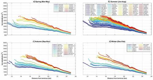
Figure 5. Seasonal variations in ice velocities at Illullip Sermia (IS) for (a) spring, (b) summer, (c) autumn, and (d) winter. Ice velocities are color-coded according to date. X-axis values are relative to the 2000–2001 termini for each glacier. Source: Joughin et al. (2020; seasonal velocity data from 2009 to 2018).

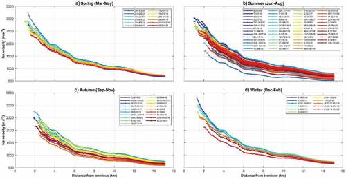
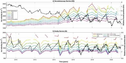
Figure 6. Seasonal velocity cycles between 2009 and 2020 for (a) Nunatakassaap Sermia (NS) and (b) Illullip Sermia (IS). For each glacier, data were sampled at the most retreated 2020 terminus and then at 1-km intervals inland for six intervals. This enabled the spatial pattern of seasonal velocity to be determined but accounted for terminus retreat. Velocity data are color-coded by distance inland and frontal position relative to 9 April 1976 is shown in black.

In contrast to NS, the pattern of velocity change at IS varied between seasons (Figure 5). Velocity changes were smallest in spring: the range in velocity was 875 m a⁻¹ at the terminus, with the lowest velocities occurring in 2020 and the highest in 2010 (Figure 5). Autumn velocities had a similar range (923 m a⁻¹) but reached their maximum in 2011 and minimum in 2018 (Figure 5). In autumn, velocities increased from 2009 to 2011, then decreased until 2018, before increasing again between 2018 and 2020 (Figure 5). The range in winter velocities was higher than spring or autumn (1,159 m a⁻¹). Maximum ice velocities were reached in 2009, after which velocities slowed to their minimum values in 2019 and increased slightly by 2020 (Figure 5). Changes in summer ice velocities at IS are complex and show considerable variability within and between years (Figure 5). Overall, the highest and lowest ice velocities occurred early in the study period (Figure 5). Overall, IS showed a net slowdown in spring and winter velocities, speed up, then slowdown in autumn, and high variability in the summer (Figure 5). In contrast to NS, we did not observe a net change in the seasonal cycle of ice velocities at IS during the study period (Figure 6). In most years we observed a mid-summer increase in seasonal velocities, which was followed by a seasonal low within one to three months (Figure 6). The magnitude of seasonal velocity variations reduced with distance inland, but the reduction was far less marked than at NS, and the difference between seasonal peaks and lows was smaller than at NS (maximum observed seasonal change = 899 m a⁻¹ in 2014; Figure 6). Thus, seasonal velocity changes at IS were smaller in magnitude than at NS and showed no clear trend over time but did propagate further inland (Figure 6). Seasonal peaks and lows in velocities at IS occurred during the summer, compared to winter peaks and early summer lows at NS.

Surface elevation change

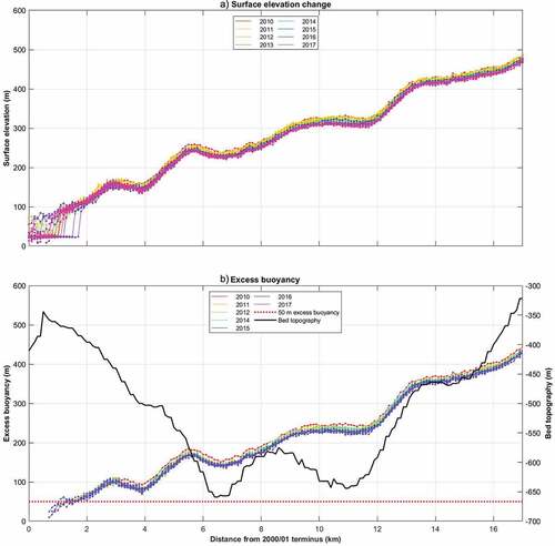
At NS, the ice surface thinned between 2010 and 2017 (Figure 7). Thinning was greatest between ~14.5 and 18.5 km upstream of the 2001–2001 terminus, where the glacier thinned by over 110 m between 2010 and 2017 (Figure 7). Proximal to the terminus and upstream of ~23.5 km from the terminus, there was ~30 m of thinning during the study period, whereas the section of the glacier between ~18.5 km and 23.5 km thinned by ~70 m (Figure 7). The highest rates of thinning occurred between 2012 and 2015 and were located between ~14.5 and 18.5 km upstream of the 2001–2001 terminus (Figure 7). At IS, we observe limited thinning between 2010 and 2017, with the surface lowering by ~20 m, and changes in elevation were relatively uniform along the centreline profile (Figure 8).

Figure 7. (a) Surface elevation changes at Nunatakassaap Sermia (NS) between 2010 and 2017. Elevation profiles are color-coded by year, and each year is composed of multiple profiles. Surface elevation data were extracted from Arctic digital elevation model (DEM) tiles along the glacier centreline and the x-axis distance is relative to the 2000–2001 glacier termini in the Joughin et al. (2010, 2015, updated 2018). (b) Excess buoyancy, calculated at the same sample points as in (a), using Arctic DEM tiles and bed topography from BedMachine v3 (black line). Transcripts are color-coded by date. Red line indicates where H_b equals 50 m, below which previous work suggests that calving rates will increase (Meier et al. 1994).

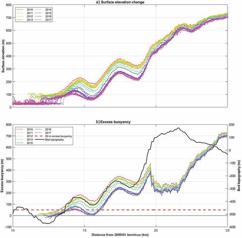
Figure 8. (a) Surface elevation changes at Illullip Sermia (IS) between 2010 and 2017. Elevation profiles are color-coded by year, and each year is composed of multiple profiles. Surface elevation data were extracted from Arctic digital elevation model (DEM) tiles along the glacier centreline and the x-axis distance is relative to the 2000–2001 glacier termini in the Joughin et al. (2010, 2015, updated 2018). (b) Excess buoyancy, calculated at the same sample points as in (a), using Arctic DEM tiles and bed topography from BedMachine v3 (black line). Transcripts are color-coded by date. Red line indicates where H_b equals 50 m, below which previous work suggests that calving rates will increase (Meier and Reeh 1994).

Basal topography, excess buoyancy and calving rates

Since 2012, NS has retreated down a reverse bedrock slope, with retreat being concentrated on the southern margin of its terminus (Figure 9). Its northern margin has remained on the bedrock ridge and at a comparatively narrow point within its fjord. This follows the rapid retreat of NS across an overdeepened section of its fjord between 2001 and 2005 and its temporary pause in retreat on a bedrock ridge in the late 2000s. The bed topography reaches a low just inland of the current terminus, before sloping upwards and increasing above sea level (Figure 9). At this point, the fjord widens considerably, and NS is no longer constrained within a fjord (Figure 9). NS’s excess buoyancy was 50 m or less (i.e., the glacier was close to flotation) over the lowest 1 to 2 km of the glacier for all years for which we have data (Figure 7). At the terminus, excess buoyancy values were negative for several years, indicating that the glacier was afloat (Figure 7). We observed no significant relationship between calving rate and either water depth or ice thickness at NS (Figure 10).

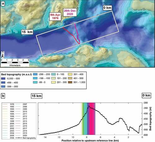
Figure 9. Basal topography of Nunatakassaap Sermia (NS). (a) Topography beneath NS and within its fjord, determined from BedMachine v3 (Morlighem et al. 2017). Contour interval is 200 m. White box indicates the extent of the reference box used to digitize terminus positions, and the terminus locations are marked for the earliest (9 April 1976; red) and latest (26 December 2020; pink) frontal positions available during the study period. (b) Location of NS’s terminus through time, relative to the upstream end of the reference box. Frontal positions are color-coded by year. Bed topography (black line) along the center of the reference box.

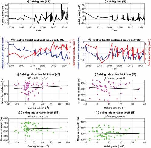
Figure 10. Calving rates and their relationship with potential controls for Nunatakassaap Sermia (NS) (left-hand panels) and Illullip Sermia (IS) (right-hand panels). Calving rates in meters per day (m d⁻¹) for (a) NS and (b) IS. Positive values indicate a net loss of ice via calving for a given time period (i.e., the rate of frontal retreat exceeds the forward ice velocity) and negative values indicate a net gain (i.e., the rate of frontal retreat is less than the forward ice velocity). Zero calving rate indicates that the rate of frontal retreat exactly balances the forward ice velocity. (c), (d) Relative frontal position (kilometers, relative to 9 April 1976) and terminus ice velocities in meters per day, to provide context for the calving rates. Calving rate regressed against mean ice thickness across the terminus at the time the calving rate was calculated, for (e) NS and (f) IS. The regression line is plotted in black and the R² and p values for the regression are displayed above the plot. (g), (h) Same as (e) and (f) but for mean water depth at the terminus.

Between 2012 and 2018, IS’s frontal position oscillated on the upglacier edge of a bedrock ridge, with most retreat occurring on its northern margin (Figure 11). IS’s terminus has occupied this basal topographic ridge since at least 1976, although it has gradually retreated back across it (Figure 11). The ridge also represents a comparatively narrow point in the fjord. Inland of the 2018 terminus position, the bed topography deepens and widens considerably. Excess buoyancy at IS was generally above 50 m, meaning that the glacier was not usually close to flotation. Values less than 50 m were observed on individual transects in 2011, 2016, and 2017, but these extended only 400 m inland (Figure 8). As at NS, there was no significant relationship between calving rate and either water depth or ice thickness at IS, and peak calving rates were lower than at NS.

Figure 11. Basal topography of Illullip Sermia (IS). (a) Topography beneath IS and within its fjord, determined from BedMachine v3 (Morlighem et al. 2017). Contour interval is 100 m. White box indicates the extent of the reference box used to digitize terminus positions, and the terminus locations are marked for the earliest (9 April 1976; red) and latest (22 September 2018; pink) frontal positions available during the study period. (b) Location of IS’s terminus through time, relative to the upstream end of the reference box. Frontal positions are color-coded by year. Bed topography (black line) along the center of the reference box.

Discussion

Interannual patterns in ice dynamics

At NS, net retreat rates remained relatively constant, at ~310 m a⁻¹, following the collapse of its ice tongue in 2005 (Figure 2). These retreat rates are high in comparison to elsewhere in northwest Greenland, and Greenland more broadly (Carr, Stokes, and Vieli 2017), and exceed rates observed after the loss of major sections of large ice tongues in northern Greenland (Hill, Carr et al. 2018) and at SK (Joughin et al. 2008, 2012, 2020). Major periods of retreat at NS occurred outside of its usual seasonal period of retreat (i.e., July to October/November) and are characterized by retreat persisting later into the year and limited seasonal advance (Figures 2 and 6). For example, in 2019, 2006, and 2005, retreat continued until January of the following year and seasonal readvance was very limited (Figures 2 and 6). Thus, major retreats at NS occurred during the winter and resulted from both higher rates of retreat and elongation of the seasonal retreat period.

Ice velocities at NS increased markedly after the collapse of its tongue, from a maximum of 1,791 m a⁻¹ (2000–2001) to 4,527 m a⁻¹ (2017–2018; Figures 2 and 3). This doubling of speed is comparable to changes observed at SK (e.g., Joughin, Abdalati, and Fahnestock 2004; Joughin et al. 2014, 2020) and Zachariae Isstrøm (Mouginot et al. 2015; Hill, Carr et al. 2018) following the disintegration of their ice tongues. However, it contrasts with the limited acceleration observed on many northern Greenland glaciers following major calving events from their ice tongues; for example, C. H. Ostenfeld Gletsjer, Petermann Gletsjer, Steensby and Hagen Brae (Hill, Carr et al. 2018). This difference in dynamic response to ice tongue loss is likely because the tongues at NS, Zachariae Isstrøm, and SK provide substantial resistance to flow and those elsewhere providing limited resistance, due to their weak and/or fractured state (Hill, Carr, and Stokes 2017; Hill, Carr et al. 2018; Hill, Gudmundsson et al. 2018). The spatial pattern of changes in surface elevation and velocity at NS supports this hypothesis: NS thinned substantially within ~20 km of the terminus (Figure 7) and ice acceleration was greatest closest to the front after retreat (Figure 3), suggesting that loss of resistive stress may have facilitated drawdown of inland ice and acceleration.

The (non-mutually exclusive) processes that can drive Greenland outlet glacier acceleration (Catania et al. 2020) are (1) enhanced basal lubrication of the glacier, via summer meltwater inputs; (2) terminus retreat causing inland acceleration, due to loss of downstream resistive stress (Howat et al. 2005; Amundson et al. 2008); (3) glacier thinning causing a reduction in effective pressure and thus increased sliding speed (Bindschadler 1983; Meier and Post 1987; Pfeffer, Harper, and O’Neel 2008); and (4) thinning caused by processes 2 and 3 steepens the glacier slope, causing ice acceleration to diffuse further up glacier (Payne et al. 2004; Howat, Joughin, and Scambos 2007; Joughin et al. 2008). We suggest that process 1 plays a limited role in the acceleration observed at NS, because our data show that velocity increases were comparable in magnitude between each season of the year (Figure 4), whereas acceleration due to meltwater should show strong seasonality (Moon et al. 2014). Instead, we suggest that ice acceleration was initially triggered by the loss of buttressing from NS’s ice tongue (process 2) and continued acceleration was facilitated by indirect responses to this loss—that is, processes 3 and 4—as observed at SK (Joughin et al. 2012). This is supported by the strong increase in ice velocities during NS’s ice tongue breakup (2001–2005) and by the thinning and steepening of the surface slope observed at NS during the study period (Figure 7), as per processes 3 and 4. Thus, our data suggest that ice tongue loss and subsequent feedbacks can explain the majority of the observed acceleration at NS.

In contrast to the sustained retreat at NS, retreat rates at IS were much lower and variable over the study period: the glacier retreated by only 1,085 ± 32 m between 1976 and 2020 (Figure 2), and the terminus underwent net retreat in certain years (e.g., 2008, 2009, and 2016) and net advance in others (e.g., 2011–2016). Contrary to NS, the periods of net retreat in 2008, 2009, and 2016 occurred during the usual seasonal retreat period; that is, between April and November (Figures 2 and 6). This suggests that IS retreated due to an increased rate of ice loss, rather than an extension of the seasonal period of retreat, and this retreat occurred largely during spring, summer, and early autumn (i.e., the warm period of the year). Changes in interannual velocities at IS were also far smaller in magnitude than at NS, although we did observe increasing interannual ice velocities between 2007–2008 and 2009–2010, which coincides with terminus retreat (Figures 2 and 3). We observed limited inland thinning, and ice velocity changes are largely confined to within ~5 km of the terminus (Figure 3). Thus, we suggest that small variations in resistive stresses, caused by comparatively small fluctuations in terminus position (process 2), may have some impact on ice velocities, but subsequent feedbacks and indirect effects of these changes in resistive stress (processes 3 and 4) are limited, unlike at NS.

Seasonal patterns in ice dynamics

Nunatakassaap Sermia

Data availability enable us to resolve the seasonal cycle of frontal positions from 2014 onwards. During this period, NS’s seasonal range in terminus position was ~1-2 ± 32 km, which is comparable to SK during the 2010s (Joughin et al. 2020). Except for winter 2016, the timing of the seasonal frontal position cycle was similar between years, with the front usually reaching its most advanced point in July and its minimum in October or November, before recommencing its seasonal advance in January or February (Figures 2 and 6). Seasonal velocities were out of phase with terminus position, so that velocities increased during periods of seasonal terminus retreat and peak speeds occurred when the terminus was near its seasonally most retreated point (Figure 6). Conversely, speeds reduced during seasonal retreat and seasonal lows in velocity occurred in late May to early June, shortly before the terminus reached its maximum extent in early to mid-July (Figure 6).

Following the classification of seasonal ice velocity behavior by Moon et al. (2014), we suggest that NS exhibits aspects of both type 1 (i.e., sensitive to terminus position) and type 3 (i.e., sensitive to meltwater) behavior but does not fit fully into either category. NS matches type 1 behavior, because it retains high speeds over winter and early spring, and seasonal velocity variations correspond to terminus positions (Figure 6; Moon et al. 2014; Vijay et al. 2019). However, NS decelerates from late spring to early summer and reaches its velocity minima in July (Figure 6), whereas type 1 glaciers usually accelerate during this period (Moon et al. 2014; Vijay et al. 2019). At type 3 glaciers, velocities reach a minima in late summer, due to the switch from inefficient to efficient subglacial drainage (Moon et al. 2014; Vijay et al. 2019). This corresponds with NS’s July velocity minima but does not fit with continued acceleration during the winter months, when meltwater should be scarce, and the lack of velocity peaks in the early melt season, when the subglacial drainage system should be inefficient in type 3 glaciers. (Figure 6; Moon et al. 2014; Vijay et al. 2019). Thus, NS’s seasonal behavior does not fit within a single category, but its interannual and seasonal patterns of behavior suggest that variations in terminus position impact its flow speed and that the role of meltwater is likely to be limited.

At NS, the magnitude of seasonal cycles in frontal position and ice velocity evolved during the study period (Figures 2 and 6). After its major retreat phase (2001–2005), NS underwent comparatively large seasonal retreats in 2006 (1,581 ± 32 m) and 2007 (1,172 ± 32 m; Figure 6). Seasonal variations were then relatively limited between 2008 and 2013, before increasing again between 2014 and the end of the study period in 2020, with the maximum seasonal retreat being 2,733 ± 32 m in 2019 (Figures 2 and 6). Higher magnitude seasonal frontal position variations from 2014 onwards coincided with larger seasonal velocity fluctuations, supporting the idea that terminus position is the primary control on ice velocities at NS.

Illullip Sermia

At IS, we can resolve seasonal frontal position cycles from 2000 onwards (Figures 2 and 6). During this period, the magnitude of seasonal frontal position variations was generally 500 to 600 ± 32 m, which was considerably smaller than the range observed at NS (Figures 2 and 6). The timing of these seasonal cycles was more variable than at NS, with the seasonal maxima ranging between late April and early July and the seasonal minima occurring between early October and mid-December (Figure 6). Unlike at NS, seasonal ice velocities at IS were in-phase with frontal position, so that seasonal velocities peaked in mid-summer and coincided with the maximum seasonal frontal position (Figure 6). Ice velocities then reduced rapidly over the following approximately two months, coincident with terminus retreat (Figure 6). Ice velocities reached their seasonal minima in late August to early September, whereas terminus position minima occurred between October and December (Figure 6). Thus, IS most closely matches type 2 glaciers, which have a strong summer speed-up and then deceleration after mid-summer (Moon et al. 2014). Type 2 glaciers are thought to respond to seasonal variations in meltwater inputs, with early summer speed-up corresponding to seasonally high meltwater inputs (Moon et al. 2014). Thus, we suggest that IS’s seasonal velocity variations are primarily influenced by runoff, as opposed to variations in frontal position (Figure 6).

Impact of glacier-specific factors on ice dynamics

We attribute the observed differences in retreat patterns between the two glaciers to their basal topography (Figures 2, 9, and 10). Retreat from 2012 onwards has brought NS’s terminus into both a deeper and wider section of the fjord (Figures 2 and 9). This may have facilitated the high observed retreat rates via buoyancy driven feedbacks, as the glacier retreated into deeper water (e.g., Meier and Post 1987; Schoof 2007; Schoof, Davis, and Popa 2017; Catania et al. 2018, 2020), and via the reduction in lateral resistive stresses, as the fjord widened (Warren and Glasser 1992; Raymond 1996; Jamieson et al. 2012). Notably, NS’s terminus has remained attached to the pinning point at its northern margin (Figure 2; Point I), whereas the southern portion has retreated into a wider and deeper section of the fjord, which explains the uneven retreat of NS’s terminus from 2012 onwards. In contrast, IS has remained on the bedrock ridge it has occupied since at least 1976 and thus has not experienced a wider or deeper fjord (Figures 2 and 10). Thus, differences in both the depth and width of the underlying topography may account for the different retreat rates NS and IS, as observed elsewhere in Greenland (e.g., Porter et al. 2014; Carr et al. 2015; Bartholomaus et al. 2016; Bunce et al. 2018; Catania et al. 2018). Numerical modeling work should be conducted to determine how both glaciers will evolve in the future, as the basal troughs of both glaciers widen considerably inland of their current terminus positions and IS is backed by a large basal overdeepening (Figures 9 and 10). Furthermore, additional data on fjord bathymetry and basal topography proximal to the sills of both NS and IS are needed, to further constrain their impacts on ice dynamics, because uncertainties in bedrock geometry are comparatively high in this area (Supplementary Figures 5 and 6).

Available data suggest that NS was close to flotation for at least 1 to 2 km inland for all dates for which Arctic DEM data were available (2010–2017; Figure 7). In contrast, IS was close to flotation only for a small number of dates and only up to 400 m inland (Figure 8). Notwithstanding errors in the basal topography data and the Arctic DEM coverage, the available evidence suggests that NS’s terminus was consistently close to flotation between 2010 and 2017, whereas IS’s was only close to flotation occasionally and over a limited area. We suggest that this likely contributed to the patterns in dynamics observed at NS and IS. Interestingly, our data show no significant correlation between calving velocities and either water depth or ice thickness at the terminus for either glacier at weekly to monthly timescales (Figure 10). We suggest that this lack of apparent relationship may be due to the comparatively high temporal resolution of our data compared to previous studies (e.g., Brown et al. 1983; Pelto and Warren 1991) that have determined empirical relationships and highlights the potential pitfalls of using empirical calving relationships at short timescales.

After the ice tongue collapse NS, ice velocities showed limited change between winter 2005–2006 and 2009–2010 (Figure 3) and seasonal frontal position variations were comparatively small (Figure 2), which coincided with the terminus retreating onto a sill and a narrower section of the fjord (Figure 9). These changes would have reduced the grounding line thickness at NS, which in turn would reduce its discharge and therefore ice velocities (e.g., Schoof 2007; Joughin and Alley 2011; Schoof, Davis, and Popa 2017; Catania et al. 2018). The narrowing fjord would have increased lateral resistive stress and cause the terminus to thicken due to conservation of mass (Echelmeyer et al. 1994; Raymond 1996), further reducing retreat. Taken together, this would explain the observed reduction in ice velocities between winter 2005–2006 and 2009–2010 (Figure 3).

In 2010, NS’s terminus retreated from its bedrock ridge and onto a reverse bed slope, although its terminus remained on a pinning point at its northern margin (Figures 2 and 9). The terminus retreated into deeper water and approached flotation near its terminus (Figures 7 and 9), which would reverse the feedbacks outlined above: thicker ice at the grounding line promotes higher ice velocities, higher calving rates, and increased ice discharge, whereas a terminus near flotation is more vulnerable to fracture and increased calving rates (e.g., van der Veen 1996, 1998; Pfeffer 2007; Schoof 2007; Amundson et al. 2010; Joughin and Alley 2011; Vieli and Nick 2011). This is reflected in our interannual velocity data, which show that NS accelerated between winter 2009–2010 and 2015–2016 (Figure 3). Thus, we suggest that interannual patterns of ice velocity change at NS were initially triggered by the loss of its ice tongue (process 2) and continued by a series of feedbacks (processes 3 and 4) but were also modulated by NS’s basal topography. In contrast, interannual changes in frontal position and ice velocity were limited at IS, because it remained on its bedrock ridge throughout the study period (Figure 11) and it approached flotation only over a limited area and time interval (Figure 8). As such, IS’s bedrock topography enabled limited change, as observed elsewhere in Greenland (e.g., Enderlin, Howat, and Vieli 2013; Carr et al. 2015; Catania et al. 2018, 2020). Overall, our results highlight the importance of considering bedrock topography in relation not just to initial retreat but also to the longer-term evolution of the glacier after the retreat event.

Conclusions

Following the collapse of its ice tongue in 2005, retreat rates at NS far exceeded those at IS and the Greenland-wide average. After the ice tongue collapse, ice velocities at NS doubled, and it thinned substantially within ~20 km of the ice front. Thus, we suggest that acceleration and thinning were initially triggered by reduced buttressing, due to the loss of the ice tongue, and were then sustained by subsequent feedbacks between glacier thinning, surface slope, and effective pressure, as NS retreated into a deeper and wider fjord. In contrast, interannual velocity changes were much smaller at IS and confined to within ~5 km of the terminus, suggesting that observed velocity changes may reflect small changes in resistive stress due to terminus fluctuations but that the feedbacks seen at NS do not develop, likely due to the location of IS’s terminus on a bedrock ridge. This is supported by NS being close to flotation with ~1 to 2 km of its terminus throughout the study period, whereas flotation at IS was spatially limited and occasional.

The timing of seasonal retreats differed between NS and IS: at NS, episodes of substantial net retreat occurred due to seasonal retreat persisting through the winter and winter readvance being limited. In contrast, net retreat at IS occurred via higher retreat rates during the late spring, summer, and early autumn. We also observed major differences in the relative timings of seasonal variations in frontal position and ice velocities at the two glaciers. At NS, seasonal velocities were out of phase with terminus position, so that peak speeds coincided with the most seasonally retreat frontal position and velocities increased during seasonal terminus retreat. In contrast, seasonal velocities and frontal positions co-varied at IS, so that ice velocities were lost when the terminus was most retreat and terminus retreat was associated with reduce velocities. Our data suggest that seasonal ice velocities are controlled by terminus position at NS and by meltwater at IS, although NS’s behavior does not fit within a single seasonal velocity category. We observed no significant correlation between calving rates and either water depth or terminus thickness within our seasonal data, suggesting that empirical relationships may not hold at weekly to monthly timescales. Despite the spatial proximity of NS and IS, our results demonstrated marked differences in (1) the timing of seasonal cycles in frontal position and ice velocity and the relationship between them, (2) the likely drivers of seasonal velocity cycles, (3) the seasonal timing of episodes of substantial net retreat, and (4) the dynamic response to interannual retreat. This demonstrates that glacier-specific factors can strongly modulate the dynamics of Greenland outlet glaciers at seasonal to decadal timescales.

Disclosure statement

No potential conflict of interest was reported by the author(s).

Supplementary material

Supplemental data for this article can be accessed online at https://doi.org/10.1080/15230430.2023.2186456.

Additional information

Funding

This work was supported by the Natural Environment Research Council via a IAPETUS2 PhD studentship awarded to E. Carr.

References

- Amundson, J. M., and J. Burton. 2018. Quasi‐static granular flow of ice mélange. Journal of Geophysical Research: Earth Surface 123 (9):2243–22. doi:10.1029/2018JF004685.
- Amundson, J. M., M. Fahnestock, M. Truffer, J. Brown, M. P. Lüthi, and R. J. Motyka. 2010. Ice mélange dynamics and implications for terminus stability, Jakobshavn Isbræ, Greenland. Journal of Geophysical Research 115 (F0):1005. doi:10.1029/2009JF001405.
- Amundson, J. M., M. Fahnestock, M. Truffer, V. Tsai, and M. West, 2008: Analysis of seismic waveforms generated during iceberg calving events, Jakobshavn Isbræ, Greenland. American Geophysical Union, Fall Meeting. San Francisco, CA, USA. Abstract #C22A-02.
- Andersen, M. L., L. Stenseng, H. Skourup, W. Colgan, S. A. Khan, S. S. Kristensen, S. B. Andersen, J. E. Box, A. P. Ahlstrøm, and X. Fettweis. 2015. Basin-scale partitioning of Greenland ice sheet mass balance components (2007–2011). Earth and Planetary Science Letters 40:989–95.
- Bartholomaus, T. C., L. A. Stearns, D. A. Sutherland, E. L. Shroyer, J. D. Nash, R. T. Walker, G. Catania, D. Felikson, D. Carroll, M. J. Fried, et al. 2016. Contrasts in the response of adjacent fjords and glaciers to ice-sheet surface melt in West Greenland. Annals of Glaciology 57 (73):25–38. doi:10.1017/aog.2016.19.
- Benn, D. I., C. R. Warren, and R. H. Mottram. 2007. Calving processes and the dynamics of calving glaciers. Earth Science Reviews 82 (3–4):143–79.
- Bindschadler, R. 1983. The importance of pressurized subglacial water in separation and sliding at the glacier bed. Journal of Glaciology 29 (101):3–19. doi:10.1017/S0022143000005104.
- Box, J. E. 2013. Greenland ice sheet mass balance reconstruction. Part II: Surface mass balance (1840–2010). Journal of Climate 26 (18):6974–89. doi:10.1175/JCLI-D-12-00518.1.
- Box, J. E., M. Sharp, G. Aðalgeirsdóttir, M. Ananicheva, M. L. Andersen, J. R. Carr, C. Clason, W. Colgan, L. Copland, A. F. Glazovsky, et al. 2017. Changes to Arctic land ice. In Snow, Water, Ice and Permafrost in the Arctic (SWIPA) 2017, ed. J. E. Box and M. Sharp, 137–68. Oslo, Norway: Arctic Monitoring and Assessment Programme (AMAP).
- Brown, C., W. Sikonia, A. Post, L. Rasmussen, and M. Meier. 1983. Two calving laws for grounded iceberg-calving glaciers. Annals of Glaciology 4:295–295. doi:10.3189/S0260305500005644.
- Bunce, C., J. R. Carr, P. W. Nienow, N. Ross, and R. Killick. 2018. Ice front change of marine-terminating outlet glaciers in northwest and southeast Greenland during the 21st century. Journal of Glaciology 64 (246):523–35. doi:10.1017/jog.2018.44.
- Carr, J. R., C. R. Stokes, and A. Vieli. 2013. Recent progress in understanding marine-terminating Arctic outlet glacier response to climatic and oceanic forcing: Twenty years of rapid change. Progress in Physical Geography 37 (4):435–66.
- Carr, J. R., C. R. Stokes, and A. Vieli. 2017. Threefold increase in marine-terminating outlet glacier retreat rates across the Atlantic Arctic: 1992–2010. Annals of Glaciology 58 (74):72–91. doi:10.1017/aog.2017.3.
- Carr, J. R., A. Vieli, and C. R. Stokes. 2013. Climatic, oceanic and topographic controls on marine-terminating outlet glacier behavior in north-west Greenland at seasonal to interannual timescales. Journal of Geophysical Research 118 (3):1210–26. doi:10.1002/jgrf.20088.
- Carr, J. R., A. Vieli, C. Stokes, S. Jamieson, S. Palmer, P. Christoffersen, J. Dowdeswell, F. Nick, D. Blankenship, and D. Young. 2015. Basal topographic controls on rapid retreat of Humboldt Glacier, northern Greenland. Journal of Glaciology 61 (225):137–50. doi:10.3189/2015JoG14J128.
- Catania, G., L. Stearns, T. Moon, E. Enderlin, and R. Jackson. 2020. Future evolution of Greenland’s marine‐terminating outlet glaciers. Journal of Geophysical Research: Earth Surface 125 (2). doi:10.1029/2019JF005206.
- Catania, G., L. Stearns, D. Sutherland, M. Fried, T. Bartholomaus, M. Morlighem, E. Shroyer, and J. Nash. 2018. Geometric controls on tidewater glacier retreat in central western Greenland. Journal of Geophysical Research: Earth Surface 123 (8):2024–38. doi:10.1029/2017JF004499.
- Cuffey, K. M., and W. S. B. Paterson. 2010. The physics of glaciers. Burlington, MA: Elsevier.
- Echelmeyer, K. A., W. D. Harrison, C. Larsen, and J. E. Mitchell. 1994. The role of the margins in the dynamics of an active ice stream. Journal of Glaciology 40 (136):527–38. doi:10.1017/S0022143000012417.
- Enderlin, E. M., and I. M. Howat. 2013. Submarine melt rate estimates for floating termini of Greenland outlet glaciers (2000–2010). Journal of Glaciology 59 (213):67–75. doi:10.3189/2013JoG12J049.
- Enderlin, E. M., I. M. Howat, S. Jeong, M.-J. Noh, J. H. van Angelen, and M. R. van den Broeke. 2014. An improved mass budget for the Greenland ice sheet. Geophysical Research Letters 41 (3):2013GL059010. doi:10.1002/2013GL059010.
- Enderlin, E. M., I. M. Howat, and A. Vieli. 2013. High sensitivity of tidewater outlet glacier dynamics to shape. The Cryosphere 7 (3):1007–15. doi:10.5194/tc-7-1007-2013.
- Fettweis, X., B. Franco, M. Tedesco, J. van Angelen, J. M. V. D. B. Lenaerts, and H. Gallée. 2013. Estimating the Greenland ice sheet surface mass balance contribution to future sea level rise using the regional atmospheric climate model MAR. The Cryosphere 7 (2):469–89. doi:10.5194/tc-7-469-2013.
- Gudmundsson, G. H., J. Krug, G. Durand, L. Favier, and O. Gagliardini. 2012. The stability of grounding lines on retrograde slopes. The Cryosphere 6 (6):1497–505. doi:10.5194/tc-6-1497-2012.
- Higgins, A. K. 1988. Glacier velocities in North and North-East Greenland. Grønlands Geologiske Undersogelse Rapport 140:102–05. doi:10.34194/rapggu.v140.8046.
- Higgins, A. K. 1990. North Greenland glacier velocities and calf ice production. Polarforschung 60 (1):1–23.
- Hill, E. A., R. J. Carr, and C. R. Stokes. 2017. A review of recent changes in major marine-terminating outlet glaciers in northern Greenland. Frontiers in Earth Science 4. doi:10.3389/feart.2016.00111.
- Hill, E. A., J. R. Carr, C. R. Stokes, and G. H. Gudmundsson. 2018. Dynamic changes in outlet glaciers in northern Greenland from 1948 to 2015. The Cryosphere 12 (10):3243–63. doi:10.5194/tc-12-3243-2018.
- Hill, E. A., G. H. Gudmundsson, J. R. Carr, and C. R. Stokes. 2018. Velocity response of Petermann Glacier, northwest Greenland, to past and future calving events. The Cryosphere 12 (12):3907–21. doi:10.5194/tc-12-3907-2018.
- Hill, E. A., G. H. Gudmundsson, J. R. Carr, and C. R. Stokes. 2021. Twenty-first century response of Petermann Glacier, northwest Greenland to ice shelf loss. Journal of Glaciology 67 (261):147–57. doi:10.1017/jog.2020.97.
- Holland, D. M., R. H. D. Y. B. Thomas, M. H. Ribergaard, and B. Lyberth. 2008. Acceleration of Jakobshavn Isbræ triggered by warm subsurface ocean waters. Nature Geoscience 1:659–664. doi:10.1038/ngeo316.
- Howat, I. M., and A. Eddy. 2011. Multi-decadal retreat of Greenland’s marine-terminating glaciers. Journal of Glaciology 57 (203):389–96. doi:10.3189/002214311796905631.
- Howat, I. M., I. Joughin, M. Fahnestock, B. E. Smith, and T. Scambos. 2008. Synchronous retreat and acceleration of southeast Greenland outlet glaciers 2000-2006; Ice dynamics and coupling to climate. Journal of Glaciology 54 (187):1–14. doi:10.3189/002214308786570908.
- Howat, I. M., I. Joughin, and T. A. Scambos. 2007. Rapid changes in ice discharge from Greenland outlet glaciers. Science 315 (5818):1559–61. doi:10.1126/science.1138478.
- Howat, I. M., I. Joughin, S. Tulaczyk, and S. P. Gogineni. 2005. Rapid retreat and acceleration of Helheim Glacier, east Greenland. Geophysical Research Letters 32 (22). Retrieved from https://escholarship.org/uc/item/5gp0z2kx
- The IMBIE Team. 2020. Mass balance of the Greenland Ice Sheet from 1992 to 2018. Nature 579(7798):233–39. doi:10.1038/s41586-019-1855-2.
- Jamieson, S. S. R., A. Vieli, S. J. Livingstone, C. Ó Cofaigh, C. R. Stokes, C.-D. Hillenbrand, and J. Dowdeswell. 2012. Ice stream stability on a reverse bed slope. Nature Geoscience 5 (11):799–802. doi:10.1038/ngeo1600.
- Johnson, H. L., A. Münchow, K. K. Falkner, and H. Melling. 2011. Ocean circulation and properties in Petermann Fjord, Greenland. Journal of Geophysical Research 116 (C1). doi:10.1029/2010JC006519.
- Joughin, I., W. Abdalati, and M. Fahnestock. 2004. Large fluctuations in speed on Greenland’s Jakobshavn Isbræ glacier. Nature 432 (2):608–10. doi:10.1038/nature03130.
- Joughin, I., and R. B. Alley. 2011. Stability of the West Antarctic ice sheet in a warming world. Nature Geoscience 4:506–13. doi:10.1038/ngeo1194.
- Joughin, I., I. M. Howat, M. Fahnestock, B. Smith, W. Krabill, R. B. Alley, H. Stern, and M. Truffer. 2008. Continued evolution of Jakobshavn Isbrae following its rapid speedup. Journal of Geophysical Research 113 (F4). doi:10.1029/2008JF001023.
- Joughin, I., I. Howat, B. Smith, and T. Scambos. 2021. MEaSUREs greenland ice velocity: Selected glacier site velocity maps from InSAR, version 4 [data set]. NASA National Snow and Ice Data Center Distributed Active Archive Center, Boulder, Colorado, USA. https://nsidc.org/data/nsidc-0481/versions/4
- Joughin, I., D. E. Shean, B. E. Smith, and D. Floricioiu. 2020. A decade of variability on Jakobshavn Isbræ: Ocean temperatures pace speed through influence on mélange rigidity. The Cryosphere 14 (1):211. doi:10.5194/tc-14-211-2020.
- Joughin, I., B. E. Smith, I. M. Howat, D. Floricioiu, R. B. Alley, M. Truffer, and M. Fahnestock. 2012. Seasonal to decadal scale variations in the surface velocity of Jakobshavn Isbrae, Greenland: Observation and model-based analysis. Journal of Geophysical Research 117 (F2). doi:10.1029/2011JF002110.
- Joughin, I., B. E. Smith, I. Howat, and T. Scambos. 2010. MEaSUREs Greenland ice sheet velocity map from InSAR data. Boulder, CO: National Snow and Ice Data Center. Digital media.
- Joughin, I., B. Smith, I. Howat, and T. Scambos. 2015. MEaSures Greenland ice sheet velocity map from InSAR data, Version 2, updated 2018. Boulder, CO: NASA National Snow and Ice Data Center Distributed Active Archive Center. doi:10.5067/OC7B04ZM9G6Q.
- Joughin, I., B. Smith, I. M. Howat, T. Scambos, and T. Moon. 2010. Greenland flow variability from ice-sheet-wide velocity mapping. Journal of Glaciology 56 (197):415–30. doi:10.3189/002214310792447734.
- Joughin, I., B. Smith, D. Shean, and D. Floricioiu. 2014. Brief communication: Further summer speedup of Jakobshavn Isbræ. The Cryosphere 98:209–14. doi:10.5194/tc-8-209-2014.
- Khan, S. A., J. Wahr, M. Bevis, I. Velicogna, and E. Kendrick. 2010. Spread of ice mass loss into northwest Greenland observed by GRACE and GPS. Geophysical Research Letters 37 (6). doi:10.1029/2010GL042460.
- Khazendar, A., I. G. Fenty, D. Carroll, A. Gardner, C. M. Lee, I. Fukumori, O. Wang, H. Zhang, H. Seroussi, and D. Moller. 2019. Interruption of two decades of Jakobshavn Isbrae acceleration and thinning as regional ocean cools. Nature Geoscience 12 (4):277–83. doi:10.1038/s41561-019-0329-3.
- Kneib-Walter, A., M. P. Lüthi, M. Funk, G. Jouvet, and A. Vieli. 2022. Observational constraints on the sensitivity of two calving glaciers to external forcings. Journal of Glaciology 1–16. doi:10.1017/jog.2022.74.
- Kneib-Walter, A., M. P. Lüthi, L. Moreau, and A. Vieli. 2021. Drivers of recurring seasonal cycle of glacier calving styles and patterns. Frontiers in Earth Science 9:667717. doi:10.3389/feart.2021.667717.
- Lea, J. M. 2018. The Google Earth Engine Digitisation Tool (GEEDiT) and the Margin change Quantification Tool (MaQiT) – Simple tools for the rapid mapping and quantification of changing earth surface margins. Earth Surface Dynamics 6 (3):551–61. doi:10.5194/esurf-6-551-2018.
- McFadden, E. M., I. M. Howat, I. Joughin, B. Smith, and Y. Ahn. 2011. Changes in the dynamics of marine terminating outlet glaciers in west Greenland (2000–2009). Journal of Geophysical Research 116 (F2). doi:10.1029/2010JF001757.
- Meier, M. F., and A. Post. 1987. Fast tidewater glaciers. Journal of Geophysical Research 92 (B9):9051–58 doi:10.1029/JB092iB09p09051.
- Meier, M. F., and N. Reeh. 1994. Columbia Glacier during rapid retreat: Interactions between glacier flow and iceberg calving dynamics. In Workshop on the Calving Rate of West Greenland Glaciers in Response to Climate Change conference proceedings, 63–83. Copenhagen.
- Moon, T., and I. Joughin. 2008. Changes in ice-front position on Greenland’s outlet glaciers from 1992 to 2007. Journal of Geophysical Research 113 (F2). doi:10.1029/2007JF000927.
- Moon, T., I. Joughin, and B. E. Smith. 2015. Seasonal to multiyear variability of glacier surface velocity, terminus position, and sea ice/ice mélange in northwest Greenland. Journal of Geophysical Research: Earth Surface 120 (5):818–33. doi:10.1002/2015JF003494.
- Moon, T., I. Joughin, B. E. Smith, and I. M. Howat. 2012. 21st-century evolution of Greenland outlet glacier velocities. Science 336 (6081):576–78. doi:10.1126/science.1219985.
- Moon, T., I. Joughin, B. Smith, M. van den Broeke, W. van de Berg, B. Noël, and M. Usher. 2014. Distinct patterns of seasonal Greenland glacier velocity. Geophysical Research Letters 40 (20):7209–16. doi:10.1002/2014GL061836.
- Morlighem, M., C. N. Williams, E. Rignot, L. An, J. E. Arndt, J. L. Bamber, G. Catania, et al. 2017. BedMachine v3: Complete bed topography and ocean bathymetry mapping of Greenland from multibeam echo sounding combined with mass conservation. Geophysical Research Letters 44 (21): 11051–61. doi:10.1002/2017GL074954.
- Motyka, R. J., M. Truffer, M. Fahnestock, J. Mortensen, S. Rysgaar, and I. M. Howat. 2011. Submarine melting of the 1985 Jakobshavn Isbræ floating tongue and the triggering of the current retreat. Journal of Geophysical Research 166 (F1). doi:10.1029/2009JF001632.
- Mouginot, J., E. Rignot, A. A. Bjørk, M. Van Den Broeke, R. Millan, M. Morlighem, B. Noël, B. Scheuchl, and M. Wood. 2019. Forty-six years of Greenland Ice Sheet mass balance from 1972 to 2018. Proceedings of the National Academy of Sciences 116 (19):9239–44. doi:10.1073/pnas.1904242116.
- Mouginot, J., E. Rignot, B. Scheuchl, I. Fenty, A. Khazendar, M. Morlighem, A. Buzzi, and J. Paden. 2015. Fast retreat of Zachariæ Isstrøm, northeast Greenland. Science 350 (6266):1357. doi:10.1126/science.aac7111.
- Noh, M.-J., and I. M. Howat. 2015. Automated stereo-photogrammetric DEM generation at high latitudes: Surface Extraction with TIN-based search-space minimization (SETSM) validation and demonstration over glaciated regions. GIScience & Remote Sensing 52 (2):198–217. doi:10.1080/15481603.2015.1008621.
- O’Leary, M., and P. Christoffersen. 2013. Calving on tidewater glaciers amplified by submarine frontal melting. The Cryosphere 7 (1):119–28. doi:10.5194/tc-7-119-2013.
- Payne, A. J., A. Vieli, A. P. Shepherd, D. J. Wingham, and E. Rignot. 2004. Recent dramatic thinning of largest West Antarctic ice stream triggered by oceans. Geophysical Research Letters 31 (23). doi:10.1029/2004GL021284.
- Pelto, M. S., and C. R. Warren. 1991. Relationship between tidewater glacier calving velocity and water depth at the calving front. Annals of Glaciology 15: 115–18. doi:10.3189/S0260305500009617.
- Pfeffer, W. T. 2007. A simple mechanism for irreversible tidewater glacier retreat. Journal of Geophysical Research 112 (F3). doi:10.1029/2006JF000590.
- Pfeffer, W. T., J. Harper, and S. O’Neel. 2008. Kinematic constraints on glacier contributions to 21st-century sea-level rise. Science 321 (5894):1340–43. doi:10.1126/science.1159099.
- Porter, D. F., K. J. Tinto, A. Boghosian, J. R. Cochran, R. E. Bell, S. S. Manizade, and J. G. Sonntag. 2014. Bathymetric control of tidewater glacier mass loss in northwest Greenland. Earth and Planetary Science Letters 40:40–46. doi:10.16/j.epsl.2014.05.058.
- Pritchard, H. D., R. J. Arthern, D. G. Vaughan, and L. A. Edwards. 2009. Extensive dynamic thinning on the margins of the Greenland and Antarctic ice sheets. Nature 461 (7266):971–75. doi:10.1038/nature08471.
- Raymond, C. 1996. Shear margins in glaciers and ice sheets. Journal of Glaciology 42 (140):90–102. doi:10.1017/S0022143000030550.
- Reeh, N., C. Mayer, H. Miller, H. H. Thomsen, and A. Weidick. 1999. Present and past climate control on fjord glaciations in Greenland: Implications for IRD-deposition in the sea. Geophysical Research Letters 26 (8):1039–42. doi:10.1029/1999GL900065.
- Reeh, N., H. H. Thomsen, A. K. Higgins, and A. Weidick. 2001. Sea ice and the stability of north and northeast Greenland floating glaciers. Annals of Glaciology 33:474–80. doi:10.3189/172756401781818554.
- Robel, A. A. 2017. Thinning sea ice weakens buttressing force of iceberg mélange and promotes calving. Nature Communications 8 (1):1–7. doi:10.1038/ncomms14596.
- Schoof, C. 2007. Ice sheet grounding line dynamics: Steady states, stability, and hysteresis. Journal of Geophysical Research 112 (F3):F03S28. doi:10.1029/2006JF000664.
- Schoof, C., A. D. Davis, and T. V. Popa. 2017. Boundary layer models for calving marine outlet glaciers. The Cryosphere 11 (5):2283–303. doi:10.5194/tc-11-2283-2017.
- Sohn, H. G., K. C. Jezek, and C. J. van der Veen. 1998. Jakobshavn Glacier, West Greenland: 30 years of spacebourne observations. Geophysical Research Letters 25 (14):2699–702. doi:10.1029/98GL01973.
- Straneo, F., P. Heimbach, O. Sergienko, G. Hamilton, G. Catania, S. Griffies, R. Hallberg, A. Jenkins, I. Joughin, R. Motyka, et al. 2013. Challenges to understanding the dynamic response of Greenland’s Marine terminating glaciers to oceanic and atmospheric forcing. Bulletin of the American Meteorological Society 94 (8):1131–44. doi:10.1175/BAMS-D-12-00100.1.
- Straneo, F., D. A. Sutherland, D. Holland, C. Gladish, G. S. Hamilton, H. L. Johnson, E. Rignot, Y. Xu, and M. Koppes. 2012. Characteristics of ocean waters reaching Greenland’s glaciers. Annals of Glaciology 53 (60):202–10. doi:10.3189/2012AoG60A059.
- Todd, J., P. Christoffersen, T. Zwinger, P. Råback, and D. I. Benn. 2019. Sensitivity of a calving glacier to ice–ocean interactions under climate change: New insights from a 3-D full-Stokes model. The Cryosphere 13 (6):1681–94. doi:10.5194/tc-13-1681-2019.
- van den Broeke, M., J. Bamber, J. Ettema, E. Rignot, E. Schrama, W. J. van de Berg, E. van Meijgaard, I. Velicogna, and B. Wouters. 2009. Partitioning recent Greenland mass loss. Science 326 (5955):984–86. doi:10.1126/science.1178176.
- van den Broeke, M. R., E. M. Enderlin, I. M. Howat, P. Kuipers Munneke, B. P. Y. Noël, W. J. van de Berg, E. van Meijgaard, and B. Wouters. 2016. On the recent contribution of the Greenland Ice Sheet to sea level change. The Cryosphere 10 (5):1933–46. doi:10.5194/tc-10-1933-2016.
- van der Veen, C. J. 1996. Tidewater calving. Journal of Glaciology 42 (141):375–85. doi:10.1017/S0022143000004226.
- van der Veen, C. J. 1998. Fracture mechanics approach to penetration of surface crevasses on glaciers. Cold Regions Science and Technology 27 (1):31–47. doi:10.1016/S0165-232X(97)00022-0.
- Vieli, A., and F. M. Nick. 2011. Understanding and modelling rapid dynamic changes of tidewater outlet glaciers: Issues and implications. Surveys in Geophysics 32 (4):437–58. doi:10.1007/s10712-011-9132-4.
- Vijay, S., S. Khan, A. Kusk, A. Solgaard, T. Moon, and A. Bjørk. 2019. Resolving seasonal ice velocity of 45 Greenlandic glaciers with very high temporal details. Geophysical Research Letters 46 (3):1485–95. doi:10.1029/2018GL081503.
- Warren, C. R. 1994. Freshwater calving and anomalous glacier oscillations: Recent behaviour of Moreno and Ameghino Glaciers, Patagonia. The Holocene 4 (4):422–29. doi:10.1177/095968369400400410.
- Warren, C. R., and N. F. Glasser. 1992. Contrasting response of south Greenland glaciers to recent climatic change. Arctic and Alpine Research 24 (2):124–32. doi:10.2307/1551532.
- Wilson, N., F. Straneo, and P. Heimbach. 2017. Satellite-derived submarine melt rates and mass balance (2011–2015) for Greenland’s largest remaining ice tongues. The Cryosphere 11 (6):2773–82. doi:10.5194/tc-11-2773-2017.