Tundra conservation challenged by forest expansion in a complex mountainous treeline ecotone as revealed by spatially explicit tree aboveground biomass modeling

ABSTRACT

The subarctic forest tundra transition zone is one of the most vulnerable ecological regions worldwide and susceptible to climate change. Forest changes could lead to biodiversity losses when tundra areas become colonized. However, the impact of complex landscapes with barriers and channels for seed dispersal is highly understudied. Hence, we investigated potential tree aboveground biomass (AGB) change in mountainous central Chukotka (Siberia) with the individual-based spatially explicit vegetation model Larix vegetation simulator (LAVESI). In a climate sensitivity study, we simulate forest dynamics until 3000 CE for Representative Concentration Pathways (RCPs) with and without hypothetical cooling after 2300 CE to twentieth-century levels. The current state and spatiotemporal dynamics of tree AGB are validated against field and satellite-derived data. Our results suggest densification of existing tree stands and a lagged forest expansion depending on the distance to the current tree line (~39 percent of the total study area, RCP 8.5) under all considered climate scenarios. In scenarios with cooling after 2300 CE, forests stopped expanding and then gradually retreated to their pre-twenty-first-century position (~10 percent, RCP 8.5). However, forest remnants remain in the colonized area, leaving an imprint of forests in former tundra areas, which will likely have an adverse impact on tundra biodiversity.

KEYWORDS:

• Response lags
• RCPs
• climate sensitivity study
• Siberia
• tundra–taiga ecotone
• individual-based model

Introduction

Future global surface temperature will exceed 1.5°C warming with high confidence by the end of 2100 (IPCC 2014). However, the high latitudes are warming faster than the rest of the world (Holland and Bitz 2003; Miller et al. 2010; IPCC 2014) and the warming rates are even predicted to increase (IPCC 2021). Because of the thermal regime shift, the permafrost extent is expected to shrink. These and other environmental changes are expected to play a major role in vegetational changes, especially in the Arctic and subarctic (Bonan, Chapin, and Thompson 1995; Rupp, Chapin, and Starfield 2000; Zhang et al. 2018). Aboveground biomass (AGB) is one of the most important parameters of vegetation and is directly connected to aboveground carbon stocks and ecosystem primary production. Estimation of its future dynamics in the high latitudes is crucial to predict and timely manage mitigation measures and define adaptation strategies in response to future ecosystem changes (biodiversity, wildlife, natural habitat loss, etc.) and climate feedbacks.

There are not many studies on future subarctic vegetation dynamics and even fewer on future AGB dynamics for Eastern Siberia. Currently, vegetation or parameters associated with vegetation change are mostly simulated by global models (e.g., Bergengren et al. 2001; Bonan et al. 2003; Sitch et al. 2008; Druel et al. 2019) with a lack of local accuracy in complex environments (Epstein et al. 2007). In contrast, an individual tree-based gap model—the University of Virginia Forest Model Enhanced (UVAFME)—was used to simulate forest carbon biomass in response to climate change for boreal Russia by Shuman, Shugart, and Krankina (2014) and interior Alaska by Foster et al. (2019). The simulations were successful in the different regions, mostly highlighting that climate change resulted in a change of species composition. However, the mountainous northeastern Russian subarctic remains unresolved at high spatial resolution by individual-based models. Consequently, and for more accurate results, landscape-scale future estimations of vegetation change are necessary; hence the utility of an individual-based and spatially explicit model (Kruse et al. 2019).

In the subarctic region, the expected major outcome of vegetation change is a northern boreal tree line extension concomitant with tundra loss (Foley et al. 1998). This tree line forms part of the tundra–taiga ecotone region, and its size and geographical borders vary in different parts of the subarctic region. Here, tree growth is controlled by soil moisture (Kagawa et al. 2003; Liang et al. 2014), air and soil temperature, length of the growing season, frost events, wind, permafrost, and nutrient deficiency (Gamache and Payette 2004; Holtmeier and Broll 2009). These factors are in turn influenced by topography (Holtmeier and Broll 2009). An example for a lowland latitudinal tree line in Siberia is the Taimyr Peninsula where the tree line could advance ~800 km until reaching the shore of the Arctic Ocean (Kruse and Herzschuh 2022). In mountainous regions, the tree line area tends to be narrower than on the flatlands and northward and upslope migration is thus more susceptible to warming temperatures. This is the case for the easternmost tree line ecotone in central Chukotka, Far East Russia, which covers a complete vegetation gradient from prostrate mountainous tundra to open forest tundra on complex topography (Shevtsova, Heim et al. 2020). Deduced from a recent simulation study, the tundra areas of Northeast Siberia will be colonized by forests and a small fraction of the area could only endure in a refugia during future unfavorable conditions in the North of the Far East (Kruse and Herzschuh 2022). Hence, if the tundra replacement by immigration of forests through complex terrain is able to keep up with the warming rate, the biodiversity could be diminished completely. Combined with the relative simplicity of only one tree species being dominant forming the forests in Siberia that immigrate and the nonglaciated past, the tree line ecotone in Chukotka is an important study region to assess vegetation dynamics. But despite its valuable character, it is understudied.

Recently, to gather baseline data for model parameterization and validation, extensive investigations of vegetation cover and AGB were made in central Chukotka, Northeast Siberia (Shevtsova, Heim et al. 2020; Shevtsova et al. 2021), in the area around Lower and Upper Lake Ilirney, including field inventories in 2016 and 2018 (Kruse et al. 2020; Shevtsova, Kruse et al. 2020a, 2020b). We therefore selected this study area to simulate changes in forest distribution and AGB. Due to successional and immigrational processes such as seed dispersal, establishment of seedlings, and seedling growth to reproductive maturity, occupation of the open tundra by forest occurs with time lags even under rapid warming (Kirilenko and Solomon 1998). Hence, to disentangle the spatial dynamics of tree AGB for future climate change scenarios, the use of the individual-based and spatially explicit model LAVESI (Larix vegetation simulator), which can reveal complex migrational behavior that has a nonlinear response to climate change (e.g., Kruse et al. 2016), is the key.

The aim of this study is to assess future change of tree AGB in the tree line ecotone of central Chukotka between 2000 and 3000 CE. We focus on spatial dynamics of tree AGB in the upcoming centuries in the mountainous focus area as well as rates of tree AGB change in the region of Lower and Upper Lake Ilirney and estimate the potential distribution of AGB within the investigated period. We intend to investigate future dynamics of tree AGB at (1) the plot level and (2) the landscape level.

Materials and methods

Study region

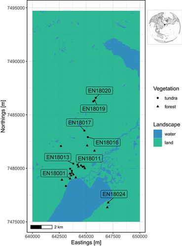
Our study region in central Chukotka (Northeast Siberia, Russia) is set up in the Lower Lake Ilirney area, at the northeastern margin of the northern tree line ecotone (Figure 1). It supports a wide range of vegetation types from relatively dense tree stands at lower elevations to tree-free prostrate lichen-dominated tundra generally at higher elevations (Shevtsova, Heim et al. 2020). According to field data collected in 2018 (Shevtsova, Kruse et al. 2020a), total AGB ranges from close to 0 kg m⁻² in the mountains (800–1,600 m.a.s.l.) to intermediate at around 0.56 kg m⁻² in the graminoid tundra (600–700 m.a.s.l. or in some places at lower elevations) and to around 2.48 kg m⁻² in the forest tundra (430–600 m.a.s.l.). The tree stands are formed solely of Larix cajanderi Mayr, which makes up the highest proportion of up to 60 percent of the total vegetation AGB on the forest tundra sites (Shevtsova et al. 2021). The typical climate for the area can be characterized as continental, with average January temperatures of −30°C, an average July temperature of +13°C, and annual precipitation of 200 mm year^–1 (Menne et al. 2012). The growing season is short (mean of around 100 days year⁻¹).

Figure 1. The study area of the Lake Ilirney system. Labels are given for field sites that are used to illustrate the simulation study results. Projection of the map is UTM58N.

Simulation set up

The dynamic forest model LAVESI

The Larix vegetation simulator (LAVESI) is an individual-based spatially explicit model that simulates larch stand dynamics (Kruse et al. 2016, 2018). It was set up to understand tree stand structure and migration and population dynamics of boreal forests growing between the leading edge of the Siberian tree line ecotone and the southern limit in response to a changing climate and its feedbacks with permafrost soils. The current version of LAVESI uses temperatures of the coldest and warmest months (January, July) and monthly precipitation series as climate forcing, as well as 6-hourly data on wind speed and direction and biological specifics of larch to simulate seed distribution and tree reproduction, growth, and death (Kruse et al. 2016, 2018, 2019). Recently, the model has been extended by including topography and landscape sensing of the individuals and additional boreal forest tree species (Picea obovata, Pinus sylvestris, Pinus sibirica) have been introduced alongside the larch species the model was initially developed for (Larix gmelinii, L. cajanderi, and L. sibirica; Kruse et al. 2022).

The model simulation area is variable in size and stores the specific biotic and abiotic environment. In the simulation areas, individual seeds and trees are exactly positioned by x, y coordinates. Simulation runs proceed in yearly time steps. To reach stabilization of population dynamics and the forcing climate series, simulations were preceded by a stabilization period that starts from bare ground, introducing seeds. To allow for repopulation of simulation areas after eventual extinction, some seeds are added every year to the simulation areas.

Each simulation starts with processing the weather data that are used to estimate maximum diameter growth (at basal and breast height) for each simulation year based on 10-year mean climate auxiliary variables. Within the growth processes of the model, these variables are used to individually estimate the current diameter growth of trees constrained by their actual biotic (competition) and abiotic (landscape features: elevation, topographical wetness index [TWI], slope, soil moisture, active layer depth) environment. This sets the actual basal diameter of each individual tree, which is used as the central state variable.

Within one simulation year, the following processes become consecutively invoked: Update of environment: Basal diameters of each individual tree are used to evaluate the competition strength. We use a yearly updated density map based on the basal diameter of each tree to pass information about competition for resources between trees. A litter layer, the active layer depth, and the state variables of each grid cell are updated as well. Growth: The individual growth of stem diameters is calculated from the maximum possible growth in the current year affected by the tree’s density index and its abiotic environment. From the resulting diameters, the tree height is estimated. Seed dispersal: Seeds in “cones” are dispersed from the parent trees, at a set rate. The dispersal directions and distances are randomly determined from a ballistic flight influenced by wind speed and direction, with decreasing probabilities for long distances and only to places lower than the release height. If dispersed seeds leave the extent of the simulated plot, they are removed from the system. Seed production: Trees produce seeds after the year at which they reached their stochastically estimated maturation height. The total amount depends on weather, competition, and tree size. Establishment: The seeds that lie on the ground germinate at a rate depending on current weather conditions, constrained by the actual litter layer height. Mortality: Individual trees or seeds die—that is, they are removed from the plot—at a specified mortality rate. For trees this is deduced from long-term mean weather values, a drought index, surrounding tree density, tree age and size, plus a background mortality rate. Seeds, on the other hand, have the same constant mortality rate whether on trees and or the ground. Aging: Finally, the age of seeds and trees increases once a year, and seeds are removed from the system when they reach a defined species age limit.

Updating of the model LAVESI

For LAVESI to simulate AGB dynamics at landscape scales representing a complex environment including mountainous topography, we made the following adjustments. We added elevation and environmental factors as new boundary conditions by using the slope angle and the TWI (see details in Appendixes 1 and 2). To convert from tree stand structure based on tree diameter growth to AGB, we implemented AGB equations (Appendix 3) and applied them to the simulated tree heights in LAVESI.

Simulation setup

We ran LAVESI simulations for three different Representative Concentration Pathway (RCP) climate scenarios (RCP 2.6, RCP 4.5, RCP 8.5 with and without cooling after 2300 CE) to see potential future paths of larch AGB change in the study region. Simulation runs were started with the topography- and biomass-implemented new LAVESI version with an empty landscape representing the true topography starting at 500 CE to allow for spin-up and ending in 2018 CE. Seeds (N = 100 000) for initiating the population establishment were introduced across a subset of 12 × 15 km in the southwestern corner of the simulation area (18 × 25 km) for the first fifty years. Only 1,000 seeds were introduced yearly after 550 CE, allowing for reestablishment after a complete die-out of trees had occurred on the whole simulated area.

The climate forcing was built as follows:

1. We extracted the historical climate data for the period 1901 to 2019 from the 0.5° × 0.5° Climate Research Unit gridded Time Series (CRU TS) monthly data (Harris et al. 2020; Figure 2) for the cell closest to Lake Ilirney (67.25° N, 128.25° E).

   Figure 2. Summer air temperature and yearly precipitation changes for the Ilirney lake system, central Chukotka, starting in the year 1700 CE with extrapolations according to different Representative Concentration Pathway (RCP) scenarios until 3000 CE.

   

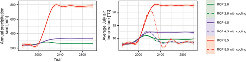
2. For the period 501 to 1900 CE we derived yearly air temperature from δ¹⁸O and precipitation from ice layer thickness series from the Severnaya Zemlya/AN ice core data (934–1998 CE; Opel, Fritzsche, and Meyer 2013). This series was extended to 501 CE by sampling twenty-five-year blocks of the yearly resolution data and adding this variability to data from the AN86/87 core (Arkhipov et al. 2008). Local adjustment was done by building linear models of yearly temperature and precipitation for the overlapping years 1901 to 1998 with the CRU TS data.

3. From the yearly data series, we built monthly data series by sampling fifteen-year-long blocks from available CRU TS data and adjusting the mean temperature by the difference of the sampled block from the estimated mean values.

4. For future climate forcings, we used a coupled climate model run output from Max Planck Institute Earth System Model (MPI-ESM) driven by three available RCP scenarios (Giorgetta et al. 2012a, 2012b, 2012c) from 2019 to 2300 CE. They were locally adjusted to the CRU TS data series using overlapping years. The resulting series were prolonged until 3000 CE by following the trend until 2500, subsequently keeping the temperature level reached at 2400 to 2500 until 3000 CE or, in the case of the cooling scenarios, we brought temperatures back to the years 1901 to 1987 CE of the series in a loop (Figure 2).

The wind data at 6-hourly resolution were extracted for 1979 to 2018 for the study region from the European Centre for Medium-Range Weather Forecasts (ECMWF) Re-Analysis ERA-Interim 0.75° × 0.75° (Dee et al. 2011). In simulation years not covered by this period, one year was randomly selected out of them to disperse seeds in all simulation years.

Model validation

Robustness of intersimulation results were tested with pairwise Pearson’s product-moment correlation (cor.test-function; R Core Team 2021) and with the standard deviation of three simulation repeats for simulation year 2020 CE.

To extract model parameters for landscape implementation and to validate simulation results, we established a reference data set (Appendix 2) based on modern high-resolution satellite data ESRI World Imagery (ESRI 2021). The simulated AGB values were processed to presence/absence data as well as the reference data set. Based on this, a confusion matrix was created stating the user’s accuracy, producer’s accuracy, and the overall accuracy following Stehman (1997). Based on these, we calculated kappa statistics and evaluated according to Landis and Koch (1977).

For a detailed validation of AGB state values and change, we extracted values from the following sources:

1. LAVESI simulations, resolution 30 × 30 m, AGB (oven-dry weight of all woody and leaf parts, kg m⁻²) for the years 2000, 2005, 2010, 2015, and 2020 CE. Additionally, per pixel uncertainty expressed as standard deviation in kilograms per square meter.

2. General additive model (GAM)-based regional product (Shevtsova et al. 2021) for study region, resolution 30 × 30 m, AGB (Larix fraction, oven-dry weight of all woody and leaf parts, kg m⁻²) for years 2001 and 2016 CE.

3. GLOBBIOMASS (global data sets of forest biomass, Santoro et al. 2022), resolution 38 × 99 m projected to UTM58; AGB (defined as the mass, expressed as oven-dry weight of the woody parts [stem, bark, branches, and twigs] of all living trees excluding stump and roots, tons ha⁻¹) for the year 2010 CE. Additionally, per pixel uncertainty expressed as standard error in tons per hectare.

4. European Space Agency Climate Change Initiative Biomass project (ESA CCI Biomass, Santoro and Cartus 2021), 38 × 99 m projected to UTM58; AGB (defined as the mass, expressed as oven-dry weight of the woody parts [stem, bark, branches, and twigs] of all living trees excluding stump and roots, tons ha⁻¹) for years 2010 and 2018 CE. Additionally, per pixel standard deviation of the AGB estimates in tons per hectare.

The extract function from the raster package in R (R Core Team 2021) was applied with a bilinear method for max value calculation of the closest four nearest neighboring cells to cope with spatial uncertainty.

The AGB change was calculated from fifteen simulation years (2015–2000 CE) covering a similar span as the products with available temporal data: GAM-based 2016–2001 CE, ESA CCI Biomass 2018–2010 CE. All data were brought to the same dimension of kilogram per square meter per year for comparison. A global root mean square error was used for the GAM-based data of 1.08 kg m⁻² and the standard deviation for the ESA CCI Biomass was extracted from a separate raster file. We compared individual data points of field locations present in both data sets as well as all data in overlapping areas by calculating Pearson’s product-moment correlation value.

All statistical analyses were performed in R 4.1.2 (R Core Team 2021), mostly using included standard functions, with additions from the package “raster” version 2.6–7 (Hijmans 2017) to treat and export raster AGB data and from “ggplot2” (Wickham 2016) for visualization of the results.

Processing model output

For plot-level change comparison we chose representative sites from the available data set at locations that are spatially homogeneous and do not fall in special landscape forms; for example, small-scale water accumulation zones. These were from three categories of contrasting vegetation presence as follows:

• Forest tundra sites: EN18001 and EN18024, which are located at an elevation of ~500 m.a.s.l. west and east, respectively, of the Lower Lake Ilirney with different slope direction characterized by medium-high biomass of larch trees present.

• Open graminoid (hummock) tundra: EN18011 and EN18013, close to the current forest edge at ~250 m and ~650 m distance, respectively. Both sites are located at an elevation of ~600 m.a.s.l. and, farther away, the sites EN18016 and EN18017 at an elevation of ~700 m.a.s.l., at 1.2 km and 1.8 km distance from the forest edge, respectively.

• Poorly vegetated open tundra sites with lichen communities, herbs, and dominant Dryas sp. EN18019 and EN18020 on rocky ground, both at an elevation of ~850 m.a.s.l., ~2.7 km from the forest edge.

To derive dynamics of forest and/or forest tundra in the study area under different climate scenarios for the simulated data from 2000 to 3000 CE, we used a threshold for biomass to assign forest tundra as opposed to open tundra in this region. Forest tundra has a minimum tree AGB of 0.68 kg m⁻² according to the 2018 field inventories (Shevtsova et al. 2021). Using this threshold, we calculated the percentage of areas with tree stands reaching this AGB level. We visualized results as the overall dynamics throughout the investigated period, as well as its spatial representation for selected years.

Results

Validation of the model’s performance

The simulation model produced robust results, and the intersimulation standard deviation of cells with larch growth in the simulation year 2020 CE had a median of 1.68e⁻⁰³ kg m⁻² (decreasing negatively exponentially in the range 1.73e⁻⁰⁸ to 1.40; N = 47,811 for the three simulation repeats; NA values that fall in water locations were 27,114 cells, total 191,667 cells). Correlation of cells with larch growth between the three repeat simulations was strong and highly significant (1 vs. 2, r = 0.961, t = 695.25; 1 vs. 3, r = 0.959, t = 678.86; 2 vs. 3, r = 0.960, t = 680.05; all p < .001).

Validation against the reference data set revealed an overall accuracy of 79 percent, and the general low number of cells with larches present was less accurate at 69.4 percent (Table 1). For this comparison, a kappa value of 0.405 suggests fair to moderate agreement of simulation with observation data. An ABG value comparison revealed that the simulation predicted systematically lower values than the GAM-based values (Figure 3a,c), which were within the estimated error range at all but one location that is outside the plus/minus root mean square error value of the model (1.08 kg m⁻²). Simulation was close to the direct observation (Figure 3g), though the value at the highest field location was underestimated. The other products performed similarly when taking into account the large errors associated with the data sets, or worse. The global data sets of forest biomass (GFD) presented no biomass at the compared locations but a large SD of 3.29 kg m⁻² (Figure 3b); GLOBBIOMASS had larger values that were in a similar range as the direct observations (Figures 3e,h); ESA CCI 2018 showed half as large values (Figure 3d) and roughly a constant value when compared to the direct observations (Figure 3i).

Figure 3. Aboveground biomass (AGB) values from fieldwork sites extracted from different sources and direct observations (a)–(i) and temporal changes (j)–(k). All values brought to the same unit (kg m⁻²) for comparison.

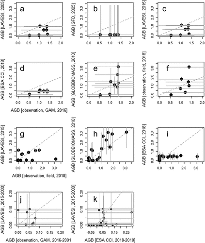
Table 1. Accuracy of predicted cells with larch presence and absence in comparison to observations.

	Observation
Prediction	Larch absent	Larch present	Sum	User’s accuracy (%)
Larch absent	1,641.0	128.0	1,769.0	92.8
Larch present	385.0	290.0	675.0	43.0
Sum	2,026.0	418.0	2,444.0
Producer’s accuracy (%)	81.0	69.4		79.0

The estimated temporal tree AGB change at a representative set of sites that can be extracted showed that the observed changes in larch AGB were generally very small over the fifteen years, which was well captured by the simulations (Table 2). The simulated rates of change in AGB were generally similar for all forest tundra sites (0.01–0.02 kg m⁻² year⁻¹) with one exception, where simulated tree AGB change was negative (EN18027). Field and Landsat-based estimations of tree AGB change were generally slightly lower or higher. The comparison of simulations to products showed that the simulations were characterized by a large variance but in the range of the errors of the products (Figure 3). The correlation coefficient between simulation and GAM-based extraction was 0.328 (p < 2.2⁻¹⁶, t_d.f.=31,012 = 61.109) and in the comparison to ESA CCI change values it was 0.269 (p < 2.2⁻¹⁶, t_d.f.=191,657 = 122.35).

Table 2. Change in larch aboveground biomass (AGB) estimated using simulation results from LAVESI and by using field and Landsat data from five forest tundra (ft) and one open tundra (ot) expedition sites, for which both field and Landsat-based AGB, as well as LAVESI-simulated tree AGB, are available.

Site	Larch AGB (kg m^−2)		Change in larch AGB (kg m^−2)		Estimated rate of change in larch AGB per year (kg m^−2 year^−1)
	LAVESI, 2015	LAVESI, 2000	LAVESI (2015–2000)	Field and Landsat-based (2016–2001)	LAVESI	Field and Landsat-based
EN18001 (ft)	1.274 ± 0.233	1.037 ± 0.247	0.237 ± 0.680	0.133	0.016 ± 0.045	0.009
EN18002 (ot)	0.004 ± 0.004	0.002 ± 0.002	0.002 ± 0.009	0.000	0.000 ± 0.001	0.000
EN18014 (ft)	0.859 ± 0.119	0.632 ± 0.107	0.228 ± 0.320	0.074	0.015 ± 0.021	0.005
EN18021 (ft)	0.021 ± 0.005	0.015 ± 0.005	0.006 ± 0.014	0.413	0.000 ± 0.001	0.028
EN18026 (ft)	1.206 ± 0.121	0.009 ± 0.006	1.196 ± 0.179	0.610	0.080 ± 0.012	0.041
EN18027 (ft)	0.017 ± 0.012	0.554 ± 0.068	−0.538 ± 0.113	0.047	−0.036 ± 0.008	0.003

Note. Variations show the standard deviation.

Plot-level AGB changes

Temporal changes in tree AGB had a similar character at both forested focus sites (Figure 4). In detail, under RCP 2.6, tree AGB generally increased in the first half of the twenty-first century, reaching its highest values of 1.5–1.6 kg m⁻², followed by a decrease until 2300 CE, with its lowest AGB of around 1 kg m⁻². From 2300 CE to 2700 CE the tree AGB fluctuated differently at the two investigated sites, showing an increase up to 1.5 kg m⁻² by around 2650 CE and gradual decrease afterward for EN18001 or a faster increase up to 1.3 kg m⁻² by around 2500 CE, fast decrease to 0.9 kg m⁻² by around 2650 CE, and fast increase again for EN18024. The fluctuations were similar under RCP 4.5, whereas under RCP 8.5 it took more time for larch AGB to reach its highest value; however, the values themselves fluctuated less, and for site EN18024 there was a clear increasing trend. In scenarios with cooling, tree AGB first increased until 2300 CE, reaching 1.5 to 1.6 kg m⁻², and then decreased gradually with fewer fluctuations, reaching around 0.75 kg m⁻², which was even less than that in 2000 CE (beginning of the investigation period). However, closer to 3000 CE under the warmest scenario RCP 8.5, a second tree AGB increase was simulated, which was not the case under RCPs 2.6 and 4.5.

Figure 4. Temporal changes in simulated larch aboveground biomass (AGB) of representative sites from 2000 to 3000 CE.

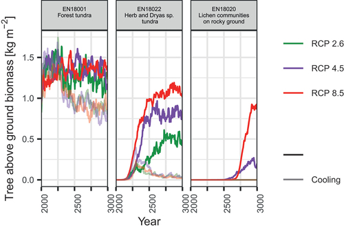
Tundra sites close to the current tree line had a similar trend as the forested sites except with a longer offset at the beginning (Figure 4). On the site closest to the current tree line (EN18011), the increase in tree AGB started from the 2000s, whereas on the site slightly farther away (EN18013), a strong increase in tree AGB was simulated to start later, after around 2100 CE. This trend was ongoing for sites EN18016 and EN18017 with the onset of AGB increase dated at around 2300 CE for the closer site, whereas at the latter, more distant site, the AGB increase started no earlier than after 2500 CE. Until stabilization, larch tree AGB steadily increased until 2250 CE for EN18011 and until 2500 CE for EN18013. After that, in both cases, tree AGB fluctuated around a certain value, depending on the RCP scenario. The highest values were reached under RCP 8.5 (1.1–1.3 kg m⁻²), moderate under RCP 4.5 (0.9–1.2 kg m⁻²), and lowest under RCP 2.6 (0.6–1 kg m⁻²). Under scenarios with cooling after 2300 CE, tree AGB, as at the currently forested sites, increased before cooling started and decreased afterward but, in contrast, typically stayed at higher values than at the beginning of the twenty-first century. On the site far from the tree line, tree AGB generally had lower values, and it took even longer for tree AGB to stabilize after increasing. Under cooling scenarios, tree AGB generally stayed close to 0 kg m⁻², rising before the cooling and dropping back to very low values after cooling.

On the two poorly vegetated tundra sites, the highest value of tree AGB was simulated to be around 1 kg m⁻² under RCP 8.5 (with no cooling; Figure 4). An increase was simulated only for the second half of the millennium and only under RCP scenarios 4.5 and 8.5 without cooling. If cooling occurred, tree establishment was disabled on both sites.

Landscape level AGB changes

The detailed observations at the plot level (Figure 5) depicted population dynamics that cause the spatial distribution and spreading of larch AGB. Following the simulations, larch AGB gradually increased, which was mostly associated with densification of existing tree stands until 2200 CE. Starting from 2200 CE, larch was simulated to spread more across the landscape, colonizing upslope areas. After 2400 CE for RCP 2.6, larch tree stands were simulated to become sparser, whereas establishment of larch tree stands continued in the newly colonized areas. The scales differed in the RCP scenarios: the highest values of tree AGB and the most northward spread were observed in RCP 8.5. Lowest values were simulated for scenarios with cooling after 2300 CE with larger larch cover but overall smaller AGB values (Figure 6).

Figure 5. Larch aboveground biomass (AGB) simulated for years 2020 to 3000 CE under three Representative Concentration Pathway (RCP) scenarios and for the final year under the cooling scenarios after 2300 CE. Forested areas with an AGB > 0.68 kg m² are given in percent in each plot.

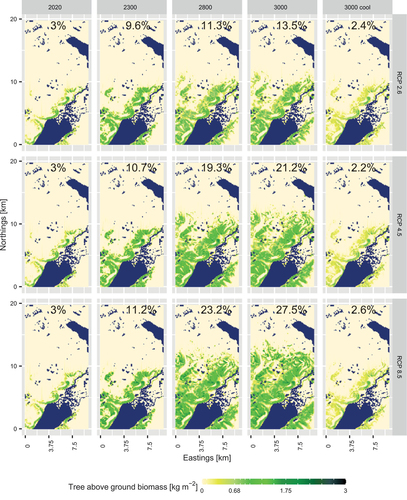
Figure 6. Simulations of temporal change in the study region under different climate scenarios until 3000 CE of total larch aboveground biomass (AGB).

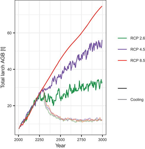
Changes in simulated larch AGB between 2020 and 3000 for most currently forested areas reached rates of 0.0005 to 0.002 kg m⁻² year⁻¹ (0.5–2 kg m⁻² per 980 years; Figure 5) depending on the RCP scenario, with the lowest under RCP 2.6 and the highest under RCP 8.5. Under scenarios with cooling, the rates of increase of mostly newly colonized areas did not exceed 0.0005 kg m⁻² year⁻¹ and of decrease for currently existing tree stands −0.0005 kg m⁻² year⁻¹. In the period until 2300 CE, all scenarios, with or without cooling, simulated a similar increase in tree AGB of up to 0.002 kg m⁻² year⁻¹.

The average (median) larch AGB across the whole study region in tundra for all scenarios was simulated to stay close to 0 kg m⁻² until around 2550 CE. From 2550 CE, it increased exponentially in the warm RCP 8.5 scenario, reaching 0.009 kg m⁻² by 3000 CE. The increase in larch AGB was delayed under RCP 4.5, reaching 0.0008 to 0.0009 kg m⁻² by 3000 CE. Under RCP 2.6, median larch AGB was simulated to stay around 0 kg m⁻² for the whole period. In the cooling scenarios, warming occurred only until 2300 CE, until when average (median) tree AGB in the region stayed close to 0 kg m⁻² in every case.

The average tree AGB rates of increase were strongest in the first 300 years of the third millennium but notably less for 2300 to 3000 CE (Table 3). With cooling after 2300 CE, tree AGB decreased from 2300 to 3000 CE at rates of −18.13 ± 0.19 (RCP 2.6), −23.46 ± 0.14 (RCP 4.5), and −25.25 ± 0.004 (RCP 8.5) t year⁻¹.

Table 3. Average tree aboveground biomass (AGB) rates of increase for different periods until 3000 CE under three Representative Concentration Pathway (RCP) scenarios.

RCP scenario	2020–2100 CE (t year^−1)	2100–2200 CE (t year^−1)	2200–2300 CE (t year^−1)	2300–3000 CE (t year^−1)
2.6	48.79 ± 0.32	60.68 ± 0.41	47.68 ± 0.44	15.56 ± 0.02
4.5	62.43 ± 0.21	47.73 ± 0.11	84.86 ± 0.16	39.31 ± 0.13
8.5	33.06 ± 0.07	100.06 ± 0.01	80.39 ± 0.81	63.52 ± 0.09

With respect to temporal and spatial dynamics of forest tundra in comparison to open tundra, our results showed that the higher the temperatures (e.g., RCP 8.5 vs. RCP 2.6), the higher the percentage of forested areas and the lower the fluctuations of this percentage during the investigated period (Figure 5). Under RCP 8.5, forest tundra was simulated to occupy up to 39 percent of the investigated region by the end (3000 CE), whereas under RCP 4.5 it was simulated to occupy around 33 percent of the whole investigated region, and under RCP 2.6 this estimate was up to around 25 percent (Figure 5). With the cooling scenarios, the highest percentage of forest tundra was reached in 2300 CE, which, depending on the RCP scenario, was 22 percent (RCP 2.6), 23 percent (RCP 4.5), or 24 percent (RCP 8.5). After cooling began, forested areas were simulated to decrease to 2 to 3 percent of the investigated region.

Discussion

Validation of simulations in comparison with aboveground biomass products

The LAVESI model slightly underestimated the simulated current larch AGB state (Figure 3), gave a wide range of recent temporal changes that fit to observations (Table 2), and accurately captured the general spatial distribution. However, as with many other spatially explicit models, it performed well at a general level but failed in reproducing some details (e.g., models used in Ito et al. 2020). In particular, the simulated amount of larch saplings (<2 m) was higher than observed during fieldwork, but it can differ greatly in nature from year to year (called high crop years; Abaimov et al. 1998). This was not considered by the model in which trees produced seeds depending on climate and available resources, but the small number of saplings observed during fieldwork could be a natural anomaly. The simulated larch AGB in kilograms per square meter on 15-m radius plots was generally similar to the field estimations, although values were underestimated for some field sites that had relatively high larch AGB from field estimations (Figure 3). Thus, in general, we can expect a higher larch AGB rate in some areas of the future landscape in the vicinity of the Ilirney lake system.

Using our model can highlight unrealistic AGB values from products and their associated spatially explicit errors, shown here for those provided by ESA CCI Biomass and GLOBBIOMASS. We showed that both overestimated the actual AGB, especially in places of complex terrain and high elevations. Here, values of 3 to 5 kg m⁻² were predicted in places with no vegetation at all, which could stem from the applied topographic correction of the utilized satellite data that did not sufficiently remove the artifact, as well as in wet areas partly covered with shrubs; it is a common phenomenon that vegetation in wet areas yields higher estimations than observed and is more often misinterpreted as tree cover. The authors of the GLOBBIOMASS product also stated in their description that their products are not applicable in our regions because they deliver only realistic values for regions with typical forest AGB >5 kg m⁻², which exceeds nearly all areas in our region of interest and high-latitude areas in general. For this purpose, the estimate for the region by Shevtsova et al. (2021) was established and should be used instead, although it is currently only available for a small region. One should be cautious, however, when using these or any biomass products, because the comparison of our simulations here showed that it is likely that the AGB values for the year 2001 CE were underestimates and hence produced a higher trend that would lead to deviance in the simulation results.

Although LAVESI simulations of the current status of tree AGB were mostly in accordance with tree stands depicted on a satellite image (Esri basemap), closer inspection revealed that several areas that currently have tree stands are not present in LAVESI and vice versa. Forests were not simulated in polygonal tundra, which is one of the most challenging areas because trees grow only on small rims typically not wider than a meter and were not captured by the digital elevation model (DEM) with its 90-m spatial resolution. Another common pattern of tree absence in LAVESI simulations was for the forested areas of steep slopes where a transition from forest tundra to pine shrub tundra and graminoid tundra also occurred. This was probably owing to the topography models used to modulate larch occurrence and could be improved by further parameterization. Herbivory could also be a factor constraining growth at these tree line ecotone margins because reindeer affect regrowth or fitness (Cairns and Moen 2004; Mienna et al. 2020; Rees et al. 2020). Furthermore, an implementation of biotic factors such as competition between larch and pine in the model can provide better accuracy in the larch distribution. However, errors in forest structure were found to have stronger effects on tree growth projections than errors in species composition (Falkowski et al. 2010).

Forest development under warming climate

With the topography and biomass-implemented LAVESI model we could simulate larch AGB dynamics (general increase) and forest spreading upwards and northwards along elevational and latitudinal gradients. Further, we revealed that forests did not recede from colonized areas even when hypothetical cooling to twentieth-century levels prevailed until the end of the millennium. Current tree stands started to noticeably expand upslope around 2200 CE (Figure 5). As expected, highest rates of forestation from today until 3000 CE (Figure 6) were simulated under RCP 8.5. In every scenario we could see a gradual increase in larch AGB by the end of the investigated period. There were fluctuations in areas that were already forested by 2020 and in sites closer to the current tree line, revealing typical population dynamics. On the open tundra plots with graminoid vegetation and close to the tree line, we observed larch colonizing new areas upslope with a time lag (starting after 100–500 years depending on the position of the site), where after the arrival of seeds, saplings developed, and in the next stage a cohort was established. Once trees established under warming, tree AGB developed exponentially. When comparing population dynamics in the different RCP scenarios at the beginning of the twenty-first century, there was clear self-thinning of the tree stands (strongly prominent under the warmest climate conditions of RCP 8.5), which can be explained by strong individual tree competition (as in Wieczorek et al. 2017 for the Taimyr Peninsula).

The simulation showed a first general increase (and stabilization in the next centuries) in tree AGB in the subarctic region, even under RCP 2.6 where air temperature and precipitation changes were the smallest, and a higher increase of tree AGB under RCPs 4.5 and 8.5. These results are in accordance with previous findings that vegetation changes were initiated during the past three decades of changing climate conditions and might be expected to be even greater with additional greenhouse gases in the atmosphere (Callaghan and Carlsson 1997). However, tree lines worldwide respond differently depending on various local conditions (Harsch et al. 2009). In comparison with recent (2000–2015) larch AGB change rates (0.006 kg m⁻² year⁻¹) in the upper tree line zone of another Russian subarctic mountainous tree line ecotone (Polar Ural; Devi et al. 2020), simulated recent (2000–2015) larch AGB change rates (0.016–0.08 kg m⁻² year⁻¹) on most forest tundra sites were faster in our study region.

Until the end of the twenty-first century, our simulations of forest expansion showed that forest tundra covers less than 20 percent (areas with tree AGB > 0.68 kg m⁻²), which is in line with other simulations. Unfortunately, a direct comparison is impeded because, to date, no high-resolution and spatially explicit simulations are available, which are necessary for the complex terrain of the study area. Nevertheless, for illustration, we compared the data to results from global vegetation models (Sitch et al. 2008) and observed no or much lower (1–20 percent) changes in tree cover in our study area compared to two other global vegetation models, which showed an increase in tree cover from 20 to 50 percent and higher in central Chukotka over the same period. Regional simulations, still at a coarse but higher resolution of 23 × 23 km, were provided by applying UVAFME (an individual tree-based gap model set up for large regions; Shuman, Shugart, and Krankina 2014; Shuman et al. 2015, 2017) in the northern taiga of Chukotka (closest area to our investigated region; scenario without fire; Shuman et al. 2017). The results for 2100 CE showed a general larch AGB of the forested areas in the tundra–taiga reaching 0.5 to 2.5 kg m⁻², which is similar to our simulations, whereas south of our study region in northern taiga it is around 1–20 kg m⁻² total larch biomass. The latter stand densities could be reached by forests in our study region only when global warming proceeded unstopped, sequestering carbon but also reducing the albedo (Bonan 2008).

Time-lagged maximum forest expansion and retreat under cooling climate

The time required for simulated tree stands to respond to climate changes (time lag) was shortest for the RCP 8.5 scenario, which is about 500 years when considering the region of investigation as a whole but smaller when considering different parts of the region. For the currently forested sites, an exponential increase already began at the beginning of the investigated period (2000s) and took about 50 years to reach a stable state, whereas after cooling, the decrease took at least 500 years to stabilize. On the open tundra sites, both processes took longer, but tree stand establishment (300–375 years) still occurred faster than tree stand dieback (450 years or more). At the currently sparsely vegetated sites, tree establishment generally did not reach a stabilization phase until the end of the investigated period, which led to faster diebacks when cooling occurs. We also observed a time lag of about 200 years in the cooling scenarios after the cooling event. At the stand-level scale, tree AGB generally declined at the onset of cooling, which indicates tree stand thinning. Areas that were not colonized until the end of the warming phase leading to tundra invasion became deforested in scenarios with cooling. This could be an opportunity for tundra areas to survive global warming. However, for the region in general, although the decline in tree AGB in the first century after cooling was steeper than warming-induced tree AGB increase before cooling, our results also showed that once tundra became colonized by forests, the forests could survive longer during the following cooling phase and not change back to tundra until the end of the simulation.

Our results without cooling were in accordance with Chapin and Starfield (1997), who concluded that regardless of warming rate, there will be substantial lags in forest expansion (150–250 years in Alaska for 5 percent of forest establishment), and other models that also simulated time-lagged vegetation change, highlighting migration and succession processes (Epstein et al. 2007). Further, our simulated future changes in vegetation agree with previously investigated ecosystem parameters. For example, Zhang et al. (2013) simulated no change in albedo or latent heat flux until 2080 in central Chukotka, particularly in the Ilirney lakes area. This is in general agreement with our simulations of time-lagged tree AGB, which, although increasing until 2080 CE, would probably cause differences in albedo and latent heat flux too weak to be captured by a global model such as the one Zhang et al. (2013) used.

The observation of small remnants of larch individuals ahead of the tundra even after cooling and its associated general retreat of the tree line was nonlinear and the slower, or lack of, dieback of the forests challenges necessary tundra conservation. We deduced from our simulations that places of former tundra may not revert back to the different tundra types under improving climate conditions as easily as they were colonized. This phenomenon of slower retreat than expected has been shown on tree line–to-shoreline long transect simulations with LAVESI (Kruse and Herzschuh 2022). Out of these refugia populations, full-grown forests can reestablish much quicker than from bare ground as in the beginning of the twenty-first century and threaten the special species composition adapted to tree-free areas for millions of years (Arctic Climate Impact Assessment 2004; Schmidt et al. 2017). This highlights once again that conservation of the tundra areas will be a challenge in this complex system: the most promising measure would be to limit global warming as much as possible to prevent tundra areas from becoming forests in the first place.

Conclusions

The LAVESI model simulates an increase in larch AGB and tree line advance into the tundra (upslope and northwards) in central Chukotka until 3000 CE under RCP scenarios 2.6, 4.5, and 8.5 without cooling after 2300 CE. In scenarios with cooling, rapid tree stand thinning is observed and a decrease in total tree AGB in the currently forested areas to quantities lower than present. However, the areas occupied by forest tundra after cooling are simulated to cover larger areas than in 2000.

For currently forested areas, we simulate more fluctuations in tree AGB following typical tree stand structure development with densification, stabilization, and tree stand thinning processes. For nonforested areas, we simulate the same pattern of ecological development but time-lagged because of the time required for tree establishment in the open areas. For open tundra tree stands, establishment is simulated to start after 100 to 500 years depending on the distance to the current tree line. The average rates of AGB change are higher in the first 300 years of the twenty-first century and become lower toward 3000 CE. With a cooling event, the highest possible forest expansion is simulated to reach not more than 10 percent of the investigated region, and tree AGB for the whole region decreases from 2300 to 3000 CE. Time-lagged changes in tree AGB can be the key to preventing forestation in some areas of the tundra–taiga while managing CO₂ concentrations and thus temperature to restrict forest tundra from expanding further into the tundra.

The revealed nonlinear responses to climate forcing, especially the slower than expected dieback of forests and retention of larch individuals in low numbers in former and potentially future tundra areas, are threatening the special composition of plant communities in these places. With the vegetational changes, the necessary habitats for cold-adapted animals may get lost, which will have a profound impact on tundra biodiversity in a future climate. Preventing forest invasion in the first place seems to be the best measure to conserve tundra areas in a complex landscape.

LAVESI can simulate larch AGB values at the landscape level, reflecting patterns of current tree stand distribution fairly well, but slightly underestimates the observed values of tree AGB, which could be improved in the future. A comparison with other studies revealed some agreements as well as disagreements. LAVESI can reveal nonlinear changes and accurately predict tree distribution, which would not be possible with a simple predictive model using climate envelopes for species presence/absence.

Author contributions

SK, UH, and IS designed the study. SK developed the LAVESI model. Field data were collected on expedition, planned, organized, and coordinated by UH, LP, SK, and EZ. IS processed the field data, performed the validation study, and started simulations with LAVESI. IS drafted the first version of the article, which was jointly edited by all authors.

Acknowledgments

We thank Cathy Jenks for proofreading and improving the article. We also acknowledge the editor and two anonymous reviewers who provided critical comments that led to the improved version of the article.

Disclosure statement

The authors declare that the research was conducted in the absence of any commercial or financial relationships that could be construed as a potential conflict of interest.

Data availability statement

The source code of the new LAVESI version used in this study is publicly available on GitHub (https://github.com/StefanKruse/LAVESI/tree/ChukotkaBiomassSims) and is permanently stored on Zenodo (Kruse 2023). Materials used for parameterization and validation for the region of interest can be found on Zenodo: stratified sampled landscape classes (Shevtsova et al. 2023b) and forest density estimates (Shevtsova et al. 2023a). The simulation results are available online on Zenodo: simulated aboveground biomass of forests (Shevtsova et al. 2023d), total AGB of the region of interest (Shevtsova et al. 2023c), and total forest cover percentages (Shevtsova et al. 2023e).

Supplementary material

Supplemental data for this article can be accessed online at https://doi.org/10.1080/15230430.2023.2220208.

Additional information

Funding

This study was supported by the German Federal Ministry of Education and Research (BMBF), which enabled the Russian–German research programme “Kohlenstoff im Permafrost KoPf” (Grant No. 03F0764A); by the Initiative and Networking Fund of the Helmholtz Association; and by the ERC consolidator grant Glacial Legacy of Ulrike Herzschuh (Grant No. 772852).

Appendix 1.

Implementing topographical parameters: Elevation, aspect, slope angle, and topographical wetness index

Topography modulates regional climate and controls the spatial patterns of the tree line limits (Holtmeier and Broll 2009). We used the TanDEM-X 90-m DEM product (Krieger et al. 2013) to extract the relevant spatial topographical parameters, namely, elevation, slope angle, and TWI. Prior to extraction of spatial topographical parameters, the DEM was resampled from the 90-m cell spacing to a 30-m resolution with bilinear interpolation. We also investigated aspect, but when evaluating the topographical parameters for implementation, it did not have a strong effect. Slope angle and aspect were calculated in SAGA 2.3.2 (Conrad et al. 2015; as QGIS 3.16.0 plugin) using Zevenberger and Thorne’s second-order polynomial adjustment algorithm (Zevenbergen and Thorne 1987). The TWI represents the moisture content, spatially distributed across the landscape. The TWI was calculated using the basic terrain analysis tool (SAGA GIS plugin) with the default setting of “the channel density” set to five. The final topography layers—elevation, slope angle, and TWI—were masked for areas of present surface water, such as Lower and Upper Lake Ilirney, small ponds, and rivers. We created the water mask by applying the land–water threshold technique to the Landsat-8 shortwave infrared 1 band (water reflectance <600) on a summer acquisition on 12 July 2018 with the Landsat spatial resolution of 30 m.

The topographical data (elevation, slope angle, TWI) were introduced in the source code of LAVESI as 30 × 30 m gridded input data, featuring a user-defined area. Based on this, the values were linearly interpolated to the internally used environmental grid of 20 × 20 cm tiles.

The seed dispersal, which already depended on wind direction and speed, release height, and species-specific fall rates (Kruse et al. 2018, 2019), was further improved for this study by shortening the upslope dispersal distance and restricting it to locations below release height.

Appendix 2.

Parameterization of the influence of topography and wetness on tree presence and growth

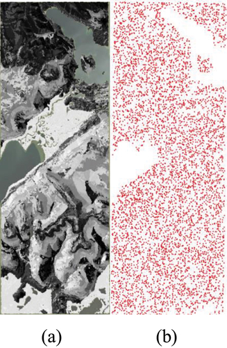
To extract the dependence of tree presence from the topographic parameters—aspect, slope angle, and topographical wetness index (TWI)—we used a high-resolution satellite acquisition from early summer in 2010 (ESRI World Imagery), which allowed identification of single trees and covering a representative part of the study region. In the first step, 6,488 sampling points for evaluation of the presence of trees were selected by stratified random sampling from 589 different possible combinations of elevation, slope angle, aspect, and TWI (Figure 2.1a; Table 2.1). The samples covered 2 percent of the area (Figure 2.1b), from southern forested areas via hummock tundra to the nonvegetated northern mountainous areas.

Table 2.1. Stratified random sampling categories.

Elevation	Slope	Aspect
0–400 m 400–450 m 450–500 m 500–600 m 600–650 m 650–700 m 700–1000 m 1000–1500 m	0–2° 2–4° 4–6° 6–8° 8–10° 10–12° 12–16° 16–18° 18–20° 20–25° 25–50°	0–45° 45–90° 90–135° 135–180° 180–225° 225–270° 270–315° 315–360°

Note. To conduct stratified random sampling, we used all possible combinations of elevation, slope, and aspect with breakpoints, forming the following categories.

Figure 2.1. (a) Visualization of the combinations of elevation, slope angle, and topographical wetness index (TWI) in the area for parameterization of the new topographic components in LAVESI with 589 categories distinguished, shown in gray shades, and (b) 6488 samples, marked as red dots.

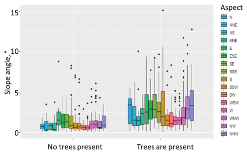
A visual assessment of the established relationship showed that aspect does not play an important role in the presence of trees in the study region (Figure 2.2). Areas both with and without trees showed the same pattern of sample distributions in relation to the aspect data. In contrast, one can clearly see that trees prefer higher slope angles, rather than lower.

Figure 2.2. Tree presence depends strongly on slope angle and very slightly on aspect in the study region (based on 6,488 stratified random samples). The patterns of aspect and slope angle combinations are generally similar for each direction of the treeless and tree areas, whereas areas with trees are found on slopes with higher angles in comparison to treeless areas for most of the aspect directions.

As a consequence, we could separately establish two statistically significant linear models predicting tree presence (in percentage of observations) depending on slope angle and TWI:

(2.1) $\mathit{TrPrSA}=e^{-0.5\frac{{(\mathit{slope}\mathit{angle}-\mathit{a})}^2}{b^2}}=e^{-0.5\frac{{(\mathit{slope}\mathit{angle}-12.58)}^2}{{12.78}^2}},$(2.1)

where TrPrSA is tree presence depending on slope angle, and a and b are coefficients (Table 2.2).

(2.2) $\mathit{TrPrT}=-\mathit{c}\ast \mathit{TWI}+0.98=-0.05\ast \mathit{TWI}+0.98,$(2.2)

where TrPrT is tree presence depending on TWI, and c is a coefficient (Table 2.2).

The models have good accuracy with residual standard errors of 0.013 (model under formula 3) and 0.011 (model under formula 4) and all significant coefficients (Tables 2.2 and 2.3).

The coefficients of these models were introduced into the model LAVESI to control environmental impact on individual growth simply by using the predicted forest presence at a certain location as a factor for the actual individual tree growth:

(2.3) $\mathit{Envirgrowth}=0.5\mathit{TrPrT}+0.5e^{2\mathit{TrPrSA}}$(2.3)

Table 2.2. Permutation test results for tree presence versus slope angle with three coefficients and their significance levels.

	Estimate	Standard error	t Value	Pr(>|t|)
a	12.580	1.076	11.685	<.0001
b	12.781	1.377	9.281	<.0001

Table 2.3. Permutation test results for tree presence versus topographical wetness index (TWI) with an intercept, one coefficient, and their significance levels.

	Estimate	Standard error	t Value	Pr(>|t|)
Intercept	0.980	0.045	21.879	<.0001
c	−0.050	0.005	−9.955	<.0001

Appendix 3.

Calculation of aboveground biomass (AGB)

To predict the AGB of each of the simulated larch trees, we used two separate models for needle and woody biomass established previously for the field sites in the study region (Shevtsova et al. 2021) based on a set of sampled trees (Shevtsova, Kruse et al. 2020a) and simplified to estimate the biomass of all trees on the sites based on the recorded height of the present trees (Kruse et al. 2020). Needle biomass of a living tree was calculated from the LAVESI-simulated tree height as follows:

(3.1) $\mathit{AGBn}=\frac{703.62}{1+{\mathit{e}}^{-\frac{\mathit{H}-579.5}{208.69}}}(\mathit{g}),$(3.1)

where $\mathit{H}$ is tree height (cm). Wood biomass from a LAVESI-simulated living tree was calculated as follows:

(3.2) $\mathit{AGBwl}=\frac{78713.63}{1+{\mathit{e}}^{-\frac{\mathit{H}-793.64}{73.91}}}(\mathit{g}).$(3.2)

References

- Abaimov, A. P., J. A. Lesinski, O. Martinsson, and L. I. Milyutin. 1998. Variability and ecology of Siberian larch species. Report 43. Umeå: Swedish University of Agricultural Sciences, Department of Silviculture.
- Arctic Climate Impact Assessment. 2004. Impacts of a warming Arctic-Arctic climate impact assessment. Cambridge, UK: Cambridge University Press.
- Arkhipov, S. M., V. Kotlyakov, Y.-M. K. Punning, V. Zogorodnov, V. I. Nikolayev, V. S. Zagorodnov, Y. Y. Macheret, et al. 2008. Deep drilling of glaciers: Russian projects in the Arctic (1975-1995). Moscow, PANGAEA: Institute of Geography, Russian Academy of Sciences. doi:10.1594/PANGAEA.707363.
- Bergengren, J. C., S. L. Thompson, D. Pollard, and R. M. DeConto. 2001. Modeling global climate–vegetation interactions in a doubled CO2 world. Climatic Change 50, no. 1/2: 31–20. doi:10.1023/A:1010609620103.
- Bonan, G. B. 2008. Forests and climate change: Forcings, feedbacks, and the climate benefits of forests. Science 320, no. 5882: 1444–9. doi:10.1126/science.1155121.
- Bonan, G. B., F. S. Chapin, and S. L. Thompson. 1995. Boreal forest and tundra ecosystems as components of the climate system. Climatic Change 29, no. 2: 145–67. doi:10.1007/BF01094014.
- Bonan, G. B., S. Levis, S. Sitch, M. Vertenstein, and K. W. Oleson. 2003. A dynamic global vegetation model for use with climate models: Concepts and description of simulated vegetation dynamics. Global Change Biology 9, no. 11: 1543–66. doi:10.1046/j.1365-2486.2003.00681.x.
- Cairns, D. M., and J. Moen. 2004. Herbivory influences tree lines. Journal of Ecology 92, no. 6: 1019–24. doi:10.1111/j.1365-2745.2004.00945.x.
- Callaghan, T. V., B. A. Carlsson. 1997. Impacts of climate change on demographic processes and population dynamics in Arctic plants. In Global change and Arctic terrestrial ecosystems, ed. W. C. Oechel, T. V. Callaghan, T. Gilmanov, J. I. Holten, B. Maxwell, U. Molau, and S. B, 201–14. Dordrecht: Springer.
- Chapin, F. S., and A. M. Starfield. 1997. Time lags and novel ecosystems in response to transient climatic change in Arctic Alaska. Climatic Change 35, no. 4: 449–61. doi:10.1023/A:1005337705025.
- Conrad, O., B. Bechtel, M. Bock, H. Dietrich, E. Fischer, L. Gerlitz, J. Wehberg, V. Wichmann, and J. Böhner. 2015. SAGA: System for Automated Geoscientific Analyses (SAGA) v. 2.1.4. Geoscientific Model Development 8: 1991–2007. doi:10.5194/gmd-8-1991-2015.
- Dee, D. P., S. M. Uppala, A. J. Simmons, P. Berrisford, P. Poli, S. Kobayashi, U. Andrae, et al. 2011. The ERA-Interim reanalysis: Configuration and performance of the data assimilation system. Quarterly Journal of the Royal Meteorological Society 137, no. 656: 553–97. doi:10.1002/qj.828.
- Devi, N. M., G. А. A. Kukarskih VV, А. A. Galimova, V. S. Mazepa, and A. A. Grigoriev. 2020. Climate change evidence in tree growth and stand productivity at the upper treeline ecotone in the Polar Ural Mountains. Forest Ecosystems 7, no. 1: 7. doi:10.1186/s40663-020-0216-9.
- Druel, A., P. Clais, G. Krinner, and P. Peylin. 2019. Modeling the vegetation dynamics of northern shrubs and mosses in the ORCHIDEE land surface model. Journal of Advances in Modeling Earth Systems 11, no. 7: 2020–35. doi:10.1029/2018MS001531.
- Epstein, H., Q. Yu, J. Kaplan, and H. Lischke. 2007. Simulating future changes in Arctic and subarctic vegetation. Computing in Science & Engineering 9, no. 4: 12–23. doi:10.1109/MCSE.2007.84.
- ESRI. 2021. High-resolution satellite and aerial imagery, typically within 3-5 years [ basemap]. Scale not given. “ basemap”. https://www.arcgis.com/home/item.html?id=10df2279f9684e4a9f6a7f08febac2a9 (accessed December 15, 2020).
- Falkowski, M. J., A. T. Hudak, N. L. Crookston, P. Gessler, E. H. Uebler, and A. Smith. 2010. Landscape-scale parameterization of a tree-level forest growth model: A k-nearest neighbour imputation approach incorporating LiDAR data. Canadian Journal of Forest Research 40, no. 2: 184–99. doi:10.1139/X09-183.
- Foley, J. A., S. Levis, I. C. Prentice, D. Pollard, and S. L. Thompson. 1998. Coupling dynamic models of climate and vegetation. Global Change Biology 4, no. 5: 561–79. doi:10.1046/j.1365-2486.1998.t01-1-00168.x.
- Foster, A. C., A. H. Armstrong, J. K. Shuman, H. H. Shugart, B. M. Rogers, M. C. Mack, S. J. Goetz, and J. K. Ranson. 2019. Importance of tree- and species-level interactions with wildfire, climate, and soils in interior Alaska: Implications for forest change under a warming climate. Ecological Modelling 409: 108765. doi:10.1016/j.ecolmodel.2019.108765.
- Gamache, I., and S. Payette. 2004. Height growth response of tree line black spruce to recent climate warming across the forest-tundra of eastern Canada. Journal of Ecology 92, no. 5: 835–45. doi:10.1111/j.0022-0477.2004.00913.x.
- Giorgetta, M., J. Jungclaus, C. Reick, S. Legutke, V. Brovkin, T. Crueger, M. Esch, K. Fieg, K. Glushak, V. Gayler, et al. 2012a. CMIP5 simulations of the Max Planck Institute for Meteorology (MPI-M) based on the MPI-ESM-LR model: The rcp26 experiment, served by ESGF. World Data Center for Climate (WDCC) at DKRZ. doi:10.1594/WDCC/CMIP5.MXELr2.
- Giorgetta, M., J. Jungclaus, C. Reick, S. Legutke, V. Brovkin, T. Crueger, M. Esch, K. Fieg, K. Glushak, V. Gayler, et al. 2012b. CMIP5 simulations of the Max Planck Institute for Meteorology (MPI-M) based on the MPI-ESM-MR model: The rcp45 experiment, served by ESGF. World Data Center for Climate (WDCC) at DKRZ. doi:10.1594/WDCC/CMIP5.MXMRr4.
- Giorgetta, M., J. Jungclaus, C. Reick, S. Legutke, V. Brovkin, T. Crueger, M. Esch, K. Fieg, K. Glushak, V. Gayler, et al. 2012c. CMIP5 simulations of the Max Planck Institute for Meteorology (MPI-M) based on the MPI-ESM-MR model: The rcp85 experiment, served by ESGF. World Data Center for Climate (WDCC) at DKRZ. doi:10.1594/WDCC/CMIP5.MXMRr8.
- Harris, I., T. J. Osborn, P. Jones, and D. Lister. 2020. Version 4 of the CRU TS monthly high-resolution gridded multivariate climate dataset. Scientific Data 7, no. 1. doi:10.1038/s41597-020-0453-3.
- Harsch, M. A., P. E. Hulme, M. S. McGlone, and R. P. Duncan. 2009. Are treelines advancing? A global meta-analysis of treeline response to climate warming. Ecology Letters 12, no. 10: 1040–9. doi:10.1111/j.1461-0248.2009.01355.x.
- Hijmans, R. J. 2017. Raster: Geographic data analysis and modeling, R package version 2.6-7. https://CRAN.R-project.org/package=raster
- Holland, M. M., and C. M. Bitz. 2003. Polar amplification of climate change in coupled models. Climate Dynamics 21, no. 3–4: 221–32. doi:10.1007/s00382-003-0332-6.
- Holtmeier, F.-K., and G. Broll. 2009. Altitudinal and polar treelines in the northern hemisphere causes and response to climate change. Polarforschung 79: 139–53. http://hdl.handle.net/10013/epic.35706.d001
- IPCC. 2014. Climate change 2014: Synthesis report. Contribution of working groups I, II and III to the Fifth Assessment Report of the Intergovernmental Panel on Climate Change [Core Writing Team, Pachauri RK & Meyer LA (eds.)]. 151. Geneva, Switzerland: IPCC.
- IPCC. 2021. Climate change 2021: The physical science basis. Contribution of working group I to the Sixth Assessment Report of the Intergovernmental Panel on Climate Change [Masson-Delmotte V, Zhai P, Pirani A, Connors SL, Péan C, Berger S, Caud N, Chen Y, Goldfarb L, Gomis MI, Huang M, Leitzell K, Lonnoy E, Matthews JBR, Maycock TK, Waterfield T, Yelekçi O, Yu R & Zhou B (eds.)]. Cambridge University Press. In Press.
- Ito, A., R. Cpo, A. Gädeke, P. Ciais, J. Chang, M. Chen, L. François, et al. 2020. Pronounced and unavoidable impacts of low-end global warming on northern high-latitude land ecosystems. Environmental Research Letters 15, no. 4: 44006. doi:10.1088/1748-9326/ab702b.
- Kagawa, A., D. Naito, A. Sugimoto, and T. C. Maximov. 2003. Effects of spatial and temporal variability in soil moisture on widths and δ13C values of eastern Siberian tree rings. Journal of Geophysical Research 108, no. D16: 4500. doi:10.1029/2002JD003019.
- Kirilenko, A. P., and A. M. Solomon. 1998. Modeling dynamic vegetation response to rapid climate change using bioclimatic classification. Climatic Change 38, no. 1: 15–49. doi:10.1023/A:1005379630126.
- Krieger, G., M. Zink, M. Bachmann, B. Bräutigam, D. Schulze, M. Martone, P. Rizzoli, et al. 2013. TanDEM-X: A radar interferometer with two formation-flying satellites. Acta Astronautica 89: 83–98. doi:10.1016/j.actaastro.2013.03.008.
- Kruse, S. 2023. StefanKruse/LAVESI: LAVESI-WIND with landscape (v2.0). Zenodo. doi:10.5281/zenodo.7505539.
- Kruse, S., A. Gerdes, N. J. Kath, L. S. Epp, K. R. Stoof-Leichsenring, L. A. Pestryakova, and U. Herzschuh. 2019. Dispersal distances and migration rates at the Arctic treeline in Siberia—A genetic and simulation-based study. Biogeosciences 16, no. 6: 1211–24. doi:10.5194/bg-16-1211-2019.
- Kruse, S., A. Gerdes, N. J. Kath, and U. Herzschuh. 2018. Implementing spatially explicit wind-driven seed and pollen dispersal in the individual-based larch simulation model: LAVESI-WIND 1.0. Geoscience Model Development 11, no. 11: 4451–67. doi:10.5194/gmd-11-4451-2018.
- Kruse, S., and U. Herzschuh. 2022. Regional opportunities for tundra conservation in the next 1000 years. eLife 11: e75163. doi:10.7554/eLife.75163.
- Kruse, S., U. Herzschuh, L. Schulte, S. M. Stuenzi, F. Brieger, E. S. Zakharov, and L. A. Pestryakova. 2020. Forest inventories on circular plots on the expedition Chukotka 2018, NE Russia. PANGAEA. doi: 10.1594/PANGAEA.923638.
- Kruse, S., S. M. Stuenzi, J. Boike, M. Langer, J. Gloy, and U. Herzschuh. 2022. Novel coupled permafrost–forest model (LAVESI–CryoGrid v1.0) revealing the interplay between permafrost, vegetation, and climate across eastern Siberia. Geoscientific Model Development 15, no. 6: 2395–422. doi:10.5194/gmd-15-2395-2022.
- Kruse, S., M. Wieczorek, F. Jeltsch, and U. Herzschuh. 2016. Treeline dynamics in Siberia under changing climates as inferred from an individual-based model for Larix. Ecological Modelling 338: 101–21. doi:10.1016/j.ecolmodel.2016.08.003.
- Landis, J. R., and G. G. Koch. 1977. The measurement of observer agreement for categorical data. Biometrics 33, no. 1: 159–74. doi:10.2307/2529310.
- Liang, M., A. Sugimoto, S. Tei, T. Bragin IV, S. Morozumi, T. Shingubara, R. Maximov, K. S. I. TC, T. A. Velivetskaya, and A. V. Ignatiev. 2014. Importance of soil moisture and N availability to larch growth and distribution in the Arctic taiga-tundra boundary ecosystem, northeastern Siberia. Polar Science 8, no. 4: 327–41. doi:10.1016/j.polar.2014.07.008.
- Menne, M. J., I. Durre, B. Korzeniewski, S. McNeal, K. Thomas, X. Yin, S. Anthony, et al. 2012. Global Historical Climatology Network - Daily (GHCN-Daily), Version 3. National Centers for Environmental Information, NESDIS, NOAA, U.S. Department of Commerce. doi:10.7289/V5D21VHZ.
- Mienna, I. M., J. D. M. Speed, K. Klanderud, G. Austrheim, E. Næsset, and O. M. Bollandsås. 2020. The relative role of climate and herbivory in driving treeline dynamics along a latitudinal gradient. Journal of Vegetation Science 31, no. 3: 392–402. doi:10.1111/jvs.12865.
- Miller, G. H., R. B. Alley, J. Brigham-Grette, J. J. Fitzpatrick, L. Polyak, M. Serreze, and J. W. C. White. 2010. Arctic amplification: Can the past constrain the future? Quaternary Science Reviews 29, no. 15–16: 1779–90. doi:10.1016/j.quascirev.2010.02.008.
- Opel, T., D. Fritzsche, and H. Meyer. 2013. Eurasian Arctic climate over the past millennium as recorded in the Akademii Nauk ice core (Severnaya Zemlya). Climate of the Past 9, no. 5: 2379–89. doi:10.5194/cp-9-2379-2013.
- R Core Team. 2021. R: A language and environment for statistical computing. Vienna, Austria: R Foundation for Statistical Computing. https://www.R-project.org/
- Rees, W. G., A. Hofgaard, S. Boudreau, D. M. Cairns, K. Harper, S. Mamet, I. Mathisen, Z. Swirad, and O. Tutubalina. 2020. Is subarctic forest advance able to keep pace with climate change? Global Change Biology 26, no. 7: 3965–77. doi:10.1111/gcb.15113.
- Rupp, T. S., F. S. Chapin, and A. M. Starfield. 2000. Response of subarctic vegetation to transient climatic change on the Seward Peninsula in north‐west Alaska. Global Change Biology 6, no. 5: 54–555. doi:10.1046/j.1365-2486.2000.00337.x.
- Santoro, M., and O. Cartus. 2021. ESA Biomass Climate Change Initiative (Biomass_cci): Global datasets of forest above-ground biomass for the years 2010, 2017 and 2018, v3. NERC EDS Centre for Environmental Data Analysis. doi:10.5285/5f331c418e9f4935b8eb1b836f8a91b8.
- Santoro, M., O. Cartus, S. Mermoz, A. Bouvet, T. Le Toan, N. Carvalhais, D. Rozendaal, et al. 2018. GlobBiomass global above-ground biomass and growing stock volume datasets. http://globbiomass.org/products/global-mapping (accessed December 15, 2022).
- Schmidt, N. M., B. Hardwick, O. Gilg, T. T. Høye, P. H. Krogh, H. Meltofte, A. Michelsen, et al. 2017. Interaction webs in Arctic ecosystems: Determinants of Arctic change? Ambio 46, no. S1: 12–25. doi:10.1007/s13280-016-0862-x.
- Shevtsova, I., B. Heim, S. Kruse, J. Schröder, E. Troeva, L. Pestryakova, E. Zakharov, and U. Herzschuh. 2020. Strong shrub expansion in tundra-taiga, tree infilling in taiga and stable tundra in central Chukotka (north-eastern Siberia) between 2000 and 2017. Environmental Research Letters 15, no. 8: 085006. doi:10.1088/1748-9326/ab9059.
- Shevtsova, I., U. Herzschuh, B. Heim, and S. Kruse. 2023a. Forest density estimates in the vicinity of the Ilirney lake system region. Chukotka, Russia [ Data set]: Zenodo. doi:10.5281/zenodo.7505434.
- Shevtsova, I., U. Herzschuh, B. Heim, and S. Kruse. 2023b. Landscape classes of combinations of elevation, slope angle, and aspect, for the Ilirney lake system region. Chukotka, Russia [Data set]: Zenodo. doi:10.5281/zenodo.7504172.
- Shevtsova, I., U. Herzschuh, B. Heim, and S. Kruse. 2023c. Simulated above-ground biomass of forests (larch) aggregated over the vicinity of the Ilirney lake system region. [ Data set]. Chukotka, Russia: Zenodo. doi:10.5281/zenodo.7505616.
- Shevtsova, I., U. Herzschuh, B. Heim, and S. Kruse. 2023d. Simulated spatially explicit above-ground biomass of forests (larch) in the vicinity of the Ilirney lake system region. Chukotka, Russia [Data set]: Zenodo. doi:10.5281/zenodo.7505549.
- Shevtsova, I., U. Herzschuh, B. Heim, and S. Kruse. 2023e. Total forest (larch) cover aggregated over the vicinity of the Ilirney lake system region. Chukotka, Russia [Data set]: Zenodo. doi:10.5281/zenodo.7505640.
- Shevtsova, I., U. Herzschuh, B. Heim, L. Schulte, S. Stünzi, L. A. Pestryakova, E. S. Zakharov, and S. Kruse. 2021. Recent above-ground biomass changes in central Chukotka (Russian Far East) using field sampling and Landsat satellite data. Biogeosciences 18, no. 11: 3343–66. doi:10.5194/bg-18-3343-2021.
- Shevtsova, I., S. Kruse, U. Herzschuh, L. Schulte, F. Brieger, S. M. Stuenzi, B. Heim, E. I. Troeva, L. A. Pestryakova, and E. S. Zakharov. 2020a. Total above-ground biomass of 39 vegetation sites of central Chukotka from 2018. PANGAEA. doi:10.1594/PANGAEA.923719.
- Shevtsova, I., S. Kruse, U. Herzschuh, L. Schulte, F. Brieger, S. M. Stuenzi, B. Heim, E. I. Troeva, L. A. Pestryakova, and E. S. Zakharov. 2020b. Individual tree and tall shrub partial above-ground biomass of central Chukotka in 2018. PANGAEA. doi:10.1594/PANGAEA.923784.
- Shuman, J. K., A. C. Foster, H. H. Shugart, A. Hoffman-Hall, A. Krylov, T. Loboda, D. Ershov, and E. Sochilova. 2017. Fire disturbance and climate change: Implications for Russian forests. Environmental Research Letters 12, no. 3: 035003. doi:10.1088/1748-9326/aa5eed.
- Shuman, J. K., H. H. Shugart, and O. N. Krankina. 2014. Testing individual-based models of forest dynamics: Issues and an example from the boreal forests of Russia. Ecological Modelling 293: 102–10. doi:10.1016/j.ecolmodel.2013.10.028.
- Shuman, J. K., N. M. Tchebakova, E. I. Parfenova, A. J. Soja, H. H. Shugart, D. Ershov, and K. Holcomb. 2015. Forest forecasting with vegetation models across Russia. Canadian Journal of Forest Research 45, no. 2: 175–84. doi:10.1139/cjfr-2014-0138.
- Sitch, S., C. Huntingford, N. Gedney, P. E. Levy, M. Lomas, S. L. Piao, R. Betts, et al. 2008. Evaluation of the terrestrial carbon cycle, future plant geography and climate‐carbon cycle feedbacks using five Dynamic Global Vegetation Models (DGVMs). Global Change Biology 14: 2015–2039. doi:10.1111/j.1365-2486.2008.01626.x.
- Stehman, S. V. 1997. Selecting and interpreting measures of thematic classification accuracy. Remote Sensing of Environment 62, no. 1: 77–89. doi:10.1016/S0034-4257(97)00083-7.
- Wickham, H. 2016. ggplot2: Elegant graphics for data analysis. New York: Springer-Verlag.
- Wieczorek, M., S. Kruse, L. S. Epp, A. Kolmogorov, A. N. Nikolaev, I. Heinrich, and U. Herzschuh. 2017. Dissimilar responses of larch stands in northern Siberia to increasing temperatures-a field and simulation-based study. Ecology 98, no. 9: 2343–55. doi:10.1002/ecy.1887.
- Zevenbergen, L. W., and C. R. Thorne. 1987. Quantitative analysis of land surface topography. Earth Surface Processes and Landforms 12, no. 1: 12–56. doi:10.1002/esp.3290120107.
- Zhang, W., P. A. Miller, C. Jansson, P. Samuelsson, J. Mao, and B. Smith. 2018. Self‐amplifying feedbacks accelerate greening and warming of the Arctic. Geophysical Research Letters 45, no. 14: 7102–11. doi:10.1029/2018GL077830.
- Zhang, W., P. A. Miller, B. Smith, R. Wania, T. Koenigk, and R. Döscher. 2013. Tundra shrubification and tree-line advance amplify Arctic climate warming: Results from an individual-based dynamic vegetation model. Environmental Research Letters 8, no. 3: 34023. doi:10.1088/1748-9326/8/3/034023.