Multi-proxy evidence of unprecedented hydroclimatic change in a high Arctic proglacial lake: Linnévatnet, Svalbard

ABSTRACT

Svalbard is at the forefront of sea ice, marine, and terrestrial environmental change in the Arctic and so can be viewed as an example of what may be expected in other high latitude regions influenced by the North Atlantic Current. However, there are few highly resolved (subdecadal) paleoclimate records from this area that provide a long-term perspective on recent climatic changes. Here, we investigate a new composite sedimentary sequence from Linnévatnet, western Spitsbergen, spanning the last ~2,000 years. The chronology of this new composite laminated sequence is supported by four radiometric dates. Prior to conducting paleoclimate investigations on these lake sediments, we investigated the sediment sources entering Linnévatnet. Sediment samples collected around the lake’s watershed indicate that the main sediment sources come from the eastern carbonate valley wall as well as Linnéelva, the main river system. Micro-X-ray fluorescence (µ-XRF) results indicate that calcium is the largest component of sediment delivered to the delta-proximal basin, where the sedimentary record was collected. Percentage organics deduced from loss-on-ignition measurements reveal an antiphased relationship with calcium and magnetic susceptibility, implying that the sediment loading at the core site is largely modulated by the alternation of calcium derived from carbonates of the eastern flanks of the valley and by coal-bearing sandstone from Linnéelva, derived from the main river inflow that drains the central valley. Linnéelva is mainly fed by snow and glacier meltwaters from Linnébreen, the small valley glacier now located 7 km south of Linnévatnet. Because Linnébreen is underlain by coal-bearing sandstone, organic content in Linnévatnet lake sediments can be used as an indicator of glacier activity. Annually resolved parameters—that is, calcium and grain size—were found to be strongly correlated to temperature inferred from nearby Lomonosovfonna δ¹⁸O ice record as well as the wider reconstructed Northern Hemisphere winter temperature. The coarsest grain size, highest calcium values, and lowest concentration of organics occurred just in recent years, suggesting that glacier influence on the sedimentary input to Linnévatnet is now at an all-time low in the context of the past millennia.

KEYWORDS:

• Linnévatnet
• Linnébreen
• grain size
• sediment provenance
• micro-X-ray fluorescence
• climate

Introduction

Svalbard is located at the northern extent of the North Atlantic Current, making its climate mild compared with other areas at the same latitude (Eckerstorfer and Christiansen 2011). Proxy records from this region are therefore ideal to track changes in northward heat transport associated with sea-ice variability (Balascio et al. 2018; Kjellman et al. 2020; Hole et al. 2021). In this regard, multiple marine sediment proxy data (including fjord) have been employed to document past advection of Atlantic waters in the region (Hald et al. 2007; Ślubowska-Woldengen et al. 2007; Nilsen et al. 2008; Skirbekk et al. 2010; Werner et al. 2011; Rasmussen, Forwick, and Mackensen 2012; Peral, Austin, and Noormets 2022). However, these records are often characterized by low temporal resolution, which makes it difficult to investigate past abrupt change in the Arctic climate system (Bakke et al. 2018). Except for ice core studies (Isaksson et al. 2005; Divine et al. 2011), annually resolved climate records in Svalbard are currently very short, spanning barely two centuries (Vihtakari et al. 2017; Hetzinger et al. 2019), which poses challenges for putting the recent changes into a longer term context as well as documenting past abrupt changes. Since around 2010, precipitation in the form of rain has become more frequent in Svalbard, which raises the question whether a shift in hydroclimate is underway or whether this is part of the natural climate variability (Nowak and Hodson 2013; Wickström et al. 2020). In addition, shrinking of Svalbard glaciers is predicted to increase dramatically over the next decades as warming continues (Geyman et al. 2022). At present, it is unknown whether the current glacial loss is unprecedented before the instrumental era, highlighting the need to find highly resolved proxies that track glacier activity. The proglacial lake Linnévatnet, located at the mouth of Isfjorden in west-central Spitsbergen, has been investigated for more than three decades because of the high quality of the sedimentary record (Svendsen and Mangerud 1997; Snyder, Werner, and Miller 2000; Schiefer et al. 2018), which also reveals that multiple sediment sources are present (Van Exem et al. 2019). Notably, the presence of coal-bearing sandstone on the valley floor as well as underlying the valley glacier Linnébreen provides the means to reconstruct past glacial variations (Svendsen and Mangerud 1997). Here, we describe a new 5-m composite sediment sequence from mooring C (Figure 1) for which we present highly resolved multiproxy data combined with chronological constraints. We combine micro-X-ray fluorescence (µ-XRF), magnetic susceptibility, grain size, density, and loss-on-ignition measurements to identify the dominant sedimentary sources that provide insights into the long-term evolution of Linnébreen.

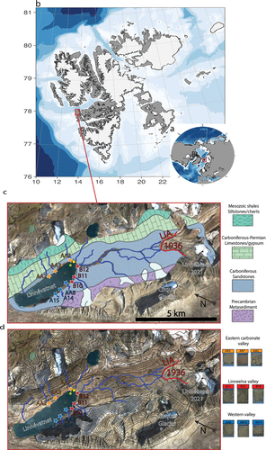
Figure 1. (a) Map of the Northern Hemisphere showing Svalbard location (red rectangle). (b) Map of Svalbard. (c) Zoom of the red rectangle in (b). Stars indicate the location where sediment samples were collected around Linnévatnet. Blue, red, and orange stars are from the western section, Carboniferous quartzites (including main river Linnédalen and the cirque glacier), and the Carboniferous carbonates (eastern portion of the watershed), respectively. The green and the yellow circles are the locations of the 5-m composite sequence at mooring C (this study) and site 06 (Snyder et al. 1994; Svendsen and Mangerud 1997). (a), (b) Maps created with the PlotSvalbard R package (Vihtakari 2019). (c) Satellite high-resolution optical image from Copernicus Sentinel-2 L2A acquired 22 August 2022. The red line is the moraine limit from the LIA. The bedrock geology map (modified from Ohta et al. 1991) contour delimits Linnevatnet’s watershed. The blue lines are the inlets flowing into Linnévatnet. (d) Same as (c) but showing the contour heights of 50 m extracted from G100 Geology shapefiles Svalbard.

Study site

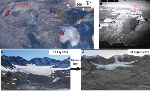
Linnévatnet is a proglacial lake, ~4.7 km long (north–south) and ~1.3 km wide, at 12 m.a.s.l. (Figure 1). A small valley glacier, Linnébreen, though still present in Linnévatnet’s watershed, has retreated steadily since 1936 from its Little Ice Age moraine, when the Norwegian Polar Institute took oblique air photos across the region (Figure 2). The main inflow to Linnévatnet is Linnéelva, a river that flows about 5.5 km from the Little Ice Age moraine to the lake. Two subbasins separated by a submerged ridge define the east and west sections in the southern half of the lake (Snyder, Werner, and Miller 2000). The coring location at mooring C in the eastern basin was chosen for the composite sequence because it is characterized by higher sediment accumulation compared to any other areas of the lake (Svendsen and Mangerud 1997).

Figure 2. (a) Linnébreen ice margin positions since 1936. The positions in 1936 and 1995 are from air photographs and superimposed on georeferenced image from 1995. Positions from 2004 to 2019 are Global Positioning Satellite tracks on georeferenced image. Modified from Retelle et al. (2019). The red line position from 2022 was drawn using the Sentinel-2 L2A image of the ice margin position as observed on 28 August 2022. (b) Aerial photo taken in 1936 showing Linnédalen, courtesy of the Norsk-Polarinstitutt. (c) and (d) Two photos taken in front of Linnébreen at the same position but with ten-year difference.

The principal inflow, Linnéelva, drains the central valley, which is underlain by the coal-bearing plant fossil–rich quartz sandstone of the Lower Carboniferous Orustdalen Formation (Dallmann 2015). The total organic content of Linnévatnet sediments is believed to be largely controlled by Linnéelva carrying ancient fragmental coal, the quantities of which are linked to Linnébreen erosional activity (Svendsen and Mangerud 1997). The second major source is from the eastern flanks of the watershed and consists of carbonates of Upper Carboniferous to Permian age, composed of limestone, dolostone, gypsum, and anhydrite with only a minor amount of coal (Ohta et al. 1992). A third contributing source is from an unnamed ice-free cirque southwest of the lake where a degrading Little Ice Age moraine (Figures 1c and 1d) overlies low-grade metamorphic phyllosilicate minerals from phyllites of the Precambrian Hecla Hoek Formation (Ohta et al. 1992), with negligible other sources of carbonates or coal (Snyder, Werner, and Miller 2000). This bedrock distribution makes Linnévatnet an ideal lake to map these three different sources using high-resolution µ-XRF data.

Methods

Sediment cores and computed tomography scan

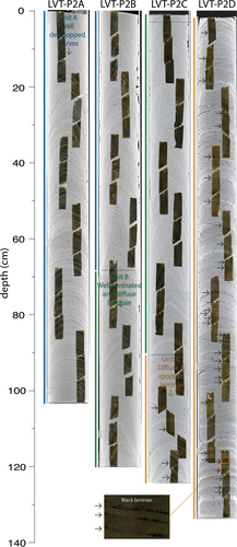
Two sediment cores were collected in April 2019 at mooring C (Figure 1; green circle). They consist of one gravity core (UWITEC core: 41.8 cm) and one 498-cm-long core collected with a piston corer (Nesje 1992). The uppermost sediment from the gravity core was stabilized using floral foam to minimize disturbance of the surface sediment. The long core was a single drive that was sectioned into four parts and labeled as follows: LVT19-P2-A (120.8 cm), LVT19-P2-B (120.4 cm), LVT19-P2-C (124 cm), and LVT-P2-D (133 cm; Figure 3). All of the percussion cores were scanned using computed tomography (CT) at 145 kV, 800 mA for 500 milliseconds with 53 µm voxel size using a ProCon X-ray CT-ALPHA scanner available at the EARTHLAB, University of Bergen. The X-ray beam was filtered through a 0.5-mm Cu filter to reduce beam hardening effects, and data were binned to produce 200-µm resolution 16-bit X-ray imagery. The UWITEC surface core was scanned using CT at 140 kV with 250 mA current at the University of Quebec, Institut National de la Recherche Scientifique. Tomograms of 512 × 512 pixels were acquired continuously at every 0.4 mm along a 0.6-mm-thick slice, allowing for a 0.2-mm overlap between each tomogram. The composite sedimentary record was constructed using the first 41.8 cm of the gravity where a turbidite is stratigraphically matched with LVT19-P2-A at 18-cm depth.

Figure 3. CT scans from the four percussion cores with overlapping thin sections along with the major units found in Linnévatnet sediments at mooring C: Unit A (blue), Unit B (green), and Unit C (orange). Horizontal arrows indicate the presence of distinct black (monosulfidic) laminae. (Bottom) Blowup of a thin section showing black laminae indicative of meromixis conditions.

Thin sections, varve counting

The undisturbed sediments were subsampled using aluminum slabs measuring 7 × 1.5 × 0.7 cm. These samples were then subjected to freeze drying and embedded in epoxy resin (Lamoureux 1994; Francus and Asikainen 2001). Ninety-four overlapping thin sections were made to cover the 5.03-m composite sequence. A homemade software package Analyze Image (Francus and Nobert 2007) was used to store the digitalized thin sections, and regions of interest were then selected and acquired at the scanning electron microscope. About 5,000 backscattered electron (BSE) images were extracted to cover the upper 370 cm of the composite core. These 8-bit grayscale scanning electron microscopy (SEM) images (1,024 × 768 pixels) were obtained with an accelerating voltage of 20 kV and an 8.5 mm working distance with a pixel size of 1 µm. Careful visualization of these BSE images enabled manual definition of varve boundaries (Lapointe et al. 2012).

These BSE images were then transformed into black and white images to measure particle size data at ~1-mm resolution. Each minerogenic particle (with an average of 2,285 per image) was measured for the position of the center of gravity, area, and length of the long and short axes of the best fitting ellipse. Several grain size indices were measured including the median (D₅₀, with D being the apparent disk diameter) and the weight percentage of the following fractions: <16 µm, 16 to 31 µm, 31 to 63 µm, and >63 µm. Weight was calculated using the formula {(4/3) * π * [(D/2)³]} * 2.65 (Figure S1; Francus et al. 2002; Lapointe et al. 2019).

Chronological constraints

Radionuclide ¹³⁷Cs was measured on a sediment core collected in 2016 at mooring C (Williams 2017). Thin sections from this core were visually matched with those collected in our study. Thin sections from cores collected in 2005, 2016, and 2018 were also used to validate the recent chronology. For longer timescales, three radiocarbon dates derived from terrestrial plants in proximal site 06 (Figure 1), a coring site with twice the sedimentation rate compared to mooring C (Snyder et al. 1994), were used to anchor the chronology of the past ~1,500 years. This was done by chemo-stratigraphy between CaCO₃ (percent) from Svendsen and Mangerud (1997) and µ-XRF Ca variations (this study) to locate the ¹⁴C ages from macrofossils at the proximal site and transfer them within the composite depth from our new cores. The uncalibrated ¹⁴C ages were then calibrated using OxCal software with the IntCal20 calibration curve (Ramsey 2008; Reimer et al. 2020). The age model is based on the average varve counts.

Itrax µ-XRF and magnetic susceptibility

An Itrax core scanner with a molybdenum X-ray tube operating at 30kV and 55 mA was used to collect geochemical variations with 200-µm resolution (µ-XRF; Croudace, Rindby, and Rothwell 2006) throughout the ~5-m composite core. These measurements were made with 15 seconds for each step and the counts per second ranged from 18,000 to 24,000. Magnetic susceptibility (MS) was measured with the Itrax-equipped Bartington MS3 magnetic susceptibility meter at 4-mm intervals throughout the 5-m composite sequence.

Fourteen of the twenty-seven surface samples collected around Linnévatnet were also analyzed on the Itrax by constructing an artificial core (Figure 1, colored stars, and Figure S2) using the same settings described above to give insights into sediment provenance variability in the 5-m composite sequence. The µ-XRF data from each site were added into the same data frame and each element was normalized relative to the overall average and standard deviation of each element from all sites combined. Then, the µ-XRF distribution of each individual site was computed. This approach to normalize each individual site to the whole data set provided a better comparison of the relative µ-XRF elemental contributions at the different sampling sites that can be linked to the composite µ-XRF. Note that box plots with original log-µ-XRF values from individual sites (without normalizing using all sites) are provided in Figures S7 to S9.

Density and loss on ignition

A total of 384 discrete surface samples were collected for wet and dry density measurements. Three hundred seventy-seven samples were extracted at a continuous sampling resolution of 1 cm from the composite sequence and seven other samples were collected below 377 cm at 10 cm reaching the 5-m composite. Because of the poor quality of the laminae along with thick turbidites below 370 cm, we decided to focus on the first 370 cm for our study. Prior to weighing the samples, the 384 crucibles were weighed individually and then weighed with the wet sediment. We calculated the wet weight by subtracting the wet sample (inside of the crucible) from the crucible mass. Following drying of sediment at 60°C for two days, the same procedure was applied to measure dry density (sample dry mass minus crucible mass). Afterward, the percentage organics were determined on these samples through loss on ignition (LOI) using a combustion temperature of 550°C for at least four hours (Dean 1974). All of the samples were stored in a desiccator with Drierite to prevent accumulation of moisture. The measurements were made using the same calculation as for the wet and dry density but the percentage organics was calculated by subtracting the sample dry mass from the sample LOI mass. The result was divided by the sample dry mass and then multiplied by 100 to obtain the percentage.

Principal component analysis

Principal component analysis was performed using the FactoMineR and factoextra R packages (Husson et al. 2016; Kassambara and Mundt 2017). The squared cosine (cos²) indicates the importance of each of the µ-XRF elements regarding the principal components; that is, the contribution of an element to the squared distance of the observation to the origin. Cos² was calculated as the contribution of a variable (var) to a given principal component in percentage as (var.cos² * 100)/(total cos² of the principal component). For more information, see Abdi and Williams (2010).

The red dashed line in Figure 8B shows the expected average contribution (percent) of the various elements in principal components (PCs) 1 to 3. If the contributions of each element were uniform, the expected value would be 1/20 (5 percent) for all elements. The contributions of the variable on PC1 and PC2 were calculated as contribution = [(C1 * Eig1) + (C2 * Eig2)]/(Eig1 + Eig2), where C1 and C2 denote the contributions of the µ-XRF on PC1 and PC2, respectively. Eig1 and Eig2 are the eigenvalues of PC1 and PC2, respectively. The expected average contribution of the µ-XRF for PC1 and PC2 is then [(10 * Eig1) + (10 * Eig2)]/(Eig1 + Eig2).

Results

Main sediment units and recent chronology

CT images reveal that the recent sedimentary record contains well-defined laminated sediments (Figure 3). Within the 5 m composite record, three main units can be identified. From the surface to about 170 cm depth, well-defined varves were observed (Unit A: well-developed varves; Figure 3). From ~170 to ~370 cm, laminae were present but less well developed (Unit B: well-laminated and diffuse laminae), and from 370 to 503 cm the facies were characterized by massive sediments sometimes intercalated by diffuse and sporadic laminae (Unit C: diffuse and sporadic laminae). Black laminae were observed in the lowermost part of the composite record, which may reflect anoxic conditions when the lake became isolated from the sea and was density stratified (meromictic conditions; Svendsen and Mangerud 1997). These black laminae decreased in frequency upward to completely disappear at a depth of ~370 cm (Figure 3, arrows). We note that there was no isolation contact defining the transition from sea to lacustrine waters that is visible in the lower part of the composite record.

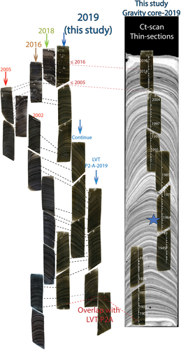
To investigate whether the recent laminae were annually deposited, a sediment core collected in 2016 at mooring C containing a distinctive peak in ¹³⁷Cs was compared to our new 2019 composite record. Stratigraphic matching between laminae from these thin sections (Williams 2017) and those from the gravity core in this study allowed us to interpolate the maximum ¹³⁷Cs peak value to our composite sequence at ~25 cm (Figure 4A; maximum values at ~19 cm for the 2016 core; Figure 4B). This depth is in excellent agreement with the date of 1963 CE obtained with the varve chronology (Figure 4C). Other thin sections from mooring C of sediment cores collected in previous years (2005, 2012, 2016) also enabled us to confirm that the layers were deposited annually (Figure 5).

Figure 4. (a) Thin sections from a core collected in 2016 at mooring C (Williams 2017) compared to the gravity core from this study. (b) ¹³⁷Cs from core collected in 2016 (Williams 2017). (c) Varve chronology from the uppermost 33 cm with the corresponding section where the 1963 (blue) ¹³⁷Cs peak was detected in the core from 2016 as well as the 1952 onset of nuclear testing (red).

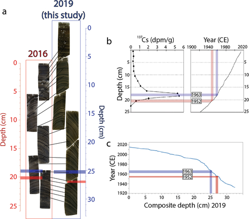
Figure 5. Stratigraphical matching between Linnévatnet thin sections from cores collected in 2019 (this study) and previous years (2018, 2016, and 2005). CT scan of 2019 gravity core with overlapping thin sections. The blue star denotes the location of the ¹³⁷Cs peak (Figure 4). The dense layer located at ~1902 CE was used as a marker for the composite sequence (overlap with percussion core LVT-P2-A-2019).

Clastic facies

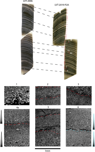
Varve couplets were identified based on the textural properties of the sedimentary layers at Linnévatnet. For the first ~170 cm, couplets were generally easy to distinguish and were characterized by light (coarser) and dark layers (finer) interpreted to represent the melt and winter seasons, respectively (Figures 6 and S3). Stratigraphic comparison between this study’s composite sedimentary record with other thin sections processed from previous samples collected at mooring C revealed a good match. Figure 6 shows an example of two overlapping thin sections made in an earlier study (LVT-2006; Leon 2009) compared with this study (LVT-P2A-2019). Images acquired on the SEM (1 to 6) are examples of layers encountered essentially throughout the first ~170 cm and in most of the first ~370 cm, facies typically found in predominantly clastic Arctic lake settings (Zolitschka et al. 2015). Photograph 1 shows the base of a turbidite composed of coarse sediments that may be the result of intensive snowmelt and/or a large rainfall event, whereas photograph 4 is a typical facies associated with classical snowmelt-dominated years. Photographs 2, 3, and 5 depict varve boundaries that are not easy to delineate without the high-resolution SEM images, as we also found in another annually laminated Arctic lake sediment record (from Sawtooth Lake, Ellesmere Island; Lapointe et al. 2019). These images provide a superior contrast relative to optical images and allow for better delineation of annual couplets. Photograph 6 is typical of thick and successive layers occurring during the same year, which may be the result of several snowmelt and/or rainfall events.

Figure 6. Top: Stratigraphic matching between thin sections from 2006 at mooring C and this study (LVT-P2A; 77.6 to 88.7 cm). Red lines show varve boundaries. Bottom: Scanning electron images of the different lamination/varve found in Linnévatnet. Red lines in the top right image indicate varve boundaries; the blue cyan dashed line in the bottom right image shows an example of a successive layer within one varve year.

Chronology of the last 2,000 years

Using the SEM images of thin sections, we counted around 2,000 couplets on the first ~370 cm of the composite sequence. Three counts were made, which yielded strong consistency between them, especially for the first 170 cm, which contains well-laminated sediments (Figures 7 and S4). From ~170 cm (Unit B: well-laminated and diffuse laminae) and below, the difference in the counts is slightly more pronounced than Unit A (well laminated). Overall, the varve sequence showed that sedimentation rates were quite constant throughout the past ~2,000 years CE, except for higher values between 0 and ~30 CE as well as after the 1980s. The lowest sedimentation rate was found between ~1600 to 1900 CE. For the uppermost ~170 cm or Unit A, around 867 couplets were counted (back to ~1150 CE).

Figure 7. (a) Comparison between µ-XRF Ca (filtered by a 100-point running mean; red) and the carbonates percentage (CaCO₃ percent) from Svendsen and Mangerud (1997). The median calibrated radiocarbon dates are shown and the varve ages corresponding to the depth of radiocarbon ages are in red (mean age of the three varve counts). (b) Age model based on the three counts using SEM images. The blue star indicates the ¹³⁷Cs peak found in our record based on stratigraphical matching with a recent core from Linnévatnet (Figure 4). Also shown are the three calibrated ¹⁴C ages from Snyder et al. (1994) with the ~90 percent probability (green; Figure S4).

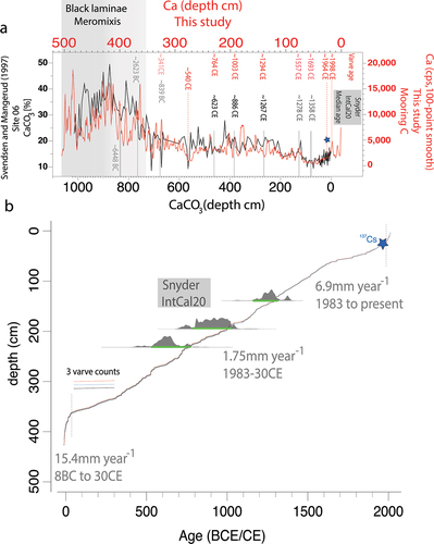
To support the longer timescale chronology, we investigated how the ¹⁴C ages from a previous study compared with our record. This was done by comparing our µ-XRF Ca to the CaCO₃ variations at site 06 (Svendsen and Mangerud 1997), which showed excellent agreement. Based on echosounding, proximal site 06 receives around twice the amount of sediment as mooring C (Svendsen and Mangerud 1997), which is in line with the depth of the stratigraphical matching inferred by the co-variability between CaCO₃ and our µ-XRF Ca. Hence, this allowed us to match the ¹⁴C ages from terrestrial macrofossils (Snyder et al. 1994) to our composite depth. We note that the first two radiocarbon dates appeared too old compared to our chronology. The fact that the third ¹⁴C age was similar to the one at ~1 m above it (the second date) suggests that those two upper dates are indeed unreliable, and these were also discounted in a more recent study focusing on Arctic glacier variability in the context of the Holocene (Paasche and Bakke 2015). The varve counts correlated closely with the youngest side of the ¹⁴C age distribution as seen in Figure 7B, which shows the location of three of these calibrated ¹⁴C ages. Two of three lower ages are within the black laminae zone, suggesting that the lake was recently isolated from the sea with possible seawater intrusions (Svendsen and Mangerud 1997). The one date at median age 839 BC (95 percent probability: 1008–751 BC) is also very close to the disappearance of black laminae and appears too old compared to our chronology (~341 CE).

µ-XRF principal component analysis

The short surface core and the four sediment sections of the longer percussion core are shown in Figure 8c along with variability in calcium (Ca) from the Itrax. As seen in Figures 5 and 8c, the turbidite observed close to the bottom of the gravity core served as a marker to overlap with the first percussion core LVT19-P2-A. Hence, the composite sequence was composed of the gravity core that overlapped with LVT19-P2-A (at 18 cm depth) and the lower sequence was constituted by LVT19-P2-B, -C, and -D. Principal component analysis made on the 5 m composite sequence indicated that Ca contributed the most to the sediment composition at mooring C (Figure 8a).

Figure 8. All µ-XRF elements from the Linnévatnet mooring C sediment composite. (a) Principal component analysis of the eighteen elements. Squared cosine (in color) represents the quality of representation of each of the eighteen µ-XRF data. (b) Contributions (percent) of each element to the first three principal components. The red dashed line delimits the expected average contribution (see Methods). (c) Sediment cores used for the 5.03-m composite sequence showing calcium variability.

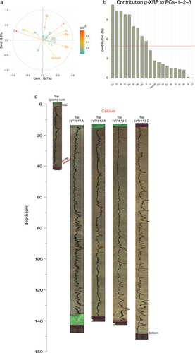
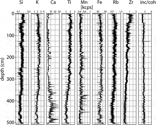
Nine µ-XRF elements were retained as being significant contributors to the three principal components (Ca, Ti, Zr, Fe, Si, Rb, incoherence/coherence ratio [inc/coh], Mn; Figure 8b). PC1 explained 53 percent of the variability, whereas PC2 accounted for ~19 percent (Figure S5). PC1 was associated with Ca, Ti, Rb, Fe, and K, whereas PC2 was linked to Si, inc/coh (associated with water content), and K. Ti and Rb were strongly anticorrelated to Ca variability (Figure 9, Table 1). Fe and K were strongly correlated to Ti; hence, these elements co-varied and appeared to be the main component (53 percent) of sediment delivered to mooring C.

Table 1. Correlation matrix of the nine µ-XRF data for the composite sequence (5.03 m) at 0.2 mm for a total of 25,268 data points.

	Si	K	Ca	Ti	Mn	Fe	Rb	Zr	inc/coh
Si	1
K	0.64	1
Ca	−0.44	−0.64	1
Ti	0.67	0.83	−0.79	1
Mn	−0.01	−0.03	0.31	−0.12	1
Fe	0.37	0.78	−0.60	0.55	−0.03	1
Rb	0.45	0.74	−0.75	0.79	−0.17	0.61	1
Zr	0.63	0.45	−0.61	0.76	−0.11	0.11	0.52	1
inc/coh	−0.40	−0.12	−0.08	−0.27	−0.21	0.22	−0.03	−0.50	1

Note. Bold values indicate significance at p < .001.

Figure 9. µ-XRF variations for the composite sequence at mooring (Figures 1c, 1d; green circle) for the first 5 m. Results are expressed in thousand counts per second (kcps) for silicon (Si), potassium (K), calcium (Ca), titanium (Ti), manganese (Mn), iron (Fe), rubidium (Rb), zirconium (Zr), and the incoherence/coherence ratio (inc/coh).

LOI, grain size, and elemental variations

Ca is inversely correlated to organic content (Figure 10a) and positively correlated to the MS measurements (Figure S6). Organic content and MS were strongly and negatively correlated throughout the uppermost 370 cm (Figure 10b; r = −0.55, p < .001: resampled at 1 cm). Higher MS was observed in the deeper part of the record, followed by a sharp decrease around 460 cm, coinciding with some of the lowest MS values of the whole ~5-m composite between ~460 and 370 cm depth (Figure S6). Thin sections also revealed that below ~370 cm the sediment was more compact and intercalated with diffuse and thick laminae (Figure 3: Unit C) with random increases in Ca as well as the presence of black laminae (Figure 3). This is a feature also shown in the CaCO₃, implying a sharp increase in sedimentation rate during this interval. For this reason, grain size as well as absolute density measurements and LOI were only continuously collected for the upper ~370 cm.

Figure 10. Organics (percent) compared with (a) Ca resampled at 1 cm and (b) MS. (c) D₅₀ (µm), resampled at 1 cm, compared with calcium of the first 370 cm of the composite sequence. Correlations in gray are for the first 170 cm.

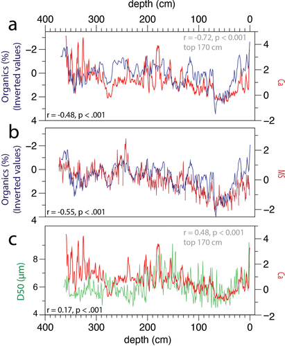
A positive correlation was also found between grain size (D₅₀) and Ca (Figure 10c; r = 0.18, p < .001), and this relationship increased sharply in the upper ~170 cm of the composite sequence (r = 0.47, p < .001). This was also the case with the Ca and organics (r = −0.72, p < .001; Figure 10a).

Sediment samples collected in the watershed and their potential source inferred from µ-XRF

To link sediment provenance to the composite µ-XRF, samples collected in areas with different lithologies were analyzed for their µ-XRF content: (1) the eastern carbonate valley wall, (2) Linnéelva river delta, (3) the cirque glacier fan delta, and (4) the wider eastern valley area. Nine sediment samples were processed on the Itrax (see methods; Figure 1, colored stars).

Samples from the eastern valley (composed of carbonates) were the most enriched in Ca (Figure 11a), whereas all other sites showed negative Ca values. Greater Zr and Ti values as well as positive Si anomalies at the Linnéelva delta (Figure 11b: B12) are indicative of quartzitic sandstone. In the watershed, the sandstone was most prevalent in sediment underlying Linnébreen glacier and Linnéelva (Potter 2017). Positive Ti values were mainly found in the samples collected at the Linnéelva delta and the meltwater fan from the cirque glacier (Figure 11: B10, B12).

Figure 11. Box plots of the samples shown in Figures 1c and 1d with their µ-XRF anomalies. (a) The Eastern valley wall (AA2, AA7, and AA3). (b) The outlet of the main river Linnéelva (B12), as well as B11 and B10 (the outlet of the cirque glacier). (c) Location of the samples for the West valley (AA8, AA14, and AA15).

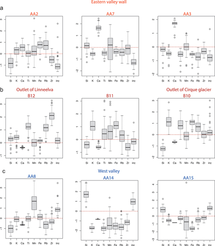
Samples B11 and B10 and, to a lesser extent, AA2 were characterized by positive K anomalies compared to all other samples. Sediment from the cirque alluvial fan had lesser amounts of carbonate, and only trace amounts of coal were present (Snyder, Werner, and Miller 2000). The sample collected at the cirque moraine (Figure 1) yielded results similar to B10. Hence, the presence of Precambrian phyllites in this area (Ohta et al. 1991) is consistent with positive K values (Figure 11b; B10). Because of the scarcity of the two principal sources of sediment types in Linnévatnet in the western valley—that is, carbonates and coal (Snyder, Werner, and Miller 2000)—µ-XRF K has great potential to track changes in glacial activity inferred from the cirque glacier through time. We note that µ-XRF data should be taken cautiously because they are sensitive to grain size and water content changes (Croudace, Rindby, and Rothwell 2006), making these data somewhat qualitative; however, positive Ca anomalies were only found in the eastern valley, and thus we assume that its increase in the µ-XRF composite was principally from that area. D₅₀ is highly correlated with the coarse silt fraction (Figure S1: percentage 31–63 µm) and so an increase in Ca from the eastern valley is generally associated with coarser grain size deposits at the coring site.

Discussion

Previous studies have suggested that the contribution of coal exhibits a first-order control on the sedimentation in Linnévatnet (Svendsen and Mangerud 1997; Van Exem et al. 2019). This is because Linnébreen is underlain by coal-bearing sandstones, and it is thought that the growth of the glacier would result in increased subglacial erosion of the Carboniferous coal and subsequent transport by Linnéelva to the lake. As a result, total organic carbon deposited in Linnévatnet has been used as a proxy to monitor periods of higher glacial activity. Results shown here suggest that Ca and organics (percent, from coal) are intrinsically linked; that is, when one increases the other decreases and vice versa. These findings are in line with previous analysis of Linnévatnet sedimentary records using a much coarser sampling resolution (Svendsen and Mangerud 1997).

The strong negative correlation between Ca and organic content (percent) suggests that the overall sediment load consisted of an alternation of the coal-rich sandstone found in the central portion of Linnédalen and the eastern valley carbonates. These observations indicate that the main sediment supply to mooring C and the eastern proximal basin comes from either the main river (Linnéelva) and the cirque glacier or the carbonate alluvial fans from the eastern valley (Figures 8 and 9). More recently, Ca (and grain size values) has increased steadily from 50 cm to the top of the sedimentary record, whereas Si, Zr, and K values all declined (Figure 9). This is a strong indication that the sediment input from the carbonate alluvial fans has become the dominant source of sediment delivery at mooring C in recent history. As precipitation in the form of rain is rising (whereas snowfall is decreasing) in much of Svalbard (Nowak et al. 2021), the sediment flux is more pronounced in the eastern flanks of the valley because the slopes are much steeper compared to the central flat valley (Figure 1c), resulting in a steady increase in Ca and grain size over recent decades.

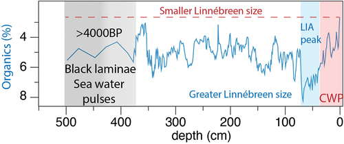
The ongoing retreat and thinning of Linnébreen (Figure 2) since the end of the Little Ice Age has caused a decrease in sediment derived from glacial abrasion and a relative increase in sediment from paraglacial and periglacial sources (Church and Ryder 1972; Leonard 1997; Ballantyne 2002). Percentage organics was also at the lowest concentrations in the uppermost 20 cm (Figure 12), which is also diagnostic of the decreasing influence of Linnébreen’s abrasion of coal-bearing sandstone and subsequent transport into the lake. The presence of black laminae, likely associated with the isolation of the lake from the sea, along with massive sediment and sporadic laminae in the lowermost part of the composite record indicates that the age of the lower record is likely to be older than ~4,000 years BP (Svendsen and Mangerud 1997). Based on the varve chronology, our results thus suggest that the Linnébreen’s influence on the lake sediment influx is at an all-time low in the context of the past several millennia (Figure 12).

Figure 12. Loss on ignition (organics percent) throughout the first 5 m of the composite sequence. Increased (decreased) organics (percent) reflects greater (lower) influence of Linnébreen erosion on the sedimentary record. CWP and LIA peak denote the current warm period and Little Ice Age peak.

Correlation with instrumental data

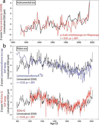
Because the varve chronology was robust (Figure 7), this allowed us to compare our annually resolved grain size (D₅₀) to seasonal temperature and precipitation from Longyearbyen covering the last ~100 years (Ø. Nordli et al. 2014). Seasonal temperatures (DJF, MAM, JJA, SON) were all significantly correlated to D₅₀, whereas seasonal precipitation was only significantly correlated during summer and fall. We note that temperature and precipitation were more strongly correlated with D₅₀ during summer and fall than other seasons.

These findings suggest that temperature and precipitation interact to amplify the grain size signal in the sedimentary record. This was supported by multiple linear regression between annual D₅₀ and the two independent variables (temperature and precipitation) showing a stronger correlation (r = 0.61, p < .001) than taken individually (Table 2). Significant correlations are also found with Ca (Ca and JJASON temperature and precipitation: r = 0.37 and 0.40, respectively). To give a sense of this relationship, we used the time series based on the multiple regression equation and compared it to D₅₀ at Linnévatnet from 2017 to 1912 (Figure 13a). The significant correlation implies that the D₅₀ record can be used as a hydroclimate proxy for the past several centuries.

Table 2. (A) Annual coarse grain size at Linnévatnet correlated to seasonal temperature at Longyearbyen 1898 to 2017 (Ø. Nordli et al. 2014). (B) Grain size at Linnévatnet correlated to seasonal precipitation at Longyearbyen from 1912 to 2017 (Ø. Nordli, Hanssen-Bauer, and Førland 1996).

	D50	DJF	MAM	JJA	SON
(A)
D50	1
DJF	0.4	1
MAM	0.33	0.53	1
JJA	0.42	0.58	0.48	1
SON	0.5	0.65	0.48	0.56	1
(B)
D50	1
DJF	0.21	1
MAM	−0.04	0.01	1
JJA	0.22	0.07	−0.017	1
SON	0.39	0.18	0.05	0.27	1

Note. Bold numbers indicate significant correlation (p < .01).

Figure 13. (a) Normalized Linnévatnet D₅₀ (µm) compared with the sum of Z-score temperature and precipitation during June to November (JJASON); a three-year running mean was applied on the D₅₀ time series. (b) D₅₀ (µm) is compared with δ¹⁸O from Lomonosovsfonna (DJF temperature) in Svalbard. Same as upper panel, but Linnévatnet D₅₀ (µm) is compared to normalized December to February temperature from climate model Echo-G. D₅₀ is filtered by an eleven-year running mean in (b).

Comparison with other regional and hemispherical records

There are few subdecadal records in Svalbard to compare with our record; however, Lomonovsfonna δ¹⁸O, an ice core record (located ~114 km northeast from Linnévatnet), revealed a strong co-variability with the Linnévatnet D₅₀ record (r = 032, p < .001; annual) as well as Ca (Figure S10). This ice core record tracks winter temperature variability (Divine et al. 2011), and although D₅₀ was better correlated to summer and fall temperature, each season was significantly correlated to each other, so a significant correlation of D₅₀ with Lomonovsfonna δ¹⁸O can be expected (Figure 13b).

Our annually resolved grain size also bears striking co-variability with the Northern Hemisphere winter temperature from the Echo-G model simulation (r = 0.43, p < .001; annual) that combines solar, volcanic, and greenhouse gas variations; that is, external forcing (Osborn, Raper, and Briffa 2006). Spatial correlations between Echo-G temperature and sea surface temperature (SST: Huang et al. 2017) as well as D₅₀ and SST depicted a similar pattern of warmer SSTs centered around Svalbard and in other regions (Figure S11). A warmer ocean leads to more moisture availability, which creates favorable conditions for summer and fall rain events to occur, consistent with multiple linear regression and the observed increasing trend in the last ~100 years (Figure 13a). A notable feature of the reconstructions is the relatively warm period around 1100 to 1200 CE seen in the Svalbard proxies (Linnévatnet and Lomonosovfonna) as well as the Northern Hemisphere temperature simulation. Remarkably, the late 1140s (peaking at 1147 CE) appeared as the warmest period during the Medieval Climate Anomaly, which was highlighted by Divine et al. (2011) as being one of the warmest periods, up to and including the 1990s. In this regard, our more recent sedimentary record suggests that the temperature of the past few years now exceeds that of the warmest interval in Medieval times, which is also consistent with the unprecedented shrinking of Linnébreen glacier (Figures 2, 12, and 14c).

Figure 14. (a), (b), (c) Calcium, grain size D₅₀ (µm), June to November temperature at the Svalbard airport from 1898 to 2022, and percentage organics variability extracted from the composite sequence at mooring C (Figures 1c, 1d: green circle). Vertical dashed lines indicate timing of sudden shifts in the record that may potentially be associated with the abrupt cooling documented following the eruption of an unknown volcano (536 CE), as well as the eruption of the Samalas volcano (1257 CE). The chronology being analyzed encompasses a period of ~2,000 years.

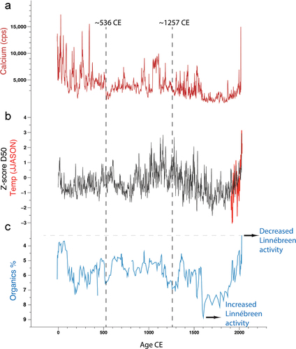
It is likely that the strong declining trend in the grain size data is related to the millennial cooling trend in temperature. Of note is the abrupt transition toward cooler conditions that occurred in the 1570s, as seen in the sedimentary record (Ca, LOI, and D₅₀), with lowest values in the 1600s that persisted until the early 1800s. These observations are in line with reconstructed sea-ice extent of the Western Nordic Seas showing highest values occurring at the turn of the seventeenth century that persisted until the nineteenth century (Macias Fauria et al. 2010). Climate simulations and historical evidence suggest a strong cooling of the northern North Atlantic following the Huaynaputina eruption in 1600 CE, triggering persistent sea ice year-round (White et al. 2022). This period coincided with the coolest Atlantic SSTs (Lapointe et al. 2020) as well as a weaker subpolar gyre shortly after 1600 CE (Moreno-Chamarro et al. 2017; Lapointe and Bradley 2021). As summers became cooler, it is plausible that Linnébreen increased in size as a result of less ablation and increased precipitation in the form of snow. The sharp increase in organics at this time (and concomitant decrease in Ca and D₅₀) supports the hypothesis of a regrowth of Linnébreen in the early 1600s that resulted in finer particle size deposition in Linnévatnet (Figure 14). Meanwhile, the depleted Ca input to the lake is indicative of inactive eastern carbonate alluvial fans. In West Greenland and Baffin Island, glacial advances around ~1570 CE were also documented (Young et al. 2015; Jomelli et al. 2016). There was also an increase in organics between 1200 and 1300 CE, which was similarly documented at Linnévatnet by Svendsen and Mangerud (1997). Ca values decreased after ~1257 CE (and organics increased further), which may be related to a significant climatic effect of the largest volcanic eruption of the past millennium (the 1257 CE Samalas eruption in Indonesia). In summary, our paleoclimatological investigation suggests that Svalbard is sensitive to external forcing and tracks large-scale climatic variability over the past thousand years.

Prior to the last millennium, a decreasing trend in the organics suggests ice retreat of Linnébreen starting at ~300 CE and culminating at ~500 CE, although independent dating is needed to confirm this chronology. Nevertheless, our results agree well with ¹⁰Be exposure ages on moraine boulders from Linnébreen and other glaciers from Spitsbergen’s west coast (Reusche et al. 2014; Philipps et al. 2017; Farnsworth et al. 2020). During that time, an increased presence of warm Atlantic waters was recorded around Svalbard, coinciding with the “Roman Warm period” (Reusche et al. 2014; Lapointe et al. 2020). Linnébreen ice growth increased in the late 530s, as reflected by increasing organic input (Figure 14). This was also reflected by lower calcium values and, to a lesser extent, in the grain size data. The timing matches with the well-known (and unnamed) large eruption dated 536 CE (Sigl et al. 2015; Büntgen et al. 2016), suggesting that, overall, the varve record seems to be quite sensitive to volcanic forcing. The ongoing warming and hydroclimatic change in Svalbard of the past few years is outside the natural range of variability during the past millennium (Figures 13 and 14). Based on meteorological inferences (Table 2), this recent hydrological shift is characterized by an increase in rain during summer and fall as inferred from the abrupt increase in grain size and Ca. Finally, the lowest organic content occurred in recent years, highlighting that the current warming appears unmatched during the past millennia.

Conclusions

Sediment samples collected around Linnévatnet enabled the identification of three sources of sediment delivery to mooring C: the carbonate-rich alluvial fan on the eastern basin, the coal-bearing sandstones from the central valley, and the phyllite sediments from the cirque glacier area. The principal source for sediment delivery at mooring C is Ca, and the fact that Ca, MS, and organics (percent) are all interrelated support previous interpretations that Ca and organic content are inversely correlated and may serve as proxies for warmer and wetter (higher Ca) versus cooler (higher organics) conditions. As previously shown (Svendsen and Mangerud 1997), organics (percent) can thus be used to reconstruct the relative influence of Linnnébreen on the lake sedimentation. The results reveal an ongoing retreat of Linnébreen glacier since the end of the Little Ice Age coinciding with increasing grain size and Ca. Importantly, Linnébreen’s deterioration over the past decade is unprecedented in the context of the past several millennia, and the warming in Svalbard has now exceeded that in Medieval times, consistent with the recent reappearance of blue mussels (Mytilus edulis) in Svalbard after an ~1,000-year absence (Berge et al. 2005). Finally, precipitation in the form of rain has risen considerably in Svalbard in recent years (Nowak et al. 2021), and this hydrological shift will likely become prevalent with the ongoing warming trend.

Acknowledgments

We thank Astrid Vikingstad for the CaCO₃ data set and notes. We are grateful for comments by John Inge Svendsen.

Disclosure statement

No potential conflict of interest was reported by the authors.

Supplementary material

Supplemental data for this article can be accessed online at https://doi.org/10.1080/15230430.2023.2223403.

Additional information

Funding

This work was supported by the U.S. National Science Foundation (Grant No. 1744515).

References

- Abdi, H., and L. J. Williams. 2010. Principal component analysis. Wiley Interdisciplinary Reviews: Computational Statistics 2, no. 4: 433–22. doi:10.1002/wics.101.
- Bakke, J., N. Balascio, W. G. van der Bilt, R. Bradley, W. J. D’Andrea, M. Gjerde, S. Ólafsdóttir, T. Røthe, and G. De Wet. 2018. The Island of Amsterdamøya: A key site for studying past climate in the Arctic archipelago of Svalbard. Quaternary Science Reviews 183: 157–63. doi:10.1016/j.quascirev.2017.11.005.
- Balascio, N. L., W. J. D’Andrea, M. Gjerde, and J. Bakke. 2018. Hydroclimate variability of High Arctic Svalbard during the Holocene inferred from hydrogen isotopes of leaf waxes. Quaternary Science Reviews 183: 177–87. doi:10.1016/j.quascirev.2016.11.036.
- Ballantyne, C. K. 2002. Paraglacial geomorphology. Quaternary Science Reviews 21: 1935–2017.
- Berge, J., G. Johnsen, F. Nilsen, B. Gulliksen, and D. Slagstad. 2005. Ocean temperature oscillations enable reappearance of blue mussels Mytilus edulis in Svalbard after a 1000 year absence. Marine Ecology Progress Series 303: 167–75. doi:10.3354/meps303167.
- Büntgen, U., V. S. Myglan, F. C. Ljungqvist, M. McCormick, N. Di Cosmo, M. Sigl, J. Jungclaus, S. Wagner, P. J. Krusic, and J. Esper. 2016. Cooling and societal change during the late antique Little Ice Age from 536 to around 660 AD. Nature Geoscience 9: 231–6. doi:10.1038/ngeo2652.
- Church, M., and J. M. Ryder. 1972. Paraglacial sedimentation: A consideration of fluvial processes conditioned by glaciation. Geological Society of America Bulletin 83, no. 10: 3059–72. doi:10.1130/0016-7606(1972)83[3059:PSACOF]2.0.CO;2.
- Croudace, I. W., A. Rindby, and R. G. Rothwell. 2006. ITRAX: Description and evaluation of a new multi-function X-ray core scanner. Special Publication-Geological Society of London 267, no. 1: 51. doi:10.1144/GSL.SP.2006.267.01.04.
- Dallmann, W. K. 2015. Geoscience Atlas of Svalbard. Norsk Polarinstitutt Rapportserie 148: 1e292.
- Dean, W. E. 1974. Determination of carbonate and organic matter in calcareous sediments and sedimentary rocks by loss on ignition; comparison with other methods. Journal of Sedimentary Research 44: 242–8.
- Divine, D., E. Isaksson, T. Martma, H. A. J. Meijer, J. Moore, V. Pohjola, R. S. W. van de Wal, and F. Godtliebsen. 2011. Thousand years of winter surface air temperature variations in Svalbard and northern Norway reconstructed from ice-core data. Polar Research 30, no. 1: 7379. doi:10.3402/polar.v30i0.7379.
- Eckerstorfer, M., and H. H. Christiansen. 2011. The “High Arctic maritime snow climate” in central Svalbard. Arctic, Antarctic, and Alpine Research 43, no. 1: 11–21. doi:10.1657/1938-4246-43.1.11.
- Farnsworth, W. R., L. Allaart, Ó. Ingólfsson, H. Alexanderson, M. Forwick, R. Noormets, M. Retelle, and A. Schomacker. 2020. Holocene glacial history of Svalbard: Status, perspectives and challenges. Earth-Science Reviews 208: 103249. doi:10.1016/j.earscirev.2020.103249.
- Francus, P., and C. A. Asikainen. 2001. Sub-sampling unconsolidated sediments: A solution for the preparation of undistrubed thin-sections from clay-rich sediments. Journal of Paleolimnology 26, no. 3: 323–6. doi:10.1023/A:1017572602692.
- Francus, P., R. S. Bradley, M. B. Abbott, W. Patridge, and F. Keimig. 2002. Paleoclimate studies of minerogenic sediments using annually resolved textural parameters. Geophysical Research Letters 29, no. 20: 59-1–59–4. doi:10.1029/2002GL015082.
- Francus, P., and P. Nobert. 2007. An integrated computer system to acquire, process, measure and store images of laminated sediments. 4th International Limnogeology Congress, July 11–14, Barcelona.
- Geyman, E. C., W. Jj van Pelt, A. C. Maloof, H. F. Aas, and J. Kohler. 2022. Historical glacier change on Svalbard predicts doubling of mass loss by 2100. Nature 601, no. 7893: 374–9. doi:10.1038/s41586-021-04314-4.
- Hald, M., C. Andersson, H. Ebbesen, E. Jansen, D. Klitgaard-Kristensen, B. Risebrobakken, G. R. Salomonsen, M. Sarnthein, H. P. Sejrup, and R. J. Telford. 2007. Variations in temperature and extent of Atlantic water in the northern North Atlantic during the Holocene. Quaternary Science Reviews 26, no. 25–28: 3423–40. doi:10.1016/j.quascirev.2007.10.005.
- Hetzinger, S., J. Halfar, Z. Zajacz, and M. Wisshak. 2019. Early start of 20th-century Arctic sea-ice decline recorded in Svalbard coralline algae. Geology 47, no. 10: 963–7. doi:10.1130/G46507.1.
- Hole, G. M., T. Rawson, W. R. Farnsworth, A. Schomacker, Ó. Ingólfsson, and M. Macias‐Fauria. 2021. A driftwood‐based record of Arctic sea ice during the last 500 years from northern Svalbard reveals sea ice dynamics in the Arctic Ocean and Arctic peripheral seas. Journal of Geophysical Research: Oceans 126: e2021JC017563.
- Huang, B., P. W. Thorne, V. F. Banzon, T. Boyer, G. Chepurin, J. H. Lawrimore, M. J. Menne, T. M. Smith, R. S. Vose, and H.-M. Zhang. 2017. Extended reconstructed sea surface temperature, version 5 (ERSSTv5): Upgrades, validations, and intercomparisons. Journal of Climate 30, no. 20: 8179–205. doi:10.1175/JCLI-D-16-0836.1.
- Husson, F., J. Josse, S. Le, J. Mazet, and M. F. Husson. 2016. Package ‘factominer. An R Package 96: 698.
- Isaksson, E., J. Kohler, V. Pohjola, J. Moore, M. Igarashi, L. Karlöf, T. Martma, H. Meijer, H. Motoyama, and R. Vaikmäe. 2005. Two ice-core δ18O records from Svalbard illustrating climate and sea-ice variability over the last 400 years. The Holocene 15, no. 4: 501–9. doi:10.1191/0959683605hl820rp.
- Jomelli, V., T. Lane, V. Favier, V. Masson-Delmotte, D. Swingedouw, V. Rinterknecht, I. Schimmelpfennig, D. Brunstein, D. Verfaillie, and K. Adamson. 2016. Paradoxical cold conditions during the medieval climate anomaly in the Western Arctic. Scientific Reports 6, no. 1: 1–9. doi:10.1038/srep32984.
- Kassambara, A., and F. Mundt. 2017. Package ‘factoextra.’ Extract and visualize the results of multivariate data analyses. Accessed 30 August 2022. https://github.com/kassambara/factoextra.
- Kjellman, S. E., A. Schomacker, E. K. Thomas, L. Håkansson, S. Duboscq, A. A. Cluett, W. R. Farnsworth, L. Allaart, O. C. Cowling, and N. P. McKay. 2020. Holocene precipitation seasonality in northern Svalbard: Influence of sea ice and regional ocean surface conditions. Quaternary Science Reviews 240: 106388. doi:10.1016/j.quascirev.2020.106388.
- Lamoureux, S. F. 1994. Embedding unfrozen lake sediments for thin section preparation. Journal of Paleolimnology 10, no. 2: 141–6. doi:10.1007/BF00682510.
- Lapointe, F., and R. S. Bradley. 2021. Little Ice Age abruptly triggered by intrusion of Atlantic waters into the Nordic Seas. Science Advances 7, no. 51: eabi8230. doi:10.1126/sciadv.abi8230.
- Lapointe, F., R. S. Bradley, P. Francus, N. L. Balascio, M. B. Abbott, J. S. Stoner, G. St-Onge, A. De Coninck, and T. Labarre. 2020. Annually resolved Atlantic sea surface temperature variability over the past 2,900 y. Proceedings of the National Academy of Sciences 117, no. 44: 27171–8. doi:10.1073/pnas.2014166117.
- Lapointe, F., P. Francus, S. F. Lamoureux, M. Saïd, and S. Cuven. 2012. 1750 years of large rainfall events inferred from particle size at East Lake, Cape Bounty, Melville Island, Canada. Journal of Paleolimnology 48, no. 1: 159–73. doi:10.1007/s10933-012-9611-8.
- Lapointe, F., P. Francus, J. S. Stoner, M. B. Abbott, N. L. Balascio, T. L. Cook, R. S. Bradley, S. L. Forman, M. Besonen, and G. St-Onge. 2019. Chronology and sedimentology of a new 2.9 ka annually laminated record from South Sawtooth Lake, Ellesmere Island. Quaternary Science Reviews 222: 105875. doi:10.1016/j.quascirev.2019.105875.
- Leon, B. 2009. Comparison of lamination stratigraphies of cores recovered from the proximal basin of Lake Linne, Svalbard, Norway. Mount Holyoke College. https://scarab.bates.edu/geology_theses/35/.
- Leonard, E. M. 1997. The relationship between glacial activity and sediment production: Evidence from a 4450-year varve record of neoglacial sedimentation in Hector Lake, Alberta, Canada. Journal of Paleolimnology 17, no. 3: 319–30. doi:10.1023/A:1007948327654.
- Macias Fauria, M., A. Grinsted, S. Helama, J. Moore, M. Timonen, T. Martma, E. Isaksson, and M. Eronen. 2010. Unprecedented low twentieth century winter sea ice extent in the Western Nordic Seas since AD 1200. Climate Dynamics 34, no. 6: 781–95. doi:10.1007/s00382-009-0610-z.
- Moreno-Chamarro, E., D. Zanchettin, K. Lohmann, and J. H. Jungclaus. 2017. An abrupt weakening of the subpolar gyre as trigger of Little Ice Age-type episodes. Climate Dynamics 48, no. 3–4: 727–44. doi:10.1007/s00382-016-3106-7.
- Nesje, A. 1992. A piston corer for lacustrine and marine sediments. Arctic and Alpine Research 24, no. 3: 257–9. doi:10.2307/1551667.
- Nilsen, F., F. Cottier, R. Skogseth, and S. Mattsson. 2008. Fjord–shelf exchanges controlled by ice and brine production: The interannual variation of Atlantic Water in Isfjorden, Svalbard. Continental Shelf Research 28, no. 14: 1838–53. doi:10.1016/j.csr.2008.04.015.
- Nordli, P. Ø., I. Hanssen-Bauer, and E. Førland. 1996. Homogeneity analyses of temperature and precipitation series from Svalbard and Jan Mayen (DNMI-KLIMA report 16/96). Oslo: Norwegian Meteorological Institute.
- Nordli, Ø., R. Przybylak, A. E. Ogilvie, and K. Isaksen. 2014. Long-term temperature trends and variability on Spitsbergen: The extended Svalbard Airport temperature series, 1898–2012. Polar Research 33, no. 1: 21349. doi:10.3402/polar.v33.21349.
- Nowak, A., R. Hodgkins, A. Nikulina, M. Osuch, T. Wawrzyniak, J. Kavan, E. Łepkowska, M. Majerska, K. Romashova, and I. Vasilevich. 2021 . From land to fjords: The review of Svalbard hydrology from 1970 to 2019. State of Environmental Science in Svalbard (SESS) report 2020. https://sios-svalbard.org/SESS_Issue3.
- Nowak, A., and A. Hodson. 2013. Hydrological response of a High-Arctic catchment to changing climate over the past 35 years: A case study of Bayelva watershed, Svalbard. Polar Research 32, no. 1: 19691. doi:10.3402/polar.v32i0.19691.
- Ohta, Y., A. Hjelle, A. Andresen, W. Dallmann, and O. Salvigsen. 1992. Geological map of Svalbard, 1: 100,000, sheet B9G, Isfjorden. Norsk Polarinstitutt Temakart. 16. Norwegian Polar Institute Oslo.
- Ohta, Y., A. Hjelle, A. Andresen, W. Dallmann, and O. Sålvigsen. 1991. Geological map of Svalbard, 1: 100 000. Sheet B9G Isfjorden, with description. Norsk Polarinstitutt Temakart. 16.
- Osborn, T. J., S. C. Raper, and K. R. Briffa. 2006. Simulated climate change during the last 1,000 years: Comparing the ECHO-G general circulation model with the MAGICC simple climate model. Climate Dynamics 27, no. 2–3: 185–97. doi:10.1007/s00382-006-0129-5.
- Paasche, Ø., and J. Bakke. 2015. The fleeting glaciers of the Arctic. In The New Arctic, eds. B. Evengård, J. N. Larsen, and Ø. Paasche. Cham: Springer, 79–93.
- Peral, M., W. E. Austin, and R. Noormets. 2022. Identification of Atlantic water inflow on the north Svalbard shelf during the Holocene. Journal of Quaternary Science 37, no. 1: 86–99. doi:10.1002/jqs.3374.
- Philipps, W., J. Briner, L. Gislefoss, H. Linge, T. Koffman, D. Fabel, S. Xu, and A. Hormes. 2017. Late Holocene glacier activity at inner Hornsund and Scottbreen, southern Svalbard. Journal of Quaternary Science 32, no. 4: 501–15. doi:10.1002/jqs.2944.
- Potter, N. L. 2017. Late-season high-sedimentation events in a sediment trap record from Linnévatnet, Svalbard, Norway. Standard Theses 31. Bates College.
- Ramsey, C. B. 2008. Deposition models for chronological records. Quaternary Science Reviews 27, no. 1–2: 42–60. doi:10.1016/j.quascirev.2007.01.019.
- Rasmussen, T. L., M. Forwick, and A. Mackensen. 2012. Reconstruction of inflow of Atlantic Water to Isfjorden, Svalbard during the Holocene: Correlation to climate and seasonality. Marine Micropaleontology 94: 80–90. doi:10.1016/j.marmicro.2012.06.008.
- Reimer, P. J., W. E. Austin, E. Bard, A. Bayliss, P. G. Blackwell, C. B. Ramsey, M. Butzin, H. Cheng, R. L. Edwards, and M. Friedrich. 2020. The IntCal20 Northern Hemisphere radiocarbon age calibration curve (0–55 cal kBP). Radiocarbon 62, no. 4: 725–57. doi:10.1017/RDC.2020.41.
- Retelle, M., H. Christiansen, A. Hodson, A. Nikulina, M. Osuch, K. Poleshuk, K. Romashova, S. Roof, L. Rouyet, and S. M. Strand. 2019. Environmental monitoring in the Kapp Linne-Gronfjorden Region (KLEO). https://sios-svalbard.org/sites/sios-svalbard.org/files/common/SESS_2019_03_KLEO.pdf.
- Reusche, M., K. Winsor, A. E. Carlson, S. A. Marcott, D. H. Rood, A. Novak, S. Roof, M. Retelle, A. Werner, and M. Caffee. 2014. 10Be surface exposure ages on the late-Pleistocene and Holocene history of Linnébreen on Svalbard. Quaternary Science Reviews 89: 5–12. doi:10.1016/j.quascirev.2014.01.017.
- Schiefer, E., D. Kaufman, N. McKay, M. Retelle, A. Werner, and S. Roof. 2018. Fluvial suspended sediment yields over hours to millennia in the High Arctic at proglacial Lake Linnévatnet, Svalbard. Earth Surface Processes and Landforms 43, no. 2: 482–98. doi:10.1002/esp.4264.
- Sigl, M., M. Winstrup, J. R. McConnell, K. C. Welten, G. Plunkett, F. Ludlow, U. Büntgen, M. Caffee, N. Chellman, and D. Dahl-Jensen. 2015. Timing and climate forcing of volcanic eruptions for the past 2,500 years. Nature 523, no. 7562: 543–9. doi:10.1038/nature14565.
- Skirbekk, K., D. K. Kristensen, T. L. Rasmussen, N. Koç, and M. Forwick. 2010. Holocene climate variations at the entrance to a warm Arctic fjord: Evidence from Kongsfjorden trough, Svalbard. Geological Society, London, Special Publications 344, no. 1: 289–304. doi:10.1144/SP344.20.
- Ślubowska-Woldengen, M., T. L. Rasmussen, N. Koç, D. Klitgaard-Kristensen, F. Nilsen, and A. Solheim. 2007. Advection of Atlantic water to the western and northern Svalbard shelf since 17,500 cal yr BP. Quaternary Science Reviews 26, no. 3–4: 463–78. doi:10.1016/j.quascirev.2006.09.009.
- Snyder, J., G. Miller, A. Werner, A. Jull, and T. Stafford Jr. 1994. AMS-radiocarbon dating of organic-poor lake sediment, an example from Linnévatnet, Spitsbergen, Svalbard. The Holocene 4, no. 4: 413–21. doi:10.1177/095968369400400409.
- Snyder, J., A. Werner, and G. Miller. 2000. Holocene cirque glacier activity in western Spitsbergen, Svalbard: Sediment records from proglacial Linnévatnet. The Holocene 10, no. 5: 555–63. doi:10.1191/095968300667351697.
- Svendsen, J. I., and J. Mangerud. 1997. Holocene glacial and climatic variations on Spitsbergen, Svalbard. The Holocene 7, no. 1: 45–57. doi:10.1177/095968369700700105.
- van Exem, A., M. Debret, Y. Copard, C. Verpoorter, G. De Wet, N. Lecoq, P. Sorrel, A. Werner, S. Roof, and B. Laignel. 2019. New source-to-sink approach in an Arctic catchment based on hyperspectral core-logging (Lake Linné, Svalbard). Quaternary Science Reviews 203: 128–40. doi:10.1016/j.quascirev.2018.10.038.
- Vihtakari, M. 2019. PlotSvalbard: PlotSvalbard-Plot research data from Svalbard on maps. R package version 0.8 5.
- Vihtakari, M., W. G. Ambrose Jr, P. E. Renaud, M. L. Carroll, J. Berge, L. J. Clarke, F. Cottier, and H. Hop. 2017. A key to the past? Element ratios as environmental proxies in two Arctic bivalves. Palaeogeography, Palaeoclimatology, Palaeoecology 465: 316–32. doi:10.1016/j.palaeo.2016.10.020.
- Werner, K., R. F. Spielhagen, D. Bauch, H. C. Hass, E. Kandiano, and K. Zamelczyk. 2011. Atlantic water advection to the eastern Fram Strait—Multiproxy evidence for late Holocene variability. Palaeogeography, Palaeoclimatology, Palaeoecology 308, no. 3–4: 264–76. doi:10.1016/j.palaeo.2011.05.030.
- White, S., E. Moreno-Chamarro, D. Zanchettin, H. Huhtamaa, D. Degroot, M. Stoffel, and C. Corona. 2022. The 1600 CE Huaynaputina eruption as a possible trigger for persistent cooling in the North Atlantic region. Climate of the Past 18, no. 4: 739–57. doi:10.5194/cp-18-739-2022.
- Wickström, S., M. O. Jonassen, J. J. Cassano, and T. Vihma. 2020. Present temperature, precipitation, and rain‐on‐snow climate in Svalbard. Journal of Geophysical Research: Atmospheres 125: e2019JD032155.
- Williams, G. 2017. Paleoenviromental reconstruction from the sediment record of the varved proglacial Linnévatnet, Svalbard, Norwegian High Arctic. https://scarab.bates.edu/geology_theses/35/.
- Young, N. E., A. D. Schweinsberg, J. P. Briner, and J. M. Schaefer. 2015. Glacier maxima in Baffin Bay during the Medieval Warm Period coeval with Norse settlement. Science Advances 1, no. 11: e1500806. doi:10.1126/sciadv.1500806.
- Zolitschka, B., P. Francus, A. E. Ojala, and A. Schimmelmann. 2015. Varves in lake sediments–a review. Quaternary Science Reviews 117L: 1–41. doi:10.1016/j.quascirev.2015.03.019.