Long-term change and geospatial patterns of river ice cover and navigability in Southcentral Alaska detected with remote sensing

ABSTRACT

People who travel on ice-covered rivers to access traditional lands and resources can be profoundly impacted by effects of climate change on river ice seasonality. We used remote sensing, bolstered by citizen science, to assess trends and geospatial patterns of the ice cover in the Copper River Basin of Southcentral Alaska. Our analysis of Landsat imagery from water years (WYs) 1973 to 2021 suggests a severely diminishing season of river ice travel (delayed or incomplete freezeup, early breakup) due to increasing air temperatures. The weekly probability of an adequate ice cover for river crossings declined by an average of 53 percentage points. Ice extent was closely related to accumulated freezing degree days (AFDD). AFDD_Oct-Apr decreased by 15% since WY 1943, a significant warming trend. We mapped the spatiotemporal variation of ice and open water extent with multispectral and synthetic aperture radar (SAR) imagery (Sentinel-2, Sentinel-1). We identified reaches with more reliable opportunities for winter access and others susceptible to extensive open water, differences related to flow energy and channel form. The results of this study can support local decision making and adaptation in response to rapidly changing river ice conditions, and our approach can be applied elsewhere to document change and improve travel safety.

KEYWORDS:

• Climate change
• citizen science
• Copper River
• remote sensing
• river ice
• subsistence

Introduction

People of Alaska and the Circumpolar North have a strong relationship to and dependence on river and lake ice (Prowse et al. 2011; Knoll et al. 2019). For the majority of communities in Alaska, freshwater ice provides winter transportation corridors, an important ecosystem service (i.e., a benefit to people from nature) that supports access to other communities, the broader landscape, and hunting, fishing, trapping, and gathering areas (Wolfe 2004; Brown et al. 2022). The traditional harvest of local wild resources, also known as subsistence, is integral to the cultural identity, food security, livelihoods, and overall health of Indigenous communities in Alaska (Wolfe and Walker 1987; Gerlach and Loring 2013; Heeringa et al. 2019; Brinkman et al. 2022). Traditional harvest practices are central to the way of life and well-being of the Alaska Native people and have significance to many non-Native Alaskans as well (Wheeler and Thornton 2005; Loring and Gerlach 2009; Brinkman et al. 2022).

The accessibility of wild resources is a key component of maintaining healthy traditional harvest practices that has been impacted by climate change (Inuit Circumpolar Council–Alaska 2015; Heeringa et al. 2019). Changes in freshwater ice regimes in particular are creating new challenges and risks (Prowse et al. 2011; Cold et al. 2020). The shoulder seasons during freeze-up and breakup are times when some waterbodies are not safely navigable by either boat or snowmobile. Delayed or longer freeze-ups have become more common, lengthening the period of time that the broader landscape is inaccessible (Carothers et al. 2014; Brown et al. 2018; Yang, Pavelsky, and Allen 2020; Miller 2023). Thinner ice and persistent open water leads have been described as worsening hazards that have limited travel or caused bodily harm and fatalities (Herman-Mercer, Schuster, and Maracle 2011; Fleischer et al. 2014; Cold et al. 2020). Rain-on-snow events, overflow occurrence (water above ice), and mid-winter breakups also challenge ice travel and safety. Earlier spring breakup is a well-documented change that ends the ice travel season prematurely but provides an earlier start to the boating season (Bieniek et al. 2011; Brown et al. 2018; Cold et al. 2020; Yang, Pavelsky, and Allen 2020). Communities adapt to some of these changes; for example, by altering mode, route, or timing of travel (Cold et al. 2020). In some cases, the inaccessibility of the landscape can alter how, where, and whether certain traditional harvest practices continue (Cold et al. 2020; Miller 2023). The decline of traditional harvest practices can have lasting negative consequences for the well-being of Indigenous communities (Wolfe and Walker 1987; Gerlach and Loring 2013; Heeringa et al. 2019; Brinkman et al. 2022).

The Copper River Basin of Southcentral Alaska is one of many areas within northern latitudes where changes in river ice have hindered traditional practices and elevated safety risks. Long-term residents describe major changes in ice conditions in their lifetimes that have severely impacted wintertime access to traditional lands and subsistence resources and their personal safety (Miller 2023). This is a rural area with small communities located along a road network primarily to the west of the Copper River. Local residents must cross the river to access land to the east of their communities, which is within the traditional territory of the Ahtna people and currently comprises Wrangell–St. Elias National Park and Preserve with inholdings owned by Ahtna, Incorporated, an Alaska Native regional corporation, and Chitina Native Corporation, an Alaska Native village corporation, as well as Native Allotments owned by individuals (Figure 1). Several other rivers cross the park, further creating significant barriers to access when ice conditions are unsafe. Residents recall a time decades ago when they were able to easily and predictably cross ice-covered rivers in winter; however, this has become more difficult with rivers freezing later (or not at all), breaking up earlier, and unpredictable and unstable ice (Miller 2023). Therefore, the Copper River Basin serves as an ideal case study to explore a problematic trend in river ice characteristics that has ongoing societal consequences.

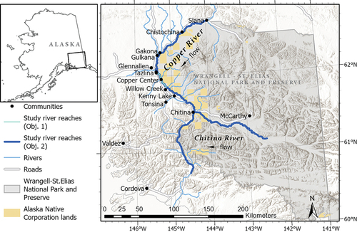
Figure 1. Study area map within the Copper River Basin of Southcentral Alaska showing Copper River and tributaries, study reaches, nearby communities, roads, boundaries of Wrangell–St. Elias National Park and Preserve, and Alaska Native Corporation lands within those boundaries. Land status from Bureau of Land Management and Alaska Department of Natural Resources and topography from Esri, FAO, NOAA, USGS.

The first objective (Objective 1) of our study was to assess the long-term changes in local river ice phenology (i.e., seasonality) and the implications for winter access. To accomplish Objective 1, we estimated river ice extent of a 30-km stretch of the Copper River on a weekly basis using the full archive of Landsat multispectral imagery (MSS/TM/ETM+/OLI sensors) from water years (WYs; begins 1 October) 1973 to 2021. We analyzed change between two roughly equal time periods and change over the time series. To infer longer-term trends beyond the remote sensing record, we established empirical relationships between local air temperature metrics and ice extent from the 1940s to the present. We expected the timing and extent of ice cover development to vary spatially along rivers, with consequences for river ice travel. Our second objective (Objective 2) was therefore to characterize the geospatial patterns of river ice navigability in recent years (WYs 2018–2021) over large portions of the Copper and Chitina rivers (~500 km). We addressed Objective 2 using two distinct approaches, with different satellite platforms, spatial scales, and temporal resolutions. First, we mapped the variation in late-winter open water area using Sentinel-2 multispectral imagery to differentiate reaches with consistent ice covers versus persistent open water and compared these patterns with hydrologic and geomorphic characteristics (e.g., channel slope, width, braiding, discharge, unit stream power) to understand potential drivers. Second, we used Sentinel-1 synthetic aperture radar (SAR) imagery to map the seasonal development of the ice cover and persistent open water. We used publicly submitted photo observations, in situ cameras, and optical satellite imagery as reference data sets for the remote sensing analyses. By investigating historical trends and the recent spatiotemporal patterns of the river ice cover, we aimed to assess the societal impacts of climate change and foster safer and more predictable access to wild resources and the landscape.

Study area

The Copper River Basin is located in the Southcentral region of Alaska. The upper basin has a continental climate with large fluctuations in temperature and low precipitation (Bieniek et al. 2012) and is underlain by discontinuous permafrost (Pastick et al. 2015). Wintertime (December–February) mean air temperature and total precipitation normals (1991–2020) for the Gulkana weather station were −17.4°C and 55 mm, respectively (Alaska Climate Research Center 2022). Below the Chugach Mountains, the maritime influence moderates air temperatures and increases precipitation (Bieniek et al. 2012), and permafrost is sporadic (Pastick et al. 2015).

This study focuses primarily on the glacially fed Copper River (~500 km), which drains a heterogeneous landscape of approximately 64,000 km² and supports prolific salmon (Oncorhynchus) runs (Figure 1). By streamflow runoff, the Copper River Basin is the second largest in the state (Ackerman et al. 2013), with glacial ice melt contributing approximately a quarter of the flow (van Beusekom and Viger 2018). The Copper River begins at the terminus of a glacier in the northern Wrangell Mountains, flows through the intermontane area, cuts through the Chugach Mountains in deep canyons, and flows into the Gulf of Alaska. The Chitina River (~200 km), which also begins at the terminus of a glacier, meets the Copper River just before the Chugach Mountains.

The Copper River Basin lies within the traditional territory of the Ahtna (Atnahwt’aene), a Northern Dene Athabaskan group (Simeone et al. 2019). The Ahtna historically lived off of the land in a semi-nomadic lifestyle, following the food sources seasonally, and traveled in winter to hunt moose (Alces alces) and caribou (Rangifer tarandus), trap furbearers, fish on frozen lakes and rivers, and gather firewood (Miller 2023). By the 1940s, life had changed significantly, with Ahtna families settling in permanent villages along the road system, mostly located by the mouths of major tributaries to the Copper River (called Atna in the Ahtna language; Simeone et al. 2019). The connection to the land and to traditional harvest practices remains central to Ahtna culture. The use of wild resources is also an important part of the lifestyle of many non-Native residents of this region. The practice of trapping, as an exclusively wintertime activity, is particularly dependent on snow and ice conditions, and winter hunting, ice fishing, and firewood collection continue to rely on safe and predictable travel across river ice.

The basin is a rural, highway-accessible region, with roads and communities now located primarily to the west of the upper Copper River (Figure 1). Historically, the Ahtna inhabited both banks of the Copper River. With only one bridge crossing the upper river, wintertime access to the land east of the river is primarily by crossing river ice. The land to the east of the river is held by several entities, primarily the U.S. federal government (Wrangell–St. Elias National Park and Preserve), Alaska Native corporations (Ahtna, Inc. and Chitina Native Corp.), and individual Native Allotments (Figure 1). Land was transferred to the Alaska Native regional and village corporations though the Alaska Native Claims Settlement Act of 1971. Ahtna, Inc. and Chitina Native Corp. own over 2,400 km² of land within the external boundaries of Wrangell–St. Elias National Park and Preserve directly east of the Copper River (Ahtna, Inc. 2022; Figure 1). At over 53,000 km², Wrangell–St. Elias is the largest national park unit in the United States. Ensuring continued access to and use of subsistence resources is among the most significant federal management priorities here. The Alaska National Interest Lands Conservation Act, the park unit’s enabling legislation, holds subsistence access and opportunity (“to provide the opportunity for rural residents engaged in a subsistence way of life to continue to do so”) on equal footing with the Act’s other purposes (ANILCA 1980). Subsistence access and opportunity are fundamental to the purpose of this park and preserve and other federal conservation units with a subsistence purpose established by the Alaska National Interest Lands Conservation Act. The climate change impacts on winter subsistence access therefore have important implications for the federal management of these lands.

Methods

Historic changes in river ice cover (Objective 1)

We used the historic archive of multispectral Landsat imagery from the National Aeronautics and Space Administration (NASA)/U.S. Geological Survey (USGS) for a retrospective analysis of river ice phenology for WYs 1973 to 2021. Data were acquired from Landsat 1 to 8 satellites, which were launched sequentially throughout this time period. The satellites were equipped with Multispectral Scanner (MSS), Thematic Mapper (TM), Enhanced Thematic Mapper Plus (ETM+), or Operational Land Imager (OLI) sensors, with spatial resolutions ranging from 30 to 60 m for the bands used in this study. The repeat orbit cycle for each Landsat satellite is sixteen days, but coverage at shorter intervals is available within the swath overlap between passes. In some time periods, the potential temporal resolution was improved with multiple satellites concurrently operational. However, there are also major gaps in imagery due to the historic privatization of the Landsat program, the low sun elevations in winter, and cloud cover.

We designed our study to maximize the number of usable Landsat images and to make inferences of ice extent between observations. We defined the region of interest within the swath overlap of satellite passes and focused on a short 30-km stretch of the Copper River to improve the potential temporal resolution of the data (Figure 1). We considered all Landsat Collection 2 Level-1 data from November to May, including Tier 1 and Tier 2 collections with all levels of cloud cover, and manually assessed each image for quality. We estimated ice extent visually, an approach that allowed us to create a more comprehensive local data set than would be possible with image classification methods that are more sensitive to image quality (e.g., shadows, haze) than the human eye.

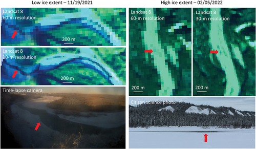
We first compared Landsat satellite imagery with concurrent ground-based photos from fixed cameras (Bondurant et al. 2022) and with citizen science observations submitted through the Fresh Eyes on Ice website or through the GLOBE Observer app (Fresh Eyes on Ice 2022; GLOBE 2022). The protocol for collecting citizen science photo observations was reviewed by the University of Alaska Fairbanks Institutional Review Board and was determined an exempt activity under 45 CFR 46 (IRB Review reference number 1,841,855–1). All photo observations were submitted to the Fresh Eyes on Ice project with free, prior, and informed consent, and contributors were informed of their use in this article. Photos from April 2021 to May 2022 were used to understand what ice conditions can be inferred from visual interpretation of the satellite imagery (Figure 2). Notes associated with citizen science photos also helped clarify the local river use under different ice conditions. In the Landsat imagery, large open leads, large areas of overflow and snowmelt, ice jams, and backwater flooding were visible at 30-m and 60-m resolutions; however, many of the poor ice conditions (open leads, overflow) occurring at subpixel scales were not visible (Figure 2). Poor ice conditions even at the 1-m scale can affect safety and navigability. This limitation affects interpretation of results, because areas that appear to be fully ice covered in the satellite imagery may have undetectable open water features that remain significant barriers or hazards for river users. Another caveat is that this study assesses only the occurrence of surface water, acknowledging that there are many other ice conditions that can negatively impact navigability and safety (e.g., overflow beneath snow, thin ice, shelf ice, rough ice).

Figure 2. Example of low (left panel) and high (right panel) ice extent classes shown for segments of the Copper River study reach north of Copper Center. Classes were assigned by interpreting Landsat images at 60-m resolution to be consistent across sensors. Landsat 8 images are shown in the resampled 60-m resolution and original 30-m resolution and are displayed as RGB composites with SWIR, NIR, and green bands. Below are photographs taken from a fixed time-lapse camera (left; Bondurant et al. 2022) and citizen science observer (right; Fresh Eyes on Ice 2022) on the same dates as the satellite image acquisitions. Open water is present in both low and high ice extents. Red arrows indicate the location of open water pictured in the photographs on the Landsat images.

We resampled the imagery from TM, ETM+, and OLI sensors to a 60-m pixel size to match the spatial resolution of the older MSS sensors. Images were interpreted as false color composites with shortwave infrared (SWIR, 0.8–1.75 μm; wavelength range across sensors), near-infrared (NIR, 0.7–0.9 μm), and green bands (0.5–0.6 μm). For each image date, we assigned categorical classes of river ice extent in the study reach by estimating the relative length of the reach that was affected by water. This metric was chosen for several reasons: (1) to address the concern of river users and land managers of the ability to cross the river (an open lead spanning the length of the reach would inhibit crossing, regardless of its width) and (2) for the ability to make rapid accurate assessments. We defined ice extent (low, moderate, high) and the implications for river ice travel (minimal, moderate, widespread opportunities for ice travel and river crossing) according to Table 1 (examples in Figure 2).

Table 1. Characteristics of ice extent classes for a 30-km segment of the Copper River by Copper Center, as interpreted from Landsat imagery.

Ice extent category	Length of river segment (%) affected by water	Implications for river ice travel
Low	>75	Minimal opportunities for crossing ice
Moderate	25–75	Potential opportunities for crossing ice in some areas
High	<25	Widespread opportunities for ice travel and crossing

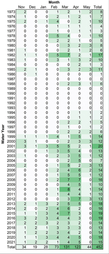
We made a total of 452 observations (unique image dates) of ice extent from the Landsat archive (Figure 3). We then gap-filled this data set between observations when possible, following a set of rules connecting the same classes within time limits specified by class and season, and summarized the data set at weekly time steps. For analysis, we ultimately simplified these into the binary classes of “high ice extent (<25 percent length with water)” and “low–moderate ice extent (>25 percent length with water).” The structure of the Landsat data set showed seasonal and historic data gaps that influence results (Figure 3). Observations surrounding the winter solstice from December to January were particularly scarce until 2013, so statistical tests were only conducted for late winter–spring (weeks 8 February–8 April). There was also a long gap from 1986 to 1995 with almost no winter observations until April. From this data set, it is difficult to quantify the absolute change in duration of the ice travel season and timing of freeze-up/breakup. Our analyses therefore focus on examining the relative proportions and probabilities of observations of high ice extent and the frequency of incomplete freeze-up.

Figure 3. Landsat data used in the analysis of historic ice phenology summarized by month and year. Cell values represent the number of unique image dates. Multiple scenes from the same image date were mosaicked together. Color scale ranges from white to green representing relatively low to high values.

We analyzed variation in ice phenology over time in several ways. First, we examined interannual variation in weekly ice extent as a matrix of gap-filled observations to identify years without the development of a complete ice cover. We then compared weekly ice extent (binary categorical response) between two roughly equal time periods (T₁ = 1973–1997, T₂ = 1998–2021; binary categorical predictor) and conducted contingency analyses with Pearson chi-square tests where there were sufficient observations (average cell count of at least five). We also analyzed trends in weekly ice extent over time (WYs 1973–2021) with simple logistic regression models for weeks with a sufficient number of observations in each class. We interpreted trends using the predicted probability of high ice extent over the time series. We then examined the strength of the relationships between weekly ice extents and local air temperature metrics with simple logistic regression. The air temperature metrics we considered included thirty-one-day prior mean air temperatures and accumulated freezing degree days (AFDD), calculated from daily mean air temperature (°C) data from National Weather Service Station USW00026425 near Gulkana (Alaska Climate Research Center 2022). Daily freezing degree days (FDD) were calculated by subtracting the daily mean air temperature from 0°C. Daily FDD is therefore positive when mean air temperature is below freezing and negative when above freezing. AFDD is the sum of daily FDD from the beginning of the WY. Weekly averages of the air temperature metrics were related to Landsat-derived weekly ice extents. Finally, we assessed the long-term trend (WYs 1943–2021) in the local air temperature metric most closely related to ice extent with simple linear regression. Statistical significance was considered strong at alpha = .05 and weak at alpha = .10.

Geospatial patterns of river ice cover and persistent open water (Objective 2)

Multispectral analysis of late-winter open water area

We expected the development of the ice cover and its impacts on accessibility and travel safety to vary spatially along rivers. To differentiate river reaches with tendencies to develop a potentially navigable ice cover versus extensive open water, we compared recent geospatial patterns of late-winter (late January/early February) open water area for the Copper and Chitina rivers (Figure 1, dark blue). We processed multispectral Sentinel-2 imagery (10-m resolution) from the European Space Agency in Google Earth Engine (Gorelick et al. 2017), identifying images with minimal cloud cover acquired at anniversary dates (within one week) over multiple recent years. Images used in this study were from: 1 February 2019, 25 January 2021 and 26 January 2021 (combined due to partial cloud cover and incomplete study area), and 31 January 2022. Images were displayed as true color and false color composites (red: SWIR, green: NIR, blue: green) to help differentiate water from dark vegetation and shadows. For each image date, we manually digitized the length and width of open water leads and summarized the area of open water by 5-km reach.

We examined flow energy as a potential control over late-winter open water area. We postulated that high flow energy may slow the development of the surface ice cover and increase late-winter open water area by limiting the thermal formation of skim ice and mechanically inhibiting the accumulation of ice floes (Prowse and Beltaos 2002; Beltaos and Prowse 2009; Shen 2010). Flow energy was represented as an estimate of unit stream power by 5-km reach, which is stream power normalized by channel width (Bagnold 1960; Gartner 2016):

$\mathit{\omega }=\frac{\mathit{\rho gQS}}{b}$

where ω is unit stream power (W/m²), $\mathit{\rho }$ is the density of water (1,000 kg/m³), $\mathit{g}$ is acceleration due to gravity (9.8 m/s²), $\mathit{Q}$ is discharge (m³/s), $\mathit{S}$ is channel slope (m/m), and $\mathit{b}$ is the channel width (m).

Discharge by reach was estimated by scaling average autumn discharge at the Copper River gaging station (ID: 15214000, Copper River at Million Dollar Bridge; USGS 2022) by the drainage area (i.e., flow accumulation), which was extracted from the digital elevation model (DEM)-derived Hydrography90 geospatial data set (Amatulli et al. 2022). Channel slope was calculated from the Copernicus GLO-30 DEM (European Space Agency). Channel width and number of channels in autumn were estimated using land masks that we created from optical, SAR, and DEM sources (see next subsection). The number of channels indicates the degree of braiding/anastomosis, which is also expected to impact the formation of the ice cover and jamming points. These hydrologic and geomorphic variables were assessed alongside open water areas for each year to understand the spatial patterns of open water persistence. We considered correlation and regression analyses to identify potential drivers of open water extent; however, the high degree of spatial autocorrelation of open water area among river reaches inflated the statistical significance of the results and challenged interpretation. We limited this analysis to the Copper River, for which discharge and unit stream power could be estimated.

SAR analysis of seasonal ice development and open water occurrence

We examined the seasonal progression of the ice cover formation and open water persistence over multiple years using Sentinel-1 C-band (5.405 GHz) SAR data (European Space Agency). This platform is advantageous for winter observation at high latitudes because it is not affected by the low-light conditions or cloud cover, which are limiting for optical remote sensing, and can have relatively high spatial and temporal resolutions, with repeat passes every twelve days. Two Sentinel-1 satellites (Sentinel-1A, Sentinel-1B) have been in orbit at different times from 2014 until the present. Scenes from these satellites have different flight geometries (ascending versus descending), resulting in different look directions, which, in high-relief settings such as this study area, result in different areas being impacted by terrain effects (shadowing and layover distortions). Using both ascending and descending passes, we found that we can achieve a more complete view of the river area by reducing the number of invalid pixels. The temporal scope of this analysis was therefore defined by the period when both satellites were operational for the freeze-up season: WYs 2018, 2019, and 2020.

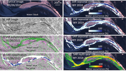
We used high-resolution Level-1 Ground Range Detected products acquired in Interferometric Wide swath mode. These products have 20 × 22 m spatial resolution, 10-m pixel size, and incidence angles ranging from 29.1° to 46.0°. Images were preprocessed in Google Earth Engine (Gorelick et al. 2017), as implemented by the Sentinel-1 Toolbox (European Space Agency, https://sentinel.esa.int/web/sentinel/toolboxes/sentinel-1), for thermal noise removal, radiometric calibration, and geometric terrain correction (using ASTER DEM; Figure 4(b)). For visualization purposes, we used this level of processing to then create multitemporal composites of VV backscatter that combined an autumn scene with each winter scene (Figure 4(c)). The autumn scene captures the extent of open water prior to the onset of freeze-up. Water typically has very low VV backscatter (though turbulence and wind can increase VV backscatter), and land and ice typically have relatively high VV backscatter (though smooth ice or ice overlain with water may have low backscatter). By compositing SAR VV backscatter intensity from autumn before freeze-up and during the winter using an RGB composite (red: autumn backscatter, green: winter backscatter, blue: autumn backscatter; Figure 4(c)), it is easier to visually differentiate ice from water and land than with a winter scene alone (Figure 4(b)). This visualization should ideally show water as black (assuming low backscatter from open water in autumn, low backscatter from open water in winter) and ice as green (assuming low backscatter from open water in autumn, high backscatter from ice in winter; Figure 4(c)). These multitemporal composites were used to help us visualize the development of the ice cover in addition to using pixel-based image classifications of water and ice.

Figure 4. Examples of Sentinel-1 SAR image processing: (a) Sentinel-2 optical reference image (true color); (b) SAR single-date image (VV backscatter); (c) SAR multitemporal composite (red: VV backscatter from autumn, green: VV backscatter from 26 January 2021, blue: VV backscatter from autumn); (d) SAR classification of water and ice for single-date using a threshold on VV, overlain on SAR multitemporal composite; (e)–(g) SAR seasonal composites of classified images showing water occurrence from November to February for WYs 2018, 2019, and 2020, overlain on optical image (Sentinel-2, 26 January 2021); and (h) SAR multiyear composite showing water occurrence from November to February averaged for WYs 2018 to 2020, overlain on optical image (Sentinel-2, 26 January 2021).

For the purpose of water/ice image classifications, we further processed the imagery. We chose gamma-naught calibration to mitigate the confounding effect that different incidence angles can introduce. We applied a radiometric slope correction with the GLO-30 DEM using a volumetric model and masked the geometric layover and shadows (Vollrath, Mullissa, and Reiche 2020). The Refined Lee Speckle filter was then used to mitigate false high and low backscatter from random phase interference (speckle), a necessary processing step that smooths the data but reduces the effective spatial resolution.

Annual pre-freeze-up land masks were created to remove non-water pixels from the classification by combining masks derived from optical imagery (Sentinel-2), SAR imagery (Sentinel-1), and a DEM (GLO-30). The optical land masks were created by applying a threshold (0.15) to the median Normalized Difference Water Index of cloud-masked imagery for autumn (September and October). This Normalized Difference Water Index threshold was selected after visually inspecting the performance over a range of thresholds to delineate water and land. Lower thresholds than this tended to misclassify wet silt bars as water. The SAR land masks were created by applying the Otsu adaptive thresholding method to an autumn image using the VV polarization. The DEM was used to exclude steep slopes >20°, because these slopes should only occur on land, not water. Finally, to exclude any pixels that were not a part of the Copper or Chitina rivers, we created river polygons using surface water extents from the Joint Research Center Global Surface Water (Pekel et al. 2016) and Alaska Hydrography (Alaska Center for Conservation Science 2019) data sets.

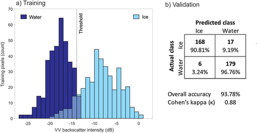
The masked Sentinel-1 SAR images from November to February for three years (WYs 2018–2020) were then classified into water and ice pixels using a threshold of VV backscatter intensity (Figure 4(d)) that was chosen through histogram analysis of a training data set (Figure 5(a)). A ground reference data set was constructed using Sentinel-2 imagery to identify 546 point locations that were water in fall 2020 and ice in winter of that season. The 1,092 ground reference points were then randomly subdivided into training and validation data sets using a 70 percent/30 percent split. We selected a VV backscatter threshold of −14 dB using the intersection of the water and ice distributions from the training data set (Figure 5(a)). The validation data set was used for quantitative accuracy assessment, and performance was further assessed visually by comparing classifications with satellite optical imagery and ground-based photos (Bondurant et al. 2022). We considered alternate classification techniques, some that have been successful in other studies of ice, including unsupervised k-means clustering (e.g., Sobiech and Dierking 2013) and Otsu thresholding (e.g., Murfitt and Duguay 2020), and supervised machine learning using support vector machines. The supervised methods (histogram slicing and support vector machines) yielded the most consistent and accurate results.

Figure 5. Sentinel-1 SAR classification of water and ice. A threshold of VV backscatter intensity (dB) was determined through histogram analysis of training pixels (a), and an accuracy assessment was conducted with a validation data set (b). Confusion matrix (b) shows predicted versus actual classes, with count of validation pixels in bold.

The individual SAR classifications were then composited for each freeze-up season (November to February) to produce maps of pixel-based water occurrence showing the percentage of scenes that a pixel was classified as water (Figure 4(e)–(g)). From these, we can visualize and infer the spatiotemporal patterns of the development of the ice cover and the persistence of open water. The seasonal composites were then averaged over multiple years to identify areas with recurring open water through winter (Figure 4(h)). The Sentinel-1 SAR scenes used to create these products are summarized in Table 2.

Table 2. Summary of Sentinel-1 SAR scenes used for analysis of river freeze-up and open water persistence for each WY by satellite.

				Count of scenes (November–February)
Satellite	Pass	Relative orbit no.	Slice no.	WY 2020	WY 2019	WY 2018
Sentinel-1A	Descending	14	4	10	10	10
		14	5	10	10	10
		14	6	10	10	10
		160	6	10	9	8
Sentinel-1B	Ascending	94	1	10	10	9
		94	2	10	10	9
		123	2	10	9	8

Data and code availability

Data and source code are available online (Brown et al. 2023).

Results and discussion

Long-term change and variability in river ice cover and accessibility (Objective 1)

This analysis provides historical documentation of changes in river ice cover and navigability evident in the record of Landsat imagery and air temperature data that complement the firsthand knowledge of local residents (Miller 2023). Our retrospective analysis was focused on a portion of the Copper River near the community of Copper Center using satellite imagery for an approximately fifty-year period from WYs 1973 to 2021. We examined variation in weekly ice extents, which were defined to represent the potential for widespread river ice travel (high ice extent) versus relative inaccessibility (low-moderate ice extent; Figure 2), acknowledging that we could not reliably detect all subpixel (<60-m) open water or other ice-related hazards that limit ice travel and safety.

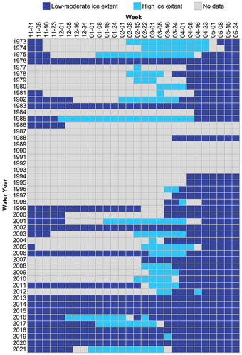
On an interannual basis, we observed substantial variation in the timing, duration, and presence of high ice extents that would enable widespread river travel (Figure 6). Winters with incomplete freeze-up, or with only one week of high ice extent, were very common in recent years: WYs 2013, 2014, 2015, 2018, 2019, 2020 (Figure 6). Though less common, winters with incomplete freeze-up were also documented in the early years of the Landsat record, including WYs 1976 and 1983 (Figure 6). There were numerous years for which we could not determine the occurrence of incomplete freeze-up due to data gaps.

Figure 6. Matrix of gap-filled ice extent observations derived from Landsat imagery for the 30-km study reach of the Copper River near Copper Center, summarized by week and water year.

Comparing weekly ice extent between the approximately equal time periods of WYs 1973–1997 with WYs 1998–2021, we found that the more recent time period had a consistently lower proportion of observations of high ice extents for the full freeze-up through breakup cycle (Figure 7); however, the sample sizes for the former period were much smaller, increasing the uncertainty of the results (Figure 6). The statistical significance of these differences in ice extent among time periods were strongest in late winter (second and third weeks of February; p = .02–0.03) and ranged from nonsignificant to weakly significant (p = .06–0.23) for the other six weeks tested (Figure 7). For the WYs 1973–1997 time period, there was an eight-week period (first week of February through last week of March) where the majority of weekly observations (>50 percent) were of high ice extents (Figure 7). By contrast, the WYs 1998–2021 time period only had a two-week period (first and second weeks of March) where the majority of observations were of high ice extents (Figure 7).

Figure 7. Weekly occurrence of high ice extent expressed as percentage of total Landsat-derived observations by time period (WYs 1973–1997 and WYs 1998–2021) for the Copper River study reach, showing the reduced occurrence of high ice extents in the recent time period. The majority of weekly observations by time period were of high ice extents for the points above the dashed reference line (>50 percent). Statistical significance of weekly contingency analyses conducted from 8 February through 8 April is denoted as *p < .1 and **p < .05.

Logistic regression analyses of change over time (WYs 1973–2021) in weekly ice extent showed significant declines in the probability of high ice extents throughout the late winter (8 February) through spring (8 April; p = .007–0.09; Figure 8(a), Table 3), suggesting trends toward delayed freeze-up and earlier breakup. Though the statistical significance of these trends was greater in the breakup season, the relative difference in the strength of the trends between seasons is difficult to interpret due to the smaller sample size within the freeze-up season. The magnitude of change was large in both times of year. Between WYs 1973 and 2021, the probability of weekly high ice extent occurrence declined by an average of 53.3 (±6.6) percentage points (difference in percentages, not the percentage change; Figure 8(b)). For example, the probability of high ice extent between WYs 1973 and 2021 declined from 74 to 17 percent for the second week of February, from 89 to 37 percent for the second week of March, and from 48 to 1 percent for the second week of April (Figure 8(b)). For WY 1973, ice extent was most likely high (ranging from 68 to 89 percent probability) for eight of the nine weeks tested (8 February–1 April), whereas for WY 2021, high ice extent was unlikely (ranging from 7 to 40 percent probability) for this same time span.

Figure 8. Change over time in the probability of high ice extents on Copper River study reach from logistic regression analyses of Landsat-derived observations. (a) Weekly probability curves over the full time series (WYs 1973–2021) and (b) comparison of probability between the first and last years of the time series (WYs 1973 and 2021). Decreasing trends in probability of high ice extents were found for all weeks tested. Statistical significance was denoted as *p < .1, **p < .05, ***p < .01.

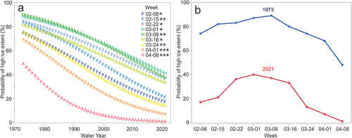
Table 3. Logistic regression models for log odds of high ice extent (derived from Landsat imagery) for Copper River (30-km study reach by Copper Center) by WY (1973–2021) for each week from late winter (8 February) to spring (8 April).

Week	n	Chi-square	p Value	Intercept	Parameter estimate
8 February	20	3.7	.05	109.2	−0.06
15 February	25	5.4	.02	119.4	−0.06
22 February	26	3.1	.08	90.5	−0.05
1 March	29	3.3	.07	96.6	−0.05
8 March	29	4.2	.04	108.4	−0.05
16 March	32	2.8	.09	87.9	−0.04
24 March	35	5.9	.02	120.8	−0.06
1 April	36	7.0	.008	139.4	−0.07
8 April	38	7.3	.007	198.4	−0.10

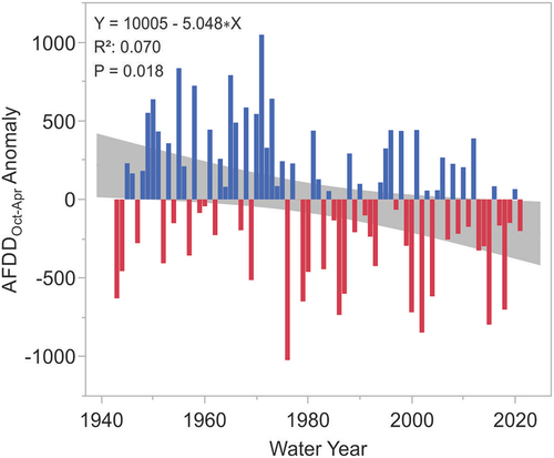
To infer longer-term changes (WYs 1943–2021) in ice extent for our study reach beyond the years of the Landsat record, we first examined relationships between our observations and metrics of local air temperature. As a cumulative measure of freezing degree days since the start of the hydrologic year (1 October), AFDD was expected to align primarily with the formation of the river ice cover, though AFDD is also balanced by thawing degree days, which was expected to impact ice decay. We found that AFDD was strongly related to weekly ice extent for most of the winter–spring period tested (8 February–1 April, p = .016–0.0003), with the strongest relationships found deeper in the winter through mid-March, when ice covers are mainly developing (Figure 9). In some years, warmer air temperatures had initiated snow/ice melt by mid-March (Figure 6). At this point in the season, thirty-one-day-prior air temperature means also became significant predictors of ice extent (16 March–1 April, p = .001–0.037; Figure 9), because springtime weather is the primary control on ice decay and breakup timing (Beltaos and Prowse 2009). AFDD_Oct-Apr for the full potential ice season were calculated to represent climatic conditions relevant to both river ice formation and decay. Despite high interannual to multidecadal variability, we found that AFDD_Oct-Apr decreased by 15% from WY 1943 to 2021 (−50 AFDD_Oct-Apr/decade; Figure 10, p = .018), suggesting a long-term change over the last approximately eighty years toward warmer conditions and reduced ice cover through the freeze-up to breakup cycle.

Figure 9. Statistical significance of relationships between weekly Copper River ice extent and climate indices (AFDD and thirty-one-day prior mean air temperature). LogWorth (−log(p value)) is shown as a measure of statistical significance for ease of visualization, with dotted reference lines indicating equivalent p values. Weekly ice extent was significantly related to AFDD throughout this time period and with thirty-one-day prior mean air temperature during March and early April.

Figure 10. Trend and variation in AFDD_Oct-Apr anomaly from WYs 1943 to 2021, derived from local daily mean air temperatures. Positive anomalies (colder than average) are shown with blue bars and negative anomalies (warmer than average) are shown in red. Statistics for simple linear regression are reported with the 95 percent confidence interval for the mean response shown in gray, indicating a 15% decline in AFDD_Oct-Apr and a long-term warming trend.

Our analyses suggest that the formation of an ice cover conducive to travel (high ice extent) has shifted to later in the winter, that incomplete freeze-ups (low–moderate ice extent throughout winter) have become more common, and that breakup initiation has advanced to earlier in the springtime. The reduced and sometimes nonexistent periods of widespread ice cover limit the ability of residents to cross the river near their communities. The changes we observed with remote sensing are consistent with a study of traditional ecological knowledge where local residents reported a decline in the ice cover beginning in the 1970s that led some to cease traveling on the ice and crossing the Copper River and contributed to decisions to abandon the practice of trapping in the following decades (Miller 2023). One respondent indicated that the river stopped freezing up reliably about twenty years ago (Miller 2023), which aligns with our satellite-based finding that there was only one week or less of high ice extent at our study reach for many years since 2000. Crossing the Copper River in the past was described as uneventful and straightforward, whereas today there is great difficulty in finding a suitable place to cross in this part of the river. One respondent from the Kenny Lake area, however, indicated that he is still able to navigate and cross the river in winter (Miller 2023). This divergent experience of changing ice conditions may be influenced by the spatial variability in patterns of ice cover development along the river, discussed in the following subsection.

A decrease in the duration of river ice cover has been detected in studies spanning the Northern Hemisphere and the globe (Magnuson et al. 2000; Bennett and Prowse 2010; Park et al. 2016; Yang, Pavelsky, and Allen 2020). Globally, Alaska has exhibited some of the largest declines in winter river ice extent (between 1984–1994 and 2008–2018), as did the Tibetan Plateau and Eastern Europe (Yang, Pavelsky, and Allen 2020). Changing ice phenology within other regions of Alaska has been reported (Herman-Mercer, Schuster, and Maracle 2011; Carothers et al. 2014; Brown et al. 2018; Cold et al. 2020), but the regional variation has not yet been well described and is the subject of future research. Though it is difficult to compare results across studies, the quantitative and qualitative changes in ice phenology and the impacts on human use described for the Copper River appear to be particularly pronounced (Miller 2023). As the climate continues to warm through the twenty-first century, the duration of ice cover is projected to decrease and the geographic zones of shorter ice durations are projected to shift further northward (Prowse et al. 2011; Yang, Pavelsky, and Allen 2020). With the ubiquity of remote sensing products throughout the Circumpolar North and the interest from stakeholders to engage in locally relevant research, our approach could be applied elsewhere to better quantify river ice trends and foster travel safety.

Geospatial patterns in river ice cover and open water occurrence (Objective 2)

To assess geospatial variation in accessibility, we calculated open water area from Sentinel-2 multispectral imagery at late-winter anniversary dates for three years (WYs 2018, 2020, and 2021) and compared these with hydrologic and geomorphic characteristics of the rivers (Figures 11 and 12). We also examined Sentinel-1 SAR imagery and derived products of water occurrence in WYs 2018 to 2020 to visualize the seasonal spatiotemporal progression of freeze-up (Figure 13).

Figure 11. Geospatial patterns of late-winter open water area (top panel) and hydrologic characteristics (bottom panel) of Copper and Chitina rivers by 5-km reach. Numbers along the Copper River indicate river-km at tributaries that demarcate reaches with distinct hydrologic characteristics referenced in Figure 12. Total areas of open water in late winter were calculated from Sentinel-2 multispectral images acquired in the WY on dates indicated. Hydrologic characteristics include river slope, flow accumulation, cumulative channel width, and unit stream power. Flow direction is indicated by arrows, and nearby communities are shown. Study reaches with no data are depicted in gray.

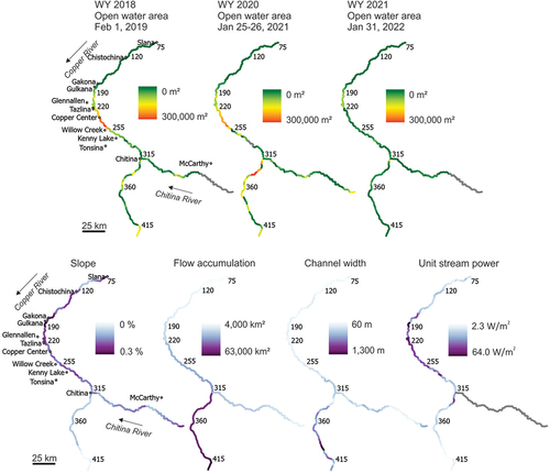
Figure 12. Profile of late-winter open water area and hydrologic characteristics of the Copper River by 5-km subreach. Solid vertical lines indicate locations of tributaries used to demarcate reaches with distinct characteristics. Names of these tributaries are shown in bold italics. Dotted vertical line shows the location of a canyon that influences hydrology. The locations of nearby communities are indicated with normal text. Open water areas were derived from Sentinel-2 imagery from late January/early February in the WYs indicated.

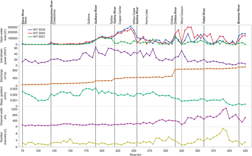
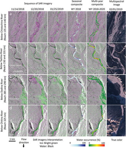
Figure 13. Examples of the freeze-up progression and open water occurrence along distinct stretches of the Copper River with Sentinel-1 SAR imagery and Sentinel-2 multispectral imagery (European Space Agency). The sequence of SAR imagery from three winter dates in WY 2018 are composites that include an autumn scene (open water prior to freeze-up) and a winter scene (red: VV autumn, green: VV winter, blue: VV autumn) and were used to optimize visualization of open water (black) and ice cover (bright green). The seasonal composite is a classified SAR product showing pixel-based water occurrence as a percentage of scenes for the season November to February in WY 2018, overlain on a SAR image. The multiyear composite shows the average water occurrence for November to February over three years (WYs 2018, 2019, 2020) to identify places that tend to remain open late in the winter year after year. The multispectral image (Sentinel-2) was used to calculate late-winter open water area and validate SAR imagery and products.

Validation of the SAR classification suggested high overall accuracy (93.78 percent, Cohen’s kappa statistic = 0.88; Figure 5), though we noticed that the performance varied along the length of the Copper River. The optimal threshold between classes likely differs across river reaches and ice covers with different physical characteristics that influence microwave scattering. Wind, turbulence, roughness at the ice–water interface, water above ice (overflow, melt ponds), floating versus bedfast ice, and sediment load all impact backscatter and can complicate the classifications. Inclusion of non-river pixels was an apparent source of error along steep terrain and within braided channels. Undetected river pixels from the land mask also resulted in gaps of valid data in the classifications. Despite these challenges, interpretation of the derived SAR products yielded insights to the patterns and processes of ice cover development in this area.

The extent of late-winter open water varied among years; however, some clear geospatial patterns emerged that can help guide decisions related to local river ice travel and access (Figures 11–13). Much of this geographic variation in persistent open water we attribute to patterns of stream flow energy and river morphology affecting the development of the ice cover. Below, we discuss our findings of the local development of the ice cover from upstream to downstream reaches of the Copper River.

From the multispectral image analysis, we found that a segment of the upper Copper River between the communities (and tributaries) of Slana to Gakona had consistently low areas of open water in late winter (Figures 11 and 12). This area was characterized by low discharge and, consequently, low unit stream power, and had narrow channels and some braided reaches (Figures 11–13). The low energy and morphology of this reach are both conducive to formation of the ice cover. Freeze-up typically begins with the development of border ice along banks, which expands laterally over time either through the thermal growth of skim ice or the accumulation of surface ice floes, both of which are limited by flow velocity (Shen 2010). The development of a complete ice cover is also enhanced by the physical structure of narrower, sinuous reaches, because the border ice has a shorter distance to span and river bends provide jamming points that fill with flowing ice and accelerate the upstream advancement of the ice front (Shen 2010; Chu and Lindenschmidt 2019).

Open water areas tended to increase immediately downstream as large tributaries like the Gulkana and Tazlina rivers increased river discharge and unit stream power to the highest levels observed throughout the Copper River (Figures 11 and 12). We expected the greater volume of fast-moving and mixing water to physically and thermally inhibit the formation of an ice cover (Prowse and Beltaos 2002; Beltaos and Prowse 2009; Shen 2010). This stretch of river was notable for expansive open water areas and large contiguous leads preventing crossings in the WYs 2018 and 2020, from the Sentinel-2 multispectral image analysis (Figures 11 and 12). The Sentinel-1 SAR imagery and seasonal composites for WYs 2018, 2019, and 2020 also showed extensive open water occurrence here (Figure 13(b)). The SAR multiyear composite highlighted the tendency for delayed and incomplete freeze-up in this stretch, with abundant open water throughout winter (Figure 13(b)). The gradual expansion of border ice and narrowing of open leads were apparent through the SAR imagery sequence (Figure 13b). Although this sequence suggests full bridging of the ice cover late in the season at river bends in WY 2018, the multispectral imagery shows that a contiguous lead remained open at least through the end of January (Figure 13(b)). We believe the high flow energy and morphology of this predominantly single-channeled meandering stretch limited the development of a contiguous ice cover. Note that our retrospective analysis of changing ice conditions using Landsat imagery and pre-satellite meteorological data near Copper Center (see previous subsection) was located within this area currently characterized by large open leads.

In WY 2021, freeze-up occurred more rapidly and late-winter open water areas were lower along most of the Copper River but remained high between the Gulkana and Tazlina rivers (Figures 11 and 12). The spatial progression of freeze-up on these high-energy reaches appeared to be influenced by the upstream advancement of the ice front from lower reaches. Below the confluence with the Dadina River, we saw a distinct decline in open water area relative to upstream reaches in WYs 2018 and 2020, despite the high discharge and unit stream power at this location (Figure 12). We attribute this to the difference in the downstream river morphology and its upstream effects on ice accumulation: the river becomes more braided (number of channels), the cumulative width increases, and slope gradient decreases from the Dadina River to Chitina River, which both lowers the stream flow energy and provides a physical structure more conducive to the development of a contiguous ice cover (Figure 12). The SAR imagery showed lateral ice growth causing narrow open leads and constrictions that filled with ice and progressed upstream relatively early in the season (Figure 13(c)). Narrow open leads in this reach sometimes persisted while ice continued to advance above them. We also saw evidence of new leads opening throughout winter.

Copper River discharge rises in-step below the confluence with the Chitina River, contributing in some years to high areas of open water (Figures 11 and 12). Interestingly, a narrow canyon in this reach that was characterized by a spike in unit stream power had consistently low areas of late-winter open water (Figure 12). SAR imagery confirmed that this canyon typically acquired an early ice cover, leading to ice accumulation upstream while open water remained downstream (Figure 13(d)). Despite high flow energy at the canyon, the narrow morphology likely promotes bridging of the border ice with the accumulation of ice pans.

The interactions among flow energy, morphology, and the upstream and downstream effects in the development of the ice cover create local variation in ice conditions that impacts navigability and access to the landscape. Here, when describing access, we refer only to open water extent that we detected with 10- to 20-m resolution satellite imagery, though other ice conditions may inhibit travel and present risks. Beyond the development of a contiguous ice cover, the ice needs to be of sufficient thickness to support travel. In future research, consideration of thin ice and other dangerous conditions such as overflow and smaller open leads would help to further refine our assessment of ice navigability. Based on open water extent alone, however, we found that the stretch of the Copper River between Tazlina and Willow Creek was notable for its persistent large open leads that have prevented crossing through late winter in some recent years. However, the stretch of river from Slana to Gakona consistently had little detectable open water by late winter and may therefore provide the most reliable opportunities for community-accessible ice travel and crossings (Figures 11 and 12). The area between Willow Creek and Chitina may also provide earlier opportunities for crossing relative to the reaches directly upstream.

Conclusions

Our study suggests a striking decline in the duration of the season for river ice travel on a stretch of the Copper River due to increasing air temperatures, from a delayed or incomplete freeze-up through an early onset of breakup. This finding echoes the experiences and concerns of local residents who can no longer predictably and safely access hunting and gathering areas, private land, and public land located across the river from their communities (Miller 2023). With projected increases in air temperature, precipitation, and river discharge in the Copper River Basin over the next century (Valentin, Hogue, and Hay 2018), we can expect the duration and the contiguity of the river ice cover to continue to decline and the activities that depend on the ice cover to be further challenged.

Our study also showed geospatial variation in freeze-up and open water occurrence along the river, patterns that appear to be driven by flow energy, channel form, and the bidirectional effects of ice flow and accumulation. The patterns we observed here are congruent with known processes of ice cover formation. The local morphology and hydrology of this river create a mosaic of ice cover conditions that affect access throughout the winter. In other regions where climatic conditions have become marginal for sustaining a reliable ice cover, rivers may also exhibit such spatial heterogeneity in the ice cover that impacts human use. By mapping the local variation in the ice cover, we identified potential winter river crossing areas and areas prone to open water persistence, which may help improve travel safety and preparedness. The remote sensing approaches we developed to monitor and map freeze-up and open water occurrence can be applied elsewhere to support local decision making and adaptation in response to rapidly changing environmental conditions in other high-latitude regions.

Acknowledgments

We thank Allen Bondurant, Caroline Ketron, and Paul Atkinson for maintaining cameras; all of the citizen science ice observers; the Fresh Eyes on Ice team; and the NASA GLOBE Observer program.

Disclosure statement

No potential conflict of interest was reported by the authors.

Additional information

Funding

This project was supported by the U.S. Department of Interior, National Park Service [P20AC00031]; the National Science Foundation Arctic Observing Network and Navigating the New Arctic programs [1836523]; NASA Citizen Science for Earth Systems Program [80NSSC21K0858 and 80NSSC22K1915]; the Interdisciplinary Research for Arctic Coastal Environments (InteRFACE) project through the U.S. Department of Energy, Office of Science, Biological and Environmental Research; and the Bonanza Creek LTER, which is funded jointly by the National Science Foundation [DEB-1636476] and the USDA Forest Service, Pacific Northwest Research Station [RJVA-PNW-01-JV-11261952-231].

References

- Ackerman, M. W., W. D. Templin, J. E. Seeb, and L. W. Seeb. 2013. Landscape heterogeneity and local adaptation define the spatial genetic structure of Pacific salmon in a pristine environment. Conservation Genetics 14, no. 2: 483–18. doi:10.1007/s10592-012-0401-7.
- Ahtna Inc. 2022. Website. www.ahtna.com (accessed January 1, 2022).
- Alaska Center for Conservation Science. 2019. Alaska hydrography database. Alaska Center for Conservation Science, University of Alaska Anchorage. http://akhydro.uaa.alaska.edu/data/ak-hydro/ (accessed December 14, 2019)
- Alaska Climate Research Center. 2022. Data portal. https://akclimate.org/data/data-portal/.
- Alaska National Interest Lands Conservation Act (ANILCA). 1980. Public Law 96-487. 94 Stat 2371.
- Amatulli, G., J. Garcia Marquez, T. Sethi, J. Kiesel, A. Grigoropoulou, M. Üblacker, L. Shen, and S. Domisch. 2022. Hydrography90m: A new high-resolution global hydrographic dataset. Earth System Science Data Discussion 2022, no. February: 1–43.
- Bagnold, R. A. 1960. Sediment discharge and stream power–A preliminary announcement: US Geological Survey, circular 421.
- Beltaos, S., and T. Prowse. 2009. River-ice hydrology in a shrinking cryosphere. Hydrological Processes 23, no. 1: 122–44. doi:10.1002/hyp.7165.
- Bennett, K. E., and T. D. Prowse. 2010. Northern Hemisphere geography of ice-covered rivers. Hydrological Processes 24: 235–40.
- Bieniek, P. A., U. S. Bhatt, L. A. Rundquist, S. D. Lindsey, X. Zhang, and R. L. Thoman. 2011. Large-scale climate controls of interior Alaska river ice breakup. Journal of Climate 24, no. 1: 286–97. doi:10.1175/2010JCLI3809.1.
- Bieniek, P. A., U. S. Bhatt, R. L. Thoman, H. Angeloff, J. Partain, J. Papineau, F. Fritsch, et al. 2012. Climate divisions for Alaska based on objective methods. Journal of Applied Meteorology and Climatology 51, no. 7: 1276–89. doi:10.1175/JAMC-D-11-0168.1.
- Bondurant, A., C. Arp, D. Brown, and K. Spellman. 2022. Alaska river ice phenology camera network - 2019-2022. Arctic Data Center.
- Brinkman, T., B. Charles, B. Stevens, B. Wright, S. John, B. Ervin, J. Joe, et al. 2022. Changes in sharing and participation are important predictors of the health of traditional harvest practices in Indigenous communities in Alaska. Human Ecology 50, no. 4: 681–95. doi:10.1007/s10745-022-00342-4.
- Brown, D., C. Arp, T. Brinkman, B. Cellarius, M. Engram, M. Miller, and K. Spellman. 2023. River ice and open water extent from satellite imagery, Copper River Basin, Alaska (1973–2022). Arctic Data Center. doi:10.18739/A21V5BF8T.
- Brown, D. R. N., T. J. Brinkman, G. P. Neufeld, L. S. Navarro, C. L. Brown, H. S. Cold, B. L. Woods, and B. L. Ervin. 2022. Geospatial patterns and models of subsistence land use in rural Interior Alaska. Ecology and Society 27, no. 2. doi:10.5751/ES-13256-270223.
- Brown, D. R. N., T. J. Brinkman, D. L. Verbyla, C. L. Brown, H. S. Cold, and T. N. Hollingsworth. 2018. Changing river ice seasonality and impacts on interior Alaskan communities. Weather, Climate, and Society 10, no. 4: 625–40. doi:10.1175/WCAS-D-17-0101.1.
- Carothers, C., C. Brown, K. J. Moerlein, J. Andrés López, D. B. Andersen, and B. Retherford. 2014. Measuring perceptions of climate change in Northern Alaska: Pairing ethnography with cultural consensus analysis. Ecology and Society 19, no. 4. doi:10.5751/ES-06913-190427.
- Chu, T., and K. E. Lindenschmidt. 2019. Effects of river geomorphology on river ice freeze-up and break-up rates using MODIS imagery. Canadian Journal of Remote Sensing 45, no. 2: 176–91. doi:10.1080/07038992.2019.1635004.
- Cold, H. S., T. J. Brinkman, C. L. Brown, T. N. Hollingsworth, D. R. N. Brown, and K. M. Heeringa. 2020. Assessing vulnerability of subsistence travel to effects of environmental change in interior Alaska. Ecology and Society 25, no. 1. doi:10.5751/ES-11426-250120.
- Fleischer, N. L., P. Melstrom, E. Yard, M. Brubaker, and T. Thomas. 2014. The epidemiology of falling-through-the-ice in Alaska, 1990-2010. Journal of Public Health (Oxford, England) 36, no. 2: 235–42. doi:10.1093/pubmed/fdt081.
- Fresh Eyes on Ice. 2022. Ice observer, fresh eyes on ice. University of Alaska Fairbanks. https://obs.feoi.axds.co/observations/
- Gartner, J. 2016. Stream power: Origins, geomorphic applications, and GIS procedures. Water Publications. 1. Retrieved from https://scholarworks.umass.edu/water_publications/1
- Gerlach, S. C., and P. A. Loring. 2013. Rebuilding northern foodsheds, sustainable food systems, community well-being, and food security. International Journal of Circumpolar Health 72, no. 1: 21560. doi:10.3402/ijch.v72i0.21560.
- GLOBE. 2022. GLOBE (Global Learning and Observations to Benefit the Environment) Program. NASA. www.observer.globe.gov
- Gorelick, N., M. Hancher, M. Dixon, S. Ilyushchenko, D. Thau, and R. Moore. 2017. Google Earth Engine: Planetary-scale geospatial analysis for everyone. Remote Sensing of Environment 202: 18–27. doi:10.1016/j.rse.2017.06.031.
- Heeringa, K. M., O. Huntington, B. Woods, I. Chapin, F. Stuart, R. E. Hum, and T. J. Brinkman. 2019. A holistic definition of healthy traditional harvest practices for rural Indigenous communities in Interior Alaska. Journal of Agriculture, Food Systems, and Community Development 9: 115–29.
- Herman-Mercer, N., P. Schuster, and K. Maracle. 2011. Indigenous observations of climate change in the Lower Yukon River Basin, Alaska. Human Organization 70, no. 3: 244–52. doi:10.17730/humo.70.3.v88841235897071m.
- Inuit Circumpolar Council–Alaska. 2015. Alaskan Inuit food security conceptual framework: How to assess the Arctic from an Inuit perspective.
- Knoll, L. B., S. Sharma, B. A. Denfeld, G. Flaim, Y. Hori, J. J. Magnuson, D. Straile, and G. A. Weyhenmeyer. 2019. Consequences of lake and river ice loss on cultural ecosystem services. Limnology and Oceanography Letters 4, no. 5: 119–31. doi:10.1002/lol2.10116.
- Loring, P. A., and S. C. Gerlach. 2009. Food, culture, and human health in Alaska: An integrative health approach to food security. Environmental Science and Policy 12, no. 4: 466–78. doi:10.1016/j.envsci.2008.10.006.
- Magnuson, J. J., D. M. Robertson, B. J. Benson, R. H. Wynne, D. M. Livingstone, T. Arai, R. A. Assel, et al. 2000. Historical trends in lake and river ice cover in the Northern Hemisphere. Science 289, no. 5485: 1743–6. doi:10.1126/science.289.5485.1743.
- Miller, O. 2023. Wintertime travel, access, and changing snow and ice conditions in Alaska’s Copper River basin. Natural Resources Report NPS/WRST/NRR-2023/2508.
- Murfitt, J., and C. R. Duguay. 2020. Assessing the performance of methods for monitoring ice phenology of the world’s largest high Arctic lake using high-density time series analysis of Sentinel-1 data. Remote Sensing 12, no. 3: 1–24. doi:10.3390/rs12030382.
- Park, H., Y. Yoshikawa, K. Oshima, Y. Kim, T. Ngo-Duc, J. S. Kimball, and D. Yang. 2016. Quantification of warming climate-induced changes in terrestrial Arctic river ice thickness and phenology. Journal of Climate 29, no. 5: 1733–54. doi:10.1175/JCLI-D-15-0569.1.
- Pastick, N. J., M. T. Jorgenson, B. K. Wylie, S. J. Nield, K. D. Johnson, and A. O. Finley. 2015. Distribution of near-surface permafrost in Alaska: Estimates of present and future conditions. Remote Sensing of Environment 168: 301–15. doi:10.1016/j.rse.2015.07.019.
- Pekel, J.-F., A. Cottam, N. Gorelick, and A. S. Belward. 2016. High-resolution mapping of global surface water and its long-term changes. Nature 540, no. 7633: 418–22. doi:10.1038/nature20584.
- Prowse, T., K. Alfredsen, S. Beltaos, B. Bonsal, C. Duguay, A. Korhola, J. McNamara, et al. 2011. Past and future changes in Arctic lake and river ice. Ambio 40, no. SUPPL. 1: 53–62. doi:10.1007/s13280-011-0216-7.
- Prowse, T. D., and S. Beltaos. 2002. Climatic control of river-ice hydrology: A review. Hydrological Processes 16, no. 4: 805–22.
- Shen, H. T. 2010. Mathematical modeling of river ice processes. Cold Regions Science and Technology 62, no. 1: 3–13.
- Simeone, W. E., W. Justin, M. Anderson, and K. Martin. 2019. The Ahtna homeland. Alaska Journal of Anthropology 17, no. 1&2: 102–19.
- Sobiech, J., and W. Dierking. 2013. Observing lake- and river-ice decay with SAR: Advantages and limitations of the unsupervised k-means classification approach. Annals of Glaciology 54, no. 62: 65–72. doi:10.3189/2013AoG62A037.
- U.S. Geological Survey. 2022. National water information system: Web Interface. https://waterdata.usgs.gov/
- Valentin, M. M., T. S. Hogue, and L. E. Hay. 2018. Hydrologic regime changes in a high-latitude glacierized watershed under future climate conditions. Water (Switzerland) 10, no. 2: 128. doi:10.3390/w10020128.
- van Beusekom, A. E., and R. J. Viger. 2018. A physically based daily simulation of the glacier-dominated hydrology of the Copper River Basin, Alaska. Water Resources Research 54, no. 7: 4983–5000. doi:10.1029/2018WR022625.
- Vollrath, A., A. Mullissa, and J. Reiche. 2020. Angular-based radiometric slope correction for Sentinel-1 on Google Earth engine. Remote Sensing 12, no. 11: 1–14. doi:10.3390/rs12111867.
- Wheeler, P., and T. Thornton. 2005. Subsistence research in Alaska: A thirty year retrospective. Alaska Journal of Anthropology 3, no. 1: 69–103.
- Wolfe, R. J. 2004. Local traditions and subsistence: A synopsis from twenty-five years of research by the State of Alaska, technical paper 284. Alaska Department of Fish and Game.
- Wolfe, R. J., and R. J. Walker. 1987. Subsistence economies in Alaska : Productivity, geography, and development impacts. Arctic Anthropology 24, no. 2: 56–81.
- Yang, X., T. M. Pavelsky, and G. H. Allen. 2020. The past and future of global river ice. Nature 577, no. 7788: 69–73. doi:10.1038/s41586-019-1848-1.