Drivers of winter ice formation on Arctic water bodies in the Lena Delta, Siberia

ABSTRACT

Arctic landscapes are characterized by diverse water bodies, which are covered with ice for most of the year. Ice controls surface albedo, hydrological properties, gas exchange, and ecosystem services, but freezing processes differ between water bodies. We studied the influence of geomorphology and meteorology on winter ice of water bodies in the Lena Delta, Siberia. Electrical conductivity (EC) and stable water isotopes of ice cores from four winters and six water bodies were measured at unprecedented resolution down to 2-cm increments, revealing differences in freezing systems. Open-system freezing shows near-constant isotopic and EC gradients in ice, whereas closed-system freezing shows decreasing isotopic composition with depth. Lena River ice displays three zones of isotopic composition within the ice, reflecting open-system freezing that records changing water sources over the winter. The isotope composition of ice covers in landscape units of different ages also reflects the individual water reservoir settings (i.e., Pleistocene vs. Holocene ground ice thaw). Ice growth models indicate that snow properties are a dominant determinant of ice growth over winter. Our findings provide novel insights into the winter hydrochemistry of Arctic ice covers, including the influences of meteorology and water body geomorphology on freezing rates and processes.

KEYWORDS:

• Lake ice
• river ice
• stable isotopes
• Arctic
• Lena Delta

Introduction

The Arctic is currently warming nearly four times faster than the global average (Rantanen et al. 2022). As a consequence, winter ice covers of Arctic water bodies are decreasing in both thickness and duration (Prowse et al. 2011; Surdu et al. 2014). Dark, open water surfaces absorb the sun’s heat instead of reflecting it as ice does, speeding up the warming process even further. Thus, changes to Arctic winter ice covers contribute to global warming.

Some Arctic rivers and associated deltas are among the world’s largest, including the Lena Delta. Because seasonally ice-covered water bodies dominate these continuous permafrost landscapes areally, they are expected to play a major role in current and future changes to the Arctic and global hydrological cycles. However, though the role of retreating sea ice has been highlighted in this context (e.g., Bailey et al. 2021), terrestrial water sources, their ice covers, and their specific role in the climate system have received less attention.

The decline in ice cover duration and thickness that has occurred during the past century in the Northern Hemisphere is predicted to continue (Dibike et al. 2011; Shiklomanov and Lammers 2014; Sharma et al. 2019; Li et al. 2022). The internal responses of water bodies to global warming, however, are still to be understood. Ice covers control essential internal dynamics and ecosystem functions such as heat storage, permafrost thaw, winter water supply, and aquatic winter and summer habitats. A reduced ice cover may lead to increased heat storage and larger areas of unfrozen soil in otherwise continuous permafrost areas (Arp et al. 2012). Many studies show how lake ice change is driving ecological and socioeconomic change in the Arctic. For instance, an increase in aquatic plant and algae growth can lower oxygen levels due to higher decomposition rates (Griffiths et al. 2017; Bégin et al. 2021; Budy et al. 2022), and with warmer water temperatures, fish habitats, traditional harvesting methods, and the possibility of transportation via ice roads will change, impacting local communities (Prowse et al. 2011).

Numerous studies have illustrated the importance of winter ice covers as archives of winter freezing processes (Gibson and Prowse 1999, 2002; Walter Anthony et al. 2010; Wik et al. 2011; Boereboom et al. 2012; Taulu 2022). Because the geomorphology of a water body influences its hydrological flux over the course of the year, literature often differentiates between open- and closed-system freezing as described by Gibson and Prowse (1999). In recent years, different lake types in the central Lena Delta have been investigated for both summer and winter conditions (e.g., Fedorova et al. 2015; Langer et al. 2015; Skorospekhova et al. 2018). Only very few studies, however, have compared ice formation on different water body types in the same study area (e.g., Antonova et al. 2016; Spangenberg et al. 2020).

The variability of ice chemistry over the winter and its differences across water body types are a consequence of diverse water sources such as snowmelt, precipitation intermittency, and hydrological processes such as evaporation. In contrast to areas of discontinuous permafrost, where surface water bodies are partly influenced by groundwater inflow, the continuous permafrost in the study area acts as an almost impermeable layer of frozen soil (French 2007), where groundwater influx to lakes is restricted to open talik areas. This, in combination with low topographic gradients, leads to very limited water drainage and runoff (Muster et al. 2019). Groundwater movement is restricted to taliks—areas of unfrozen sediment below water bodies or enclosed lenses of unfrozen soil within permafrost—and lateral groundwater movement is generally confined to the active layer in summer. Therefore, the main water sources for surface water bodies in the study area are snowmelt in spring and precipitation in summer, whereas in winter, water influx is usually completely prevented by frozen ground.

Hydrochemical signatures within the ice react very sensitively to climate conditions. In addition, pan-Arctic river sampling programs such as ArcticGRO (since 2009) and, more recently, the Lena River Water Monitoring Program that ran from 2018 to 2022 at the research station on Samoylov Island (Juhls et al. 2020; Holmes et al. 2021) have provided valuable insights into seasonal change in river water hydrochemistry. This allows correlation between river water and ice hydrochemistry data.

The goal of this study is to better understand the links between the characteristics of water bodies, ice formation, and local winter weather. We aim to identify how local conditions such as changing water sources, winter air temperatures, and snowfall drive ice formation on Arctic surface water bodies and how this can be simulated realistically. We look at ice covers across different types of water bodies to test whether they can provide information on their geomorphological characteristics (e.g., depth and freezing system), main water sources, hydrological connections to other water bodies, and the age of the landscape unit that they are located in. We hypothesize the following:

1. The depth of a lake is a proxy for lake and talik volume and reflects the freezing system conditions (i.e., open- or closed-system freezing) in the winter ice cover.

2. Besides water body depth, snow is the main (external) control of ice cover formation over winter.

3. Meteorological data (i.e., winter air temperatures and snow depths) may be used to predict ice growth on Arctic lakes and rivers (i.e., for floating-ice regimes) and directly link it to water body chemistry in winter.

Study area

Our study was conducted in the Lena Delta in Northeast Siberia, the largest river delta in the Arctic (Figure 1). The Lena Delta covers about 29,000 km² (Schneider, Grosse, and Wagner 2009). As the Lena River reaches the Laptev Sea, it forms about 1,500 islands (Boike et al. 2013; Fedorova et al. 2015), including the islands of Samoylov (SAM; 72°22′ N; 126°29′ E) and Kurungnakh (KUR; 72°20′ N; 126°18′ E). Both SAM and KUR are located at the Olenyokskaya branch in the delta’s central, southern part (Alekseevskii et al. 2014; Magritsky, Aibulatov, and Gorelkin 2018; Figure 1). The area is underlain by continuous permafrost, reaching depths of 500 to 600 m (N. F. Grigoriev 1960). SAM consists of deltaic deposits with ages between 4 and 2 ka BP (Schwamborn, Rachold, and Grigoriev 2002; Schwamborn et al. 2023). In addition to Holocene deltaic deposits, the Lena Delta features Pleistocene permafrost deposits, including those of the Yedoma type that contain large syngenetic ice wedges (M. N. Grigoriev 1993; Schwamborn, Rachold, and Grigoriev 2002). Yedoma formed during the glacial period corresponding to marine isotope stages 2 and 3 in the unglaciated regions of Eurasia, Alaska, and Northwest Canada (Schirrmeister et al. 2013). Yedoma in the Lena Delta is restricted to islands in the southern delta part, which are remnants of a late Pleistocene accumulation plain, including KUR. It has accumulated since 100 ka BP and is overlain by a Holocene cover (8 to 3 ka BP; Schwamborn, Rachold, and Grigoriev 2002; Wetterich et al. 2008).

Figure 1. Overview of the study site with (a) the location of the two islands in the southern central part of the Lena River Delta. (b) The investigated lakes on Samoylov Island and coring site of the Lena River opposite the Samoylov research station. (c) The investigated lakes on Kurungnakh Island (Höfle 2015; Landsat imagery).

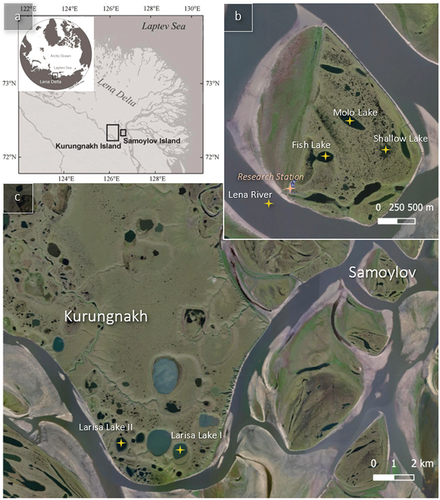
Large thermokarst lakes are typical features of both SAM and KUR (Morgenstern, Grosse et al. 2011; Morgenstern et al. 2013; Muster et al. 2012). Here, we selected six water bodies (five thermokarst lakes and the Lena River) on SAM and KUR, representing conditions of both hydrologically open (e.g., river) and closed (e.g., isolated lake) systems (Table 1). Two of the lakes with the informal names Larisa Lake I (referred to as Oval Lake in previous studies; e.g., in Stolpmann et al. 2022) and Larisa Lake II are located in the southern part of KUR, within late Pleistocene Yedoma deposits. Three additional lakes, namely, Shallow Lake, Fish Lake, and Molo Lake, are located on the much younger deltaic deposits of the Holocene (marine isotope stage 1) on SAM. Previous studies have focused on analyzing the thermal processes in these lakes using data and modeling techniques. Specifically, Sa_Lake_1 (Fish Lake), Sa_Lake_2 (Molo Lake), and Sa_Lake_3 (Shallow Lake) have been extensively studied for this purpose (Boike et al. 2015). The studied water bodies differ in their depths, surface areas, volumes, formation history, and freezing types, as shown in Table 2. Specific characteristics of the cores retrieved from these water bodies (such as coring length, coring date, freeze-up date, etc.) are shown in Table 3.

Table 1. List and aerial image of the investigated water bodies and the retrieved ice cores, their coring depths, and the coordinates.

					Coordinates
Water body		Site	Core	Core depth (m)	LAT	LON
	Shallow Lake	SAM	LD16-BH-6 LD18-BH-3 LD18-BH-9	2.32 2.01 1.63	n/a N72.375169 N72.375011	n/a E126.511306 E126.510853
	Molo Lake	SAM	LD18-BH-4	1.81	N72.377942	E126.497124
	Larisa Lake I	KUR	LD18-BH-12	2.00	N72.295004	E126.204703
	Larisa Lake II	KUR	LD18-BH-11	1.83	N72.297046	E126.118249
	Fish Lake	SAM	LD18-BH-6	1.50	N72.373781	E126.487333
	Lena River	OLE	LD13-BH-1 LD18-BH-8 LD19-BH-2	1.65 1.46 1.76	N72.367764 N72.367545 n/a	E126.467666 E126.468242 n/a

Table 2. List of the investigated water bodies and their morphometric characteristics relevant for freezing.

Water body	Deposit type	Area (km^2)	Volume (m^3)	Depth average/max (m)	Geomorphological water body type	Freezing system
Shallow Lake	HOL	0.026^a	18 800^b	1.0/3.1^a	Polygonal/thermokarst lake	Closed
Molo Lake	HOL	0.042^a	103 600^b	2.6/6.2^a	Thermokarst lake	Closed
Larisa Lake I	PLE	0.421^c	n/d	8.1^c	Thermokarst lake	Closed
Larisa Lake II	PLE	0.323^c	n/d	$\sim$8	Thermokarst lake	Closed
Fish Lake	HOL	0.049^a	106 500^b	3.8/12.7^a	Thermokarst lake	Open?
Lena River	n/a	n/a	n/a	$\sim$25	River	Open

Note. The deposit types refer to the elevated Holocene terrace (HOL) in the east of Samoylov Island and the remnant of a Pleistocene accumulation plain (PLE) on Kurungnakh Island where the investigated lakes are located. The river channels have not been assigned to certain deposit types. We assumed Larisa Lake II to be similar in depth to Larisa Lake I, due to both their similar location and morphometric characteristics.

Sources. ^aChetverova et al. (2017). ^bBoike et al. (2015). ^cMorgenstern, Grosse et al. (2011) and Morgenstern, Röhr et al. (2011).

Table 3. Characterization of the four winters during which the investigated ice cores grew.

Water body	Core	Core depth (m)	Freeze-up date (est.)	Coring date	FDD	Snow depth on core (m)	Snow depth SAM (m)
Shallow Lake	LD16-BH-6	2.32	1 October 2015	19 April 2016	4,709	0	0.22
	LD18-BH-3	2.01	2 October 2017	24 April 2018	4,864	0	0.25
	LD18-BH-9	1.63	2 October 2017	6 May 2018	4,976	0.25	0.28
Molo Lake	LD18-BH-4	1.81	2 October 2015	24 April 2016	4,864	0	0.25
Larisa Lake I	LD18-BH-12	2.00	2 October 2017	7 May 2018	4,988	0.1	0.28
Larisa Lake II	LD18-BH-11	1.83	2 October 2017	7 May 2018	4,988	0.1	0.28
Fish Lake	LD18-BH-6	1.50	2 October 2017	29 April 2018	4,917	0.4	0.31
Lena River	LD13-BH-1	1.65	19 October 2012	20 April 2013	5,160	0.42	0.86
	LD18-BH-8	1.46	19 October 2017	4 May 2018	4,955	0.36	0.28
	LD19-BH-2	1.76	19 October 2018	10 April 2019	4,071	0.2	0.18

Note. “Core depth” is the maximum ice thickness at the time of coring; “FDD” is the freezing-degree days calculated from the estimated day of freeze-up until the day of coring; “Snow cover on core” was observed at the time of coring and “Snow depth at SAM” is from the meteorological station.

Samoylov Island, with the Samoylov long-term observatory established in 1998, provides the closest meteorological record to both our study sites (Boike et al. 2018). Here, summer temperatures can exceed +25°C, and winter temperatures can fall below −40°C (Boike et al. 2013, 2019a, 2019b; Figure 2, Table 4). Typically, air temperatures are positive from June to September and negative from October to May, which roughly corresponds to the ice-covered period for local water bodies (Figure 2). Average annual rainfall is low (169 mm over the period 2002–2018). The snowfall season starts between mid-September and mid-October and generally lasts to late May or early June (Boike et al. 2013; Heim et al. 2022). The snow depth varies greatly, both spatially and temporally, through redistribution by strong winds and is generally relatively thin (~0.3 m; Figure 2, Table 4). The entire delta has been shaped by the interaction between water and permafrost, which has led to a unique hydrological setting with a variety of surface water bodies (Boike, Wille, and Abnizova 2008; Juhls et al. 2021).

Figure 2. Characterization of the four investigated ice-growing periods 2012–13, 2015–16, 2017–18 and 2018–19 by (a) snow depth and (b) air temperature (calculated by average values for each day). Meteorological data were provided by the Samoylov long-term observatory (Boike et al. 2019b).

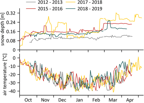
Table 4. Snow depth and air temperature data for the four ice-growing periods (estimated freeze-up until coring), provided by the Samoylov long-term observatory.

Winter	Snow depth (m)			Air temperature (°C)
	Minimum	Average	Maximum	Minimum	Average	Maximum
2012–2013	0.06	0.11	0.13	−39.7	−27.4	−5.5
2015–2016	0.08	0.17	0.23	−39.9	−23.3	−1.8
2017–2018	0.1	0.19	0.32	−43.7	−24.4	1.3
2018–2019	0.11	0.15	0.26	−39.9	−23.4	−3.7

Methods

Sample collection and processing

In total, we drilled ten ice cores from six different water bodies on SAM and KUR during spring expeditions to the Lena Delta in years 2013, 2016, 2018, and 2019 (Overduin et al. 2017; Kruse et al. 2019; Fuchs et al. 2021; Tables 1 and 3). The ice covers were cored with a Kovacs Mark II with an inner diameter of 7.5 or 9 cm, except for the river ice core LD19-BH-2, which was cored with an inner diameter of 7.3 cm. After sampling, all ice cores were described, wrapped, and sealed in plastic tubes and stored in thermally insulated boxes for the transport to Germany, where they were stored frozen until further analysis. Subsampling took place in a climate-controlled room at temperatures of −10°C to −15°C. To determine separation factors ε_ice-water under natural conditions, sub-ice water samples were taken for some of the lake cores as described in the Results section.

During subsampling, we first visually described all ice cores and defined nine different ice types. Based on these ice types, we then generated cryostructural schematics for each core (Figures 3–6). After visual inspection, we sliced the ice cores at 2- to 5-cm intervals. In comparison to earlier studies by Gibson and Prowse (1999), Ferrick et al. (2002), and Taulu (2022), this is the highest sampling resolution performed so far. The subsamples were stored in plastic Whirl-Pak bags. For analysis, they were melted at room temperature. After complete melting, 30 mL of the water was poured by hand from the bags into 30-mL polyethylene narrow-neck bottles for the analysis of stable water isotopes. The remaining water was directly used for measuring electrical conductivity (EC).

Figure 3. Ice morphology, stable isotope signatures, EC, and modeled ice growth (for selected cores) for group I ice cores.

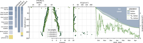
Figure 4. Ice morphology, stable isotope signatures, EC, and modeled ice growth (for selected cores) for group II ice cores.

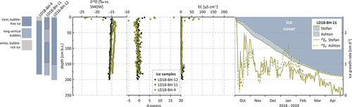
Figure 5. Ice morphology, stable isotope signatures, EC, and modeled ice growth (for selected cores) for group III ice cores.

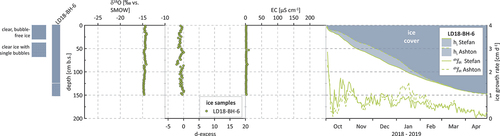
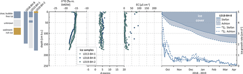
Figure 6. Ice morphology, stable isotope signatures, EC, and modeled ice growth (for selected cores) for group IV ice cores.

Stable water isotopes and EC measurements

Both isotopic fractionation, the partitioning of isotopes during water phase changes, and freeze-out of ions during freezing of water greatly affect the hydrochemistry of ice. Thus, combined stable isotope and hydrochemical investigations of ice bodies can provide a comprehensive understanding of the underlying freezing processes; for example, on water sources, freezing conditions, and system type (e.g., Fritz et al. 2011; Spangenberg et al. 2020).

The samples were measured for their water isotopic composition in the ISOLAB stable isotope facility of the Alfred Wegener Institute Helmholtz Center for Polar and Marine Research in Potsdam, Germany. A Finnigan MAT Delta-S mass spectrometer and equilibrium techniques were used for the online determination of the hydrogen and oxygen isotopic composition, given as δD and δ¹⁸O values relative to Vienna Standard Mean Ocean Water (per mill vs. VSMOW). The measurement accuracy for hydrogen and oxygen isotopes is better than ±0.8 and ±0.1 per mill, respectively (Meyer et al. 2000).

Because the mean annual δ¹⁸O of precipitation is positively correlated with the mean annual air temperature, meteoric waters are isotopically depleted at high latitudes (Dansgaard 1964; Clark and Fritz 1997). The linear relationship between δD and δ¹⁸O in precipitation is described by the GMWL (Global Meteoric Water Line; Craig 1961). The deuterium excess (d-excess) is a second-order parameter reflecting moisture source conditions (such as relative air humidity and sea surface temperature) in precipitation but can also help tracing isotopic disequilibrium processes such as freezing. The d-excess is calculated by (Dansgaard 1964)

(1) $\text{d-excess}=\mathit{\delta D}-8{\delta }^{18}\text{O}$(1)

In a co-isotope plot, δ¹⁸O and δD values of precipitation generally have values that lie on or near to the GMWL (slope S = 8; Craig 1961). Freezing processes are generally characterized by slopes lower than 7.3 (Lacelle 2011). EC was measured with a WTW Multilab 540 device, with an accuracy of ±0.5%, at room temperature and is reported to a reference temperature of 25°C.

Ice growth model

We simulated ice growth on the sampled water bodies between an estimated freeze-up day and the day of coring, comparing two different equations to model ice growth.

As a first-order estimate of ice thickness in the absence of information other than air temperature, the simplified Stefan (1891) equation has been widely used. It is based on the nonlinear relationship between ice thickness h_i and accumulated freezing degree days (FDD):

(2) $h_i=\mathit{\alpha }\sqrt{\mathit{FDD}}$(2)

The value of the coefficient α reflects both the influence of local conditions such as winds and the average snow conditions on ice growth (Comfort and Abdelnour 2013; Murfitt, Brown, and Howell 2018). Michel (1971) proposed typical values for α ranging between 0.7 and 2.7 (U.S. Army Corps of Engineers 2002; Table 5). However, with measured ice thickness, we could calibrate α for each core individually by rearranging Equation (2)(2) $h_i=\mathit{\alpha }\sqrt{\mathit{FDD}}$(2) . To calculate daily ice growth from the estimated freeze-up date until the date of coring, we used Equation (2)(2) $h_i=\mathit{\alpha }\sqrt{\mathit{FDD}}$(2) . The temperature difference between air and surface and the insulating effect of snow are not explicitly accounted for but are parameterized by the fitting parameter α. Any increase of snow cover thickness due to snowfall or wind-driven redistribution of snow are not accounted for, however (Lotsari, Lind, and Kämäri 2019). Consequently, changes to the thermal resistance of snow and their effect on heat transfer between water and air are ignored.

Table 5. Typical values of α, the fitting parameter for calculation of ice thickness using Stefan (Equation (2))(2) $h_i=\mathit{\alpha }\sqrt{\mathit{FDD}}$(2) .

Ice cover condition	α^a
Windy lake, no snow	2.7
Average lake with snow	1.7–2.4
Average river with snow	1.4–1.7
Sheltered small river	0.7–1.4

Note. ^aWith FDD calculated using degrees Celsius and ice thickness in centimeters.

Source. After Michel (1971).

The second ice growth model includes the influences of both changing snow cover thickness and the heat transfer between water and the lower ice surface (Ashton 1989):

(3) ${\rho }_i{L}_f\frac{d{h}_i}{\mathit{dt}}=\left[\frac{\left(T_m-T_a\right)}{\left(\frac{h_i}{k_i}+\frac{h_s}{k_s}+\frac{1}{{\mathit{H}}_{\mathit{sa}}}\right)}\right]-H_{\mathit{wi}}\left(T_w-T_m\right)$(3)

where ρ_i is the ice density, L_f is the latent heat of fusion of ice, T_m is the freezing/melting point of water, T_a is the air temperature, h_i is the thermal ice thickness, k_i is the thermal conductivity of ice, h_s is the snow depth, k_s is the thermal conductivity of snow, H_sa is the heat transfer coefficient at the snow–air interface, H_wi is the heat transfer coefficient between water and ice, and T_w is the temperature of the water at the ice–water interface. For this study, we neglected the last term, assuming that water temperatures varied only negligibly around 0°C at the ice–water interface. To calculate daily ice growth from the estimated freeze-up date until the date of coring, we rearranged Equation (3)(3) ${\rho }_i{L}_f\frac{d{h}_i}{\mathit{dt}}=\left[\frac{\left(T_m-T_a\right)}{\left(\frac{h_i}{k_i}+\frac{h_s}{k_s}+\frac{1}{{\mathit{H}}_{\mathit{sa}}}\right)}\right]-H_{\mathit{wi}}\left(T_w-T_m\right)$(3) and used mean daily air temperatures and the ice and snow thickness of the previous day.

Based on this, we calculated ice growth in centimeters per day and freezing rates for Equations (2)(2) $h_i=\mathit{\alpha }\sqrt{\mathit{FDD}}$(2) and (3(3) ${\rho }_i{L}_f\frac{d{h}_i}{\mathit{dt}}=\left[\frac{\left(T_m-T_a\right)}{\left(\frac{h_i}{k_i}+\frac{h_s}{k_s}+\frac{1}{{\mathit{H}}_{\mathit{sa}}}\right)}\right]-H_{\mathit{wi}}\left(T_w-T_m\right)$(3) ), respectively. Based on calibrated α values, we also used Equation (2)(2) $h_i=\mathit{\alpha }\sqrt{\mathit{FDD}}$(2) to calculate ice growth in centimeters per day and freezing rates for the measured ice thickness.

Based on Equation (2)(2) $h_i=\mathit{\alpha }\sqrt{\mathit{FDD}}$(2) , we used daily modeled ice thicknesses to linearly interpolate the time of freezing corresponding to the sample depths between each ice core sample. For the river ice cores, we then used the estimated times of freezing to compare ice to river water composition (EC, isotope) at the same time. We used river water data from the Lena Water Monitoring Program (Juhls et al. 2020) and the pan-Arctic river sampling program ArcticGRO (Holmes et al. 2021) for comparison.

Model parameterization

For both equations, we start our simulation once a solid ice cover has formed. We estimated this date for each year individually based on optical satellite imagery (Sentinel Hub 2023).

Mean air temperatures, T_a, were taken from the Samoylov data set for both study sites. To account for snow in Equation (2)(2) $h_i=\mathit{\alpha }\sqrt{\mathit{FDD}}$(2) , we assigned an α value representing average snow conditions to each water body, according to categories proposed by Michel (1971; Table 5). Equation (3)(3) ${\rho }_i{L}_f\frac{d{h}_i}{\mathit{dt}}=\left[\frac{\left(T_m-T_a\right)}{\left(\frac{h_i}{k_i}+\frac{h_s}{k_s}+\frac{1}{{\mathit{H}}_{\mathit{sa}}}\right)}\right]-H_{\mathit{wi}}\left(T_w-T_m\right)$(3) , however, requires snow depth data. Because no data on snow depth h_s directly on the ice over winter were available, we used snowfall measurements on the ground as a proxy for the snow depth history. We synthesized snow depth h_s over the ice growth period (i.e., between initiation of freezing and core drilling) out of snowfall (i.e., positive snow depth changes) and measured snow depth on SAM. Until snow depth reached the recorded depth on land at the climate station for each year, we used cumulative positive snow depth changes (i.e., cumulative snowfall). Thereafter, we used measured snow depths at the station (Boike et al. 2019a, 2019b).

Because data for the thermal properties of snow at the study site do not exist, the thermal conductivity of snow k_s required for Equation (3)(3) ${\rho }_i{L}_f\frac{d{h}_i}{\mathit{dt}}=\left[\frac{\left(T_m-T_a\right)}{\left(\frac{h_i}{k_i}+\frac{h_s}{k_s}+\frac{1}{{\mathit{H}}_{\mathit{sa}}}\right)}\right]-H_{\mathit{wi}}\left(T_w-T_m\right)$(3) was estimated using a relationship between conductivity and snow cover density, ρ_s (Yen 1981):

(4) $k_s=2.22362{\left({\rho }_s\right)}^{1.885}$(4)

We tested several snow densities, ρ_s, measured at the Samoylov long-term observatory to identify k_s values that would produce best-fit ice thicknesses for each core individually. The other ice and snow properties (i.e., ρ_i, L_f, k_i, k_s, and H_sa) were considered to be constant over the ice formation period and the same for all years and cores. All values are given in Table 6.

Table 6. Calculated Ashton ice thicknesses vary based on chosen input parameters.

Symbol	Description	Value
ρi	Ice density	917 kg/m^3
Lf	Latent heat of fusion	3.36 × 10^5 J/kg
Tm	Freezing temperature of water	0°C
ki	Thermal conductivity of ice	2.24 W/m°C
Has	Heat transfer coefficient, snow–air interface	20 W/m^2
Hwi	Heat transfer coefficient, ice–water interface	864.6 W/m^2°C
ks → ρs	Snow density
	Freshly fallen snow	0.08–0.16 g/cm^3a
	Damp new snow	0.1–0.2 g/cm^3b
	Settled snow	0.2–0.3 g/cm^3b (SAM, 19 April 2015: 0.267 g/cm^3)
	Typical for the Arctic	0.3–0.33 g/cm^3a (SAM, 26 April 2016: 0.345 g/cm^3)
	Wind-packed snow	0.35–0.4 g/cm^3b (SAM, end of April 2016: 0.4 g/cm^3)
	Very wet snow and firn	0.4–0.8 g/cm^3b
	Extremely wet snow that has been partially melted, refrozen, and compacted	0.5 g/cm^3
	Estimated maximum density of close-packed snow–water mixtures	0.6 g/cm^3a

Note. Calculated Ashton ice thicknesses vary based on chosen input parameters. Some ice and snow properties are considered constant over the entire winter, and the same for each core and year of coring (i.e., ρ_i, L_f, T_m, k_i, H_as, H_wi). Snow properties however are more variable. The thermal conductivity of snow k_s required for Equation (3) was estimated using Equation (4): k_s = 2.22362(ρ_s)^1.885, testing a range of both typical and actually reported values for ρ_s. For example, for Lena River core LD19-BH-2, a value for ρ_s of 0.267 g/cm³, which is within the range of 0.2-0.3 g/cm³ for settled snow (Muskett 2012) and was measured on SAM on April 19, 2015, produced a value of k_s = 0.18 W/m °C which in turn produced the best fit ice thickness of 1.75 m (measured ice thickness 1.76 m). Best fit ρ_s (i.e., those values for ρ_s that produced k_s and resulting ice thickness closest to the measured ice thickness) are given in Table 9.

Sources. ^aAshton (2011). ^bMuskett (2012).

Results

Results are subdivided into four main groups (I to IV), categorized on the basis of maximum water body depths, because the depth of a water body in a continuous permafrost area usually is a critical factor determining the freezing system.

Group I (0–5 m): Shallow Lake

Shallow Lake (maximum depth 3.1 m; Chetverova et al. 2017), the shallowest of the investigated lakes, represents group I (lakes with a maximum depth of less than 5 m). Like most thermokarst lakes on SAM, it formed through the coalescence of several polygonal ponds (Chetverova et al. 2017) and is still in an early stage of this transition. This is apparent from the rough outline, which is a clear remnant of polygonal ground pattern (Table 1; Boike et al. 2015).

The three Shallow Lake cores vary in ice type and year of sampling. LD16-BH-6 (232 cm; 2016) and LD18-BH-9 (163 cm; 2018) have differing ice types, with air bubbles becoming denser and more abundant with increasing depth (Figure 3). LD16-BH-6, with six different ice types (from clear, bubble-free ice; to ice with air bubbles of different density and shapes; to milky ice) across its depth, has the greatest number of ice types occurring in one core (Figure 3). In contrast, core LD18-BH-3 (201 cm; 2018) is completely clear and bubble-free over its entire depth and the only lake ice core of our study comprising only one ice type (Figure 3).

Table 7 provides the summary data of all individual cores. All three ice cores from Shallow Lake show a clear trend of decreasing δ¹⁸O and δD values with depth (Table 7). The lowest δ values occur close to the bottom of the ice, accompanied by a continuous increase in d-excess with depth (Figure 3). The Shallow Lake ice displays the largest oxygen and hydrogen isotope variability of all lake ice cores (SD = 1.9 and 12.6 per mill, respectively; Table 7). In the uppermost ice of core LD18-BH-3, we observe single, very light δ¹⁸O and δD values of −26.2 and −195.5 per mill, associated with higher d-excess and EC values for the same sections of the ice (Figure 3, Table 7). In core LD16-BH-6, from a depth of 2 to 2.23 m, δ¹⁸O and δD values decrease very suddenly, which is accompanied by a sudden increase in EC and a visual change from clear to yellowish ice in the same section of the core (Figure 3).

Table 7. Stable isotope (δ¹⁸O, δD, and d-excess) values (mean [min. to max.]), as well as slopes and intercepts in the δ¹⁸O-δD diagram for all sampled ice cores (δD = slope δ¹⁸O + intercept).

							Slope
Group	Water body	Core	δ^18O (‰ vs. VSMOW)	δD (‰ vs. VSMOW)	d-excess (‰)	EC (μS/cm)	intercept
I	Shallow Lake	LD16-BH-6	−14.5	−117.2	−0.9	2.3	6.5
			[−14.8 to −14.1]	[−119.3 to −114.2]	[−2.2 to 0.1]	[1.6 to 9.8]	−21.9
		LD18-BH-3	−14.7	−117.3	0.5	7	6.8
			[−26.5 to −12.3]	[−196.5 to −101.1]	[−4.8 to 15.5]	[2 to 63]	−17.9
		LD18-BH-9	−14.1	−113.4	−0.9	3.5	6.7
			[−16.1 to −12]	[−126.8 to −100.4]	[−4.8 to 2.9]	[1.9 to 20.8]	−19.1
II	Molo Lake	LD18-BH-4	−14.7	−118.7	−0.7	6.3	6.8
			[−23.9 to −13.6]	[−183.5 to −111]	[−5.1 to 16.6]	[1.9 to 83.5]	−18.9
	Larisa Lake I	LD18-BH-12	−15.4	−124	−0.5	3.6	6.8
			[−17.6 to −14.9]	[−138.6 to −120.5]	[−1.5 to 2.5]	[1.6 to 38.2]	−19.3
	Larisa Lake II	LD18-BH-11	−15.2	−121.9	−0.2	2.9	7.0
			[−23.4 to −14.2]	[−179.9 to −115]	[−1.7 to 7.2]	[1.6 to 13.8]	−14.9
III	Fish Lake	LD18-BH-6	−15.3	−121.4	1.1	20.1	5.8
			[−18.6 to −12.7]	[−142.4 to −104.2]	[−4.7 to 6.4]	[1.9 to 209.5]	−33.4
IV	Lena River	LD13-BH-1	−16	−123.3	4.3	2.9	7.4
			[−17.6 to −14.9]	[−135.8 to −116.1]	[2.8 to 5.8]	[2.2 to 4.7]	−5.2
		LD18-BH-8	−16.5	−126.9	4.8	17	8.3
			[−18.2 to −15.4]	[−141.5 to −118.1]	[3.2 to 6.4]	[3.4 to 93]	9.4
		LD19-BH-2	−16.1	−125.1	4.0	10.5	7.8
			[−18.3 to −14.8]	[−141.9 to −113.2]	[2.6 to 7.1]	[2.8 to 83.8]	1.5

In a co-isotope δ¹⁸O-δD plot, all lake ice cores show slope values between S = 5.8 and 7.0 (Figure 7a), and the Shallow Lake slopes range between S = 6.5 and 6.8. This is lower than those for both the GMWL (S = 8) and the Local Meteoric Water Line (LMWL) for SAM. The latter has a slope of 7.6 for 381 event-based precipitation samples and 7.7 for their monthly means (Spors 2018).

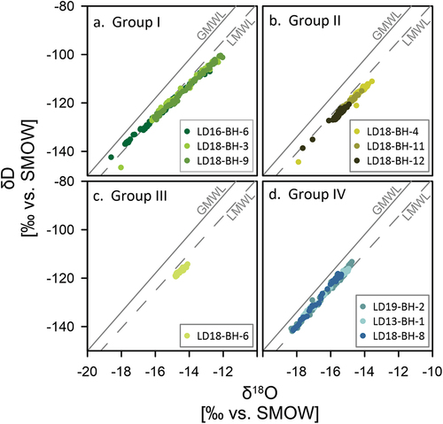
Figure 7. δ¹⁸O-δD plots for (a) Group I: Shallow Lake cores, (b) Group II: Molo and Larisa Lake cores, (c) Group III: the Fish Lake core, and (d) Group IV: the Lena River cores. See Table 7 for regression parameterizations.

For group I, we chose core LD18-BH-9 (total measured ice thickness 163 cm) for the simulation of ice growth, because both core LD18-BH-3 and LD16-BH-6 will be looked at separately in the discussion with cores that share similar snow and ice conditions.

For core LD18-BH-9, both the Stefan Equation (2)(2) $h_i=\mathit{\alpha }\sqrt{\mathit{FDD}}$(2) and the Ashton Equation (3)(3) ${\rho }_i{L}_f\frac{d{h}_i}{\mathit{dt}}=\left[\frac{\left(T_m-T_a\right)}{\left(\frac{h_i}{k_i}+\frac{h_s}{k_s}+\frac{1}{{\mathit{H}}_{\mathit{sa}}}\right)}\right]-H_{\mathit{wi}}\left(T_w-T_m\right)$(3) (referred to as Stefan and Ashton in the following) produce very similar ice thicknesses of 169 cm (Stefan) and 166 cm (Ashton; Figure 3). Maximum growth rates occur on the first day after initial ice cover formation, with values of 3.3 (Stefan) and 2.5 cm/d (Ashton). Within the first ten days of ice growth, growth rates decrease rapidly, which is especially prominent for Ashton, with rates of 0.1 cm/d by 10 October 2017, a week after freeze-up (Figure 3). After this drop, Ashton growth rates stay well below Stefan rates until the end of the year. From late December, however, Ashton growth rates start exceeding Stefan rates until late February. Accordingly, modeled Ashton ice thicknesses stay well below the Stefan thicknesses for most of the winter. Only in the second half of winter, in late February, do both ice growth rates and thicknesses align until the coring date on 6 May 2018 (Figure 3). Minimum growth rate values occur on 1 May for both simulations (−0.02 cm/d), when air temperatures on SAM exceed the freezing point by 1.29°C.

Sub-ice water samples were taken for some of the lake cores, from which separation factors ε_ice-water were calculated using ε_ice-water = δ_ice − δ_water relating the δ values of the last-ice and the associated sub-ice water sample (Table 8). For group I, sub-ice water samples were taken from below cores LD18-BH-3 and LD18-BH-9 and reveal very similar values of ε_ice-water of 2.4 and 2.5 per mill for δ¹⁸O and 15.9 and 16.2 per mill for δD, respectively. Both cores show relatively high EC values for sub-ice water of 246 and 223 μS/cm, respectively (Table 8).

Table 8. δ¹⁸O, δD, d-excess, and EC values for both the last ice formed and for the water below the ice for different water bodies and associated separation factors ε_ice-water for oxygen and hydrogen isotopes.

Group	Water body	Core	Sample type	δ^18O (‰ vs. VSMOW)	εice-water (‰)	δD (‰ vs. VSMOW)	εice-water (‰)	d-excess (‰)	EC (μS/cm)
I	Shallow Lake	LD18-BH-3	Last ice	−16.2	2.4	−127.3	15.9	2.3	23
			Sub-ice water	−18.6		−143.2		5.6	246
		LD18-BH-9	Last ice	−16.1	2.5	−125.8	16.2	2.6	5.8
			Sub-ice water	−18.5		−142.0		6.3	223
II	Molo Lake	LD18-BH-4	Last ice	−14.8	2.5	−118.5	15.7	−0.2	4.5
			Sub-ice water	−17.2		−134.2		3.8	58
	Larisa Lake I	LD18-BH-12	Last ice	−15.8	2.6	−126.8	16.3	−0.8	8.2
			Sub-ice water	−18.4		−143.1		3.8	127.5
	Larisa Lake II	LD18-BH-11	Last ice	−15.5	2.3	−123.8	14.9	0.5	4.5
			Sub-ice water	−17.8		−138.7		3.6	69.4
III	Fish Lake	LD18-BH-6	Last ice	−14.7	2.8	−117.9	18.7	−0.4	3
			Sub-ice water	−17.5		−136.6		3.5	108.3
IV	Lena River	LD18-BH-8	Last ice	−18.2	2.8	−141.1	17.5	4.6	18.7
			Sub-ice water	−21.0		−158.6		9.1	373

Table 9. Results of ice growth simulations for each individual core compared to the actual measured ice thicknesses.

									Difference (measured vs. best-fit calculated ice thickness)
						Calculated ice thickness (best fit)			Stefan		Ashton
Group	Water body	Ice core	hs on top of the ice (m)	hs, Samoylov (m)	Measured ice thickness (m)	Stefan (m)	Ashton (m)	ρs, assumed snow density (g/cm^3)	(m)	(%)	(m)	(%)
I	Shallow Lake	LD16-BH-6	0	0.22	2.32	1.85	1.98	0.6	−0.47	20.3	−0.34	14.7
		LD18-BH-3	0	0.25	2.01	1.88	1.98	0.6	−0.13	6.5	−0.03	1.5
		LD18-BH-9	0.25	0.28	1.63	1.69	1.66	0.4	0.06	3.7	0.03	1.8
II	Molo Lake	LD18-BH-4	0	0.25	1.81	1.88	1.85	0.5	0.07	3.9	0.04	2.2
	Larisa Lake I	LD18-BH-12	0.1	0.28	2	1.9	2.01	0.6	−0.10	5.0	0.01	0.5
	Larisa Lake II	LD18-BH-11	0.1	0.28	1.83	1.9	1.87	0.5	0.07	3.8	0.04	2.2
III	Fish Lake	LD18-BH-6	0.4	0.31	1.5	1.47	1.48	0.345	−0.03	2.0	−0.02	1.3
IV	Lena River	LD13-BH-1	0.42	0.86	1.65	1.21	1.64	0.267	−0.44	26.7	−0.01	0.6
		LD18-BH-8	0.36	0.28	1.46	1.18	1.44	0.267	−0.28	19.2	−0.02	1.4
		LD19-BH-2	ca 0.2	0.18	1.76	1.08	1.75	0.267	−0.68	38.6	−0.01	0.6

Note. Samoylov snow depths are given because they served as input data for the Ashton equation. Measured snow depths on top of the ice at the time of coring are given because they were partly used to reevaluate modeling results in the discussion.

Group II (5–10 m): Molo Lake, Larisa Lakes I and II

Molo Lake, Larisa Lake I, and Larisa Lake II represent group II (lakes with maximum depths between 5 and 10 m; Table 2). Molo Lake, in contrast to many other lakes on SAM, which are small and of irregular shape, has a very smooth outline (Table 1). Beneath its water surface, however, it shows submerged polygonal structures, indicating that it also formed by degradation of ice-rich permafrost and merging of polygonal ponds (Boike et al. 2015). Larisa Lakes I and II both have regular oval shapes as well, which is typical for lakes on KUR (Morgenstern, Grosse, and Schirrmeister 2008).

All three group II lake ice cores show white, milky ice at the top, followed by relatively thick layers of clear, bubble-free ice (Figure 4). Generally, they show little variation of ice types. Core LD18-BH-4 (155 cm) from Molo Lake has the thickest layer of milky ice on top (12 cm) and shows no variation of ice types underneath, with clear, bubble-free ice all the way down to the bottom of the ice. Core LD18-BH-12 (200 cm), with a thinner layer of snow ice on top (5 cm), shows one layer of long vertical bubbles in the bottom part of the ice, and LD18-BH-11 (183 cm), with the thinnest white layer of 2 cm at the top, shows two layers of bubble-rich ice across the core (Figure 4).

The trend of decreasing δ¹⁸O and δD values with depth observed for group I is also evident in the ice from group II, though less pronounced. The cores show slightly narrower ranges in their δ¹⁸O and δD values (SD = 1.3 and 8.9, respectively, Table 7) and no significant increase in d-excess downcore (Figure 4).

The KUR cores have a slightly lighter isotopic composition than all of the SAM cores, except for Fish Lake (Figure 4, Table 7). In the uppermost ice of all three cores of group II, single, very light δ¹⁸O and δD values (e.g., −23.4 and −179.9 per mill for core LD18-BH-11) and relatively high d-excess and EC values for the same sections of the ice could be observed (Figure 4). In a δ¹⁸O-δD plot, the cores plot well below both the GMWL and the LMWL for SAM (Figure 7b). Slope values are between 6.8 (Molo Lake and Larisa Lake I) and 7 (Larisa Lake II) and intercept values are −18.6 per mill (Molo Lake), −19.3 per mill (Larisa Lake I), and −14.9 per mill (Larisa Lake II; Table 7).

For group II, we simulated ice growth simulation using core LD18-BH-11 (Larisa Lake II) as an representative example for water bodies on KUR. For this core (total measured ice thickness 183 cm), the two models produce very similar ice thicknesses of 190 cm (Stefan) and 187 cm (Ashton; Figure 4). Again, modeled ice growth rates are highest on the first day after initial ice cover formation, reaching similar values of 3.7 cm/d (Stefan) and 2.8 cm/d (Ashton). Hence, group I and II water bodies show a similar development of ice growth rates over time: Though Ashton growth rates stay below Stefan growth rates until the end of the year, they exceed Stefan rates considerably thereafter for a couple of months (Figure 4). Accordingly, Ashton ice thicknesses stay well below Stefan thicknesses for most of the winter. In early March, however, both modeled growth rates and thicknesses align for the rest of the ice-growing period; that is, until coring on 7 May 2018, with similar minimum values of −0.02 (Stefan) and −0.03 cm/d (Ashton). Again, these occurred a week before coring on 1 May 2018, when air temperatures were above the freezing point.

For group II, ε_ice-water values are similar for δ¹⁸O across all three lakes (2.5 per mill for Molo Lake, 2.6 per mill for Larisa Lake I, and 2.3 per mill for Larisa Lake II; Table 8). For δD, ε_ice-water ranges from 14.9 per mill in Larisa Lake II to 16.3 per mill in Larisa Lake I. Sub-ice EC varies from 58 μS/cm (Molo Lake) to 127.5 μS/cm (Larisa Lake I). The respective differences between last-ice EC and sub-ice water EC are 53 μS/cm (for Molo Lake), 119 μS/cm (Larisa Lake I), and 65 μS/cm (Larisa Lake II; Table 8). With a mean of 79 μS/cm, these are the lowest differences in EC between last-ice and sub-ice water across all sites.

Group III (>10 m): Fish Lake

Fish Lake with a maximum depth of 12.7 m (Chetverova et al. 2017) is the deepest lake of our study and represents group III (lakes with a maximum depth of >10 m). It yielded the shortest of the lake cores (150 cm). Fish Lake represents an intermediate lake formation stage: In the western part, where the lake is shallow with a rough outline, coalescing polygons are still visible. In contrast, the rest of the lake shows a rather smooth outline (Table 1).

The lake ice is mostly clear and bubble-free and only displays single, round bubbles in the lower 25 cm (125–150 cm; Figure 5).

In contrast to the other lakes, the ice of Fish Lake has an almost uniform isotopic composition with depth (SD = 0.2 and 1.0 per mill, respectively) ranging from −14.8 to −14.1 per mill for δ¹⁸O and from −119.3 to −114.2 per mill for δD (Table 7). Likewise, d-excess values (SD = 0.5 per mill) and EC (SD = 1.2 per mill) are almost uniformly distributed with depth (Figure 5, Table 7). In a δ¹⁸O-δD plot, the Fish Lake ice samples plot well below the GMWL and slightly below the LMWL for SAM (Figure 7c), with a slope value of 5.8 and an intercept of −33.4 per mill (Table 7).

For Fish Lake, the two ice growth simulations produce very similar ice thicknesses of 147 cm (Stefan) and 148 cm (Ashton). Similar to groups I and II, ice growth rates are highest in early winter for both simulations, with maximum values of 2.9 cm/d (Stefan) and 2.3 cm/d (Ashton) on the first day after initial ice cover formation. Within the first two weeks of ice growth, rates decrease suddenly for both simulations (Figure 5). This is especially prominent for the Ashton equation with a value of 0.2 cm/d by 16 October 2017. After this drop, growth rates decrease gradually over the course of winter for both simulations (Figure 5). Similar to groups I and II, Ashton growth rates and thicknesses stay well below Stefan for the first half of winter (Figure 5). Both rates and thicknesses start coinciding again in late February and stay very similar until the coring date, with similar minimum values of 0.23 cm/d (Stefan) and 0.24 cm/d (Ashton) on 29 April.

Across all sites, Fish Lake shows the highest separation factors between water and ice for both δ¹⁸O and δD, with ε_ice-water being 2.8 and 18.7 per mill, respectively. The difference between last-ice EC and sub-ice water EC is 105 μS/cm (Table 8).

Group IV: Lena River

For the Lena River (group IV), in contrast to the lakes, geomorphological characteristics are more difficult to generalize (i.e., deposit type, area, volume, depth). For the Olenyokskaya channel, however, where our cores were retrieved, we assume a maximum depth of 25 m, which is considerably deeper than any of the lakes (Table 2).

The river ice generally shows little variation in ice types. River ice core LD13-BH-1 had already largely broken into pieces in the field, and only two intact core pieces could be obtained (from 0–0.27 m and from 0.40–0.50 m), which were completely clear and free of any air bubbles (Figure 6). For the other river ice cores, the ice is mostly clear and bubble-free as well, except for the top of core LD19-BH-2, which shows a thin layer (ca. 8 cm) of sediment-rich ice (Figure 6).

The isotopic composition is relatively similar among the river ice cores, with mean values of −16 per mill (2012–2013), −16.5 per mill (2017–2018), and −16.1 per mill (2018–2019) for δ¹⁸O and −123.3 per mill (2012–2013), −126.9 per mill (2017–2018), and −125.1 per mill (2018–2019) for δD. According to the isotopic composition, the river ice cores can be divided into three sections: In section one—that is, in the upper ice (from 0 to 0.92 m for LD13-BH-1, from 0 to 0.81 m for core LD18-BH-8, and from 0 to 1.14 m for core LD19-BH-2)—δ values are relatively heavy and display a very narrow range. In cores LD13-BH-1 and LD19-BH-2, this is accompanied by almost constant, relatively low EC values (Figure 6, Table 7).

In the middle sections (from 0.92 to 1.5 m, from 0.81 to 1.3 m, and from 1.14 to 1.55 m), δ¹⁸O and δD values decrease, with shifts from −16.2 to −18 per mill (LD18-BH-8), from −15.3 to −17.5 per mill (LD13-BH-1), and from −16 to −17.9 per mill (LD19-BH-2) for δ¹⁸O, respectively. In the bottom sections, δ values stabilize until the respective maximum depths, at values around −18 per mill for δ¹⁸O (means of −18.0 per mill for LD19-BH-9, −18.1 per mill for LD18-BH-8, and −17.6 per mill for LD13-BH-1).

All three river cores show a strong co-relationship between δ¹⁸O and δD (r² = 0.99, Figure 7d). The samples of the upper ice plot well below both the GMWL (S = 8) and the LMWL (S = 7.7), along regression slopes of 4.7 (LD13-BH-1), 6.8 (LD18-BH-8), and 7.1 (LD19-BH-2). The lower parts of the ice, however, plot along steeper regression slopes of 7.3, 8.2, and 7.8, respectively (Figure 7d). Intercepts are high compared to the lake cores and range between −5.2 per mill (LD13-BH-1) and 9.4 per mill (LD18-BH-8; Table 7).

EC for the river cores ranges between 1.4 and 93.0 µS/cm (Table 7), with means of 5.9, 17, and 10.5 µS/cm for 2012–2013, 2017–2018, and 2018–2019, respectively. For cores LD13-BH-1 and LD19-BH-2, EC stays almost uniformly low over the entire depth of the ice, with slightly increasing values with depth (Figure 6). For core LD18-BH-8, EC was measured for five sections of the ice only (0.12–0.24 m, 0.39–0.48 m, 0.66–0.78 m, 0.92–1.33 m, and 1.42–1.46 m), revealing isolated samples with higher values; for example, 70.2 µS/cm at 0.12 m, 93 µS/cm at 0.66 m, and 46 µS/cm at 1.01 m (Figure 6).

To perform the river ice growth simulation, we selected core LD18-BH-8 (measured ice thickness 146 cm), because core LD19-BH-9 will be discussed separately and LD13-BH-1 has lower core quality. In contrast to the lake ice (of groups I, II, and III), the results of the river ice simulations differ considerably. Whereas Ashton produces a thickness of 144 cm, Stefan yields a much lower ice thickness of only 118 cm (Figure 6). Though both simulations follow the trend of maximum growth rates at the beginning of the ice-growing period, maximum values differ considerably, with values of 3.2 cm/d for Stefan and 5.4 cm/d for Ashton on the first day after initial ice cover formation. In late February, similar to the lake cores, Stefan and Ashton rates align again until the coring date, with similar minimum values of 0.02 for both Stefan and Ashton on 4 May.

Only for core LD18-BH-8 could a sub-ice water sample be retrieved. The separation factors ε_ice-water are similar to group III (Fish Lake) for both δ¹⁸O and δD, with values of 2.8 and 17.5 per mill, respectively (Table 8). Across all sites, the Lena River core shows the highest sub-ice water EC of 373 µS/cm (Table 8). Consequently, with 354 µS/cm, the difference between last-ice EC and sub-ice water EC is highest across all sites.

Discussion

Freezing types

Winter ice covers capture changing water body chemistry during the freezing period. The freezing process and related temperature-dependent isotope fractionation effects modify the ice chemistry. Generally, the freezing velocity is highest during the earliest stages of freezing, steadily decreasing with increasing ice cover thickness. This process is modulated by the development of a snow cover on top of the ice acting as further insulation. Moreover, the chemistry of the ice cover is defined by and can therefore reveal the chemistry of the water, which differs depending on type and geomorphological conditions of the water body.

Closed-system freezing

All ice cores of groups I and II (Shallow Lake, Molo Lake, Larisa Lakes I and II) show decreasing δ¹⁸O and δD values toward the bottom of the ice core. The lowest δ values occur generally close to the bottom of the ice, accompanied by a continuous increase in d-excess.

After freezing, most lakes in our study area are hydrologically closed systems. Firstly, after initial freeze-up, they are blocked from surface recharge. Secondly, because they are located in a continuous permafrost region, they are blocked off from subsurface (i.e., groundwater) recharge by a closed thaw bulb (talik). Usually, the smaller the depth of the lake, the shallower the size of the talik and the lower the volume of water to be refrozen. Hence, in shallower lakes, closed-system freezing will be more likely. During closed-system freezing, heavy isotopes are preferentially incorporated into the ice; the remaining water in closed systems becomes increasingly lighter (Gibson and Prowse 1999, 2002). This generally causes a decrease in the δ¹⁸O and δD values toward the later stages of freezing; that is, the bottom of the ice. Because freezing is a disequilibrium fractionation process, this trend is associated with an increase in d-excess values. Consequently, the last ice formed during closed-system freezing usually displays the lightest isotope composition and the highest d-excess.

Freezing slopes in the δD-δ¹⁸O plot for all cores display slope values between 6.5 (Shallow Lake) and 7.0 (Larisa Lake II), which indicates closed-system freezing under equilibrium conditions (Lacelle 2011).

Because lake water in these Arctic regions derives mostly from precipitation, the concentration of dissolved constituents remains relatively small in the lake ice, which is reflected in overall low EC values. Also, EC values decrease toward the bottom of the ice. This is consistent with closed-system freezing as dissolved ions are excluded from the ice and released into the residual water during the freezing process. As the freezing front moves downwards, it excludes ions from the forming ice and these move toward the bottom of the ice (Shafique et al. 2016). Consequently, in hydrologically closed systems, the EC of ice samples is generally low at the top but increases toward the bottom of the ice, and the highest EC values occur at the water–ice interface. This is the case for all group I ice cores. Complete exclusion of ions from the ice, however, should lead to near-zero EC values, which is not the case. The observed trend suggests a fractionation effect; that is, that the amount of solutes frozen into the ice varies with the concentration of the ions in the remaining water or the rate of freezing.

Though both groups I and II exhibit closed-system freezing characteristics, the depth gradients are far less pronounced in group II than in group I. This can be explained by the shallower water depths of group I and the behavior of isotopes: Heavier isotopes have the tendency to be incorporated preferentially into the ice during freezing and, hence, the isotopic composition of the shrinking water reservoir becomes increasingly lighter (Gibson and Prowse 2002; Lacelle 2011), whereas the d-excess increases. Consequently, a very light isotope composition can be observed in the remaining water.

Open-system freezing behavior of the group III lake

The ice of Fish Lake, in contrast to the other lakes, has an almost uniform isotopic composition with depth and no significant rise in d-excess. The effect of progressively lighter δ values accompanied by increasing d-excess with depth is less pronounced in group II than in group I and almost nonexistent in group III. This is particularly visible when comparing the δ¹⁸O depth profiles (Figures 3–5). EC values do not rise with depth in the core and remain relatively constant, with EC and δ¹⁸O values not being correlated (r² = 0.02). Also, the low regression slope value of 5.76 on a δ¹⁸O-δD plot (Table 7) is below the values that indicate freezing under closed-system conditions (Lacelle 2011).

In hydrologically closed systems, the water budget beneath the ice is restricted, so as winter progresses, only the remaining very light isotopes are integrated into the ice, leading to a pronounced gradient from top to bottom, as can be seen for groups I and II.

The deeper the water body, however, the more likely it is to display open-system freezing characteristics (i.e., to behave geochemically as a hydrologically open system). Constant mixing of water below the ice surface over the course of freezing allows both the reservoir beneath the ice and the ice itself to stay isotopically uniform, meaning almost constant δ¹⁸O and δD values and no significant d-excess rise (Gibson and Prowse 1999, 2002). The deeper a lake, the larger the volume of the remaining water relative to that of the ice, which contributes to this effect. This is why the isotope depth gradient is less pronounced in group II than in group I and there is almost no gradient in group III; that is, in the deepest lake. This is corroborated by the constant EC values at Fish Lake, which do not rise with depth in the core as would be the case for closed-system freezing.

In deep water bodies (i.e., >10 m), the depth alone might lead to this effect while still being blocked off from other water sources. However, with a mean lake depth of 3.8 m (Chetverova et al. 2017), the ratio of ice to water in Fish Lake would be approximately one-third, taking into account the measured ice cover thickness of 1.5 m. Hence, in this case study, only about 35 percent of the total lake water would have frozen at the time of coring. It should be noted that in Boike et al. (2015), the mean/maximum depth of Fish Lake is lower (with 3.0/6.4 m only; corresponding to >50 percent of lake water frozen), potentially missing the deepest part in Chetverova et al. (2017). Hence, this contribution—in both depth scenarios—should have been large enough to lead to a visible closed-system freezing signal in the stable water isotopes, which suggests that Fish Lake tends in fact to act like a hydrologically open system.

Therefore, Fish Lake, in contrast to the other lakes, could not be fully blocked off from water recharge after initial freezing, suggesting a potential second water source to the Fish Lake water budget. This consideration is valid until the coring date only (end of April 2018), and ice growth is expected to continue in May because the ice breakup is in June (Boike et al. 2015). In earlier years, Fish Lake showed a measured and modeled ice thickness exceeding 2 m (Boike et al. 2015). We assume that the large amount of snow (0.4 m) on Fish Lake is responsible for the comparably thin ice cover in 2018.

Lena River as a continuously open hydrological system

The river ice can be divided into three sections: In the upper ice, δ values are relatively heavy and display a very narrow range. In the middle sections, δ¹⁸O and δD values decrease, and in the bottom sections, isotopic values stabilize until the respective maximum depths. This is supported by the regression slopes in a δ¹⁸O-δD plot, where the samples of the upper ice plot well below both the GMWL and the LMWL. The lower parts of the ice, however, plot along steeper regression slopes (Figure 7d). In cores LD13-BH-1 and LD19-BH-2, the change in isotopic composition in the lower part of the ice is accompanied by a slight increase in EC (Figure 6).

In hydrologically open systems with a constant, well-mixed water source underneath the ice cover, the isotopic composition of the ice remains generally constant with depth (Gibson and Prowse 1999), even though isotope fractionation between water and ice might be slightly influenced by the decreasing freezing velocity with time. In contrast to the lakes, the Lena River is a continuously open system, with a decreasing base flow with increasing ice thickness (Juhls et al. 2020).

For the Lena River, however, the ice shows a clear division into sections of different isotopic signatures and does not show constantly decreasing δ values downcore as expected for a hydrologically open system (compare Fish Lake). The observation that the ice cover of the Lena River shifts from near-constant δ¹⁸O and δD values in a relatively heavy range to a section of constant values in a lighter range suggests either a change of water sources underneath the ice cover or disruption of the ice cover through aging processes over the course of the winter. However, changes in isotopic composition are not abrupt enough to suggest mechanical disruption of the ice cover.

In the case of temporally varying water sources, the isotopic composition of the water would change depending on the changing relative contribution of individual water sources. Hence, shifts in isotopic composition and EC with depth in the ice of a hydrologically open system may reflect changing water sources underneath the ice cover over winter.

In the Lena River, the water chemistry is defined by sources of water from the catchment. Over the course of winter, the Lena River is influenced by two major freshwater sources: Rainwater is the dominant water source until freeze-up, and this influence decreases gradually below the ice in the first half of winter. In the second half of winter, subsurface water remains as the only significant natural water source (Juhls et al. 2020). The third major source, snowmelt, becomes important only when the melting starts, and this is associated with the period of breakup and decay of the ice cover. This latter source can be largely ruled out taking into account that the coring period in spring is well before the melting starts.

The upper, isotopically heavy section of the river ice grew during the first half of winter, with high δ values indicative of meteoric origin (Juhls et al. 2020; Spangenberg et al. 2020). However, because the freezing velocity decreases from top to bottom, it is not only the river water source but also fractionation during freezing that affects the isotopic composition. Hence, the very light δ¹⁸O values of the first, topmost ice in core LD18-BH-8 and LD19-BH-2 may be explained by rapid freezing rates that typically occur at the beginning of the ice-growing period at reduced fractionation (Ferrick et al. 2002; Figure 6). These secondary processes overprint the precipitation signal (if precipitation was the source).

The decreasing isotopic composition in the middle sections of the river ice likely reflects the gradual decrease in δ¹⁸O values of Lena River water due to a lower rainwater contribution. The bottom sections, with relatively light and stable δ values, could reflect the stabilization of river water values at around −21 per mill in early March, characteristic for a subsurface water contribution (Juhls et al. 2020).

An increase in EC in cores LD13-BH-1 and LD19-BH-2 is consistent with a change from rain to subsurface water; that is, from low to higher EC levels in the river water. Generally, low EC for the river ice cores, with slightly rising values with depth, suggests open-system freezing and the addition of a secondary water source rich in ions in late winter (Figure 6). Isolated samples with higher EC values in core LD18-BH-8 were often observed near breaks of the core, which could be the effect of freezing of river water onto the core at a breakpoint in the core during recovery.

Even though temporal variations in fractionation between ice and water can affect both the isotope composition and EC, we assume changes in sub-ice water chemistry to be transferred to the ice, reflecting ice growth under open-system freezing conditions. In summary, river ice is a good indicator for the sources of the contributing waters and their changing relative contributions, especially evident in late winter.

Source water variability

Precipitation intermittency and evaporation

The water chemistry of shallow water bodies can be strongly affected by precipitation events just before freeze-up. As a consequence, different isotopic signatures or EC of the water bodies at the onset of freeze-up can result in strong interannual differences of the ice cover chemistry. This effect can explain the lighter isotopic composition in the Shallow Lake ice grown in 2015–2016 compared to the Shallow Lake from 2017 to 2018. Core LD16-BH-6 (δ¹⁸O between −18.6 and −12.7 per mill, mean −15.3 per mill) has a slightly lighter isotopic composition compared to the cores LD18-BH-3 (δ¹⁸O between −16.2 and −12.3 per mill, mean −14.2 per mill; excluding the upper four samples or 15 cm of ice, which we defined as snow ice) and LD18-BH-9 (δ¹⁸O between −16.13 and −12 per mill, mean −14.1 per mill). Additionally, secondary moisture sources (i.e., local open water bodies) may contribute to the isotopic composition of precipitation (Bonne et al. 2019), leading to low d-excess precipitation events. The relatively light isotopic composition of the core LD16-BH-6 could point to a strong (isotopically light) precipitation event before freeze-up.

Shallow and small water bodies are sensitive to evaporation. Evaporation under non-recharge conditions is accompanied by both an enrichment in δ¹⁸O and δD as well as a systematic decrease in d-excess (Surma et al. 2015). Hence, δ¹⁸O and δD values in an evaporative water body are significantly higher and d-excess values are significantly lower than those of local precipitation.

For the observation periods of JJA (June, July, August) and SON (September, October, November) 2015, the mean seasonal isotopic composition of precipitation at Samoylov station were −16.0 and −23.4 per mill for δ¹⁸O and 6.6 and 8.8 per mill for d-excess, respectively (Spors 2018). δ¹⁸O values for the uppermost Shallow Lake ice samples, being closest to the isotopic composition of the water just before freeze-up, are significantly more positive; for example −12.8 per mill for LD16-BH-6 and LD18-BH-3 (that is, below the first 15 cm of this core, which has been defined as snow ice; see section on snow) and −12.6 per mill for LD18-BH-9. D-excess values of the first ice are relatively low, with values of −4.7, −4.0, and −3.4 per mill, respectively. Both higher δ¹⁸O and lower d-excess values compared to mean seasonal precipitation at the station for the time before freeze-up may indicate evaporative loss under non-recharge conditions for Shallow Lake.

In summary, shallow lakes are most prone to the influence of evaporation- or precipitation-related change of the water reservoir prior to freezing. They are generally characterized as hydrologically closed lakes, where the fractionation during freezing and downcore isotopic gradients are strongest. Closed-system freezing also takes place in other, deeper lakes. However, because precipitation intermittency and evaporation do not influence these to a similarly strong degree, they reflect long-term meteorological conditions rather than short-term events.

Snow

For four of the lake cores (LD18-BH-3 from Shallow Lake, LD18-BH-4 from Molo Lake, LD18-BH-11 from Larisa Lake II, and LD18-BH-12 from Larisa Lake I), we observed very light δ¹⁸O and δD values in the top parts of the ice, correlating with relatively high d-excess and EC values for the same increments (Figure 8). In addition, in all but one of these cores (LD18-BH-3) we observed milky white ice at the top (Figure 8b).

Figure 8. Isotopic snow ice signals (a) on a δ¹⁸O-δD plot and (b) in the upper 20 cm of core LD18-BH-4 (Molo Lake). Note the reflection of the isotopic snow ice signal (i.e., light δ¹⁸O values in the upper ice) in the visual ice characteristics (milky white snow ice).

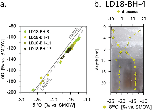
This can be best explained by snow events early in the ice growth season that are likely to affect the top layer; that is, the first, topmost ice on top of lakes and rivers in our study area. When the weight of the snow layer presses the still thin ice during early freezing below the water level, water and snow may mix at the surface and form a layer of snow ice above the actual first ice (Jeffries, Morris, and Duguay 2012). The white and milky color of the ice is likely characteristic for snow ice.

Because the snow ice isotope signals are often accompanied by high EC values, this further supports heterogeneous ice development in the early stage of freezing. Snow usually has a low EC, but because snow ice is formed in contact and during mixing with underlying lake water, EC values in snow ice are usually high. This also suggests that the observed geochemical signature is not associated with snow alone.

The δ¹⁸O-δD regression slope values of these cores are lower than that of the GMWL but in close agreement with the slope of the closest LMWL (Figure 8a). Although this could indicate a meteoric origin (i.e., precipitation), a freezing slope is influenced by the freezing conditions as well and if snow becomes part of the ice, the upper parts of the ice plot very close to the GMWL on a δ¹⁸O-δD plot, as observed for the four lake cores mentioned above.

The light δ¹⁸O values in the first ice/top layer ice, the high d-excess values, relatively high EC, and visual appearance of the ice are thus interpreted as indicative of the formation of snow ice on these water bodies in the early stage of freezing.

Potential hydrological subsurface connections

Effectively blocked off from additional water sources over winter, we usually expect thermokarst lakes in our study area to exhibit closed-system freezing characteristics (i.e., decreasing δ¹⁸O and δD values and increasing d-excess with depth), as observed for lakes of groups I and II.

However, in the ice of Fish Lake (group III)—the deepest of the investigated lakes by depth—both isotopic composition and EC stay almost constant over the entire depth of the core (Figure 5). Also, the low regression slope value of 5.76 in a δ¹⁸O-δD plot does not represent a clear freezing slope of a closed-system freezing, with δ¹⁸O-δD regression slope values between 6 and 7.3 suggesting freezing under equilibrium conditions (Lacelle 2011).

Both the almost uniform isotopic and EC values of the ice with depth and the low regression slope suggest open-system freezing. Moreover, the constant isotopic composition points to a hydrologically open system, where the water source beneath the ice remains the same throughout the winter (i.e., the isotopic composition of the underlying water does not change significantly) and therefore isotopic composition and EC values remain stable over the entire depth of the ice (Gibson and Prowse 1999). It is speculated that later recharge underneath the ice or a connection to another uniform, isotopically similar water source could be explanations, though there is no further evidence for this assumption. Though the lake is deep enough to develop a talik, groundwater recharge from surrounding soils would be too slow to have significant impact on the isotopic composition of a seasonal ice cover and would also be reflected in a potential EC rise with depth, which is not observed in Fish Lake.

Separation factors between sub-ice water and last ice formed

Experimentally determined separation factors ε_ice-water between ice and water in freshwater systems range between 2.8 and 3.1 per mill for δ¹⁸O (Suzuoki and Kimura 1973) and from 17 to 21 per mill for δD (Arnason 1969), respectively. To determine separation factors ε_ice-water under natural conditions, sub-ice water samples were taken for some of the lake cores (Table 8). For all sites, the last ice in each core is enriched in heavy isotopes as compared to the sub-ice water by nearly constant separation factors ε_ice-water (Table 8; min. 2.3 per mill, max. 2.8 per mill, mean 2.5 per mill for δ¹⁸O and min. 14.9 per mill, max. 18.7 per mill, mean 16.5 per mill for δD). Hence, the calculated ε_ice-water are slightly lower but close to those experimentally determined for equilibrium fractionation, which is in line with findings by Taulu (2022) in the Athabasca River Basin, Canada. Hence, the ice is a reliable indicator of the isotopic composition of source water, especially in late winter when ice growth is slowest (Gibson and Prowse 1999).

The largest differences between last-ice EC and sub-ice water EC for the Lena water–ice pair point to the seasonality of the Lena water; that is, the high influence of subsurface water in the second half of winter. This was supported by Juhls et al. (2020), who identified subsurface water as the main Lena water source in spring at the time of coring. Relatively high EC differences in group I (Shallow Lake) may be due to the shallow depth of the water body and possible interactions between sediment and the residual water below the ice at the end of winter. Conversely, relatively low EC differences between ice and water for groups II and III may point to no or only little interaction between sediment and residual water.

Ice growth models

Ice growth is controlled not just by water body chemistry but by external factors as well such as mechanical disruption and snow events during freeze-up, snow cover development, and winter weather (e.g., winter air temperatures). In the following subsections, we target how well different events controlling ice growth are captured by the two models, Ashton and Stefan.

Snow insulation effect

The Stefan and Ashton equations use input parameters of different resolutions. Ashton, most importantly, considers the effect of snow and its properties in the form of p_s (density of snow), k_s (thermal conductivity of snow), and h_s (snow cover thickness). So, firstly, the comparison between both models gives information about whether adding the respective data actually causes an improvement in predicting ice thicknesses.

Between Ashton and Stefan, simulated ice thicknesses and resulting growth rates differ over the first half of winter (Figures 3–5) but start to align in late February until the respective coring dates. The differences in early winter can be explained by the different resolution of input parameters. Both models account for changing winter air temperatures (in the form of FDD for Stefan and T_a for Ashton, Equations (2)(2) $h_i=\mathit{\alpha }\sqrt{\mathit{FDD}}$(2) and (3(3) ${\rho }_i{L}_f\frac{d{h}_i}{\mathit{dt}}=\left[\frac{\left(T_m-T_a\right)}{\left(\frac{h_i}{k_i}+\frac{h_s}{k_s}+\frac{1}{{\mathit{H}}_{\mathit{sa}}}\right)}\right]-H_{\mathit{wi}}\left(T_w-T_m\right)$(3) )). However, whereas Stefan assigns a constant alpha value that only represents whether the water body as a whole is influenced by snow at all, Ashton also takes into account what properties the snow has (i.e., ρ_s and k_s) and how the snow cover develops over time (h_s). Hence, slower ice growth in early winter for Ashton captures that in early winter, when the ice is still thin, the snow cover has a high relative insulation effect. Similar results for both equations toward the end of winter, in turn, capture an increasing insulation effect of the thickening ice cover itself, which reduces the effect of insulation by snow alone (Bengtsson 2012).

Snow ice

For most cores, the Ashton equation produced ice thicknesses close to measured values when using values of ρ_s reported for the study site (Table 9). For cores that had no or only a very thin snow cover on top of the ice, however, typical values of ρ_s did not produce realistic ice thicknesses (Table 9). There could be several reasons for this. Firstly, although we determined thermal conductivity of snow, k_s, based on typical density values for snow, ρ_s, alone, the thermal conductivity of snow is not solely a function of its density but also changes with age or temperature, though the temperature effect is considered to be small (Yen 1981). Still, snow densities change continuously from the moment of the first snowfall until snowmelt in spring, including possible rainfall events and submergence of the snow cover (Duguay et al. 2006).

Secondly, untypically high values might point to the formation of high-density snow ice or slush on top of the ice. Though slush and snow ice are more commonly observed on rivers, they can also appear on large lakes where ice formation, especially in the early stages of freezing, is more dynamic than that on smaller lakes (Jeffries, Morris, and Duguay 2012). Because of the differences in air content and crystal structure, the density and thermal properties of snow ice and the underlying secondary ice differ (Greene and Outcalt 1985). Snow ice forms when water that seeps into the bottom of the snow causes the snow to densify and reach values of up to 600 kg/m³ (Ashton 2011). This aligns with the values for ρ_s that did produce good-fit ice thicknesses; that is, 500 kg/m³ (LD18-BH-4 and LD18-BH-11) and 600 kg/m³ (LD16-BH-6, LD18-BH-3, and LD18-BH-12).

The depth profiles of cores LD18-BH-3 (Shallow Lake) and LD18-BH-4 (Molo Lake), as well as those for the two KUR cores, show high EC values in the top ice. High ion, isotopically light lake water points to the involvement of snow rather than flooding alone, which would mean mixing with isotopically heavy lake water (Jeffries, Morris, and Duguay 2012). The milky white ice at the top of these cores (except LD18-BH-3; Figures 3 and 8b) supports that high ρ_s values of up to 600 kg/m³ reflect the formation of snow ice in the early stages of freezing.

Bottom fast ice/doming effect in Shallow Lakes

For core LD16-BH-6, the Ashton equation did not produce realistic ice thicknesses either (Figure 9). In contrast to the lake cores discussed previously, however, even very high-density values still underestimate ice growth considerably (1.98 m with ρ_s of 600 kg/m³ and measured ice thickness of 2.32 m; see Figure 9b).

Figure 9. Results of the ice growth simulations for core LD19-BH-2 (a) and core LD16-BH-6 (b). The cores were chosen to discuss (a) the underestimation of river ice growth by Stefan and (b) the effect of using snow data of different resolutions in the Ashton equation.

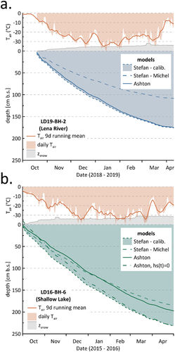
The main reason for this inaccuracy is likely to be that in our study, snow data from a landlocked snow station on Samoylov were used to draw conclusions on ice formation on nearby reservoirs. However, snow covers on reservoirs tend to be significantly less than that at nearby ground stations. Wind redistributes snow, which leads to a thinner and denser snow layer over reservoirs than over land (Sturm and Liston 2003). For instance, the average fraction between the snow depth measured over lake ice and the snow depth measured over land at the Barrow weather station in Alaska was observed to be 52 percent (T. Zhang and Jeffries 2000). This suggests that for core LD16-BH-6, using snow data measured at the landlocked station might suggest an insulating effect that did not actually exist on the water body. Indeed, using values of h_s = 0, instead of SAM snow depths, produces an ice thickness of 2.33 m, which is very close to the measured ice thickness of 2.32 m (Figure 9b).

The reason for this particular core being snow-free may lie in the transitional stage of Shallow Lake. In our study area, the merging of small ponds causes the formation of larger water bodies (Langer et al. 2015). Lakes with depths greater than 2 m develop floating ice, which means they remain unfrozen at the bottom throughout the winter (Jeffries, Morris, and Duguay 2012; Muster et al. 2017). Shallow ponds with water depths of less than 1 m, however, usually develop bedfast ice (Langer et al. 2011).

Because it is in an early stage of transitioning from a pond into a lake (Chetverova et al. 2017), Shallow Lake, at least in parts, would have frozen to the bed. The formation of bedfast ice, in turn, leads to an increase in volume and the resulting hydraulic pressure may cause the formation of a dome in the center of the water body. This part of the lake is especially exposed to wind and usually remains snow-free for the rest of the ice-growing period. Therefore, the fact that assuming no snow produces a realistic ice thickness for core LD16-BH-6 suggests that it has been cored in such a location (in contrast to the other two Shallow Lake cores that were cored closer to the shore where the snow is redistributed to from the center by winds). This is supported by both field book entries and photography from the coring site that indicate that this core was retrieved from the central, deep part of the lake, which might have been free of snow for the most part of winter due to its exposition.

Although the data record provides evidence for considerable snow fall on Samoylov Island for the winter of 2015–2016, snow densities of above 600 kg/m³ point to a doming effect and a resulting lack of a snow cover in the central part of Shallow Lake.

River ice growth

The comparison between models and observed ice thickness gives information about how well the models fit overall. In contrast to the lake cores, for the river ice, Ashton and Stefan do not produce similar ice thicknesses (see Figure 9a for exemplary river core LD19-BH-2). Whereas Ashton produces thicknesses very close to the measured ice thicknesses, the Stefan model produced much lower ice thicknesses of only 1.21, 1.18, and 1.08 m, respectively (Figure 9b for Shallow Lake core LD16-BH-6).

Stefan

There could be several reasons for the underestimation of river ice growth by the Stefan equation. Firstly, as discussed before, our use of the Stefan model includes snow effects only as part of the fitting coefficient, α. Generally, α is therefore inversely related to snow thickness. For example, if α includes the effects of snow cover above and frazil ice (an ice type that forms in turbulent flow conditions and is primarily found in rivers; Jeffries, Morris, and Duguay 2012) below the ice, then the value of α becomes larger when snow and frazil ice become part of the ice sheet and smaller when snow cover and frazil ice insulate the ice (Yoshikawa, Watanabe, and Itoh 2014). In this study, the proposed value for “average river with snow” of 1.7 (Table 5) led to an underestimation of ice growth. This suggests that the categories proposed by Michel (1971) are not sufficient for the Lena River or that snow and frazil ice/slush play a more important role in our study site than his categorization allows.

This is supported by Yoshikawa, Watanabe, and Itoh (2014), who found that the Stefan equation is inapplicable under certain conditions. According to them, it is not possible to assign a constant value to the coefficient α when there is significant snowfall, change in the volume of snow cover due to wind, or change in frazil ice concentration due to flowing water. Moreover, because snow ice, aufeis, and/or slush formation are generally important features of river ice (Jeffries, Morris, and Duguay 2012), neglecting them would have a potentially important impact on river ice simulation.

In a simulation of river ice growth at the Pulmanki River by Lotsari, Lind, and Kämäri (2019), the least correspondence (underestimation) between the estimated Stefan thickness and observed ice thicknesses was during the years that had the thinnest snow covers and the thickest maximum and average ice covers. This also aligns with the results of our study: out of the three river cores, LD19-BH-2 had the least correspondence between Stefan and measured ice thickness (1.08 m vs. 1.76 m), for the thickest ice (1.76 m compared to 1.65 and 1.46 m, respectively), and for thinnest snow cover (ca. 0.2 m compared to 0.42 and 0.36 m for 2013 and 2018, respectively). Lotsari, Lind, and Kämäri (2019) suggested that this underestimation is at least partly due to the fact that the Stefan equation does not account for snow ice formation.

The application of the Stefan model does not necessarily lead to an underestimation of river ice growth. Ma, Yasunari, and Fukushima (2002), for instance found an overestimation of river ice thickness for their four observation sites located along the Lena River using Stefan. They attributed this to snow cover on the surface of the river ice not being considered. The river reaches selected (Yakutsk, Olekminsk, Vitim, and Kirensk) are located upstream and midstream along the Lena River where freezing begins later, in late November, and thawing earlier compared to downstream, where thawing occurs in late June (Ma and Fukushima 2002). This means that the ice downstream has a longer growth period. Accordingly, Ma, Yasunari, and Fukushima (2002) observed a trend of deepening ice along the river.

The underestimation of river ice growth by Stefan points to the fact that neglecting events like snow ice/slush formation, which are especially prominent on rivers, makes this equation difficult to apply to Lena River ice growth. Additionally, contrasting results for different regions of the river suggests that snow alone is not enough to explain problems with Stefan model estimation of ice thickness.

Ashton

Whereas Stefan significantly underestimates river ice thicknesses, Ashton produces values that are very close to the actual measured river ice thicknesses (1.64 m for LD13-BH-1, 1.44 m for LD18-BH-8, and 1.75 m for LD19-BH-2, with measured ice thicknesses of 1.65, 1.46, and 1.76 m, respectively, when using reported average ρ_s values of 0.267; Table 9). The reason for this is likely to be that Ashton incorporates properties of ice and snow cover.

Our results align with F. Zhang, Li, and Lindenschmidt (2019), who used the Ashton equation to determine the ice thicknesses along the Slave River in Canada. Their method also resulted in better thickness estimates than the Stefan equation. However, whereas we determined thermal conductivity of snow based on typical density values for snow alone, they developed a model for snow wetness determination that was used to define the thermal conductivity of snow. They then also used direct measurements, gathered during the winter of 2014–2015, to calibrate the model. Without the possibility of continuous sampling, we assume that high thermal conductivities mainly result from high densities. The fact that this approach produced thicknesses very close to the measured ice thicknesses suggests that ρ_s is indeed the dominant factor for thermal conductivity of snow.

Comparison of river water and ice composition

Firstly, we compared the values of river ice and river water in terms of EC and isotopes. The difference between river water and ice core EC ranges from around 150 to 440 µS/cm and generally increases over the winter (Figure 10a). Plotted as a function of ice growth rate, a relatively smooth exponential decrease in solute exclusion, measured as EC difference, is observed (Figure 10b). The more rapidly the water freezes at the base of the river ice, the less effectively solutes are excluded from the forming ice matrix and the lower the difference between river water and ice ECs. This stands in contrast to the relatively constant isotope fractionation over time and with respect to ice growth rate (Figure 10c, d). It also suggests that the river ice in our study contains a record of its own growth rate, provided that something is known about the water from which it derives. In our case, the data suggest that knowing the difference between EC in the ice and the river provides a means of relatively accurately (to within a few millimeters per day) reconstructing the growth rate. This also indicates how valuable our high-resolution (2-cm) subsampling of ice cores is, especially when comparing this to other studies generally employing lower resolution (i.e., 5 to 10 cm; Gibson and Prowse 1999; Taulu 2022). For the Lena River ice core LD19-BH-2, freezing periods interpolated to the 2-cm subsampling were less than one day and up to thirteen days per sample (mean = 2.2; median = 2 days). Finer subsampling, using ablation or continuous flow sampling techniques and connected to higher frequency sub-ice water sampling than our roughly twice-weekly sampling, may even provide more highly temporally resolved information on processes affecting ice cover formation and its connections to environmental forcing and water body characteristics.

Figure 10. Differences between river water and ice chemistry. The time of freezing for ice cores was estimated using the ice growth models of Ashton. Ice chemistry is compared to water samples from the Lena Monitoring (+) and ArcticGRO (o) programs. (a) The difference in electrical conductivity (i.e., salt exclusion) over the 2018–2019 winter, (b) the same difference in EC plotted as a function of ice growth rate, (c) separation between river water and ice δ¹⁸O over the winter ice growth period (ε_ice-water = δ_ice − δ_water; see Gibson and Prowse 2002), and (d) variation of the same fractionation values (excepting the upper six ice core samples) as a function of estimated ice growth rate.

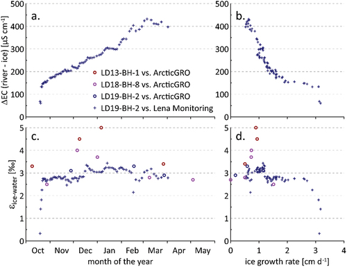
In early winter, when isotope values (whether river water or ice) are heavier, the data depart from the equilibrium fractionation line, which is especially prominent for the first four ice values (Figure 10). This corresponds to a threshold ice growth rate of ca. 3 cm/day. Below this threshold, the classical equilibrium fractionation with a separation factor ε_ice-water of ca. 2.8 to 3.1 per mill between water and ice is reached (Suzuoki and Kimura 1973). Hence, similar to observations for winter ice–water pairs from Liard and Mackenzie rivers (Gibson and Prowse 2002), separation factors for the Lena River are close to theoretical equilibrium fractionation (Figure 11, Table 8). In spring, however, at the slowest ice growth rates, the data fall slightly below the equilibrium fractionation line (Figure 11), as also observed by Gibson and Prowse (2002).

Figure 11. The stable oxygen isotope concentration in river ice (ice core LD19-BH-2) vs. interpolated values for sub-ice river water during ice growth. The linear fit is for congelation ice samples only (i.e., without the uppermost four ice core samples, gray open circles) and has the form: δ¹⁸O_ice = 0.93 δ¹⁸O_water + 1.54 (n = 75, R² = 0.96).

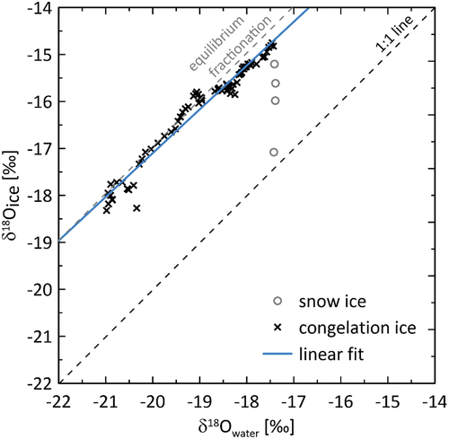
Small separation factors may be explained by rapid freezing rates that typically occur at the beginning of the ice-growing period and are expected to reduce fractionation (Gibson and Prowse 1999; Ferrick et al. 2002). Also, as discussed earlier, the upper ice, especially on rivers, is often influenced by the formation of snow ice (e.g., Jeffries, Morris, and Duguay 2012) for which light isotopic values are characteristic.

After initial ice formation, freezing is less likely to be disturbed, especially after the ice is covered with snow. Congelation ice can form (clear, coarse-grained often columnar ice, which, in contrast to snow ice, has been found to hold systematic isotopic patterns with isotope offsets close to the equilibrium ice–water fractionation; Gibson and Prowse 2002). Gibson and Prowse (2002) found that vertical distributions of stable isotopes in river ice cores were generally characterized by the presence of an upper layer of white, polycrystalline ice that is depleted in the heavy isotopes due to incorporation of snow and an underlying zone of congelation ice. The slowest freezing rates typical for the end of winter are generally accompanied by the highest fractionation between water and ice (Ferrick et al. 2002). Therefore, lower separation factors for the lowest δ¹⁸O values may point to melting at the very end of the winter.

Fractionation as a function of time

To examine the difference between river water isotope values, we used the modeled time of freezing to compare ice and river water samples directly. Reference water samples were provided by the pan-Arctic river sampling program ArcticGRO (Holmes et al. 2021) and by the Lena River Monitoring Program (Juhls et al. 2020).

The degree to which water isotopes fractionate into ice depends on the freezing rate and velocity (Gibson and Prowse 1999; Ferrick et al. 2002), with rapid freezing rates reducing isotopic fractionation and slower freezing rates leading to higher fractionation (Ferrick et al. 2002). Consequently, due to the changing source water contributions to the Lena River over winter, isotopic composition of the river ice changes with depth or time. The individual isotopic composition of the respective source water, however, should not affect the ice–water separation, because the river ice is isotopically enriched relative to the respective water source, in the case of equilibrium freezing by a separation factor of about 3 per mill for δ¹⁸O (Gibson and Prowse 2002).

For the investigated river water–ice pairs, the inferred fractionation ranges between 0.3 and 5 per mill for the set of all samples for freezing times inferred from both the Ashton and Stefan models (Figure 10). Early winter has a consistently lower fractionation (<3 per mill) until mid-December, after which values lie above 3 per mill and slowly decrease until spring. There is not much variability over the year for the Lena Monitoring samples (fractionation of 2 to 3.5 per mill); separation factors are actually close to equilibrium values of 3 per mill in most cases, with the exception of the uppermost ice samples, which, as discussed previously, probably reflect snow/snow ice.

Comparison of Lena River ice isotope composition to the ArcticGRO data, however, ranges between 2.5 and 5 per mill. This may be the result of the spatial offset between river water and ice coring locations: ArcticGRO samples were collected in Zhigansk, which is located about 800 km upstream of the river mouth and about 220 km upstream from Samoylov Island, where both Lena Monitoring data and ice cores were collected. Consequently, the travel time and input/removal of water underneath the ice might cause this effect.

Fractionation as a function of freezing rate

The ArcticGRO data show that fractionation generally increases with ice growth rate for growth rates between 0 and 1 cm/d (from 2.7 to 5 per mill), with an outlier at early winter rapid ice growth of 1.5 cm/d (2.5 per mill) that may be affected by snow (Figures 10c, 10d).

This trend is not seen in comparison with Lena Monitoring data: Here, fractionation rates are variable at low ice growth rates but mostly high (around 3 per mill); above 1.6 cm/d isotope fractionation is relatively uniform at around 2.6 per mill (Figures 10c, 10d). High separation factors correspond with intermediate freezing rates between 0.5 and 0.9 cm/d (Figure 10d).

Excluding snow ice, equilibrium fractionation was observed from the very beginning to the very end of the ice-growing period, which corresponds with the highest and slowest calculated freezing rates, respectively.

This may be connected to the spatial offset between river water and ice core locations. The fact that there is a correlation of changing isotopic composition in the river ice (mid-winter) and high separation factors (between December and January; at intermediate freezing rates) between water samples taken in Zhigansk and ice grown opposite SAM suggests that the change from rain- to subsurface water does increase the ice–water separation between these two places. The remaining rainwater is being removed from underneath the ice and the water level is gradually lowered, causing the lowest annual river discharge (Juhls et al. 2020). The gradual removal of remaining rainwater leads to an exchange of dominant water sources earlier in Zhigansk and later downstream, toward the outlet.

Transfer of river water signals into the ice

To further investigate the timing of the change in river water sources, we used the Stefan equation to calculate freezing periods for individual river ice core samples. We then compared the estimated times of freezing for each river ice sample with river water samples from the same year to investigate isotopic fractionation between ice and water for three different ice-growing periods (i.e., 2012–2013, 2017–2018, and 2018–2019; Figure 12). Reference water samples were again provided by ArcticGRO (Holmes et al. 2021) and the Lena River Monitoring Program (Juhls et al. 2020).

Both water and ice values show a relatively heavy isotopic composition shortly after (estimated) freeze-up. After freeze-up, the isotopic composition stays relatively stable before decreasing in the second half of winter and stabilizing again in early March (Figure 12).

Figure 12. River ice δ¹⁸O values for all three river ice cores compared to reference data from the respective years (2012–2013, 2017–2018, and 2018–2019) provided by ArcticGRO and the Lena Monitoring Program (the latter for 2018–2019 only).

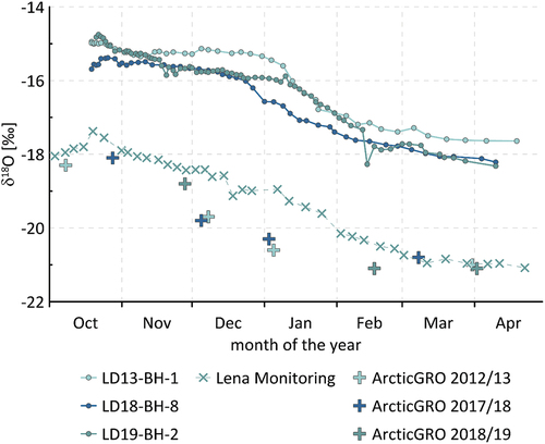
The Lena River is influenced by two different water sources over the course of winter. Rainwater is the dominant water source during summer and fall but is gradually removed from underneath the ice after initial ice cover formation over the first half of winter until the dominant water source is subsurface water (Juhls et al. 2020). This seasonality is also reflected in the isotopic composition of the river ice cores, with the near-constant, relatively heavy isotopic composition in the upper parts of the ice being indicative of rainwater and the progressively lighter isotopic composition indicating the gradual removal of rainwater until isotopically light subsurface water has replaced rainwater as the dominant water source by the end of winter.

Though the seasonal variation of isotope values in river ice from year to year is similar, the reconstructed timing of the decrease from heavy early winter values (e.g., around −15 per mill) to lighter late winter values (around −18 per mill) varies from year to year, starting in late December in 2017–2018 but a few weeks later in 2012–2013 and 2018–2019 (Figure 12), which indicates that the timing of seasonal changes varies significantly between years.

Generally, the calculated dates of changes in isotopic composition in the ice correspond with the observed seasonality of Lena water biogeochemistry and comparing modeled timescales to Lena River water samples revealed that changes in river water sources are transferred into the ice almost immediately. Thus, the Stefan equation has been successfully used to estimate dates for events affecting the isotopic composition of the ice, such as changing water sources.

Conclusions

In a warming Arctic, permafrost landscapes change dramatically and with them the hydrology; that is, the ubiquitous water bodies also change in terms of ice cover dynamics. In particular, duration and timing of ice cover formation play a major role in atmosphere–hydrosphere interactions due to their strong feedbacks to the global climate. By studying the hydrochemistry of Arctic winter ice covers archived in their vertical stable isotope signatures, we explore current control mechanisms of ice cover formation, which is crucial to reducing uncertainties when targeting future changes.

In this study, we present hydrochemical data in a yet unreached 2-cm resolution across all types of water bodies within the Lena River Delta, one of the largest Arctic river deltas and, as such, a key area for understanding hydrological changes in a warming world. We improve on existing studies by sampling across two main (closed- and open-system freezing) types and by using model approaches to correlate field observations and meteorological data.

Based on the ice core data, water body depth was found to act as the main morphometric control of ice cover formation across different hydrological systems. Shallow, medium, and deep water bodies revealed individual characteristics of freezing. In addition, seasonal ice covers reflected local water sources; for example, precipitation for shallow lakes, ground ice melt for Pleistocene lakes, and a shift from rain- to subsurface water sources for the river ice.

When using the Stefan model of ice growth, the alpha values for lakes given by Michel (1971) generally hold, giving ice thickness within +2 cm of observed thicknesses. For river ice, however, the suggested $\mathit{\alpha }$ values lead to an underestimation of ice thicknesses. Instead, alpha values for lake ice are more appropriate. Michel’s (1971) values need to be adapted to a wider range of study areas/conditions; for example, to include rivers that are heavily influenced by snow. The Ashton ice growth model produced ice thicknesses very close to measured values, across both lakes of different depths and the river. However, the model relies on additional in situ observational data, such as snow depth time series, and additional information (exact coring location etc.) to obtain more realistic values. In summary, when assumptions on changing snow depth during the ice growth period are possible or observations of changing snow depth available, the Ashton model provides a better basis for predicting ice growth rates over the winter.

For river ice, the model results reveal that known shifts in river water sources transfer into the ice almost simultaneously. This means that, where continuous water sampling is difficult, ice cores can be used to investigate hydrological changes in water bodies over the course of the winter. Changes in isotopic composition in the ice not only correspond with the observed seasonality of Lena water biogeochemistry but the water isotopic signal is transferred into the ice almost without temporal offset, which means that ice cores can be used to draw conclusions on river water biochemistry below the ice.

The river ice core revealed three phases of different isotopic signature over the course of winter, reflecting the dynamic change in river water sources over that time: The dominant water source is rainwater in the first half of winter, gradually replaced by subsurface water, which remains the only significant water source in the second half of winter. Combining the model results with measured parameters in the ice revealed a link between changing water sources and isotopic fractionation.

The results of this study provide a tool for investigating hydrochemical changes in water bodies that are difficult to sample year-round. They also illustrate the key role of snow cover history on the ice surface over winter when predicting ice growth. The ice growth model provides a useful tool to conclude on seasonal changes in water bodies, which was verified by the close link with the results of the Lena Water Monitoring Program. Studying Arctic winter ice covers provides a crucial basis for future trend analyses, and simple ice growth models may be used to upscale observations of water bodies in remote areas.

Acknowledgments

We thank Mikaela Weiner and Antje Eulenburg for their technical support in the ISOLAB Facility and hydrochemistry laboratories at AWI Potsdam. We also thank all people involved in the organization and logistical support of the Russian–German LENA Expeditions as well as the staff of the Research Station Samoylov Island for their support of our fieldwork in the Lena Delta.

Disclosure statement

No potential conflict of interest was reported by the author(s).

Data availability statement

ArcticGro data are available via https://arcticgreatrivers.org/data/. Lena River Monitoring Program data are available at https://doi.pangaea.de/10.1594/PANGAEA.913197.

Correction Statement

This article has been corrected with minor changes. These changes do not impact the academic content of the article.

References

- Alekseevskii, N. I., D. N. Aibulatov, L. V. Kuksina, and A. A. Chetverova. 2014. The structure of streams in the Lena delta and its influence on streamflow transformation processes. Geography and Natural Resources 35, no. 1: 63–28. doi:10.1134/S1875372814010090.
- Antonova, S., C. Duguay, A. Kääb, B. Heim, M. Langer, S. Westermann, and J. Boike. 2016. Monitoring bedfast ice and ice phenology in lakes of the Lena River Delta using TerraSAR-X backscatter and coherence time series. Remote Sensing 8, no. 11: 903. doi:10.3390/rs8110903.
- Arnason, B. 1969. Equilibrium constant for the fractionation of deuterium between ice and water. The Journal of Physical Chemistry 73, no. 10: 3491–4. doi:10.1021/j100844a062.
- Arp, C. D., B. M. Jones, Z. Lu, and M. S. Whitman. 2012. Shifting balance of thermokarst lake ice regimes across the Arctic Coastal Plain of northern Alaska. Geophysical Research Letters 39: L16503. doi:10.1029/2012GL052518.
- Ashton, G. D. 1989. Thin ice growth. Water Resources Research 25, no. 3: 564–6. doi:10.1029/WR025i003p00564.
- Ashton, G. D. 2011. River and lake ice thickening, thinning, and snow ice formation. Cold Regions Science and Technology 68: 3–19. doi:10.1016/j.coldregions.2011.05.004.
- Bailey, H., A. Hubbard, E. S. Klein, K. R. Mustonen, P. D. Akers, H. Marttila, and J. M. Welker. 2021. Arctic sea-ice loss fuels extreme European snowfall. Nature Geoscience 14, no. 5: 283–8. doi:10.1038/s41561-021-00719-y.
- Bégin, P. N., Y. Tanabe, M. Kumagai, A. I. Culley, M. Paquette, D. Sarrazin, M. Uchida, and W. Vincent. 2021. Extreme warming and regime shift toward amplified variability in a far northern lake. Limnology and Oceanography 66, no. S1: S17–S29. doi:10.1002/lno.11546.
- Bengtsson, L. 2012. Ice formation on lakes and ice growth. In Encyclopedia of lakes and reservoirs. Encyclopedia of earth sciences series, ed. L. Bengtsson, R. W. Herschy, and R. W. Fairbridge. Dordrecht: Springer. doi:10.1007/978-1-4020-4410-6_210.
- Boereboom, T., M. Depoorter, S. Coppens, and J. L. Tison. 2012. Gas properties of winter lake ice in Northern Sweden: Implication for carbon gas release. Biogeosciences 9, no. 2: 827–38. doi:10.5194/bg-9-827-2012.
- Boike, J., C. Georgi, G. Kirilin, S. Muster, K. Abramova, I. Fedorova, A. Chetverova, M. Grigoriev, N. Bornemann, and M. Langer. 2015. Thermal processes of thermokarst lakes in the continuous permafrost zone of northern Siberia – Observations and modeling (Lena River Delta, Siberia). Biogeosciences 12, no. 20: 5941–65. doi:10.5194/bg-12-5941-2015.
- Boike, J., B. Kattenstroth, K. Abramova, N. Bornemann, A. Chetverova, I. Fedorova, K. Fröb, et al. 2013. Baseline characteristics of climate, permafrost and land cover from a new permafrost observatory in the Lena River Delta, Siberia (1998–2011). Biogeosciences 10, no. 3: 2105–28. doi:10.5194/bg-10-2105-2013.
- Boike, J., J. Nitzbon, K. Anders, M. Grigoriev, D. Y. Bolshiyanov, M. Langer, S. Lange, et al. 2019a. A 16-year record (2002–2017) of permafrost, active-layer, and meteorological conditions at the Samoylov Island Arctic permafrost research site, Lena River delta, northern Siberia: An opportunity to validate remote-sensing data and land surface, snow, and permafrost models. Earth System Science Data 11: 261–99. doi:10.5194/essd-11-261-2019.
- Boike, J., J. Nitzbon, K. Anders, M. N. Grigoriev, D. Y. Bolshiyanov, M. Langer, S. Lange, et al. 2018. Meteorologic data at station Samoylov (2002–2018, level 2, version 1). doi:10.1594/PANGAEA.891139.
- Boike, J., J. Nitzbon, K. Anders, M. N. Grigoriev, D. Y. Bolshiyanov, M. Langer, S. Lange, et al. 2019b. Meteorologic data at station Samoylov (2002–2018, level 1, version 201908), link to archive. In: Boike, J. et al. (2019): Measurements in soil and air at Samoylov Station (2002–2018), version 201908. Alfred Wegener Institute - Research Unit Potsdam, PANGAEA, doi:10.1594/PANGAEA.905236. PANGAEA: Alfred Wegener Institute - Research Unit Potsdam. doi:10.1594/PANGAEA.905230.
- Boike, J., C. Wille, and A. Abnizova. 2008. Climatology and summer energy and water balance of polygonal tundra in the Lena River Delta, Siberia. Journal of Geophysical Research: Biogeosciences 113. doi:10.1029/2007JG000540.
- Bonne, J. L., M. Behrens, H. Meyer, S. Kipfstuhl, B. Rabe, L. Schönicke, H. C. Steen-Larsen, and M. Werner. 2019. Resolving the controls of water vapour isotopes in the Atlantic sector. Nature Communications 10, no. 1: 1–10. doi:10.1038/s41467-019-09242-6.
- Budy, P., C. A. Pennock, A. E. Giblin, C. Luecke, D. L. White, and G. W. Kling. 2022. Understanding the effects of climate change via disturbance on pristine Arctic lakes—Multitrophic level response and recovery to a 12-yr, low-level fertilization experiment. Limnology and Oceanography 67, no. S1: S224–S241. doi:10.1002/lno.11893.
- Chetverova, A., T. Skorospekhova, A. Morgenstern, N. Alekseeva, I. Spiridonov, and I. Fedorova. 2017. Hydrological and hydrochemical characteristics of lakes in the Lena River delta (Northeast-Siberia, Russia). Polarforschung 87, no. 2: 111–24. doi:10.2312/polarforschung.87.2.111.
- Clark, I., and P. Fritz. 1997. Environmental isotopes in hydrogeology. Boca Raton: Lewis Publishers.
- Comfort, G., and R. Abdelnour. 2013. Ice thickness prediction: A comparison of various practical approaches. Proceedings 17th CRIPE Workshop on River Ice, 329–42, in Edmonton, Alberta, Canada.
- Craig, H. 1961. Isotopic variations in meteoric waters. Science 133, no. 3465: 1702–3. doi:10.1126/science.133.3465.1702.
- Dansgaard, W. 1964. Stable isotopes in precipitation. Tellus 16, no. 4: 436–68. doi:10.3402/tellusa.v16i4.8993.
- Dibike, Y., T. Prowse, T. Saloranta, and R. Ahmed. 2011. Response of Northern Hemisphere lake-ice cover and lake-water thermal structure patterns to a changing climate. Hydrological Processes 25, no. 19: 2942–53. doi:10.1002/hyp.8068.
- Duguay, C. R., T. D. Prowse, B. R. Bonsal, R. D. Brown, M. P. Lacroix, and P. Ménard. 2006. Recent trends in Canadian lake ice cover. Hydrological Processes 20, no. 4: 781–801. doi:10.1002/hyp.6131.
- Fedorova, I., A. Chetverova, D. Bolshiyanov, A. Makarov, J. Boike, B. Heim, A. Morgenstern, et al. 2015. Lena Delta hydrology and geochemistry: Long-term hydrological data and recent field observations. Biogeosciences 12, no. 2: 345–63. doi:10.5194/bg-12-345-2015.
- Ferrick, M. G., D. J. Calkins, N. M. Perron, J. H. Cragin, and C. Kendall. 2002. Diffusion model validation and interpretation of stable isotopes in river and lake ice. Hydrological Processes 16, no. 4: 851–72. doi:10.1002/hyp.374.
- French, H. M. 2007. Permafrost. In The periglacial environment, ed. H. M. French, 83–115. doi:10.1002/9781118684931.
- Fritz, M., S. Wetterich, H. Meyer, L. Schirrmeister, H. Lantuit, and W. H. Pollard. 2011. Origin and characteristics of massive ground ice on Herschel Island (western Canadian Arctic) as revealed by stable water isotope and hydrochemical signatures. Permafrost and Periglacial Processes 22, no. 1: 26–38. doi:10.1002/ppp.714.
- Fuchs, M., D. Bolshiyanov, M. Grigoriev, A. Morgenstern, L. Pestryakova, L. Tsibizov, and A. Dill. 2021. Russian-German cooperation: Expeditions to Siberia in 2019. In Berichte zur Polar- und Meeresforschung = Reports on polar and marine research, Vol. 749, 272. Bremerhaven: Alfred Wegener Institute for Polar and Marine Research. doi:10.48433/BzPM_0749_2021.
- Gibson, J. J., and T. D. Prowse. 1999. Isotopic characteristics of ice cover in a large northern river basin. Hydrological Processes 13, no. 16: 2537–48. doi:10.1002/(SICI)1099-1085(199911)13:163.3.CO;2-1.
- Gibson, J. J., and T. D. Prowse. 2002. Stable isotopes in river ice: Identifying primary over-winter streamflow signals and their hydrological significance. Hydrological Processes 16, no. 4: 873–90. doi:10.1002/hyp.366.
- Greene, G. M., and S. I. Outcalt. 1985. A simulation model of river ice cover thermodynamics. Cold Regions Science and Technology 10, no. 3: 251–62. doi:10.1016/0165-232X(85)90036-9.
- Griffiths, K., N. Michelutti, M. Sugar, M. S. V. Douglas, and J. P. Smol. 2017. Ice-cover is the principal driver of ecological change in High Arctic lakes and ponds. PLOS ONE 12, no. 3: e0172989. doi:10.1371/journal.pone.0172989.
- Grigoriev, M. N. 1993. Cryomorphogenesis in the Lena Delta, 176. Yakutsk: Permafrost Institute Press. (in Russian).
- Grigoriev, N. F. 1960. The temperature of permafrost in the Lena delta basin–deposit conditions and properties of the permafrost in Yakutia. Yakutsk 2: 97–101. (in Russian).
- Heim, B., S. Lisovski, M. Wieczorek, A. Morgenstern, B. Juhls, I. Shevtsova, S. Kruse, J. Boike, I. Fedorova, and U. Herzschuh. 2022. Spring snow cover duration and tundra greenness in the Lena Delta, Siberia: Two decades of MODIS satellite time series (2001–2021). Environmental Research Letters 17, no. 8: 085005. doi:10.1088/1748-9326/ac8066.
- Höfle, S. T. 2015. Organic matter composition and dynamic in polygonal tundra soils. Dissertation, Universität zu Köln.
- Holmes, R. M., J. W. McClelland, S. E. Tank, R. G. M. Spencer, and A. I. Shiklomanov. 2021. Arctic Great Rivers Observatory. Water Quality Dataset, Version 2022-09-10. https://www.arcticgreatrivers.org/data.
- Jeffries, M. O., K. Morris, and C. R. Duguay. 2012. Floating ice: Lake ice and river ice. Satellite image atlas of glaciers of the world – state of the earth’s cryosphere at the beginning of the 21st century: Glaciers, global snow cover, floating ice, and permafrost and periglacial environments. Reston, Virginia: U.S. Geological Survey.
- Juhls, B., S. Antonova, M. Angelopoulos, N. Bobrov, M. Grigoriev, M. Langer, G. Maksimov, F. Miesner, and P. P. Overduin. 2021. Serpentine (floating) ice channels and their interaction with riverbed permafrost in the Lena River Delta, Russia. Frontiers in Earth Science 9, no. 689941. doi:10.3389/feart.2021.689941.
- Juhls, B., C. A. Stedmon, A. Morgenstern, H. Meyer, J. Hölemann, B. Heim, V. Povazhnyi, and P. P. Overduin. 2020. Identifying drivers of seasonality in Lena River biogeochemistry and dissolved organic matter fluxes. Frontiers in Environmental Science 8, no. 53. doi:10.3389/fenvs.2020.00053.
- Kruse, S., D. Bolshiyanov, M. N. Grigoriev, A. Morgenstern, L. Pestryakova, L. Tsibizov, and A. Udke. 2019. Russian-German cooperation: expeditions to Siberia in 2018. In Berichte zur Polar- und Meeresforschung = Reports on polar and marine research, Vol. 734, 257. Bremerhaven: Alfred Wegener Institute for Polar and Marine Research. doi:10.2312/BzPM_0734_2019.
- Lacelle, D. 2011. On the δ18O, δD and D-excess relations in meteoric precipitation and during equilibrium freezing: Theoretical approach and field examples. Permafrost and Periglacial Processes 22: 13–25. doi:10.1002/ppp.712.
- Langer, M., S. Westermann, S. Muster, K. Piel, and J. Boike. 2011. The surface energy balance of a polygonal tundra site in northern Siberia – Part 2: Winter. The Cryosphere 5: 509–524. doi:10.5194/tc-5-509-2011.
- Langer, M., S. Westermann, A. K. Walter, K. Wischnewski, and J. Boike. 2015. Frozen ponds: Production and storage of methane during the Arctic winter in a lowland tundra landscape in northern Siberia, Lena River delta. Biogeosciences 12, no. 4: 977–90. doi:10.5194/bg-12-977-2015.
- Li, X., D. Long, Q. Huang, and F. Zhao. 2022. The state and fate of lake ice thickness in the Northern Hemisphere. Science Bulletin 67, no. 5: 537–46. doi:10.1016/j.scib.2021.10.015.
- Lotsari, E., L. Lind, and M. Kämäri. 2019. Impacts of hydro-climatically varying years on ice growth and decay in a subarctic river. Water 11, no. 10: 2058. doi:10.3390/w11102058.
- Ma, X., and Y. Fukushima. 2002. A numerical model of the river freezing process and its application to the Lena River. Hydrological Processes 16, no. 11: 2131–40. doi:10.1002/hyp.1146.
- Magritsky, D. V., D. N. Aibulatov, and A. V. Gorelkin. 2018. Regularities in the space and time flow variations in the near-mouth reach and delta of the Lena River. Water Resources 45, no. 1: 12–26. doi:10.1134/S009780781801013X.
- Ma, X., T. Yasunari, and Y. Fukushima. 2002. Modeling of river ice breakup date and thickness in the Lena River. In Ice in the Environment, Proceedings of the 16th IAHR International Symposium on Ice, 15, December 2–6, Dunedin, New Zealand: International Association of Hydraulic Engineering and Research.
- Meyer, H., L. Schönicke, U. Wand, H. W. Hubberten, and H. Friedrichsen. 2000. Isotope studies of hydrogen and oxygen in ground ice - experiences with the equilibration technique. Isotopes in Environmental and Health Studies 36, no. 2: 133–49. doi:10.1080/10256010008032939.
- Michel, B. 1971. Winter regime of rivers and lakes. Hanover, New Hampshire, U.S. Army cold regions research and engineering laboratory (CRREL). CREEL Monograph 111-B1a: 130.
- Morgenstern, A., G. Grosse, F. Günther, I. Fedorova, and L. Schirrmeister. 2011. Spatial analyses of thermokarst lakes and basins in Yedoma landscapes of the Lena Delta. The Cryosphere 5: 849–67. doi:10.5194/tc-5-849-2011.
- Morgenstern, A., G. Grosse, L. Schirrmeister. 2008. Genetic, morphological, and statistical characterization of lakes in the permafrost-dominated Lena Delta. In Permafrost: Proceedings of the 9th International Conference on Permafrost, 29 June - 3 July 2008, Fairbanks, Alaska, ed. D. L. Kane and K. M. Hinkel, 1239–1244. Institute of Northern Engineering, University of Alaska Fairbanks.
- Morgenstern, A., C. Röhr, G. Grosse, and M. N. Grigoriev. 2011. The Lena River Delta - inventory of lakes and geomorphological terraces [dataset]. PANGAEA: Alfred Wegener Institute - Research Unit Potsdam. doi:10.1594/PANGAEA.758728.
- Morgenstern, A., M. Ulrich, F. Günther, S. Roessler, I. V. Fedorova, N. A. Rudaya, S. Wetterich, J. Boike, and L. Schirrmeister. 2013. Evolution of thermokarst in East Siberian ice rich permafrost: A case study. Geomorphology 201: 363–79. doi:10.1016/j.geomorph.2013.07.011.
- Murfitt, J. C., L. C. Brown, and S. E. Howell. 2018. Estimating lake ice thickness in Central Ontario. PLOS ONE 13, no. 12: e0208519. doi:10.1371/journal.pone.0208519.
- Muskett, R. 2012. Remote sensing, model-derived and ground measurements of snow water equivalent and snow density in Alaska. International Journal of Geosciences 3: 1127–36. doi:10.4236/ijg.2012.35114.
- Muster, S., M. Langer, B. Heim, S. Westermann, and J. Boike. 2012. Subpixel heterogeneity of ice-wedge polygonal tundra: A multi-scale analysis of land cover and evapotranspiration in the Lena River Delta, Siberia. Tellus B: Chemical and Physical Meteorology 64, no. 1: 17301. doi:10.3402/tellusb.v64i0.17301.
- Muster, S., W. J. Riley, K. Roth, M. Langer, F. Cresto Aleina, C. D. Koven, S. Lange et al, 2019. Size distributions of arctic waterbodies reveal consistent relations in their statistical moments in space and time. Frontiers in Earth Science 7. doi:10.3389/feart.2019.00005.
- Muster, S., K. Roth, M. Langer, S. Lange, F. Cresto Aleina, A. Bartsch, A. Morgenstern, et al. 2017. PeRL: A circum-Arctic permafrost region pond and lake database. Earth System Science Data 9: 317–48. doi:10.5194/essd-9-317-2017.
- Overduin, P., F. Blender, D. Y. Bolshiyanov, M. N. Grigoriev, A. Morgenstern, and H. Meyer. 2017. Russian-German cooperation: Expeditions to Siberia in 2016. Berichte zur Polar- und Meeresforschung = Reports on polar and marine research, Vol. 709, 295. Bremerhaven: Alfred Wegener Institute for Polar and Marine Research. doi:10.2312/BzPM_0709_2017.
- Prowse, T., K. Alfredsen, S. Beltaos, B. R. Bonsal, W. B. Bowden, C. R. Duguay, A. Korhola, et al. 2011. Effects of changes in Arctic lake and river ice. Ambio 40: 63–74. doi:10.1007/s13280-011-0217-6.
- Rantanen, M., A. Y. Karpechko, A. Lipponen, K. Nordling, O. Hyvärinen, K. Ruosteenoja, T. Vihma, and A. Laaksonen. 2022. The Arctic has warmed nearly four times faster than the globe since 1979. Communications Earth & Environment 3, no. 168: 1–10. doi:10.1038/s43247-022-00498-3.
- Schirrmeister, L., D. Froese, V. Tumskoy, G. Grosse, and S. Wetterich. 2013. Yedoma: Late Pleistocene ice-rich syngenetic permafrost of Beringia. The Encyclopedia of Quaternary Science 3: 542–52. doi:10.1016/b978-0-444-53643-3.00106-0.
- Schneider, J., G. Grosse, and D. Wagner. 2009. Land cover classification of tundra environments in the Arctic Lena Delta based on Landsat 7 ETM+ data and its application for upscaling of methane emissions. Remote Sensing of Environment 113, no. 2: 380–91. doi:10.1016/j.rse.2008.10.013.
- Schwamborn, G., V. Rachold, and M. N. Grigoriev. 2002. Late Quaternary sedimentation history of the Lena Delta. Quaternary International 89, no. 1: 119–34. doi:10.1016/S1040-6182(01)00084-2.
- Schwamborn, G., L. Schirrmeister, A. Mohammadi, H. Meyer, A. Kartoziia, F. Maggioni, and J. Strauss. 2023. Fluvial and permafrost history of the lower Lena River, north-eastern Siberia, over late Quaternary time. Sedimentology 70: 235–58. doi:10.1111/sed.13037.
- Sentinel Hub. 2023. https://www.sentinel-hub.com/ (accessed October 15, 2022).
- Shafique, U., J. Anwar, M. A. Munawar, W. U. Zaman, R. Rehman, A. Dar, M. Saleem, et al. 2016. Chemistry of ice: Migration of ions and gases by directional freezing of water. Arabian Journal of Chemistry 9: 47–53. doi:10.1016/j.arabjc.2011.02.019.
- Sharma, S., K. Blagrave, J. J. Magnuson, C. M. O’Reilly, S. Oliver, R. D. Batt, M. R. Magee, et al. 2019. Widespread loss of lake ice around the Northern Hemisphere in a warming world. Nature Climate Change 9: 227–31. doi:10.1038/s41558-018-0393-5.
- Shiklomanov, A. I., and R. B. Lammers. 2014. River ice responses to a warming Arctic—recent evidence from Russian rivers. Environmental Research Letters 9, no. 3: 035008. doi:10.1088/1748-9326/9/3/035008.
- Skorospekhova, T., B. Heim, A. Chetverova, I. Fedorova, N. Alekseeva, O. Bobrova, Y. Dvornikov, A. Eulenburg, S. Roessler, and A. Morgenstern. 2018. Coloured dissolved organic matter variability in tundra lakes of the Central Lena River Delta (N-Siberia). Polarforschung 87, no. 2: 125–34. doi:10.2312/polarforschung.87.2.125.
- Spangenberg, I., P. P. Overduin, E. Damm, I. Bussmann, H. Meyer, S. Liebner, M. Angelopoulos, B. Biskaborn, M. Grigoriev, and G. Grosse. 2020. Methane pathways in winter ice of thermokarst lakes, lagoons and coastal waters in North Siberia. The Cryosphere Discussions 1–28. doi:10.5194/tc-2019-304.
- Spors, S. 2018. Stable water isotope characteristics of recent precipitation from Tiksi and Samoylov island – calibration of a geoscientific proxy for Northern Siberia. Bachelor Thesis, University of Potsdam.
- Stefan, J. 1891. Über die Theorie der Eisbildung, insbesondere über Eisbildung im Polarmeere. Annalen der Physik und Chemie 42, no. 2: 269–86. doi:10.1002/andp.18912780206.
- Stolpmann, L., G. Mollenhauer, A. Morgenstern, J. S. Hammes, J. Boike, P. P. Overduin, and G. Grosse. 2022. Origin and pathways of dissolved organic carbon in a small catchment in the Lena River Delta. Frontiers in Earth Science 9. doi:10.3389/feart.2021.759085.
- Sturm, M., and G. E. Liston. 2003. The snow cover on lakes of the Arctic Coastal Plain of Alaska, U.S.A. Journal of Glaciology 49, no. 166: 370–80. doi:10.3189/172756503781830539.
- Surdu, C. M., C. R. Duguay, L. C. Brown, and D. Fernández Prieto. 2014. Response of ice cover on shallow lakes of the North Slope of Alaska to contemporary climate conditions (1950–2011): Radar remote-sensing and numerical modeling data analysis. The Cryosphere 8, no. 1: 167–80. doi:10.5194/tc-8-167-2014.
- Surma, J., S. Assonov, M. J. Bolourchi, and M. Staubwasser. 2015. Triple oxygen isotope signatures in evaporated water bodies from the Sistan Oasis, Iran. Geophysical Research Letters 42, no. 20: 8456–62. doi:10.1002/2015GL066475.
- Suzuoki, T., and T. Kimura. 1973. D/H and 18O/16O fractionation in ice-water system. Journal of the Mass Spectrometry Society of Japan 21, no. 3: 229–33. doi:10.5702/MASSSPEC1953.21.229.
- Taulu, J. 2022. An assessment of seasonal source water contributions to streamflow in the Athabasca River Basin, utilizing a novel approach to obtain a record of winter streamflow from river ice stratigraphy, M.Sc. thesis, Department of Geography, University of Victoria.
- U.S. Army Corps of Engineers. 2002. Ice Engineering, EM 1110-2-1612. Washington, DC: Department U.S. Army Corps of Engineers. http://www.usace.army.mil/publications/engmanuals/em1110-2-1612/toc.htm.
- Walter Anthony, K. M., D. A. Vas, L. Brosius, F. S. Chapin, S. A. Zimov, and Q. Zhuang. 2010. Estimating methane emissions from northern lakes using ice-bubble surveys. Limnology and Oceanography - Methods 8: 592–609. doi:10.4319/lom.2010.8.0592.
- Wetterich, S., S. Kuzmina, A. A. Andreev, F. Kienast, H. Meyer, L. Schirrmeister, T. Kuznetsova, and M. Sierralta. 2008. Palaeoenvironmental dynamics inferred from late Quaternary permafrost deposits on Kurungnakh Island, Lena Delta, northeast Siberia, Russia. Quaternary Science Reviews 27, no. 15–16: 1523–40. doi:10.1016/j.quascirev.2008.04.007.
- Wik, M., P. M. Crill, D. Bastviken, Å. Danielsson, and E. Norbäck. 2011. Bubbles trapped in Arctic lake ice: Potential implications for methane emissions. Journal of Geophysical Research 116, no. G03044. doi:10.1029/2011JG001761.
- Yen, Y.-C. 1981. Review of thermal properties of snow, ice and sea ice. CRREL Report 81-10, Cold Regions Research and Engineering Laboratory, 27. Hanover, NH: U.S. Army Corps of Engineers.
- Yoshikawa, Y., Y. Watanabe, and A. Itoh. 2014. A simple equation for ice sheet thickness and ice formation/breakup prediction. Journal of JSCE 2, no. 1: 203–13. doi:10.2208/journalofjsce.2.1_203.
- Zhang, T., and M. O. Jeffries. 2000. Modeling interdecadal variations of lake-ice thickness and sensitivity to climatic change in northernmost Alaska. Annals of Glaciology 31: 339–47. doi:10.3189/172756400781819905.
- Zhang, F., Z. Li, and K. E. Lindenschmidt. 2019. Potential of RADARSAT-2 to improve ice thickness calculations in remote, poorly accessible areas: A case study on the Slave River, Canada. Canadian Journal of Remote Sensing 45, no. 2: 234–45. doi:10.1080/07038992.2019.1567304.