Integrated differentiation of multiple trichloroethylene and tetrachloroethylene groundwater impacts using spatial concentration, biodegradation indices, chemical fingerprinting and carbon/chlorine isotope patterns

Abstract

Conventional testing methods provide sufficient information to evaluate human or ecological risk. However, contaminant concentrations patterns alone provide only limited resolution of important liability issues, such as when and where did contaminant releases originate. Over the past few decades, scientists explored the isotope applications to better identify, delineate, and manage contaminants in the environment. Advanced chemical fingerprinting and isotope technologies revealed important linkages between isotope ratios and contaminant origins (e.g., chemical feedstock and manufacturing process). Studies of environmental weathering distinguished abiotic and biotic changes in the chemical composition and isotope patterns. The combined application of chemical and isotopic fingerprints offers powerful complementary lines of evidence for delineating contaminants, assessing risk, and identifying historical sources. This manuscript provides an integrated forensic approach that systematically links conventional environmental investigation data with specialized chemical fingerprinting and carbon/chlorine isotope methods for identifying the sources of groundwater impacts especially when multiple potential point and non-point sources exist. This paper focusses on chlorinated solvents. Specifically, it features the synoptic use of chemical concentration patterns and compound-specific isotope analysis (CSIA) as effective tools for confirming organic contaminant sources, characterizing environmental weathering, and answering a growing list of site-specific questions. Unlike conventional isotope methods, which can be both time-consuming and expensive, this paper presents an optimized analytical method for chlorine CSIA using gas chromatography-quadrupole mass spectrometry (GC-qMS). Chlorine isotopic composition for multiple analytes (e.g., tetrachloroethylene [PCE], trichloroethylene [TCE], dichloroethylene [DCE], and vinyl chloride [VC]) can be determined in one acquisition thus reducing analysis time and cost. Precise CSIA isotope values were achieved for chloroethylene concentrations between approximately 5 micrograms per liter (ug/l) and 100 ug/l for carbon and between approximately 30 ug/l to 1,000 ug/l for chlorine. The gradual improvement in CSIA methods better addresses the wide concentration range encountered in typical samples collected from groundwater aquifers with significant chlorinated solvent impacts. A case study is presented featuring a tiered forensic investigation using spatial chemistry and isotope patterns to evaluate commingled plumes of PCE and TCE.

Keywords:

• Tetrachloroethylene
• trichloroethylene
• organohalide respiration
• dechlorination
• compound-specific isotope analysis
• quadrupole mass spectrometry

Introduction

Chlorinated solvents PCE and TCE found widespread use over the past century in degreasing and dry-cleaning operations (Doherty, 2000). Chlorinated solvents are volatile, immiscible in water, denser than water, and exhibit varying solubilities (Pankow and Cherry, 1996; National Library of Medicine, 2021). As such, when chlorinated solvents are released into the environment through accidental spills and leaks, they can readily migrate through subsurface media and contaminate groundwater. PCE and TCE, as well as degradation products 1,1-dichloroethene (DCE11) and VC are classified as either carcinogenic or as probable carcinogens and are regulated at very low concentrations, particularly in groundwater and drinking water (ATSDR 2019a, 1996, 2019b, 2019c, 2006). Identifying the source of chlorinated solvent plumes and assessing the fate of chlorinated volatile organic compounds (CVOCs) in the environment are common issues faced by environmental scientists and regulators especially when vapor intrusion is a concern or groundwater serves as a potential source of potable water.

Environmental site assessments typically determine the concentrations of CVOCs, such as PCE and its degradation products TCE, DCE, and VC using standard sampling and analytical methods. These investigations focus on the nature and extent of contaminants that exceed applicable regulatory limits and estimate the degree of risk posed to human and ecological receptors. Environmental forensic investigations focus on contaminant origins from the perspective of liability (i.e., who is responsible for the contaminant release) and cost allocation using additional lines of evidence based on routine environmental data, often augmented by data generated using non-routine analytical techniques.

Identifying the source(s) of PCE and TCE released into the environment is complex. Chlorinated solvents have a variety of candidate historical sources; thus, multiple point sources often exist at sites impacted by chlorinated solvents. These contaminants often migrate away from points of release and environmentally degrade over time and space, further complicating source identification. The ability to distinguish multiple point sources and assess impacts due to weathering are important factors for determining liability at sites impacted by chlorinated solvents and greatly assisted by multiple lines of evidence (MLE) including CSIA data.

The isotopic composition of many contaminants is initially established at the time these chemicals are manufactured. For example, the carbon and chlorine isotope content are determined by the isotopic content of the starting compounds (e.g., ethane from petroleum and chlorine from brine) used to manufacture the dry-cleaning solvent (e.g., PCE), with possible changes introduced by the manufacturing process, such as exposure to elevated temperature, high/low pressure and catalytic surfaces (Jendrzejewski et al., 2001). The manufacturing process creates abiotic conditions that tend to “fractionate” lighter isotopes from heavier isotopes. This fractionation is a kinetic isotope reaction, so it will not reverse itself spontaneously and it progresses in one primary direction. Changes in the origin of starting compounds for manufacturing processes can result in chemical products (e.g., fuels, petrochemicals, solvents, dry cleaning fluids, and degreasing solvents) having different isotopic signatures (Beneteau et al., 1999; Shouakar-Stash et al., 2003). Carbon and chlorine isotopic composition can vary between different manufacturers and batches of the same product (van Warmerdam et al., 1995; Beneteau et al., 1999; Jendrzejewski et al., 2001; Shouakar-Stash et al., 2003).

Once released into the environment, isotopic signatures can change due to environmental weathering primarily caused by evaporation, dissolution, and biodegradation. For example, waste dry cleaning solvent (e.g., PCE) spilled onto a parking lot surface will evaporate, while a subsurface pipe leak of PCE into subsurface soil may biodegrade under anaerobic conditions. In either case, isotopic fractionation causes the solvent residue to become isotopically heavier than the starting material (Brand and Coplen, 2012). This enrichment reflects the slightly higher propensity of compounds with lighter isotopes to evaporate or metabolize, leaving the heavier isotopes in the degraded residue. Organohalide respiration causes significant isotopic fractionation (> 2 ‰) for both carbon and chlorine and provides in situ evidence of biodegradation (Lollar et al., 1999; Slater et al., 2001; Numata et al., 2002; Hunkeler et al., 2008; Wiegert et al., 2012). The sequential biodegradation of PCE, TCE, DCE, and VC can be site-specific, because it depends on the presence of bacterial species capable of specializing in the metabolism of specific substrates (i.e., contaminants) living in specific hydrogeological conditions (Leys et al., 2013; Heckel et al., 2018; Lihl et al., 2019). Despite the specialized nature of organohalide respiration, it’s isotopic signature is well documented and frequently observed (Meckenstock et al., 2004; Hunkeler et al., 2008; Wiegert et al., 2012). Recognizing biodegradation is of particular importance for sites employing monitored natural attenuation (MNA) as part of a remedy strategy, because MNA guidelines often mandate the collection of sufficient chemical monitoring data to demonstrate contaminant transformations (not dilution) inherent to MNA over time. The need to demonstrate biodegradation can require the installation of monitoring wells, re-sampling, and extensive documentation. By contrast, isotopic changes (spatial and temporal) efficiently provide scientific proof that the mass of the contaminant and byproducts are changing due to biodegradation during a limited number of sampling rounds.

Though CSIA provides information pertinent to contaminant origin and weathering, factors such as cost and lengthy turnaround times have limited the routine use of CSIA in environmental investigations. In part, costs arise from the expense of conventional isotope instrumentation and time-consuming offline sample preparation sometimes required by isotope laboratories.

The practical limitations of isotope testing vary by technology. Conventional isotope analysis by isotope ratio mass spectrometry (IRMS) employs Faraday cup detectors that measure ion currents simultaneously, resulting in very precise isotope ratio measurements, typically < 0.5 ‰. However, IRMS is constrained by specific Faraday cup configurations and a narrow range of concentrations for which precise stable isotope measurements can be achieved (Meier-Augenstein, 1999; Elsner et al., 2012; Jochmann and Schmidt, 2013). Traditional Cl isotope analysis by dual inlet (DI) IRMS requires time-consuming offline preparation methods to quantitatively convert Cl into chlorinated gases such as CH₃Cl for analysis (Holt et al., 1997). DI-IRMS techniques are unable to measure more than one CVOC present in a sample without the use of offline separation methods.

GC-IRMS techniques are available for chlorine isotope analysis that allow for online separation. High temperature conversion of chlorinated contaminants, in the presence of H₂, generates hydrochloric acid. Chlorine isotope ratios are determined by a mass spectrometer capable of measuring the abundances of ions with mass-to-charge ratio (m/z) 36 for H³⁵Cl relative to m/z 38 for H³⁷Cl (Renpenning et al., 2015). Academic and instrument manufacturers developed analytical techniques in which chlorinated solvents are analyzed directly, without first converting to a common gas. For example, the chlorine isotopic composition of vinyl chloride has been measured by directly monitoring molecular ions m/z 64 (C₂H³⁷Cl) and m/z 62 (C₂H³5Cl) and comparing chlorine isotope ratios relative to reference gas pulses of vinyl chloride. This technique generates precise chlorine isotope measurements but is limited in by an inability to measure more than one target analyte per sample (Shouakar-Stash et al., 2006). Alternative online techniques determine ³⁷Cl/³⁵Cl ratios of volatile and semivolatile contaminants using a gas chromatograph coupled to multiple-collector inductively coupled plasma mass spectrometer (GC-MC-ICPMS), which offer significant promise for isotope studies once robust sample preparation techniques for water and soil are developed (Horst et al., 2017; Renpenning et al., 2018).

Concurrently, researchers developed methods for chlorine CSIA analysis by GC-qMS operated in selected ion monitoring (SIM) mode (Sakaguchi-Soder et al., 2007; Aeppli et al., 2010). Quadrupole mass spectrometers achieve adequate sensitivity over wider calibration ranges than IRMS detectors; thus, these instruments are well-suited to measure the range of chlorinated solvent concentrations found in environmental field samples. However, qMS lacks the degree of precision necessary for measuring stable isotopes of elements such as carbon and hydrogen due to the low natural abundance of the heavy (or rare) isotope for these elements (1.11% and 0.015% respectively). Chlorine is an exception because the natural abundance of the heavy (or rare) isotope of chlorine (³⁷Cl) is high enough (24.11%) such that precise chlorine isotope ratios can be obtained using a qMS operated in SIM mode (Bernstein et al., 2011; Jin et al., 2011). However, published methods for determining the chlorine isotopic composition of chlorinated solvents by GC-qMS have not been optimized for routine field applications (e.g., wide ranging concentrations of multiple target analyte detections per acquisition for large sample deliveries with short turnaround times).

Technological innovations incrementally improve the capacity of MLE investigations to characterize contaminant sources and migration pathways in the environment. This work features recent optimization of published GC-qMS methods for chlorine isotope analysis that can be applied to multiple analytes (PCE, TCE, DCE isomers, and VC) in one acquisition. Precise isotope measurements were determined for chlorinated contaminant concentrations above approximately 30 ug/l, depending on the analyte. This method can be adapted into a commercial lab setting and integrated into MLE investigations that include conventional field and VOC testing methods as well as specialized GC/IRMS carbon isotope testing. The utility of this integrated approach is illustrated by a case study involving the determination of CVOC origins at a site with multiple potential sources and an uncertain hydrogeologic setting.

Materials and methods

Five lines of evidence (LOE) provide a robust framework for CVOC source identification. The LOEs include parent contaminant concentrations, non-target analytes (NTCs), chemical biodegradation indices (BDIs), and carbon/chlorine isotope ratios by CSIA methods. The spatial dimension of these LOEs help isolate contaminant source signatures (i.e., chemical fingerprints) and track them through the study area. The parent contaminant declines gradually and systematically as it migrates away from the source area and mixes with increasingly larger proportions of ambient media. Frequently this decline reflects microbial degradation, the magnitude of which depends heavily on the oxygen content, electron receptors, and other constituents of groundwater and soil through which the contaminants migrate. Biotic (anaerobic and aerobic) and abiotic (chemical reduction) degradation processes create isotopically heavier distributions of carbon and chlorine in the unreacted parent compounds and degradation byproducts over time (Abe et al., 2009; Kuder et al., 2013). By contrast, physical processes, such as dilution, do not significantly alter the carbon and chlorine isotope ratios in the unreacted parent compounds (Meckenstock et al., 2004). In addition, releases of spent solvent can contain co-occurring constituents (e.g., fats, oils, greases, dyes, pigments, plasticizers, and others) that can help distinguish fugitive solvent waste generated by distinct historical activities.

These lines of evidence help differentiate CVOC sources and impacts when multiple candidate sources exist, especially when contextualized spatially. For example, groundwater concentrations that increase in a distant part of the plume signify the presence of additional sources. Similarly, the detection of fresh solvent in a distant part of a weathered solvent plume signifies the presence of additional contaminant sources. Finally, the appearance of co-occurring constituents, like petroleum hydrocarbons or dyes, in a localized area of the groundwater plume can indicate changes in the groundwater direction or localized impacts from proximal pipes or small-scale chronic releases over time. Collectively, the spatial distribution of groundwater constituents is well suited for the study of groundwater contaminant sources, contaminant delineation, and prevailing groundwater direction.

Study area geology and hydrology

The coastal study area (Figure 1) was topographically flat consisting of heterogeneous fill extending to approximately 8 to 20 feet (ft) (2.4 to 6.1 meters [m]) below ground surface (bgs) emplaced over organic soils attributed to historical meadow matt or peat (approximately 1-2 ft [0.30 − 0.61 m] thick) and underlain by a continuous water bearing unit composed of two sand deposits. The upper sand unit consisted of Quaternary Terrace sand that increased in thickness from about 1 ft (0.30 m) in the northwest study area to approximately 16 ft (4.9 m) along the tributary flowing along the southeast boundary of the study area. The lower Farrington Sand varied in thickness from approximately 6 to 8 ft (1.8 to 2.4 m) throughout the study area. Saprolite bedrock confined the shallow aquifer at depths ranging from approximately 20 ft (6.1 m) in the northwest to 30 ft (9.1 m) in the southeast study area. Groundwater elevation varied seasonally between 5 and 8 ft (1.5 and 2.4 m) bgs with minor tidal effects within approximately 100 ft (30 m) of a northeasterly flowing tributary along its southern boundary.

Figure 1. Site features: (a) A metal fabricator (Source 1), dry cleaner (Source 2), and/or auto service station (Source 3) allegedly released CVOCs that contaminated groundwater. (b) The piezometric surface based upon twenty-three groundwater monitoring wells (a-w) demonstrated southeasterly groundwater flow (average piezometric contours and inferred groundwater direction arrows in grey) that shifted more southerly or easterly depending on the sampling location/date and hydrological model assumptions. The forensic objective was to determine if CVOCs from Sources 1 and 2 impacted Downgradient Zones A, B, and C using chemical and isotopic fingerprinting.

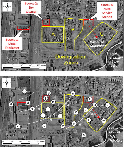
Chlorinated solvents were historically used at a metal fabricator (Source 1), a dry cleaner (Source 2) and auto service station (Source 3). Exact solvent purchase and disposal records were largely unavailable. A former drainage channel was thought to flow from Source 3 to the tributary, although modern development made this difficult to confirm. Sources 1, 2, and 3 were initially associated with chloroethylene detections that exceeded applicable regulatory standards (Table 1) in three proximal Downgradient Zones (Figure 1a A, B, and C). Twenty-three groundwater monitoring wells (Figure 1b, MW-a to MW-w or simply a to w) were installed through the fill and sand layers to the bedrock (2” [5 cm] diameter, 10 ft [3.1 m] screen interval, and filter pack) in accordance with industry standard practice (Aller et al., 1991; ASTM 2016). Seasonal groundwater elevation monitoring demonstrated southeasterly flow to the tidal tributary (Figure 1b). However, the piezometric surface varied southerly or easterly over time and was unable to definitively allocate responsibility for remedial activities in each Downgradient Zone. This forensic investigation generated additional lines of evidence to help reconcile the origin of CVOCs in each Downgradient Zone with an emphasis on determining the degree to which historical releases from Sources 1 or 2 created impacts in Downgradient Zone C.

Table 1. Selected physical and chemical properties of chloroethylene target analytes. Pure PCE and TCE products possess higher molecular weights capable of sinking through groundwater with lower propensities to dissolve in water or volatilize in vapor compared to DCE and VC byproducts. Analyte reference information, such as the chemical abstract number (CAS), is provided to avoid potential confusion with similar compounds. Units are grams per cubic centimeter (g/cm³), degrees Celsius (°C), micromole per liter (um/l), and atmosphere cubic meters per mole (atm m³/mol).

Chloroethylene Analyte	Abbrev	CAS	Molecular Weight	Formula	Density @20 °C g/cm^3	Boiling Point °C	Melting Point °C	Water Solubility @ 25 °C um/l	Henry's Law Constant atm m^3 mol^-1	State GW Limits um/l
Tetrachloroethylene	PCE	127-18-4	165.87	C2Cl4	1.62	121	−22.2	1240	0.02	0.0024
Trichloroethylene	TCE	79-01-6	131.39	C2HCl3	1.46	87.2	−84.7	9740	0.01	0.0076
cis-1,2-Dichloroethylene	DCEc12	156-59-2	96.95	C2H2Cl2	1.28	60.0	−80.0	66100	0.01	0.72
trans-1,2-Dichloroethylene	DCEt12	156-60-5	96.95	C2H2Cl2	1.26	47.6	−49.8	46600	0.01	1.0
1,1-Dichloroethylene	DCE11	75-35-4	96.94	C2H2Cl2	1.21	31.6	−123	25000	0.03	0.010
Vinyl chloride	VC	75-01-4	62.50	C2H3Cl	0.911	−13.9	−154	141000	0.03	0.0013
Source:	Hazardous Substance Data Bank (https://pubchem.ncbi.nlm.nih.gov/source/hsdb)

Collection of samples

Field sampling procedures exert significant influence on the quality of VOC groundwater assessments. The study area grew as periodic monitoring data was collected over several years. Split samples for forensic characterization were collected in Spring (Sampling Event 1) and Summer (Sampling Event 2). The field sampling team collected groundwater using low flow sampling equipment to fill a minimum of three pre-cleaned 40 mL glass VOC vials fortified with 2-4 drops of 1:1 hydrochloric acid (HCl) that reduced the sample pH below 2 to minimize biodegradation of VOCs before analysis (Hunkeler et al., 2008; Wiegert et al., 2012). Fifteen additional aliquots were collected for forensic testing. Groundwater samples were hermetically sealed with a Teflon-lined silica septa caps applied carefully to eliminate any headspace or air bubbles. Trip blanks containing laboratory reagent water accompanied every sample container shipment and remained unopened until samples were returned to the laboratory for analysis.

The field team also collected soil boring samples when elevated aromatics were detected using a handheld photoionization detector (PID) during the installation of monitoring wells. The few detections were localized within approximately 100 ft (30 m) of the source areas. Immediately after PID detection, the field team transferred an aliquot of solid sample (e.g., soil, sediment, or other particulate matter) with a contaminant-free spatula into a 40 mL glass screw-top vial. High-level solid sample (e.g., media with strong odor, sheen or liquid) aliquots were approximately 15 g and topped with approximately 15 ml methanol (MeOH) sufficient to completely cover exposed material. An additional aliquot of high-level sample was collected without MeOH preservative for the determination of moisture content. Sample containers were labelled immediately after collection. Low-level solid sample aliquots were approximately 5 g in size, which were added to a pre-weighed and labelled 40 mL glass VOC glass screw top vial equipped with a Teflon-lined stir bar and approximately 5 ml of contaminant-free reagent water or sodium bisulfate solution (200 g/l) if the sample contained carbonates capable of spontaneous gas production. Teflon-lined caps hermetically sealed each sample container. Low-level soil samples were collected in duplicate.

A small volume (∼20 ml) of dense non-aqueous phase liquid (DNAPL) was collected from Well f with a disposable bailer decanted into an unpreserved 4 oz jar. A Teflon-lined screw-top cap hermetically sealed the sample for shipment to the laboratory. Sample containers were labelled immediately after collection. High contaminant concentrations in NAPL obviated the need for preservative because biological degradation was unlikely to significantly affect VOC concentrations during the 2 days before receipt at the laboratory and subsequent refrigeration.

Once containerized, the field sample labelling was completed and verified before transfer to a chest cooler containing ice. Samples were shipped via overnight courier to the laboratory under chain of custody (COC). Once delivered, laboratory staff confirmed that groundwater and soil samples were properly preserved and accurately documented before transfer to a refrigerator consistently operated between 4 ± 2 °C during the investigation. All samples were analyzed within 14 days of sample collection.

LOE 1: contaminant concentrations

Target VOC concentrations were measured in accordance with USEPA standard methods. All samples are initially screened using Tekmar HT3 Static and Dynamic Headspace System using USEPA Method 5021 A (USEPA, 2014a). Groundwater samples were analyzed directly in accordance with USEPA Method 5030B (USEPA, 1996a). Solid samples (soil, sediment, and tissue) were prepared in accordance with USEPA Method 5035 (USEPA, 1996b). An unpreserved sample aliquot was dried for at least 4 hr at approximately 104 °C ± 1 °C or longer until two sequential measurements were less than 5% relative percent difference (RPD) calculated as the difference divided by the average. High-level solid samples with MeOH preservative were shaken to assure good solvent exposure. The NAPL sample was diluted 1 g to 10 mL MeOH. Four hundred microliters of MeOH extract were spiked into a 40 mL VOC glass container with contaminant-free reagent water and hermetically sealed with silica septa screw-top cap prior to analysis.

The VOC target analyte concentrations were determined by USEPA Method 8260B (USEPA, 1996c). The samples were placed onto an Archon autosampler and fortified with surrogates and internal standards. The autosampler purged each sample with inert gas (e.g., helium 99.999%) at 40 °C, trapped the target analytes on a sorbent column (e.g., Varian Archon 8100, Tekmar Solatek, EST Centurion with EST Encon, Tekmar Velocity with VOCARB K Trap), which was subsequently heated (260 °C max) to desorb VOC analytes onto a gas chromatograph (e.g., Agilent 6890 GC-qMS with a diphenyl/dimethyl polysiloxane phase 30 m x 0.18 id capillary column, or equivalent) equipped with a qMS detector (Agilent 5973/5975/5978 or equivalent) operated in scanning mode (nominal 70 v electron impact ionization mode scanning between 35 to 260 amu every 0.5 seconds).

The qMS was tuned in accordance with manufacturer instructions and monitored daily by analysis of a tune solution (4-bromofluorobenzene). Internal standards (e.g., fluorobenzene, chlorobenzene-d₅, and 1,4-dichlorobenzene-d₄) and surrogate compounds (e.g., dibromofluoromethane; 1,2-dichloroethane-d₄, toluene-d₈, and 4-bromofluorobenzene) were added to all calibration standards, quality control samples, and field samples to monitor precision and accuracy. Internal standard peak areas in all injections were required to be 50% to 200% of the daily continuing calibration check standard. Surrogate recoveries fell between 70% and 130%.

The instrument was calibrated using a mixture of target analytes (Table 1) formulated at 5 or more concentration levels calibrating the instrument between approximately 1.0 ug/l and 200 ug/l for waters, 1.0 micrograms per kilogram (ug/kg) and 200 ug/kg for low-level solids, and 100 ug/kg and 5,000 ug/kg for high level solids and NAPLs. The target analytes included VOCs of environmental concern (Table 2) primarily associated with hydrocarbons (benzenes), halogenated solvents and refrigerants (chlorinated, brominated, and fluorinated VOCs), and oxygenated solvents (ketones, ethers, and furans). These results provided general information about the presence and concentrations of regulated compounds and more generally, the types of historical discharges in the groundwater study area. The concentrations of target compounds in water, soil, and NAPL samples were reported in ug/l, micrograms per kilogram (ug/kg) dry, or micrograms per kilogram oil weight, respectively. Chloroethylene concentrations in groundwater were converted to molar concentrations reported as micromole per liter (um/l) to more accurately determine the biodegradation indices discussed below. The samples were analyzed in batches of 20 or fewer samples. Each batch was associated with additional quality control samples including the method blank (MB) composed of VOC-free water or sand used to demonstrate the absence of lab contamination, lab control sample (LCS) composed of VOC-free water or sand spiked with selected VOC analytes at known concentrations to assess method accuracy, lab control sample duplicate (LCSD) formulated as the LCS and used to assess method precision, and laboratory duplicate (LD) sample to assess matrix precision.

Table 2. Volatile organic compounds and general product associations. USEPA standard method 8260 measures analytes from many sources, which helps differentiate the sources of groundwater plumes when multiple analytes are detected in the study area.

Analytes	Abbrev	Class	Gasoline	Petroleum /Tar	Solvent/ Intermed	Cosmetic /Pharma	Cleaning/ Disinfectant	Pesticide/ Fumigant	Flame Retardant	Refrigerant /Propellant	Adhesive
Benzene	B	Aromatic	X	X	X
Toluene	T	Aromatic	X	X	X
Ethylbenzene	E	Aromatic	X	X	X
Xylenes	X	Aromatic	X	X	X
Styrene	STY	Aromatic		Tar Only	X
Trimethylbenzene − 1,3,5	TMB135	Aromatic	X	X
Trimethylbenzene − 1,2,4	TMB124	Aromatic	X	X
Isopropylbenzene (Cumene)	IPPB	Aromatic	X	X
n-Propylbenzene	nPB	Aromatic	X	X
Tert-Butylbenzene	tBB	Aromatic	X	X
n-Butylbenzene	nBB	Aromatic	X	X
p-Isopropyltoluene	IPT	Aromatic	X	X
Naphthalene	N0	Aromatic	X	X				X
Bromoform	BFM	Bromo			X	X	X
Bromomethane	BM	Bromo						X	X
Dibromoethane − 1,2	EDB	Bromo	X		X			X
Bromodichloromethane	BDCM	Bromo			X		X		X	X
Chlorodibromomethane	CDBM	Bromo			X		X		X	X
Methylene Chloride	DCM	Chloro			X					X
Carbon Tetrachloride	CT	Chloro			X		X		X	X
Chloroethane	CEA	Chloro			X	X				X
Dichloroethane − 1,1	DCA11	Chloro			X			X	X	X
Dichloroethane − 1,2	DCA12	Chloro	X		X
Trichloroethane − 1,1,1	TCA111	Chloro			X					X
Trichloroethane − 1,1,2	TCA112	Chloro			X
Tetrachloroethane − 1,1,1,2	PCA1112	Chloro			X
Tetrachloroethane − 1,1,2,2	PCA1122	Chloro			X
Dichloropropane − 1,2	DCPA12	Chloro			X			X
Trichloropropane − 1,2,3	TCPA123	Chloro			X			X
Chlorobenzene	CBZ	Chloro			X
Dichlorobenzene − 1,2	DCBo	Chloro			X
Dichlorobenzene − 1,3	DCBm	Chloro			X
Dichlorobenzene − 1,4	DCBp	Chloro			X
Trichlorobenzene − 1,2,4	TCB124	Chloro			X
Vinyl Chloride	VC	Chloro			X
Dichloroethylene - (cis-1,2)	DCEc12	Chloro			X
Dichloroethylene - (trans-1,2)	DCEt12	Chloro			X
Dichloroethylene − 1,1	DCE11	Chloro			X
Trichloroethylene	TCE	Chloro			X
Tetrachloroethylene	PCE	Chloro			X
Dichloropropene - (cis-1,3)	DCPEc13	Chloro						X
Dichloropropene - (trans-1,3)	DCPEt13	Chloro						X
Chloroform	CFM	Chloro			X					X
Hexachlorobutadiene	HxCB	Chloro			X
Chlorotoluene − 2	CT2	Chloro			X
Trichlorofluoromethane (Freon 11)	F011	Fluoro								X
Dichlorodifluoromethane (Freon 12)	F012	Fluoro								X
Acetone	ACET	Oxo			X						X
Methyl Ethyl Ketone	MEK	Oxo			X						X
Methyl Isobutyl Ketone	MIBK	Oxo			X						X
Diethyl Ether	DEE	Oxo			X	X
Tetrahydrofuran	THF	Oxo			X						X
1,4-Dioxane	14Dx	Oxo			X
Tertiary Butanol	TBA	Oxo	X		X
Methyl Tertiary Butyl Ether	MtBE	Oxo	X

LOE 2: non-target compounds

Non-target compounds included compounds not measured as target analytes by standard regulatory compliance methods in the project. One method for identifying NTCs was a detailed analysis of the mass spectra data created by the qMS during the USEPA 8260 analysis. The mass spectral analysis focused on a wide range of fats, oils, greases, petroleum products, dyes, solvents, and other synthetic chemicals (Douglas et al., 2015). In addition, samples with detectable odors (e.g., soils and NAPL) were solvent extracted with dichloromethane (DCM) and scanned for volatile and semivolatile non-target analytes using GC-qMS operated in scan mode using EPA Method 8270 D (USEPA, 2014b).

The non-target analyses compared the mass spectra of unknown peaks in field samples against the mass spectral database promulgated by the National Institute of Standards and Technology (NIST) containing more than 125,000 reference compounds. The quality of the compound identification is represented by the “Q” value, which provided an index representing the degree of similarity between the mass spectral match of the sample peak and the NIST reference compound. The index ranged from 0 (very poor match) to 100 (perfect match). Peaks with mass spectra exhibiting Q-values greater than 90 were determined to be very close matches with minor difference likely attributed to random noise or minor interferences for co-eluting compounds. Peaks with Q-values below 90 were reprocessed to remove interferences from potentially co-eluting compounds. If the Q-value of the reprocessed spectra remained below 90, further examination of the spectra was used to determine the class of compound. The spectral match for a few peaks were very poor and the compound was considered “Unknown”. When possible, NTCs were confirmed with discrete analytical standards or reference materials.

LOE 3: microbial degradation

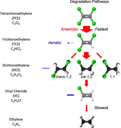
Physical processes (e.g., dilution, adsorption, and evaporation) reduce parent concentrations without generating daughter products. By contrast, microbial degradation of chlorinated solvents is complex (Figure 2) and commonly occurs by aerobic and anaerobic processes in the environment (Chu et al., 2004; Hunkeler et al., 2008). The rate of aerobic biodegradation is slow compared to anaerobic biodegradation (Morrison et al., 2006; Abe et al., 2009). Organohalide respiration is the anaerobic pathway that removes a chlorine and preferentially generates cis-1,2-dichloroethylene (DCEc12) with lower proportions of trans-1,2-dichloroethylene (DCEt12) and DCE11. A second chlorine is eventually removed by similar biochemical processes to produce VC. Eventually, microbes remove a third chlorine and generate ethene. Regardless of the exact processes, chloroethylenes dissolved in groundwater contact microbe populations and naturally become more (not less) degraded temporally and spatially.

Figure 2. PCE and TCE degradation pathways and relative rates (adapted from Morrison and Murphy, 2006). Red arrows indicate anaerobic degradation, while blue arrows indicate aerobic degradation. The size of the arrows represents the relative reaction rates.

Dechlorination is a gradual, sequential, and easily measured phenomenon using a biodegradation index for TCE (BDI_TCE). It employs the concentrations or mole fractions of TCE and its biodegradation byproducts (Table 3) determined by EPA Method 8260 to calculate the proportion of parent TCE and its byproducts DCE and VC in each sample as follows:(1) $${\mathit{BDI}}_{\mathit{TCE}}=\frac{(\mathit{DCEc}12+\mathit{DCEt}12+\mathit{DCE}11+VC)}{(\mathit{TCE}+\mathit{DCEc}12+\mathit{DCEt}12+\mathit{DCE}11+VC)}$$(1)

Table 3. Chloroethylene concentrations, biodegradation indices, and isotope ratios. Plumes from a single origin typically exhibit declining parent PCE and TCE concentrations, increasing biodegradation indices, and less negative isotope ratios. Perturbations of these trends signal boundaries between independent groundwater plumes. Units are micromole per liter (um/l), per mil (‰), standard deviation of replicate analyses (σ), and isotopic enrichment (ε) relative to Well d. Biodegradation index (BDI) is unitless that varies between 0 (no biodegradation byproducts detected) and 1 (no parent detected) as explained in the text.

Sampling Round	Well	VC um/l	DCE11 um/l	DCEc12 um/l	DCEt12 um/l	TCE um/l	PCE um/l	BDIPCE	BDITCE	BDIDCE	δ^13C ‰	σ	δ^37Cl ‰	σ	εC	εCl
1	a	0.011	0.067	0.144	0.023	5.63	ND	1.00	0.04	0.04	−22.14	0.04	0.336	0.19	1.83	1.91
1	b	1.92	0.155	5.36	ND	73.1	0.380	1.00	0.09	0.26	NA	NA	NA	NA	NA	NA
1	c	0.018	0.029	0.268	0.006	2.36	ND	1.00	0.12	0.05	−16.63	0.04	2.18	0.72	7.34	3.75
1	d	0.288	0.454	7.01	ND	601	0.446	1.00	0.01	0.04	−23.97	0.04	−1.569	0.37	0.000	0.000
1	e	0.072	0.227	1.44	0.081	52.5	0.051	1.00	0.03	0.04	−23.11	0.04	0.194	0.22	0.858	1.76
1	f	4.32	2.48	51.6	0.701	746	139	0.85	0.07	0.07	−24.99	0.04	−1.733	0.53	−1.020	−0.164
1	g	0.002	0.010	0.028	0.003	0.312	0.003	0.99	0.12	0.05	NA	NA	NA	NA	NA	NA
1	h	1.25	0.351	9.18	0.081	83.7	12.7	0.88	0.11	0.11	−25.83	0.04	−0.004	0.31	−1.858	1.56
1	i	0.320	0.227	7.43	0.040	83.7	11.5	0.89	0.09	0.04	−23.71	0.04	0.135	0.22	0.260	1.70
1	j	0.256	0.186	6.29	ND	76.1	6.33	0.93	0.08	0.04	−25.23	0.04	0.070	0.50	−1.259	1.64
1	k	0.002	0.008	0.557	0.003	3.50	0.004	1.00	0.14	0.00	−25.42	0.04	0.496	0.55	−1.453	2.06
1	l	1.76	0.629	36.1	0.134	274	0.115	1.00	0.12	0.05	−25.66	0.04	0.122	0.23	−1.693	1.69
1	m	0.042	0.085	7.22	0.113	3.81	ND	1.00	0.66	0.01	−19.49	0.04	2.81	0.42	4.48	4.38
1	n	0.018	0.029	0.268	0.006	2.36	ND	1.00	0.12	0.05	−16.63	0.04	2.18	0.72	7.34	3.75
1	p	0.056	0.064	5.16	0.066	4.64	ND	1.00	0.54	0.01	−22.21	0.08	1.31	0.84	1.76	2.88
2	d	0.688	ND	16.5	0.413	578	ND	1.00	0.03	0.04	−23.97	0.31	−1.569	0.76	0.000	0.000
2	e	0.158	0.309	10.1	0.144	44.1	0.057	1.00	0.20	0.01	−18.75	0.31	−1.716	0.30	5.22	−0.147
2	f	4.16	1.96	53.6	0.650	723	127	0.86	0.08	0.07	−24.62	0.31	−2.813	0.37	−0.650	−1.244
2	i	0.496	0.113	8.15	0.050	21.3	6.03	0.83	0.29	0.06	−22.36	0.21	−1.582	0.27	1.61	−0.013
2	k	ND	0.004	0.124	ND	2.97	0.006	1.00	0.04	0.00	NA	NA	NA	NA	NA	NA
2	l	1.92	0.609	30.9	0.113	266	0.133	1.00	0.11	0.06	−24.74	0.21	−1.755	0.17	−0.770	−0.186
2	m	0.035	0.067	6.40	0.124	2.89	ND	1.00	0.70	0.01	−16.51	0.21	1.55	0.16	7.46	3.12
2	p	0.038	0.050	8.15	0.063	2.82	ND	1.00	0.75	0.00	−20.40	0.04	−0.003	0.67	3.57	1.57
2	q	0.030	0.155	5.57	0.045	24.4	0.046	1.00	0.19	0.01	−23.92	0.21	−3.159	0.54	0.050	−1.590
2	s	ND	ND	ND	ND	ND	ND	ND	ND	ND	NA	NA	NA	NA	NA	NA
2	t	0.432	0.454	45.4	0.289	71.5	0.072	1.00	0.39	0.01	−22.64	0.21	−3.351	0.25	1.33	−1.782
2	u	0.528	0.629	11.3	0.165	98.9	0.205	1.00	0.11	0.04	−21.83	0.21	−4.059	0.05	2.14	−2.490
2	v	0.004	0.003	0.036	ND	0.259	ND	1.00	0.14	0.09	−15.17	0.31	−3.322	0.84	8.80	−1.753
2	w	0.026	0.019	0.237	ND	4.26	0.018	1.00	0.06	0.09	−23.89	0.31	−3.793	0.11	0.080	−2.224
ND	Not detected			NA	Not Analyzed

The BDI_TCE is a ratio that is scaled from 0 (no dechlorination byproducts detected) to 1 (no TCE detected). The dechlorination state can be qualitatively described as follows:

• Light dechlorination: BDI_TCE < 0.5,

• Moderate dechlorination: 0.5 < BDI_TCE < 0.9,

• Heavy dechlorination: 0.9 < BDI_TCE < 1.0, and

• Severe dechlorination: BDI_TCE = 1.0.

Reductive dechlorination is irreversible. No natural conditions will transform VC into DCE or DCE into TCE. Groundwater migrating away from its source area will degrade systematically from TCE into daughter byproducts. The appearance of groundwater with less degraded TCE (i.e., lower BDI_TCE) within downgradient groundwater plume exhibiting more degraded TCE signifies an independent release. The horizontal and vertical concentration and BDI_TCE gradients are used synoptically to differentiate TCE plumes potentially generated at different properties within the study area.

Similar indices can be constructed using alternative parent substances. For example, dry-cleaner releases can contain PCE as the primary solvent and TCE as a spot cleaner or a degradation byproduct of PCE. The BDI equation for PCE is:(2) $${\mathit{BDI}}_{\mathit{PCE}}=\frac{(\mathit{TCE}+\mathit{DCEc}12+\mathit{DCEt}12+\mathit{DCE}11+VC)}{(\mathit{PCE}+\mathit{TCE}+\mathit{DCEc}12+\mathit{DCEt}12+\mathit{DCE}11+VC)}$$(2)

The dechlorination state is qualitatively described as follows:

• Light dechlorination:BDI_PCE < 0.5,

• Moderate dechlorination:0.5 < BDI_PCE < 0.9,

• Heavy dechlorination:0.9 < BDI_PCE < 1.0, and

• Severe dechlorination:BDI_PCE = 1.0.

Some groundwater plumes only contain primary and secondary daughter products; e.g., DCE and VC, respectively. The BDI equation for this plume would be:(3) $${\mathit{BDI}}_{\mathit{DCE}}=\frac{\left(VC\right)}{(\mathit{DCEc}12+\mathit{DCEt}12+\mathit{DCE}11+VC)}$$(3)

The dechlorination state is qualitatively described as follows:

• Light dechlorination: BDI_DCE < 0.5,

• Moderate dechlorination: 0.5 < BDI_DCE < 0.9,

• Heavy dechlorination: 0.9 < BDI_DCE < 1.0, and

• Severe dechlorination: BDI_DCE = 1.0.

Forensic investigators select the most appropriate BDI index based on the project-specific objectives and range of degradation observed in a study area. BDI_PCE works well for groundwater plumes containing detectable PCE, TCE and DCE in many samples outside the source area. The BDI_TCE works well for groundwater plumes containing detectable TCE and DCE outside the source area. The BDI_DCE works well for groundwater plumes containing little to no detectable PCE or TCE outside the source area.

LOE 4: carbon isotopes

Stable isotope ratios for multi-compound contaminants (e.g., CVOCs and selected degradation byproducts) were generated using GC-IRMS (Table 4). The carbon stable isotope ratios were calculated as a less abundant, heavy stable isotope relative to the most abundant, lighter stable isotope (R_C = ¹³C/¹²C). The instrument configuration included a purge and trap concentrator, gas chromatograph, a combustion oven, and a Thermo Fisher Scientific Delta V IRMS detector (Hunkeler et al., 1999; Auer et al., 2006; Abe et al., 2009). A carrier gas transferred the VOC contaminants through a GC column, which was incrementally heated to separate the analytes based upon different vapor pressures and affinity for the stationary phase (i.e., film on the inside walls) of the GC capillary column. As each analyte eluted from the GC column, it entered a combustion oven, which operated at high temperature (e.g., 1000 °C) and housed a ceramic combustion reactor that contained a catalyst (e.g., NiO, CuO, Pt, or equivalent). Analytes were quantitatively combusted into gases (i.e., CO₂ and H₂O) inside the combustion reactor. Residual moisture was removed before the gases enter the IRMS where CO₂ molecules were subjected to electron impact ionization.

Table 4. Isotope instrument specifications used in this study.

Description	Carbon Isotopes	Chlorine Isotopes
Instrument	GC-IR/MS	GC-qMS
Purge and Trap	Tekmar Velocity XPT	Tekmar Velocity XPT
Purge Gas	Nitrogen	Helium
Gas chromatograph	Thermo Fisher Ultra Trace II	Agilent 6890
Column	J&W DB-VRX	J&W DB-VRX
Specifications	60 m x 0.25 mm	60 m x 0.25 mm x 1.4 µm
Carrier Gas (He)	Helium	Helium
Transfer line	ThermoFinnigan GC combustion III interface	250° C
Oven Program 1	Not reported	35° C for 5 minutes
Oven Program 2	Not reported	2° C/min to 120° C
Oven Program 3	Not reported	15° C/min to 220° C
Pressure	Not reported	15.75 psi
Total Flow	Not reported	33.0 mL/minute
Mass spectrometer	Thermo Fisher Scientific Delta V Plus IRMS	Agilent 5975c
Scan Rate	N/A	∼100 scans/peak

Ions were separated based on differences in mass, using magnetic sector mass analyzers. Ion currents were detected simultaneously using Faraday cup detectors. Each ion was measured simultaneously, generating very precise isotope ratios calibrated against a reference sample. Isotope ratios were expressed in “delta” notation. Sample ratios were first normalized to an international standard then multiplied by 1000. Normalization to an international standard improved laboratory comparability.(4) $${\mathrm{\delta }}^{13}C=\left[\left(\frac{R_{\mathit{sample}}}{R_{\mathit{standard}}}\right)-1\right]\mathrm{ }x\mathrm{ }1000$$(4)

Since changes or “deltas” due to isotopic discrimination are small, multiplying by 1000 results in larger numbers that are easier to analyze. Results are traditionally reported in parts per thousand, aka parts per mil (‰), which are equivalent to milliurey (mUr) proposed by Brand and Coplen (2012). The international carbon standard is Vienna Pee Dee Belemnite (VPDB) (Gröning, 2004). As an effect of normalization, isotope values in delta notation can be positive or negative numbers. Negative numbers indicate that a sample is depleted in the heavy isotope relative to the international standard.

The field samples were analyzed with various quality control parameters primarily focused on measuring stable carbon ratios with a standard deviation < 0.5 ‰ vs. VPDB for the analytical method. The analytical sequence began with multiple initial calibration standards that isotopically bracket the manufactured range of target analytes (R² > 0.95, calculated value +/- 0.5 ‰ vs. VPDB of true value). Daily continuing calibration standard runs demonstrated constant isotope ratios throughout all analytical sequences. Daily method blanks demonstrated the absence of laboratory contamination and method artifacts. Field sample duplicates were run at 20% frequency (calculated value +/- 0.5 ‰ vs. VPDB of true value) with standard deviations averaging 0.14 +/- 0.11 ‰. Practically, samples with δ¹³C that differed by more than 0.5 ‰ exceeded the total variability of the method. All lines of evidence helped determine if significant isotope differences were attributed to distinct sources or biodegradation trends.

LOE 5: chlorine isotopes

Stable chlorine isotope ratios (R_Cl = ³⁷Cl/³⁵Cl) were measured on a PT GC-qMS instrument (Table 4) operated in SIM mode (Sessions, 2006; Sakaguchi-Soder et al., 2007; Aeppli et al., 2009, 2010; Bernstein et al., 2011; Bouchard, 2014). The qMS acquisition parameters were modified to collect more than 100 mass spectral scans per chloroethylene analyte peak. By contrast standard environmental GC-qMS methods obtain 5 to 10 scans per peak (USEPA, 1996c, 2014b). The high-frequency scanning approach optimized the mass spectral resolution of the method and provided sufficient data to demonstrate improved precision of chlorine isotope measurements relative to lower GC-qMS scan rate methods.

Nominal samples sizes were 5 mL for water and 5 g for soil, which were adjusted based on conventional VOCs results. The chlorine isotope ratios of laboratory replicates varied by less than 1.0 ‰ between 80 and 1,000 ug/l in waters and 80 ug/kg to 1,000 ug/kg for soils, although the lower calibration range was extended to 30 ug/l and qualified with a “J” flag (i.e., a qualifier that indicated an estimated value) provided the initial calibration was less than 2.0 ‰ SMOC. Samples with chloroethylene compound above 1,000 ug/l or 1,000 ug/kg were diluted into the calibration range with reagent water. Techniques were also developed to run larger volume water samples (25 mL) for chloroethylene concentrations below 30 ug/l. Each sample was fortified with conventional internal standards and surrogates using an identical lot number during the study and brought up to standard volume with reagent water. Helium (99.999%) purged the target compounds from the sample at 40 °C onto a sorbent column (Supelco VOCARB K), which was subsequently heated and target analytes desorbed into the GC-qMS instrument.

The chlorine isotopic composition of TCE was measured by directly monitoring molecular ions m/z 132 (C₂H³⁷Cl³⁵Cl₂) and m/z 130 (C₂H³⁵Cl₃) and comparing chlorine isotope ratios relative to the international standard for chlorine or standard mean ocean chloride (SMOC) (Gröning, 2004; Sessions, 2006).(5) $${\mathrm{\delta }}^{37}Cl=\left[\left(\frac{R_{\mathit{sample}}}{R_{\mathit{standard}}}\right)-1\right]\mathrm{ }x\mathrm{ }1000$$(5)

The stable isotope fragments for other chlorinated compounds were measured using the molecular ion in similar fashion.

The field samples were analyzed with many quality controls primarily focused on measuring stable chlorine ratios with a standard deviation < 1.0 ‰ for the analytical method. The analytical sequence began with a multiple level initial calibration ranging in concentration from 30 ng/L to 1,000 ng/L that assured stable isotope ratio measurements over the concentration range of the calibration standards. Independent calibration verification reference samples with different origins and independently verified chlorine isotope values were analyzed after the initial calibration standards to assure isotope ratio accuracy and precision. Daily tune checks and triplicate continuing calibration standard runs demonstrated constant mass spectrometer performance and the stability of isotope ratios measured throughout the analytical sequence. Daily method blanks demonstrated the absence of laboratory contamination, method artifacts, or interference from the HCl preservative.

Currently, CSIA methods experience technical challenges. First, isotopically certified standards for all chloroethylene compounds are not available for all matrices (Gröning, 2004). Second, instrument-specific isotope fractionation can deviate slightly from the international standard (Auer et al., 2006). This study addressed these challenges with multiple strategies. First, it employed one lot of calibration standard throughout the study (Ultra Scientific, Haloethanes Standard, Part #: DWM-520-1) that was isotopically characterized by multiple isotope laboratories against the international standard. Second, it procured additional reference samples of PCE, TCE, and other CVOC solvents from independent sources that were subsequently characterized by multiple isotope laboratories and analyzed after the initial instrument calibration to confirm the accuracy and precision of the chlorine isotope calibration. Third, field samples were isotopically bracketed by continuing calibration standard run every 12 hours to evaluate isotopic drift and calculate isotopic ratios in all subsequent QC and field samples. Fourth, a reference field groundwater sample (Well d) with stable concentration and chemical biodegradation state was analyzed with every initial calibration to assure measurement precision throughout the two year study period.

Repeated analyses of the reference samples collected from Well d demonstrated small differences in δ¹³C and δ³⁷Cl between sampling events attributed to the use of different instruments and initial calibrations over time. In order to maximize comparability between sampling rounds, a correction factor was applied.(6) $${\delta }^{13}{C}_{Sx\mathrm{ }Ex\mathrm{ }\mathit{Corrected}}={\delta }^{13}{C}_{Sx\mathrm{ }Ex}+({\delta }^{13}{C}_{\mathit{Sref}\mathrm{ }\mathit{Eref}}-{\delta }^{13}{C}_{\mathit{Sref}\mathrm{ }Ex})$$(6) where,

SxEx Field sample x (Sx) collected during secondary sampling event (Ex),

SrefE0 Reference sample (Sref) collected during reference sampling event (Eref), and

SrefEx Reference sample (Sref) collected during secondary sampling event (Ex).

An analogous equation applies for chlorine. These correction factors improved comparability of data between the two sampling events and helped assure measurement accuracy and precision throughout the study.

Source signatures that differed more than the method precision, provided a scientific basis for differentiating impacts from multiple candidate sources or significant changes attributed to biodegradation. Replicate sample analyses provided a practical reference for demonstrating the total method precision. In this study, all field samples were measured in triplicate for δ³⁷Cl with standard deviations averaging 0.41 +/- 0.26 ‰. Practically, samples with δ³⁷Cl that differed by more than 1.0‰ exceeded the variability of the method. All lines of evidence helped determine if significant isotope differences were attributed to distinct sources or biodegradation trends.

The isotopic enrichment (ε) of chlorine and carbon during organohalide respiration has been observed in the field and confirmed in the laboratory (Hunkeler et al., 2008; Brand and Coplen, 2012; Heckel et al., 2018; Lihl et al., 2019). Isotope enrichment is calculated as the difference of an isotope ratio in time (e.g., the beginning and end of an organohalide respiration study) or space (e.g., the source area and downgradient area of impact).(7) $${\epsilon }_C=\left({\delta }^{13}{C}_a-{\delta }^{13}{C}_b\right)\mathrm{*}1000$$(7) where,

1. Sample at time x or downgradient location x, and

2. Sample at time 0 (start) or source location.

An analogous equation applies for chlorine. The correlation of dual stable isotopes provides a slope that reflects the magnitude of the compound-specific isotope effect:(8) $${\Lambda }_{C/Cl}=\frac{({\delta }^{13}{C}_a-{\delta }^{13}{C}_b)}{({\delta }^{37}{Cl}_a-{\delta }^{37}{Cl}_b)}\approx \mathrm{ }\frac{{\epsilon }_C}{{\epsilon }_{Cl}}$$(8)

Heckel et al. (2018) proposed that addition protonation and addition elimination explained how specialized degrader strains from Dehalococcoidia class bacteria described in previous studies (e.g., certain Dehalococcoides mccartyi and Dehalogenimonas) completely metabolized chloroethylenes to ethene, while dechlorination by other microorganisms (e.g., Geobacter lovleyi) only partially metabolized chloroethylenes to cis-DCE. Heckel et al. (2018) used dual isotope enrichment plots, ε_Cl verses ε_C with slope Λ_C/Cl to demonstrate the interrelationship between reaction rates, product formation, enzymes, and isotope changes (3.9 < Λ_C/Cl < 18). Lihl et al. (2019) used dual isotope enrichment plots (2.3 < Λ_C/Cl < 18) to demonstrated differences between the microbial dechlorination of structurally distinct chloroethylenes (i.e., PCE, TCE, and cis-DCE) to evaluate the metabolic addition-elimination mechanisms in pure cultures of selected bacteria and demonstrated the significance of microbial pre-cultivation to bridge the gap between laboratory studies and contaminant removal from the environment. This study employed the Λ_C/Cl metrics as a forensic signature to evaluate the nature of biodegradation observed in the study area.

Results and discussion

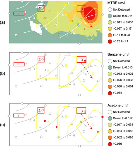
Chloroethylene concentrations across the study area generally declined from the source areas to the tributary flowing along the southern edge of the study area (Figure 3). Colored circles (i.e., post plots) depicted the changing groundwater concentrations from well to well. The interpolated surfaces were kriged to help visualize the general trends using the post plot color symbology with greatest statistical significance within approximately 150 ft (46 m) of most monitoring wells (Stout et al., 2017). Elevated PCE concentrations (Figure 3a) centered around Source Area 2 (dry cleaner) with gradually declining concentrations through Downgradient Zones A and B. Elevated TCE concentrations (Figure 3b) centered around Source Areas 1 (metal fabricator) and 2 (dry cleaner) with gradually declining concentrations through Downgradient Zones A and B. Within the eastern third of the study area, the highest TCE concentrations centered around Source Area 3 (auto service station) with declining concentrations through Downgradient Zone C. Detections of methyl-t-butyl ether (MTBE – a gasoline oxygenate additive) and benzene near Source 3 further demonstrated historical gasoline releases associated with automobile operations (Figures 4a and b, respectively). Detections of household solvents, like acetone (Figure 4c), largely occurred in downgradient zones and likely demonstrated chronic localized releases with no spatial association with chloroethylene plumes attributed to Sources 1, 2, or 3. The first-generation biodegradation breakdown products dominated by DCEc12 (Figure 3c) similarly declined from Sources 1, 2, and 3 through the Downgradient Zones towards the tributary. The second-generation breakdown product, VC (Figure 3d), occurred at greatest concentrations below Source Area 2 before declining on a southeasterly gradient suggesting greater anaerobic dechlorination from the chloroethylene plume originating at the dry cleaner facility. These spatial concentration gradients (LOE 1) help confirm the southeasterly groundwater flow; however, the degree to which Source Area releases commingled in the Downgradient Zones was unclear based upon LOE 1 alone.

Figure 3. Spatial projection of chloroethylene concentrations and interpolated surfaces (um/l): (a) PCE, (b) TCE, (c) DCEc12, and (d) VC. Candidate source areas (red outline), Downgradient Zones (yellow outline), and piezometric contours from Figure 1.

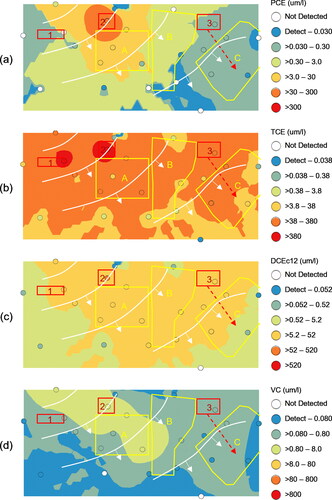
Figure 4. Spatial projection of other VOC concentrations and interpolated surfaces (um/l): (a) MTBE, (b) benzene, and (c) acetone. Candidate source areas (red outline), Downgradient Zones of concern (yellow outline), and piezometric contours from Figure 1.

Non-target compounds confirmed historical releases from Sources 2 and 3 (LOE 2). Dense NAPL was recovered from the bottom of the soil boring, which was eventually developed into Well f near Source 2 (Figure 1b). A high-resolution hydrocarbon fingerprint (GC/FID with compound confirmation by GC-qMS) of the DNAPL sample exhibited PCE commingled with multiple petroleum products (Figure 5a). Stoddard solvent eluted between n-octane (n-C₈) and n-tridecane (n-C₁₃). The co-occurrence of Stoddard solvent and PCE represented two dry cleaning solvents likely used at the dry cleaner facility between 1928 to 1950s and 1940s to 1990s, respectively (Doherty, 2000). The mineral oils eluting between n-C₁₃ and n-tetracontane (n-C₄₀) were attributed to oil and grease removed by the dry-cleaning fluids. The absence of this NTC signature outside the Well f sampling location demonstrated no significant DNAPL mobility towards proximal locations. Practically, these data suggested that a remedy focused on reducing dissolved chloroethylenes in groundwater would be possible once the DNAPL source material was mitigated.

Figure 5. Non-target compounds in solvent extracted soil samples: (a) MW-f collected at bedrock (34 ft) and analyzed by GC/FID and (b) MW- t collected at the groundwater interface (13 ft) and analyzed using GC/FID to generate high-resolution hydrocarbon fingerprints. Compound identification was confirmed by GC/MS confirmation analyses.

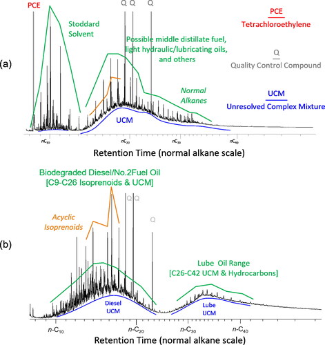
Additional NTC detections occurred within the soil boring eventually developed into Well t near Source 3 (Figure 1b). Specifically, elevated PID readings within 3 ft (0.9 m) of the groundwater interface produced hydrocarbon fingerprints of multiple petroleum products (Figure 5b). Diesel or No. 2 fuel oil eluted between n-C₈ and n-C₂₆, while lube or motor oil range eluted after n-C₂₆. These hydrocarbon products are consistent with historical releases from an automotive service station that initially accumulated as light NAPL (LNAPL) at the groundwater interface. The absence of these hydrocarbon signatures in soils and groundwater samples from proximal wells indicated little to no off-site LNAPL migration. Chloroethylenes were not detected in these soil samples, which suggested historical TCE releases from Source 3 occurred independently through a pipe or drywell below the surficial or shallow hydrocarbons observed in Figure 5b.

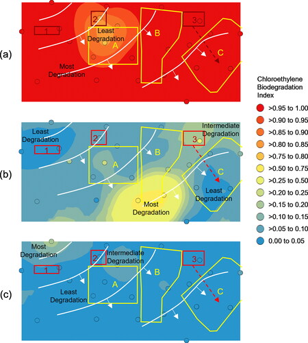
The BDI plots helped delineate the plumes of dissolved chloroethylenes. As noted previously, the only significant PCE detections occurred around Source 2 (Figure 6a) which exhibited a slightly enriched footprint (BDI_PCE > 0.75) that migrated south into Downgradient Zone A with a radial geometry that almost reached Downgradient Zone B with no detectable impacts in Downgradient Zone C. The highest proportions of TCE relative to DCE and VC (BDI_TCE < 0.05) occurred around Source Area 1 and at the end of an historical drainage feature emanating from Source Area 3 (Figure 6b). Source 2 also exhibited relatively fresh TCE (BDI_TCE < 0.10). TCE degradation increased in a southeasterly direction from Sources 1 and 2 to a collection area at the southern end of Downgradient Zone B where biodegradation accelerated (BDI_TCE > 0.50). Importantly, TCE impacted groundwater below Downgradient Zone C exhibited less biodegradation than groundwater to its north and west signifying little to impact from these directions. In this case study, the BDI_DCE was very uniform due to the extremely low proportion of VC relative to DCE isomers (Figure 6c). The spatial BDI_DCE patterns demonstrated that the CVOCs in groundwater below Source 2 exhibited greater degradation than groundwater near Sources 1 and 3. Collectively the BDI patterns (LOE 3) suggested the chloroethylene plumes from Sources 1 and 2 migrated and degraded through Downgradient Zones A and B, but were too degraded to account for the fresher chloroethylene pattern in Downgradient Zone C. Therefore, the BDI_TCE pattern demonstrated that Source 3 was the source of chloroethylenes in Downgradient Zone C.

Figure 6. Spatial projections of trichloroethylene biodegradation indices: (a) PCE degradation Index, (b) TCE degradation index, and (c) DCE degradation index. Candidate source areas (red outline), Downgradient Zones of concern (yellow outline), and piezometric contours from Figure 1.

A subset of the compliance testing samples with TCE concentrations above approximately 30 ug/l fell within the quantification range of the isotope testing methods. The lowest carbon isotope value for TCE was observed downgradient of the Source 3 historical drainage feature below Downgradient Zone C and this feature extended west to Downgradient Zone B (Figure 7a). Sources 1 and 2 exhibited slightly higher (heavier) TCE δ¹³C values which extended to Downgradient Zones A and B. These results indicated a mixing zone below Downgradient Zone B of TCE from Sources 2 and 3 with possible contributions from Source 1.

Figure 7. Spatial projections of compound specific isotope ratios and interpolated surfaces: TCE δ¹³C ‰ and (b) TCE δ³⁷Cl ‰. Candidate source areas (red outline), Downgradient Zones (yellow outline), and piezometric contours from Figure 1.

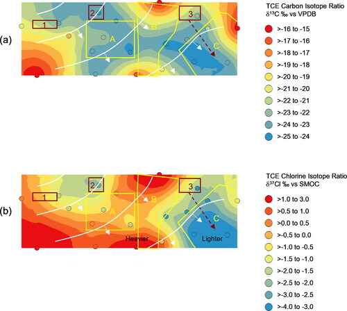
The TCE δ³⁷Cl value was lowest below Downgradient Zone C downgradient of the Source 3 drainage feature (Figure 7b). Slightly higher TCE δ³⁷Cl values occurred proximal to Sources 1 and 2. This observation confirmed distinct isotopic signatures for the TCE associated with each source area (1&2-heavier vs. 3-lighter). The integrated TCE δ³⁷Cl signature became gradually enriched due to microbial dechlorination as the groundwater spread radially out of the source areas and migrated to the southeast. Sources 1 and 2 likely impacted groundwater below Downgradient Zones A and B; however, the absence of heavier TCE δ³⁷Cl ratios in Downgradient Zone C indicated no discernable impact from Sources 1 and 2. These data further suggested that the prevailing southeasterly groundwater flow from Sources 1 and 2 migrated to the heavily biodegraded TCE pool south of Downgradient Zone B before discharging into the tributary with no significant easterly flow to Downgradient Zone C.

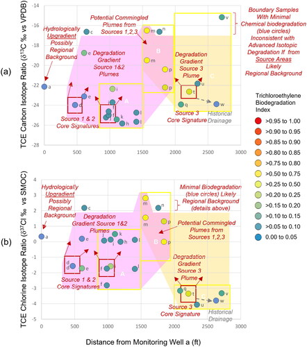
A multivariate approach provided further insights concerning the origin and fate of dissolved chloroethylenes in the study area. Replotting the spatial dimension on the x-axis (i.e., distance from Well a) provided an east-west gradient for comparing isotope ratios on the y-axis and TCE BDI by symbology color. This plot demonstrated that groundwater from Sources 1 and 2 failed to reach Downgradient Zone C. Specifically, the dramatic shift towards isotopically enriched carbon and chlorine isotope ratios for biodegraded TCE in Downgradient Zones A and B is clear for most samples on both the δ¹³C (Figure 8a) and δ³⁷Cl (Figure 8b) plots. This trend was not apparent among the TCE δ¹³C ratios associated with groundwater from Wells h, j, k, and l possibly due to the type of organohalide respiration occurring in groundwater or the influence of proximal NAPL containing waste oils. Nevertheless, these plots illustrated the different isotope signatures between Sources 1 and 2 (enriched) and Source 3 (depleted). The absence of Source 1 and 2 impacts in Downgradient Zone C was especially clear in the significant difference between the TCE δ³⁷Cl ratios. Specifically, the isotopic signatures of TCE Sources 1 and 2 (-2 > TCE δ³⁷Cl < −1) exhibited biodegradation as TCE migrated through Downgradient Zone A (-2 > TCE δ³⁷Cl < 1) and biodegraded further as TCE migrated through Downgradient Zone B (0 > TCE δ³⁷Cl < 2). The isotopically light TCE signatures observed in Downgradient Zone C (TCE δ³⁷Cl < −3) rules out meaningful contributions of enriched TCE sources from the west. By contrast, the isotopic signatures associated with Source 3 that migrated to Downgradient Zone C could potentially biodegrade, become isotopically heavier and explain the TCE detections in Downgradient Zone B. Hydrologically, the pathway from Source 3 to Downgradient Zone B would likely result from radial flow similar to the PCE footprint around Source 2. Interestingly, limited chemical biodegradation and extremely enriched isotopic signature in boundary Wells a, c and n were inconsistent with biodegraded releases from Sources 1, 2, and 3; rather, these features indicated a regional TCE background with concentrations below applicable regulatory limits.

Figure 8. Spatial projection of compound specific isotope ratios with distance from Well a: (a) TCE δ¹³C ‰ and (b) TCE δ³⁷Cl ‰ on a spatial gradient calculated as sample distance from MW-a. Candidate source areas (red outline) and Downgradient Zones (yellow outline) from Figure 1. Chloroethylene degradation symbology from Figure 4. Downgradient Zone A was likely impacted by metal fabricator (Source 1) and dry cleaner (Source 2). Downgradient Zone C was likely impacted by service station (Source 3) with no impact from Sources 1&2 evidenced by heavier TCE δ³⁷Cl. Downgradient Zone B potentially impacted by Sources 1,2,3. Regional background observed at MW-a, -c, and –n.

Dual isotope enrichment plots demonstrated good agreement between the organohalide respiration signatures observed in this case study and organohalide respiration studies featuring known bacterial species and controlled experimental conditions (Figure 9). The slope (Λ_C/Cl) of carbon enrichment (ε_C = [δ13C_{Well x} – δ13 C_{Well d}]) and chlorine enrichment (ε_Cl = [δ³⁷Cl_{Well x} – δ³⁷Cl_{Well d}]) was calculated with the conservative assumption that TCE was only released from Source 1 represented by groundwater collected from Well d. This framework demonstrated that the attribution of groundwater impacts in Area C to the historical release at Well d was not supported by the data as evidenced by the isotopically lighter groundwater from Area C, because negative TCE chlorine enrichment (ε_Cl < 0 or Λ_C/Cl < 0) is not possible; hence, groundwater from Area C is inconsistent with groundwater from Well d, Area A, and Area B. The negative TCE chlorine enrichment is also not possible given the increasingly positive TCE chlorine enrichment in groundwater moving through Areas A and B before any potential contact with Area C.

Figure 9. Isotopic enrichment (ε) of TCE chlorine and carbon isotopes: Dual isotope enrichment plots help compare field observations to published biodegradation studies using known bacterial species capable of organohalide respiration in controlled experimental conditions. The slope (Λ_C/Cl) of chlorine enrichment (ε_Cl = [δ³⁷Cl_{Well x} – δ³⁷Cl_{Well d}]*1000) and carbon enrichment (ε_C = [δ¹³C_{Well x} – δ¹³C_{Well d}]*1000) hypothetically assumed TCE was only released from Source 1 represented by groundwater collected from Well d. This conclusion was not supported by the data as evidenced by the isotopically lighter groundwater from Area C (ε_Cl < 0). However, the range of Λ_C/Cl of 1.3, 2.4, and 2.6 observed herein were consistent with the several distinct microcosm studies and suggested multiple microbiomes may control TCE degradation in different parts of the study area.

The range of Λ_C/Cl observed between selected source and downgradient areas were consistent with the several distinct laboratory dechlorination studies (Figure 9). The Λ_C/Cl between Source 1 (Well d) and groundwater from Area A during the first sampling event (Λ_C/Cl = −0.44) was not surprising given the lack of significant organohalide respiration (0.01 > BDI_TCE < 0.12). However, the higher ε_Cl relative to ε_C among the Area A samples from the first event suggested the onset of chlorine isotope enrichment (ε_Cl) preceded carbon isotope enrichment (ε_C) among these samples. Alternatively, groundwater contaminated by Sources 1 or 2 could have migrated through Area A without significant degradation followed by significant dechlorination (0.08 > BDI_TCE < 0.75) during its migration through Area B with a commensurate increase in isotopic enrichment (Λ_C/Cl = 2.6). This degree of degradation agreed with the Λ_C/Cl between Source 2 (Well f) and groundwater from Area A during the second sampling event (Λ_C/Cl = 2.4). Consequently, Sources 1 (Well d) and 2 (Well f) remained potential sources of groundwater impacts in Area A. Both of these isotopic signatures compared well with the TCE degradation study using the Donna II culture with Dehalococcoides mccartyi (Λ_C/Cl = 2.3 ± 0.1) or the KB-1 RF culture also containing D. mccartyi (Λ_C/Cl = 2.7 ± 0.2) reported by Lihl et al. (2019).

The isotopic enrichment among samples from Source 3 represented by Well t and groundwater around Area C varied considerably and exhibited a slightly positive slope (Λ_C/Cl = 1.8). Groundwater samples collected from Wells t, u, w, and q contained isotopically lighter TCE compared to groundwater collected from Areas A and B. Groundwater from Well v differed significantly, which suggested an independent release compared to other Area C groundwater samples. These observations suggested that a portion of the historical offsite discharge preferentially migrated via pipe or natural drainage feature to Area C. The exact preferential migration pathway between Source t and Area C was unknown as were the bacteria species in the aquifer. Site investigators may focus on these issues should these details prove important in the future.

Conclusions

Multiple lines of evidence offered improved resolution of chloroethylene impacts in a groundwater aquifer with multiple candidate sources that historically released PCE and TCE. Spatial projections of chloroethylene concentrations, non-target analytes, biodegradation indices, carbon isotope ratios, and chlorine isotope ratios helped isolate contaminant source signatures and track their increasingly weathered signatures through portions of the study area. Chemical fingerprinting and CSIA data demonstrated that Downgradient Zones A and B were impacted by historical releases from Sources 1 and 2, while clarifying that a Downgradient Zone C was impacted exclusively by Source 3. These data also demonstrated the presence of a low-level regional TCE groundwater plume and provided insights on the prevailing direction of groundwater flow.

The multiple lines of evidence approach described in this paper helped distinguish chlorinated solvent impacts better than over-reliance on any one individual metric. Target and NTC analyte patterns demonstrated independent releases occurred at all three source areas, while helping delineate the outer boundaries of the area of impact. The spatial patterns of carbon and chlorine isotopes were needed to resolve the boundary between at least two groundwater plumes. Distinct isotope enrichment trends within the study area further demonstrated that organohalide respiration in the laboratory studies were consistent with field observations, albeit with weaker isotope enrichment trends (1.3 < Λ_C/Cl < 2.6). This observation suggested that natural organohalide respiration can be monitored and possibly enhanced as the metabolic processes are better understood. The range of isotopic enrichment within the study area suggested the chloroethylene impacted groundwater travelled through a mosaic of different microbiomes, which sequentially reduced contaminant concentrations, altered isotopic signatures, and created a trail for forensic investigators to follow.

Acknowledgements

We thank James Occhialini, Susan O’Neil, John Trimble, Andrew Rezendes, Andrew Cram and the entire chemistry team at Alpha Analytical with facilities in Mansfield, MA and Westborough, MA which conducted the VOC, high resolution hydrocarbon fingerprinting, non-target compound scan, and chlorine CSIA analyses. We also thank our colleagues at Pace Analytical in Pittsburgh, PA which conducted the carbon CSIA analyses. We thank our colleague Bo Liu at NewFields for interpolating the data presented in many figures.

Declaration of interest statement

This work was sponsored by the former owner of Source 1 (metal fabricator) in support of confidential and settled arbitration proceedings.

References

- Abe, Y., Aravena, R., Zopfi, J., Shouakar-Stash, O., Cox, E., Roberts, J. D., et al. 2009. Carbon and chlorine isotope fractionation during aerobic oxidation and reductive dechlorination of vinyl chloride and cis-1,2-dichloroethene. Environmental Science & Technology 43 (1):101–107.
- Aeppli, C., Berg, M., Cirpka, O. A., Holliger, C., Schwarzenbach, R. P., and Hofstetter, T. B. 2009. Influence of mass-transfer limitations on carbon isotope fractionation during microbial dechlorination of trichloroethene. Environmental Science & Technology 43:8813–8820.
- Aeppli, C., Holmstrand, H., Andersson, P., and Gustafsson, O. 2010. Direct compound-specific stable chlorine isotope analysis of organic compounds with quadrupole GC/MS using standard isotope bracketing. Analytical Chemistry 82:420–426.
- Agency for Toxic Substances and Disease Registry. 1996. Toxicological Profile for 1,2-Dichloroethene. In 198. U.S. Department of Health and Human Services.
- Agency for Toxic Substances and Disease Registry. 2006. Toxicological Profile for Vinly Chloride. In 329. U.S. Department of Health and Human Services.
- Agency for Toxic Substances and Disease Registry. 2019a. Toxicological Profile for 1,1-Dichloroethene. In 263. U.S. Department of Health and Human Services.
- Agency for Toxic Substances and Disease Registry. 2019b. Toxicological Profile for Tetrachloroethylene. In 435. U.S. Department of Health and Human Services.
- Agency for Toxic Substances and Disease Registry. 2019c. Toxicological Profile for Trichloroethylene. In 511. U.S. Department of Health and Human Services.
- Aller, L., Bennett, T. W., JHackett, G., Petty, R. J., Lehr, J. H., Sedoris, H., et al. 1991. Handbook of Suggested Practices for the Design and Installation of Ground-Water Monitoring Wells. Vol. EPA 160014-891034. Environmental Monitoring Systems Laboratory.
- American Society for Testing and Materials. 2016. Standard practice for design and installation of groundwater monitoring wells. West Conshohocken, PA USA: American Society for Testing and Materials ASTM Method D5092/D5092M - 16.
- Auer, N. R., Manzke, B. U., and Schulz-Bull, D. E. 2006. Development of a purge and trap continuous flow system for the stable carbon isotope analysis of volatile halogenated organic compounds in water. Journal of Chromatography. A 1131 (1–2):24–36.
- Beneteau, K. M., Aravena, R., and Frape, S. K. 1999. Isotopic characterization of chlorinated solvents–laboratory and field results. Organic Geochemistry 30 (8A):739–753.
- Bernstein, A., Shouakar-Stash, O., Ebert, K., Laskov, C., Hunkeler, D., Jeannottat, S., et al. 2011. Compound-specific chlorine isotope analysis: A comparison of gas chromatography/isotope ratio mass spectrometry and gas chromatography/quadrupole mass spectrometry methods in an interlaboratory study. Analytical Chemistry 83:7624–7634.
- Bouchard, D. 2014. δ13C and δ37Cl on gas-phase TCE for source identification investigation - innovative solvent-based sampling method. In Environmental Forensics: Proceedings of the 2014 INEF Conference, Cambridge, UK, 13 pp.
- Brand, W. A., and Coplen, T. B. 2012. Stable isotope deltas: tiny, yet robust signatures in nature. Isotopes in Environmental and Health Studies 48 (3):393–409.
- Chu, K.-H., Mahendra, S., Song, D. L., Conrad, M. E., and Alvarez-Cohen, L. 2004. Stable carbon isotope fractionation during aerobic biodegradation of chlorinated ethenes. Environmental Science & Technology 38 (11):3126–3130.
- Doherty, R. E. 2000. A history of the production and use of carbon tetrachloride, tetrachloroethylene, trichloroethylene and 1,1,1-trichloroethane in the United States: Part 1 – historical background; carbon tetrachloride and tetrachloroethylene. Environmental Forensics 1 (2):69–81.
- Douglas, G. S., Emsbo-Marringly, S. D., Stout, S. A., Uhler, A. D., and McCarthy, K. J. 2015. Hydrocarbon fingerprinting methods. In Introduction to Environmental Forensics, eds. Murphy, B. L. and Morrison, R. D. Boston, MA: Adademic Press, 201–309.
- Elsner, M., Jochmann, M. A., Hofstetter, T. B., Hunkeler, D., Bernstein, A., Schmidt, T. C., et al. 2012. Current challenges in compound-specific stable isotope analysis of environmental organic contaminants. Analytical and Bioanalytical Chemistry 403 (9):2471–2491.
- Gröning, M. 2004. "Chapter 40 - International stable isotope reference materials. In Handbook of Stable Isotope Analytical Techniques, ed. de Groot, P. A. Amsterdam: Elsevier, 874–906.
- Heckel, B., McNeill, K., and Elsner, M. 2018. Chlorinated ethene reactivity with Vitamin B12 is governed by cobalamin chloroethylcarbanions as crossroads of competing pathways. ACS Catalysis 8:3054–3066.
- Holt, B. D., Sturchio, N. C., Abrajano, T. A., and Heraty, L. J. 1997. Conversion of chlorinated volatile organic compounds to carbon dioxide and methyl chloride for isotopic analysis of carbon and chlorine. Analytical Chemistry 69 (14):2727–2733.
- Horst, A., Renpenning, J., Richnow, H.-H., and Gehre, M. 2017. Compound specific stable chlorine isotopic analysis of volatile aliphatic compounds using gas chromatography hyphenated with multiple collector inductively coupled plasma mass spectrometry. Analytical Chemistry 89:9131–9138.
- Hunkeler, D., Araveba, R., and Butler, B. J. 1999. Monitoring microbial dechlorination of tetrachloroethene (PCE) in groundwater using compound-specific stable carbon isotope ratios: Microcosm and field studies. Environmental Science & Technology 33 (16):2733–2738.
- Hunkeler, D., Meckenstockl, R. U., Lollar, B. S., Schmidt, T. C., and Wilson, J. T. 2008. A Guide for Assessing Biodegradation and Source Identification of Organic Ground Water Contaminants Using Compound Specific Isotope Analysis (CSIA). Ada, OK: U.S. EPA, Office of Research and Development.
- Jendrzejewski, N., Eggenkamp, H. G. M., and Coleman, M. L. 2001. Characterisation of chlorinated hydrocarbons from chlorine and carbon isotopic compositions: Scope of application to environmental problems. Applied Geochemistry 16:1021–1031.
- Jin, B., Laskov, C., Rolle, M., and Haderlein, S. B. 2011. Chlorine isotope analysis of organic contaminants using GC-qMS: Method optimization and comparison of different evaluation schemes. Environmental Science & Technology 45:5279–5286.
- Jochmann, M. A., and Schmidt, T. C. 2013. Compound-specific stable isotope analysis. Analytical and Bioanalytical Chemistry 405:2753–2754.
- Kuder, T., Van Breukelen, B. M., Vanderford, M., and Philp, P. 2013. 3D-CSIA: Carbon, chlorine, and hydrogen isotope fractionation in transformation of TCE to ethene by a Dehalococcoides culture. Environmental Science & Technology 47:9668–9677.
- Leys, D., Adrian, L., and Smidt, H. 2013. Organohalide respiration: microbes breathing chlorinated molecules. Philosophical Transactions of the Royal Society of London. Series B, Biological Sciences 368:20120316.
- Lihl, C., Douglas, L. M., Franke, S., Pérez-de-Mora, A., Meyer, A. H., Daubmeier, M., et al. 2019. Mechanistic dichotomy in bacterial trichloroethene dechlorination revealed by carbon and chlorine isotope effects. Environmental Science & Technology 53:4245–4254.
- Lollar, B. S., Slater, G. F., Ahad, J., Sleep, B., Spivack, J., Brennan, M., et al. 1999. Contrasting carbon isotope fractionation during biodegradation of trichloroethylene and toluene: implications for intrinsic bioremediation. Organic Geochemistry 30 (8A):813–820.
- Meckenstock, R. U., Morasch, B., Griebler, C., and Richnow, H. H. 2004. Stable isotope fractionation analysis as a tool to monitor biodegradation in contaminated acquifers. Journal of Contaminant Hydrology 75 (3–4):215–255. doi:.
- Meier-Augenstein, W. 1999. Applied gas chromatography coupled to isotope ratio mass spectrometry. Journal of Chromatography. A 842 (1):351–371. doi:.
- Morrison, R. D., Murphy, B. L., and Doherty, R. E. 2006. Chlorinated solvents. In Environmental Forensics: A Contaminant Specific Guide, eds. Morrison, R. D. and Murphy, B. L. Burlington, MA: Elsevier Academic Press, 259–278.
- National Library of Medicine. 2021. Hazardous substance data bank. https://www.nlm.nih.gov/toxnet/index.html.
- Numata, M., Nakamura, N., Koshikawa, H., and Terashima, Y. 2002. Chlorine isotope fractionation during reductive dechlorination of chlorinated ethenes by anaerobic bacteria. Environmental Science & Technology 36 (20):4389–4394.
- Pankow, J. F., and Cherry, J. A. 1996. Dense Chlorinated Solvents and Other DNAPLs in Groundwater: History, Behavior, and Remediation. Hove, UK: Waterloog Press.
- Renpenning, J., Hitzfeld, K. L., Gilevska, T., Nijenhuis, I., Gehre, M., and Richnow, H.-H. 2015. Development and validation of an universal interface for compound-specific stable isotope analysis of chlorine (37Cl/35Cl) by GC-high-temperature conversion (HTC)-MS/IRMS. Analytical Chemistry 87:2832–2839.
- Renpenning, J., Horst, A., Schmidt, M., and Gehre, M. 2018. Online isotope analysis of 37Cl/35Cl universally applied for semi-volatile organic compounds using GC-MC-ICPMS. Journal of Analytical Atomic Spectrometry 33:314–321.
- Sakaguchi-Soder, K., Jager, J., Grund, H., Matthaus, F., and Schuth, C. 2007. Monitoring and evaluation of dechlorination processes using compound-specific chlorine isotope analysis. Rapid Communications in Mass Spectrometry : RCM 21:3077–3084.
- Sessions, A. L. 2006. Isotope-ratio detection for gas chromatography. Journal of Separation Science 29:1946–1961.
- Shouakar-Stash, O., Frape, S. K., and Drimmie, R. J. 2003. Stable hydrogen, carbon and chlorine isotope measurements of selected chlorinated organic solvents. Journal of Contaminant Hydrology 60:211–228.
- Shouakar-Stash, O., Zhang, R. J., Drimmie, M., and Frape, S. K. 2006. Compound-specific chlorine isotope ratios of TCE, PCE and DCE isomers by direct injection using CF-IRMS. Applied Geochemistry 21:766–781.
- Slater, G. F., Lollar, B. S., Sleep, B. E., and Edwards, E. A. 2001. Variability in carbon isotopic fractionation during biodegradation of chlorinated ethenes: implications for field applications. Environmental Science & Technology 35 (5):901–907.
- Stout, S. A., Rouhani, S., Liu, B., Oehrig, J., Ricker, R. W., Baker, G., et al. 2017. Assessing the footprint and volume of oil deposited in deep-sea sediments following the deepwater horizon oil spill. Marine Pollution Bulletin 114:327–342.
- USEPA. 1996a. Method 5030B Purge-and-Trap for Aqueous Samples. Final Update III to the Third Edition of the Test methods for Evaluating Solid Waste, Physical/Chemical Methods. In EPA publication SW-846.
- USEPA. 1996b. Method 5035 Closed-System Purge-and-Trap and Extraction for Volatile Organics in Soil and Waste Samples. Final Update III to the Third Edition of the Test Methods for Evaluating Solid Waste, Physical/Chemical Methods. In EPA publication SW-846.
- USEPA. 1996c. Method 8260B Volatile Organic Compounds by Gas Chromatography/Mass Spectrometry (GC/MS). Final Update III to the Third Edition of the Test Methods for Evaluating Solid Waste, Physical/Chemical Methods. In EPA publication SW‐846.
- USEPA. 2014a. Method 5021A Closed-System Purge-and-Trap and Extraction for Volatile Organics in Soil and Waste Samples. Final Update V to the Third Edition of the Test Methods for Evaluating Solid Waste, Physical/Chemical Methods." In EPA publication SW‐846.
- USEPA. 2014b. Method 8270D Semivolatile Organic Compounds by Gas Chromatography/Mass Spectrometry (GC/MS). Final Update V to the Third Edition of the Test Methods for Evaluating Solid Waste, Physical/Chemical Methods." In EPA publication SW‐846.
- van Warmerdam, E. M., Frape, S. K., Aravena, R., Drimmie, R. J., Flatt, H., and Cherry, J. A. 1995. Stable chlorine and carbon isotope measurements of selected chlorinated organic solvents. Applied Geochemistry 10:547–552.
- Wiegert, C., Aeppli, C., Knowles, T., Holmstrand, H., Evershed, R., Pancost, R. D., et al. 2012. Dual carbon-chlorine stable isotope investigation of sources and fate of chlorinated ethenes in contaminated groundwater. Environmental Science & Technology 46:10918–10925.