Application of near infrared spectroscopy in sub-surface monitoring of petroleum contaminants in laboratory-prepared soils

ABSTRACT

This study was conducted to determine the suitability of near-infrared (NIR) spectroscopy for subsurface monitoring of crude oil contaminants in different soil types under different moisture conditions. Calibration tests, carried out in both wet and dry soils, with crude oil contents 5–30% indicate an inverse relationship between spectra and oil content with R² values ≥0.98 for dry soil mixtures. A derived index termed “Oil Index” was generated by calculating a spectral ratio between the main oil peak in the NIR region and a spectrally inactive part of the spectrum within the visible region. It was used in a series of experiments designed to test whether NIR probes could yield useful information about the movement of oil through different soils. Synthetic crude oil was dropped into a series of soil samples of different particle size distribution and moisture content. Analyses of the 3D distribution of values of the Oil Index demonstrate that it is possible to estimate and map synthetic crude oil concentration in the subsurface of the soil samples. Results showed that while the Oil Index provided a reasonable estimation for oil concentration in dry samples, this was not the case for wet samples, although the Index was useful in understanding the pattern of movement of oil contaminant in wet soils. The work indicates that this technique may enhance field investigation of oil contamination, providing an accurate in-field technique.

KEYWORDS:

• NIR spectroscopy
• crude oil
• soil contamination
• depth-probe
• Oil Index

1. Introduction

Chemical contamination is a significant environmental issue in many locations where petroleum is produced, stored, or distributed (Wartini, Malone, and Minasny 2017). It may affect the health of vegetation (Buzmakov, Egorova, and Gatina 2019; Mendelssohn et al. 2012) and modify soil characteristics (Townsend, Prince, and Suflita 2003; Wang, Feng, and Zhao 2010; Wang et al. 2013). Understanding the 3D distribution of the oil as it fills available pore spaces in the ground is an important consideration for any land mitigation or remediation.

Surveys to detect, quantify, and monitor oil movement on different substrates (soil and water) are normally done using conventional invasive ground investigation techniques, such as boreholes, sampling, and associated laboratory testing. Although these approaches construct a robust geochemical characterization of contamination, they can be expensive, require safe disposal of used samples, and provide only a discontinuous sampling. Surface geophysics is also effective. Electrical Resistivity Tomography (ERT) surveying, either on its own or in combination with other geophysical techniques, is a proven method for oil contamination investigation (Cassiani et al. 2014; Coria et al. 2009; Delgado-Rodríguez et al. 2014; Ioane et al. 1999). The principle used is to delineate contaminated sites based on readings of apparent resistivity from an electrode array and identify anomalies that can be related to the presence of petroleum relative to the background (Brown et al. 2003; Delgado-Rodríguez et al. 2006a, 2006b; Shevnin et al. 2003). Problems with these techniques, however, arise due to the often cumbersome equipment set up required and the fact that readings can be affected by many factors including soil/rock type, clay content, moisture content, salinity, and electrode geometry.

Near-infrared (NIR) spectroscopy has also been used in the investigation of oil contamination. Absorption features in NIR spectra related to crude oil have been reported between wavelengths 1100 nm and 2300 nm, considered indicative of various C-H stretching and saturated CH₂ groups (Chakraborty et al. 2015; Douglas et al. 2019; Forrester et al. 2013; Mullins, Mitra-Kirtley, and Zhu 1992). Characterization and discrimination of samples containing different components of crude oil and other derivatives including alkanes, benzene, polycyclic aromatic hydrocarbons (PAHs), gasoline, diesel and chlorinated hydrocarbons have been achieved using NIR spectroscopy (Douglas et al. 2019; Forrester et al. 2013; Malley, Hunter, and Webster 1999; Okparanma et al. 2014). Similarly, it has been shown that NIR analyses can be successfully applied to the characterization of crude oil components (Saturates, Aromatics, Resins and Asphaltenes (SARA)(Aske, Kallevik, and Sjöblom 2001; Hannisdal, Hemmingsen, and Sjöblom 2005). Distinctive spectral signatures of oil and various soil organic signatures have enabled qualitative discrimination of Total Petroleum Hydrocarbon (TPH) in contaminated areas (Aske, Kallevik, and Sjöblom 2001; Chakraborty et al. 2010; Malley, Hunter, and Webster 1999; Morgan et al. 2009; Okparanma and Mouazen 2013; Pabón, de Souza Filho, and de Oliveira 2019; Scafutto and Souza Filho 2016). Prediction of phenanthrene (a Polycyclic Aromatic Hydrocarbon (PAH)) in some UK soils has also been demonstrated in laboratory studies of soils with different moisture content using Partial Least Square (PLS) regression analysis with full cross-validation (Okparanma and Mouazen 2013b). Similar studies have been conducted on the prediction of PAH contents of oil-contaminated samples using NIR spectroscopy (Douglas et al. 2019; Okparanma et al. 2014). In most of the investigations mentioned above, calibrations were done using data from Gas Chromatography analysis.

Other integrated techniques were used in view of achieving more rapid and improved quantification of TPH in contaminated soils (Chakraborty et al. 2015). A combined model produced using XRF + NIR data outperformed the use of NIR spectroscopy alone, although with limited field application. Similar approaches have been demonstrated (for instance, Ghandehari et al. 2008; Klavarioti et al. 2014) in real-time evaluation of oil contaminants, where time-constrained experiments enabled collection of a time-series of data in 2D space. The capillary movement of mineral oil in dry and partially saturated soils and NIR response of alkanes, aromatics, and chlorinated hydrocarbons were determined.

This paper examines how NIR spectroscopy can be used to understand 3D contaminant’ movement and distribution through dry and wet soil, extending the studies mentioned above. Two sets of experiments were conducted:

• Oil content calibration experiments to establish relationships between spectra and different oil/moisture contents.

• Oil monitoring experiments to establish whether 3D movement of oil through a body of soil (when dry and when wet) could be monitored using the NIR technique.

2. Materials and method

2.1 Soil samples and mixtures

All experiments used laboratory-prepared artificial soils comprising mixtures prepared for this work using commercially available air-dried quartz sand and air-dried kaolin clay. The sand was oven-dried at 104°C for 24 hours and then homogenized by manually breaking the lumps and mixing thoroughly. The kaolin was also dried but at a lower temperature of 60°C for 48 hours to preserve the clay lattice structure. Mixtures of cooled sand and clay were prepared by volume rather than weight due to the large difference in mass between sand and clay. Two mixtures were prepared: SAND₁₀₀ (100% sand) and SAND₉₀ (9:1 sand: clay (10% clay)). From these mixtures, sub-samples were taken for testing with varying amounts of oil and/or water added.

2.1.1 Crude oil sample

To reduce the health and safety risks associated with handling crude oil, based on UK guidelines, a crude oil substitute was used instead of actual crude oil. The oil sample was obtained from Breckland Scientific Supply Ltd., United Kingdom. It is an artificial crude oil with a composition very similar to the natural ones (see Breckland data sheet; Product Code = S3101693-500ML). It is a gray, low viscous liquid containing about 60% Saturates and <10% Aromatics (see Figure A1).

2.1.2 Instrumentation

Spectral data capture was done using a high-resolution Analytical Spectral Devices (ASD) LabSpec4 spectrometer by Malvern Panalytical Ltd., UK. It has a 3 nm spectral resolution within the vis-NIR region (350–700 nm) and 10 nm within the SWIR (1400–2100 nm). Data acquisition was controlled using Indico Pro Software installed on a PC. Prior to scanning, a baseline calibration was done using a white reference Spectralon™ Disc and thereafter every 30 minutes. The signal-to-noise ratio was also reduced by setting the internal scan cycle at 30 during each reading.

2.2. Calibration experiments

Two calibration experiments were carried out. We first consider the spectral response of each soil type to the oil content. This involved the progressive addition of 25 mL of crude oil up to 150 mL to a fixed 500 mL volumes of each dry soil mixture (SAND₁₀₀ and SAND₉₀ sub-samples), resulting in a range of oil concentrations from 5% to 30%. At each dosing, the oil-containing soil was thoroughly mixed using a glass rod and the surface flattened before spectral scanning. Readings were taken using an ASD trumpet foreoptic at three separate points on the surface and averaged to obtain a representative spectrum for a given concentration (Table 1).

Table 1. A table showing soil mixtures and a range of moisture and oil content used for the experiments.

Samples	PSD Mix	% clay	Added Volume of Water (mL)	Added Volume of Oil (mL)	Oil content
Dry soil	SAND100	0	0	255075100125150	5%10%15%20%25%30%
	SAND90	10	0
Wet soil	SAND100	0	255075100	150	30%
	SAND90	10	255075100	150	30%

The second calibration experiment considered the spectral response of changing moisture content in oil-contaminated samples at a fixed oil concentration. For this calibration, 25 mL of water was added progressively to the soil mixtures with 30% oil content. This gave approximately 5% to 20% water saturation relative to the dry calibration. After each addition, the mixtures were homogenized thoroughly using a glass rod before spectral scanning. Three separate measurements were also taken at each moisture content using the ASD trumpet foreoptic probe and averaged to obtain a representative spectrum.

2.3 Oil monitoring experiments

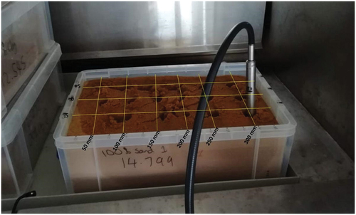
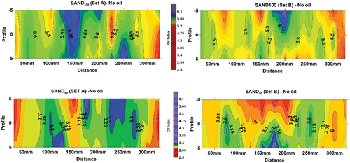
Four ‘boxed’ samples (two SAND₁₀₀, two SAND₉₀) were prepared to investigate oil penetration in 3D. 8000 mL of each soil was placed in a 9000 mL capacity rectangular plastic boxes. A pre-contamination baseline set of measurements was taken by measuring spectra in a grid pattern on the surface of each boxed sample. It was considered a reasonable assumption that this surface measurement in a well-mixed soil sample will be representative of the spectral response at any depth in the sample prior to treatment (Figure A2).

Two sample boxes (one each of SAND₁₀₀ and SAND₉₀) were contaminated in a dry condition. To each sample box, 500 mL of synthetic crude oil was added by slowly pouring it from a measuring cylinder held just above the sample surface in the center of the box. The other two sample boxes were contaminated in a moistened state. Prior to adding 500 mL of oil as above, 250 mL of deionized water was added to this set of boxed samples. This was done using a spray bottle to minimize sample disturbance.

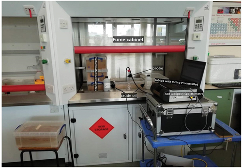
After the addition of oil to all four boxes, they were left undisturbed for 7 days to allow natural infiltration and spatial movement to occur. Throughout this process, all samples were stored in a vertical laminar fume cabinet (Figure A3) to ensure no harmful emissions accumulated.

After 7 days, each sample was subject to 3D spectral probing. All measurements were again carried out in a fume cabinet for purposes of safety. Measurements were captured using the same ASD Labspec4 with an 18 mm steel chamber probe. This probe enables the capture of spectra through a sealed, optically clear window at the base of the probe. The window is mounted at 45° to the probe body, which enables it to be pushed into the sample. Spectral scanning was carried out on a grid with a 50 mm lateral spacing (Figure A4). It was established by initial testing that this resulted in little disturbance to adjoining measurement points. At each grid coordinate, the probe was pushed vertically into the soil to depths of −25 mm, −50 mm, −75 mm, and −100 mm and readings were taken at each depth. It was ensured that after each set of measurements, the probe was thoroughly cleaned to minimize cross-contamination at the next sampling point.

Because the study was about a proof of concept for mapping oil contamination on the subsurface and estimating relative concentrations within a set of samples, replicas were not used. However, an in-depth investigation is ongoing on the real-time monitoring of oil contaminant in different soil types.

2.4 Data analysis

Data were analyzed using Microsoft Excel and Golden Software Surfer 13 version. To compare sample homogeneity of each soil mixtures, reflectance values at 1400 nm; which characterize the uncontaminated soil (accords with Zhao et al. (2018)). Values at this wavelength were converted to grid files in Surfer 13 and surface maps produced. 1720 nm was considered a reasonable wavelength to indicate the presence of oil in soils. Due to the difference in albedo between the dry and wet soil samples, which was observed to affect the oil peak intensities, it was reasonable to compare peak ratios in different regions of the spectrum. A ratio between the oil-reactive wavelength at 1720 nm and a relatively unreactive part of the spectrum, chosen to be 450 nm, was created. The resultant ratio is termed here the “Oil Index” (O_ix) (equation 1(1) $(O_{ix}=\frac{{\lambda }_{n1720}}{{\lambda }_{450}})$(1) ). This was used for baseline measurements; to characterize contaminated vs uncontaminated samples and to estimate relative oil concentrations.

(1) $(O_{ix}=\frac{{\lambda }_{n1720}}{{\lambda }_{450}})$(1)

3. Results

3.1 Spectral signatures

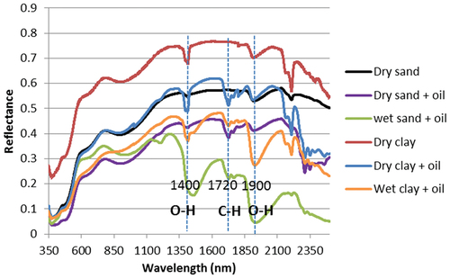
The spectra of oil, water, and soil substrates (uncontaminated and contaminated) are shown in Figure 1. They are distinguished mainly by the spectral geometry between 1300 nm and 2300 nm. The characteristic absorption peak at 1720 nm was indicative of crude oil content. This agrees with (Clark et al. 1990) and others who have found good relationships in that region. For instance, 1716 nm (Douglas et al. 2019); 1712 nm (Okparanma, Coulon, and Mouazen 2014); 1725 nm (Antonov et al. 1999; Chakraborty et al. 2010; Ma et al. 2019; McDowell et al. 2012; Scafutto and Souza Filho 2016). It is relevant to note that broad absorption peaks around 1400 nm – 1450 nm and between 1850 nm – 2100 nm are often related to the presence of water (Douglas et al. 2019; Wartini, Malone, and Minasny 2017; Okparanma, Coulon, and Mouazen 2014; Okparanma and Mouazen 2013a), while a sharp peak at 1400 nm relates to clay (Hermansen et al. 2016; Nawar et al. 2016; Scafutto and Souza Filho 2016; Viscarra Rossel et al. 2006; Wartini, Malone, and Minasny 2017; Zhao et al. 2018).

Figure 1. Distinctive spectra of various mixtures of sand, clay, water and oil. Absorption peak at 1720 nm distinguishes oil-contaminated vs uncontaminated soil samples. Spectral signatures with broad peaks around 1400 nm and 1900 nm are indicative of water, while sharp peaks at 1400 nm characterize soil samples.

3.2 Calibration plots

Plots of spectra and regression curves of reflectance/Oil Index vs oil content (Figure 2) show inverse relationships in all the dry mixtures, with Coefficient of Determination (R²) values of 0.99. Although there was a decrease in Oil Index values with increasing moisture and clay content (compare Figures 2 c vs d), the inverse relationship remains the same for the wet soil mixtures. Oil Index values ranged from approximately 9 at 5% oil to 2.1 at 30% oil content for the SAND₁₀₀, while 7.9 and 1.55 were recorded at 5% and 30% in SAND₉₀.

Figure 2. (a) Calibration plot showing inverse relationship between Oil Index vs oil content for dry SAND₁₀₀. (b) calibration plot for dry SAND₉₀. (c) A polynomial regression plot of Oil Index vs oil content in dry SAND₁₀₀ showing good correlation. (d) A plot showing good correlation for Oil Index vs oil content in SAND₉₀ (e) A good correlation for Oil Index vs oil content in wet SAND₁₀₀ (f) A plot showing poor correlation for Oil Index vs oil content in SAND₉₀.

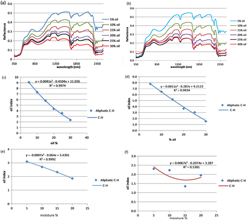
In the wet calibration experiment, only SAND₁₀₀ showed a good correlation between Oil Index and increasing moisture content by up to 20%. R² value of 0.99 was obtained. This indicates a good instrument sensitivity at higher fluid content in sand. In the SAND₉₀ sample, however, a poor relationship was obtained (Figure 2f). This was envisaged to be due to the dilatancy effect of the clay-rich mixture on the probe sensitivity rather than the spectral response of the contaminant. This phenomenon is being investigated in an ongoing study.

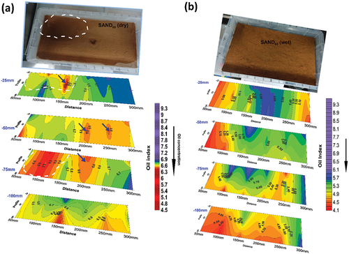
3.3. 3D oil monitoring in SAND₁₀₀

Sub-surface probing of the contaminated soils was carried out at −25 mm intervals, to a maximum depth of −100 mm along three profile lines, allowing for the production of slice-maps. Each slice represents equal depth. The spatial distribution of oil contaminant for SAND₁₀₀ is shown in the picture in Figure 3a, with the 3D delineated feature from spectral data in the slice-map directly beneath the picture. Areas with high oil concentration are characterized by Oil Index values of 6.5 to 8.0, while areas with values of 8.50 and above have low oil. The limited lateral movement of the oil in SAND₁₀₀ was associated with the high porosity of the sample where vertical infiltration was dominant, hence the broad funnel-shaped feature delineated by the white dotted line on the slice-maps.

Figure 3. (a) Slice-map showing a 3D outline of oil contaminant plume in SAND₁₀₀, delineated area (white dotted line). Average Oil Index = 7.7. (b)Slice-map of wet SAND₁₀₀. Spatial variation along slice surfaces may be due to relative displacement of water and oil. Note the lower index values at the bottom slice, indicating fluid accumulation.

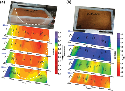
In the wet mixture, Oil Index values were variable due to moisture content. From 6.4 at the bottom to 8.9 at the top. This pattern was expected. The higher spectral values (low oil concentration) at the top layers indicate the nature of movement of the two fluids (oil and water) in a porous sand medium where they moved quickly and accumulated at the bottom due to higher porosity and poor oil-retention of sand. This corroborates the observed scenario in the dry mixture. However, the spatial variation along individual slices was envisaged to be due to the relative displacement of oil and water, a scenario that was not observed in the dry SAND₁₀₀. As depicted in the slice-maps, greater variability of Oil Index values occurs along each slice compared to dry SAND₁₀₀. For instance, at −70 mm depth (third slice), Oil Index values around the central part differ greatly. Values from 7.25 to 7.50 and up to 8 were recorded, although visually, the oil appeared to be uniformly distributed.

3.4. 3D oil monitoring in SAND₉₀

In dry SAND₉₀, oil was observed to spread more laterally compared to dry SAND₁₀₀. Visual observation during the experiment showed a pool of oil formed around the top-left corner of the box (white oval dotted line) due to a slight dip on the mixture’s surface (Figure 4a top picture). This feature has also been delineated on the slice map. The area with the highest oil concentration (Oil Index <6.0) occurs at the left corner of the map at −75 mm (third slice). This coincides with the area where the oil pool formed during oil dosing. Outside this area, Oil Index values range from 6.5 to 6.7 throughout the contaminated soil mixture. The similarity in index values suggests a uniform distribution of the oil contaminant across the entire mixture compared to the SAND₁₀₀ where lower values were restricted to the central part and increased outward toward the edges at both ends. Small pockets of low Oil Index (about 6.3) found in discrete areas (e.g. around 150 mm at −25 mm (2nd slice), and around 250 mm at −50 mm (3rd slice)) in SAND₉₀ were attributed to possible preferential movement and accumulation of oil through minor fissures in the soil.

Figure 4. (a) Slice-map of dry SAND₉₀ sand showing the spatial distribution of oil in the subsurface. The white dotted lines on the first and third slice delineate oil pool formed on the surface in the picture above. Average Oil Index = 6.6. Blue arrows indicate possible oil accumulation in minor fissures. (b) Slice-map of wet SAND₉₀ soil showing spatial distribution of oil (and water). Note the reduced Oil Index values and accumulated fluids toward the bottom.

In wet SAND₉₀, it was envisaged that the movement of oil would be influenced by the presence of moisture in the available pore spaces. The Oil Index values were also reduced due to the combined influence of clay and moisture. Values range from 4.4 at the bottom to 5.85 at the top (compare with 6.5 to 6.7 in the dry mixture). In addition, variability of Oil Index values was observed on individual slices, although, minimal compared to wet SAND₁₀₀ (Figure 4b). This phenomenon also suggests relative displacement of oil and water during movement. For instance, at −25 mm (top slice), Oil Index values range from 4.90 at the left corner to 5.6 around the central part and 4.95 at the lower right corner. Similarly, at −50 mm (2nd slice) and −75 mm (3rd slice), Oil Index values vary across the slices and the lowest values (<4.9) at the bottom slice suggest fluid accumulation. This was tested and the result was presented in the next section.

3.5 Relative concentration in soil mixtures

The average concentration of oil in the two dry soil mixtures (SAND₁₀₀, SAND₉₀) after 7 days was compared. Considering the contaminated mixtures, the average Oil Index for SAND₁₀₀ was 7.7 which equals approximately 8.5% oil content (calculated from the line equation of the calibration plot). Similarly, 6.6 was found to be the average Oil Index in SAND₉₀ and equals 8.8% oil. It was anticipated that since equal volume of oil was added to the different soil mixtures and kept under the same condition over time (7 days), they should have similar concentrations. This was found to be the case. Both dry SAND₁₀₀ and SAND₉₀ compare in their average oil concentration (8.5% and 8.8% respectively) over the same period. The slightly higher value in SAND₉₀ was not unexpected, as clay-rich soils have better fluid retention capacity and are less susceptible to fluid escape due to evaporation compared to sands. Although this scenario gives an idea of possible soil/oil interaction, there are no studies published in the literature using NIR technique to compare with the findings in this study.

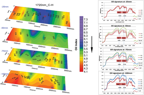
In the wet soil mixtures, estimation of average concentration was less straightforward, especially in SAND₉₀. This was not entirely unexpected as Oil Index was slightly modified by clay and water as reported in the literature (Okparanma and Mouazen 2013a). Since differential movement of oil and water in the soil mixtures could have occurred due to their immiscibility, estimation of oil concentration was done by spectral visualization analysis at selected anomalous points on the slice maps to understand spatial distribution of oil and possible soil/oil interaction.

The spectral plots adjacent to each slice in Figure 5 represent the different points under consideration. Discrimination of different oil vs water was based on characteristic peaks at 1720 nm and ~1400 nm, respectively, while relative oil concentration was determined using the intensity of oil-absorption peaks. Higher oil content would have stronger peaks and vice versa. This approach is similar to the work of (Pabón and de Souza Filho 2016) where oil concentration was related to the “depth” of absorption peaks. On the top slice (depth = 25 mm), all the points E1, E2, and E3 have absorption peaks of oil and water and differ only in their intensities. On the second slice (depth = 50 mm), spectral geometries of points F1 and F3 (having oil peaks) clearly differ from F2 (no oil peak). Similarly, points G1, G2, and G3 (depth = 75 mm) differ in both spectral geometry and oil peak intensities. Similarly, at the bottom slice (depth = 100 mm), points H1 and H4 show stronger oil absorption peaks compared to H2 and H3. This explains the relative displacement of oil and water during their movements from top to bottom of the sample.

Figure 5. Slice map of wet SAND₉₀ mixture showing points where spectral visualization were done at various depths. Oil peak occur at 1720 nm. Brown spectra (F1, F3, G2, H1, H4) are indicative of relatively high oil concentration, blue spectra (G3, H2, H3) indicate low concentration while green spectra (F2, G1) show areas where water preferentially accumulated relative to oil.

4. Discussion

The findings in this study corroborate the reported inverse relationship between reflectance and oil concentration (Douglas et al. 2018; Okparanma and Mouazen 2013b; Pabón and de Souza Filho 2016; Scafutto and Souza Filho 2016; Wartini, Malone, and Minasny 2017). Empirical calibration using known oil concentrations also serves as a simple model for the validation and elimination of errors (e.g. Pabón and de Souza Filho 2016). In addition, the Oil Index derived from peak ratios in this study proved useful in estimating oil concentration. This accords with similar approaches in the literature (e.g. Forrester et al. 2013; Hannisdal, Hemmingsen, and Sjöblom 2005; Klavarioti et al. 2014; Okparanma and Mouazen 2013a). In a recent work, Scafutto and de Souza Filho (2019) calculated peak ratios of hydrocarbon signatures in the NIR region and applied them to discriminate different hydrocarbon types in oil-contaminated samples. Similarly, peak ratios have been effectively used in remote sensing to estimate oil concentrations. These include Normalized Difference Vegetation Index (NDVI), Normalized Difference Water Index (NDWI) (Adamu, Tansey, and Ogutu 2015; Lassalle et al. 2019; Mena et al. 2017; Ozigis, Kaduk, and Jarvis 2019) and Hydrocarbon Index (HI) (Kühn, Oppermann, and Hörig 2010). The Oil Index used in this study also serves the purpose of estimating oil concentration.

In terms of subsurface investigations, 3D analysis of oil-contaminated soils using NIR Spectroscopy has been sparsely reported in the literature. This may be attributed to the limitations of current probes and the lack of a standard method of investigation. Hence, the approach, in this study provides an empirical method for investigating the spatial distribution of oil contaminants in both dry and wet conditions. Similar to ERT, deduction of spatio-temporal movement of oil and water in the subsurface was done using Oil Index and anomalous patterns were identified on slice maps. Furthermore, the estimation of the average concentration in the different soil samples was significant. The slightly higher volume average in the SAND₉₀ (8.8%) relative to the SAND₁₀₀ (8.5%) agrees with the sorption models where adsorption of oil onto soil particles has been reported to increase with increasing clay content (Nudelman, Rios, and Katusich 2000; Ríos and Nudelman 2005; Wu, He, and Chen 2013). Similarly, the relative displacement of oil and water in wet samples, as described in this study, gives an idea of possible desorption which has been reported to increase with changing temperature and higher moisture content (Wu et al. 2015). This finding can be further explored and developed to enhance the field application of NIR Spectroscopy.

5. Conclusion

The work aimed to demonstrate whether information useful for the understanding of contaminant movement can be determined using NIR spectroscopy and also whether the method developed could be applied as a real-time monitoring protocol in support of effective management plans. The findings show the potential application of NIR spectroscopy for subsurface investigations of oil-contaminated sites in dry and wet conditions. While Oil Index alone proved useful in estimating oil concentration in dry soils, spectral visualization of discrete points was needed in wet soils. Furthermore, the slice-maps which captured the spatial distribution of oil contaminants enabled the estimation of average concentrations and enhanced our understanding of oil movement through different soils. Although there are generic computer models (mainly numeric models) that are used to model the movement of contaminants through the soil profile via pore spaces by complex transport mechanisms (Bear and Cheng 2010), these models, are difficult to adapt taking into account local field conditions. Hence, this study attempts to bridge that gap.

One limitation of depth-probing is the slight substrate disturbance during measurement. Nevertheless, the direct and rapid in-situ investigation and ability to discriminate between different fluids based on their spectral signatures outweigh that limitation. In addition, with improved probe design (i.e., much smaller diameter and higher resolution), insignificant disturbance of the soil will further enhance this technique to achieve rapid in-situ and cost-effective sub-surface investigation in small oil-contaminated fields.

Acknowledgments

The authors appreciate James Coyne for providing technical support.

Disclosure statement

No potential conflict of interest was reported by the author(s).

Additional information

Funding

The authors thank the Petroleum Technology Development Fund (PTDF) Nigeria for sponsoring the research.

Appendix A:

Samples of synthetic crude oil obtained from Breckland Scientific Ltd

Appendix B:

Baseline slice-map at 1720 nm showing similar Oil Index for uncontaminated surfaces of SAND₁₀₀ and SAND₉₀ sets.

Appendix C:

Experiment set up. All measurements and storage of samples were done in a fume cabinet

Appendix D:

Grid of sample points for depth probing.

References

- Adamu, B., K. Tansey, and B. Ogutu. 2015. Using vegetation spectral indices to detect oil pollution in the Niger Delta. Remote Sens. Lett. 6 (2):145–54. doi:10.1080/2150704X.2015.1015656.
- Antonov, L., G. Gergov, V. Petrov, M. Kubista, and J. Nygren. 1999. UV-Vis spectroscopic and chemometric study on the aggregation of ionic dyes in water. Talanta 49 (1):99–106. doi:10.1016/S0039-9140(98)00348-8.
- Aske, N., H. Kallevik, and J. Sjöblom. 2001. Determination of saturate, aromatic, resin, and asphaltenic (SARA) components in crude oils by means of infrared and near-infrared spectroscopy. Energy Fuels 15 (5):1304–12. doi:10.1021/ef010088h.
- Bear, J., and A. H.-D. Cheng. 2010. Modeling groundwater flow and contaminant transport, 1st ed. Springer Netherlands. doi:10.1007/978-1-4020-6682-5.
- Brown, S. R., D. Lesmes, J. Fourkas, and J. R. Sorenson. 2003. Complex electrical resistivity for monitoring DNAPL contamination. 29.
- Buzmakov, S., D. Egorova, and E. Gatina. 2019. Effects of crude oil contamination on soils of the Ural region. J. Soils. Sediments 19 (1):38–48. doi:10.1007/s11368-018-2025-0.
- Cassiani, G., A. Binley, A. Kemna, M. Wehrer, A. F. Orozco, R. Deiana, J. Boaga, M. Rossi, P. Dietrich, U. Werban, et al. 2014. Noninvasive characterization of the Trecate (Italy) crude-oil contaminated site: Links between contamination and geophysical signals. Environ Sci. Pollut. Res. 21 (15):8914–31. doi:10.1007/s11356-014-2494-7.
- Chakraborty, S., D. C. Weindorf, C. L. S. Morgan, Y. Ge, J. M. Galbraith, B. Li, and C. S. Kahlon. 2010. Rapid identification of oil-contaminated soils using visible near-infrared diffuse reflectance spectroscopy. J. Environ. Qual. 39 (4):1378–87. doi:10.2134/jeq2010.0183.
- Chakraborty, S., D. C. Weindorf, B. Li, A. A. Ali Aldabaa, R. K. Ghosh, S. Paul, and M. Nasim Ali. 2015. Development of a hybrid proximal sensing method for rapid identification of petroleum contaminated soils. Sci. Total Environ. 514:399–408. doi:10.1016/j.scitotenv.2015.01.087.
- Clark, R. N., T. V. V. King, M. Klejwa, G. A. Swayze, and N. Vergo. 1990. High spectral resolution reflectance spectroscopy of minerals. J. Geophys. Res. Solid Earth 95 (B8):12653–80. doi:10.1029/JB095iB08p12653.
- Coria, D., V. Bongiovanni, N. Bonomo, M. De La Vega, and M. T. Garea. 2009. Hydrocarbon contaminated soil: Geophysical-chemical methods for designing remediation strategies. Near Surf. Geophys. 7 (3):227–36. doi:10.3997/1873-0604.2009020.
- Delgado-Rodríguez, O., V. Shevnin, J. Ochoa-Valdés, and A. Ryjov. 2006a. Geoelectrical characterization of a site with hydrocarbon contamination caused by pipeline leakage. Geofis. Int. 45 (1):63–72. doi:10.22201/igeof.00167169p.2006.45.1.192.
- Delgado-Rodríguez, O., V. Shevnin, J. Ochoa-Valdés, and A. Ryjov. 2006b. Using electrical techniques for planning the remediation process in a hydrocarbon contaminated site. Rev. Int. Contam. Ambient 22 (4):157–63.
- Delgado-Rodríguez, O., D. Flores-Hernández, M. A. Amezcua-Allieri, V. Shevnin, A. Rosas-Molina, and S. Marin-Córdova. 2014. Joint interpretation of geoelectrical and volatile organic compounds data: A case study in a hydrocarbons contaminated urban site. Geofis. Int. 53 (2):183–98. doi:10.1016/s0016-7169(14)71499-0.
- Douglas, R. K., S. Nawar, S. Cipullo, M. C. Alamar, F. Coulon, and A. M. Mouazen. 2018. Evaluation of vis-NIR reflectance spectroscopy sensitivity to weathering for enhanced assessment of oil contaminated soils. Sci. Total Environ. 626:1108–20. doi:10.1016/j.scitotenv.2018.01.122.
- Douglas, R. K., S. Nawar, M. C. Alamar, F. Coulon, and A. M. Mouazen. 2019. Rapid detection of alkanes and polycyclic aromatic hydrocarbons in oil-contaminated soil with visible near-infrared spectroscopy. Eur. J. Soil Sci. 70 (1):140–50. doi:10.1111/ejss.12567.
- Forrester, S. T., L. J. Janik, M. J. McLaughlin, J. M. Soriano-Disla, R. Stewart, and B. Dearman. 2013. Total petroleum hydrocarbon concentration prediction in soils using diffuse reflectance infrared spectroscopy. Soil Sci. Soc. Am. J. 77 (2):450–60. doi:10.2136/sssaj2012.0201.
- Ghandehari, M., K. Kostarelos, K.-C. Cheng, C. Vimer, and S. Yoon. 2008. Near-infrared spectroscopy for in situ monitoring of geoenvironment. J. Geotech. Geoenviron. Eng. 134 (4):487–96. doi:10.1061/(ASCE)1090-0241(2008)134:4(487).
- Hannisdal, A., P. V. Hemmingsen, and J. Sjöblom. 2005. Group-type analysis of heavy crude oils using vibrational spectroscopy in combination with multivariate analysis. Ind. Eng. Chem. Res. 44 (5):1349–57. doi:10.1021/ie0401354.
- Hermansen, C., M. Knadel, P. Moldrup, M. H. Greve, R. Gislum, and L. W. de Jonge. 2016. Visible-near-infrared spectroscopy can predict the clay/organic carbon and mineral fines/organic carbon ratios. Soil Sci. Soc. Am. J. 80 (6):1486–95. doi:10.2136/sssaj2016.05.0159.
- Ioane, D., P. Georgescu, F. Chitea, A. Diaconu, B. M. Niculescu, and M. Mezincescu (1999). Geophysical detection and monitoring of underground pollution with hydrocarbon contaminants. 4000.
- Klavarioti, M., K. Kostarelos, A. Pourjabbar, and M. Ghandehari. 2014. In situ sensing of subsurface contamination-part I: Near-infrared spectral characterization of alkanes, aromatics, and chlorinated hydrocarbons. Environ Sci. Pollut. Res. 21 (9):5849–60. doi:10.1007/s11356-013-2478-z.
- Kühn, F., K. Oppermann, and B. Hörig. 2010. Hydrocarbon Index – An algorithm for hyperspectral detection of hydrocarbons. 1161. Taylor & Francis Group. doi: 10.1080/01431160310001642287.
- Lassalle, G., A. Elger, A. Credoz, R. H’dacq, G. Bertoni, D. Dubucq, and S. Fabre. 2019. Toward quantifying oil contamination in vegetated areas using very high spatial and spectral resolution imagery. Remote Sens. 11 (19):2241. doi:10.3390/rs11192241.
- Ma, L., Y. Peng, Y. Pei, J. Zeng, H. Shen, J. Cao, Y. Qiao, and Z. Wu. 2019. Systematic discovery about NIR spectral assignment from chemical structural property to natural chemical compounds. Sci. Rep. 9 (1):1–17. doi:10.1038/s41598-019-45945-y.
- Malley, D. F., K. N. Hunter, and G. R. B. Webster. 1999. Analysis of diesel fuel contamination in soils by near-infrared reflectance spectrometry and solid phase microextraction-gas chromatography. Oil Sediment Contam. 8 (4):481–89. doi:10.1080/10588339991339423.
- McDowell, M. L., G. L. Bruland, J. L. Deenik, S. Grunwald, and N. M. Knox. 2012. Soil total carbon analysis in Hawaiian soils with visible, near-infrared and mid-infrared diffuse reflectance spectroscopy. Geoderma 189– 190:312–20. doi:10.1016/j.geoderma.2012.06.009.
- Mena, C. F., C. Sampedro, P. E. Martinez, H. Paltan, A. Encarnación, and D. Zambrano. 2017. Remote sensing of oil spills: Linking community monitoring and satellite image processing in the Ecuadorian Amazon. Comp Remote Sens. 1– 9:144–58. doi:10.1016/B978-0-12-409548-9.10425-7.
- Mendelssohn, I. A., G. L. Andersen, D. M. Baltz, R. H. Caffey, K. R. Carman, J. W. Fleeger, S. B. Joye, Q. Lin, E. Maltby, E. B. Overton, et al. 2012. Oil impacts on coastal wetlands: Implications for the Mississippi River delta ecosystem after the deepwater horizon oil spill. BioScience 62 (6):562–74. doi:10.1525/bio.2012.62.6.7.
- Morgan, C. L. S., T. H. Waiser, D. J. Brown, and C. T. Hallmark. 2009. Simulated in situ characterization of soil organic and inorganic carbon with visible near-infrared diffuse reflectance spectroscopy. Geoderma 151 (3–4):249–56. doi:10.1016/j.geoderma.2009.04.010.
- Mullins, O. C., S. Mitra-Kirtley, and Y. Zhu. 1992. The electronic absorption edge of petroleum. Appl. Spectrosc. 46 (9):1405–11. doi:10.1366/0003702924123737.
- Nawar, S., H. Buddenbaum, J. Hill, J. Kozak, and A. M. Mouazen. 2016. Estimating the soil clay content and organic matter by means of different calibration methods of vis-NIR diffuse reflectance spectroscopy. Soil Till. Res. 155:510–22. doi:10.1016/j.still.2015.07.021.
- Nudelman, N. S., S. M. Rios, and O. Katusich. 2000. Interactions between crude oil and Patagonian soil as a function of the soil clay-water content. Environ. Technol. (UK) 21 (4):437–45. doi:10.1080/09593332108618105.
- Okparanma, R. N., and A. M. Mouazen. 2013. Determination of total petroleum hydrocarbon (TPH) and polycyclic aromatic hydrocarbon (PAH) in soils: A review of spectroscopic and nonspectroscopic techniques. Appl. Spectrosc. Rev. 48 (6):458–86. doi:10.1080/05704928.2012.736048.
- Okparanma, R. N., and A. M. Mouazen. 2013a. Combined effects of oil concentration, clay and moisture contents on diffuse reflectance spectra of diesel-contaminated soils. Water Air Soil Pollut. 224 (5). doi: 10.1007/s11270-013-1539-8.
- Okparanma, R. N., and A. M. Mouazen. 2013b. Visible and near-infrared spectroscopy analysis of a polycyclic aromatic hydrocarbon in soils. Sci. World J. 2013:1–9. doi:10.1155/2013/160360.
- Okparanma, R. N., F. Coulon, and A. M. Mouazen. 2014. Analysis of petroleum-contaminated soils by diffuse reflectance spectroscopy and sequential ultrasonic solvent extraction-gas chromatography. Environ. Pollut. 184:298–305. doi:10.1016/j.envpol.2013.08.039.
- Okparanma, R. N., F. Coulon, T. Mayr, and A. M. Mouazen. 2014. Mapping polycyclic aromatic hydrocarbon and total toxicity equivalent soil concentrations by visible and near-infrared spectroscopy. Environ. Pollut. 192:162–70. doi:10.1016/j.envpol.2014.05.022.
- Ozigis, M. S., J. D. Kaduk, and C. H. Jarvis. 2019. Mapping terrestrial oil spill impact using machine learning random forest and Landsat 8 OLI imagery: A case site within the Niger Delta region of Nigeria. Environ Sci. Pollut. Res. 26 (4):3621–35. doi:10.1007/s11356-018-3824-y.
- Pabón, R. E. C., and C. R. de Souza Filho. 2016. Spectroscopic characterization of red latosols contaminated by petroleum-hydrocarbon and empirical model to estimate pollutant content and type. Remote Sens. Environ. 175:323–36. doi:10.1016/j.rse.2016.01.005.
- Pabón, R. E. C., C. R. de Souza Filho, and W. J. de Oliveira. 2019. Reflectance and imaging spectroscopy applied to detection of petroleum hydrocarbon pollution in bare soils. Sci. Total Environ. 649. doi:10.1016/j.scitotenv.2018.08.231.
- Ríos, S. M., and N. S. Nudelman. 2005. Multilayer sorption model for the interactions between crude oil and clay in Patagonian soils. J. Dispers. Sci. Technol. 26 (1):19–25. doi:10.1081/DIS-200040228.
- Scafutto, R. D. M., and C. R. D. Souza Filho. 2016. Quantitative characterization of crude oils and fuels in mineral substrates using reflectance spectroscopy: Implications for remote sensing. Int. J. Appl. Earth Obs. Geoinf. 50:221–42. doi:10.1016/j.jag.2016.03.017.
- Scafutto, R. D. M., and C. R. de Souza Filho. 2019. Detection of heavy hydrocarbon plumes (Ethane, propane and Butane) using airborne long wave (7.6–13.5 μm) infrared hyperspectral data. Fuel 242:863–70. doi:10.1016/j.fuel.2018.12.127.
- Shevnin, V., O. Delgado-Rodríguez, A. Mousatov, E. Nakamura-Labastida, and A. Mejía-Aguilar. 2003. Oil pollution detection using resistivity sounding. Geofis. Int. 42 (4):613–22. doi:10.22201/igeof.00167169p.2003.42.4.315.
- Townsend, G. T., R. C. Prince, and J. M. Suflita. 2003. Anaerobic oxidation of crude oil hydrocarbons by the resident microorganisms of a contaminated anoxic aquifer. Environ. Sci. Technol. 37 (22):5213–18. doi:10.1021/es0264495.
- Viscarra Rossel, R. A., D. J. J. Walvoort, A. B. McBratney, L. J. Janik, and J. O. Skjemstad. 2006. Visible, near infrared, mid infrared or combined diffuse reflectance spectroscopy for simultaneous assessment of various soil properties. Geoderma 131 (1–2):59–75. doi:10.1016/j.geoderma.2005.03.007.
- Wang, X., J. Feng, and J. Zhao. 2010. Effects of crude oil residuals on soil chemical properties in oil sites, Momoge Wetland, China. Environ. Monit. Assess. 161 (1–4):271–80. doi:10.1007/s10661-008-0744-1.
- Wang, Y., J. Feng, Q. Lin, X. Lyu, X. Wang, and G. Wang. 2013. Effects of crude oil contamination on soil physical and chemical properties in momoge wetland of China. Chin. Geogr. Sci. 23 (6):708–15. doi:10.1007/s11769-013-0641-6.
- Wartini, N., B. P. Malone, and B. Minasny. 2017. Rapid assessment of petroleum-contaminated soils with infrared spectroscopy. Geoderma 289:150–60. doi:10.1016/j.geoderma.2016.11.030.
- Wu, G., L. He, and D. Chen. 2013. Sorption and distribution of asphaltene, resin, aromatic and saturate fractions of heavy crude oil on quartz surface: Molecular dynamic simulation. Chemosphere 92 (11):1465–71. doi:10.1016/j.chemosphere.2013.03.057.
- Wu, G., X. Zhu, H. Ji, and D. Chen. 2015. Molecular modeling of interactions between heavy crude oil and the soil organic matter coated quartz surface. Chemosphere 119:242–49. doi:10.1016/j.chemosphere.2014.06.030.
- Zhao, D., X. Zhao, T. Khongnawang, M. Arshad, and J. Triantafilis. 2018. A Vis-NIR spectral library to predict clay in Australian cotton growing soil. Soil Sci. Soc. Am. J. 82 (6):1347–57. doi:10.2136/sssaj2018.03.0100.