Comparison of remote sensing indices for monitoring of desert cienegas

ABSTRACT

This research considers the applicability of different vegetation indices at 30 m resolution for mapping and monitoring desert wetland (cienega) health and spatial extent through time at Cienega Creek in southeastern Arizona, USA. Multiple stressors including the risk of decadal-scale drought, the effects of current and predicted global warming, and continued anthropogenic pressures threaten aquatic habitats in the southwest and cienegas are recognized as important sites for conservation and restoration efforts. However, cienegas present a challenge to satellite-imagery based analysis due to their small size and mixed surface cover of open water, exposed soils, and vegetation. We created time series of five well-known vegetation indices using annual Landsat Thematic Mapper (TM) images retrieved during the April–June dry season, from 1984 to 2011 to map landscape-level distribution of wetlands and monitor the temporal dynamics of individual sites. Indices included the Normalized Difference Vegetation Index (NDVI), the Soil-Adjusted Vegetation Index (SAVI), the Normalized Difference Water Index (NDWI), and the Normalized Difference Infrared Index (NDII). One topographic index, the Topographic Wetness Index (TWI), was analyzed to examine the utility of topography in mapping distribution of cienegas. Our results indicate that the NDII, calculated using Landsat TM band 5, outperforms the other indices at differentiating cienegas from riparian and upland sites, and was the best means to analyze change. As such, it offers a critical baseline for future studies that seek to extend the analysis of cienegas to other regions and time scales, and has broader applicability to the remote sensing of wetland features in arid landscapes.

KEYWORDS:

• Landsat
• normalized difference infrared index
• normalized difference vegetation index
• semiarid grasslands
• wetlands

Introduction

Cienegas

Cienegas (Spanish for “swamp” or “marsh”) are low- to mid-elevation, slow-flowing, perennial wetlands that are found in arid landscapes of the U.S. southwest. Cienegas are a minor areal component of riparian systems in the region but they exert a disproportionately significant ecological influence. The presence of riparian and cienega vegetation in an otherwise arid landscape can increase overall biodiversity of a region by 50% (Sabo et al. 2005) and cienegas are recognized as hosting regionally rare and unique plant communities (Caves et al. 2013). Cienegas also provide a number of critical hydrologic services: they regulate downstream flow regimes and indicate the presence of near-surface water availability and landscape-level hydrologic condition (Hendrickson and Minckley 1984; Minckley, Brunelle, and Turner 2013). Cienegas are often found associated with high quality grasslands (Minckley, Turner, and Weinstein 2013) and represent a stable state in nondegraded semi-arid grassland ecological transition models (Minckley, Brunelle, and Turner 2013). Given their ecological functions, measurements of cienega health can provide information on larger landscape processes such as degradation and recovery. As sources of perennial water, these sites were historically heavily utilized by humans in southeast Arizona, primarily for livestock grazing starting in the mid-nineteenth century and subsequently for crop irrigation. This intense anthropogenic utilization is implicated in the degradation of cienegas and their surrounding grassland habitats (Hendrickson and Minckley 1984), though early twentieth century climate change may also have contributed to periods of incision and arroyo-cutting (Waters and Haynes 2001). This trend has continued in recent times with 20% of cienegas experiencing severe degradation since the 1980s (Minckley, Turner, and Weinstein 2013). Given multiple stressors including the risk of decadal scale drought (Ault et al. 2014), the effects of current and predicted global warming (Seager et al. 2007; Dominguez, Cañon, and Valdes 2009; Cayan et al. 2010; Perry et al. 2012), and continued anthropogenic pressures threatening aquatic habitats in the U.S. southwest (Grimm et al. 1997; Villarreal et al. 2013), cienegas are recognized as important sites for conservation and restoration efforts.

Remote sensing data

Multi-temporal remote sensing data offer the ability to map landscape-level distribution of wetlands and monitor the temporal dynamics of individual sites (Ozesmi and Bauer 2002; Kerr and Ostrovsky 2003; Yang 2007; Adam, Mutanga, and Rugege 2010). In southeast Arizona, remote sensing data has been used to evaluate the effects of restoration on riparian habitats (Norman et al. 2014) and to map changes in riparian vegetation (Jones et al. 2008; Villarreal, Leeuwen, and Romo-Leon 2012; Nguyen et al. 2015). In the Sahara-Sahel region of Africa, satellite imagery has been used to identify permanent and temporary sources of water (Campos, Sillero, and Brito 2012), to distinguish artificial from natural sources of water (Owen, Duncan, and Pettorelli 2015), and to monitor water levels in ponds (Soti et al. 2009). These studies relied on a variety of remote sensing data sources (Landsat Thematic Mapper, Moderate Resolution Imaging Spectrometer, and Quickbird) with a variety of temporal and spatial resolutions to analyze different aspects of wetland habitats. Wetland habitats present a challenge to map and monitor using midresolution (30–250 m), multispectral imagery because of their small size, predominately linear, irregular shapes, and mixed composition of land cover types (A; Figure 1). However, mid-resolution imagery such as the Landsat series is attractive due to the time span of collected data (1972–present); no publically available high resolution imagery spans the same breadth of time. Other methods have been used to assess changes in cienegas over the last 7,000 years providing valuable information on cienega formation and ecological succession (Minckley and Brunelle 2007) but they do not provide insight into the effectiveness of management actions performed on a decadal scale. The availability of appropriate time series data, if effective analysis methods are developed, is a key resource in ecological monitoring and land management (Magurran et al. 2010). In the absence of historical field data, remote sensing is invaluable for conservation applications such as monitoring trends in landscape degradation and recovery (Kerr and Ostrovsky 2003).

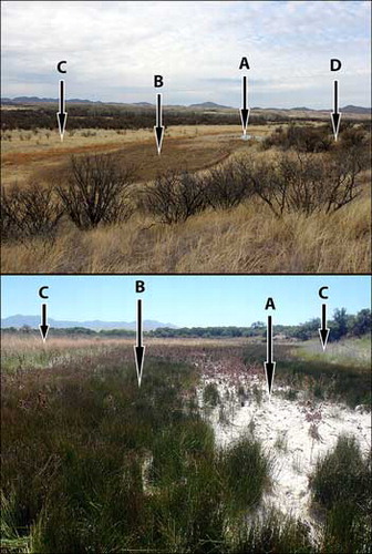
Figure 1. Photos of cienegas at Las Cienegas National Conservation Area (NCA). Top: Cienegas showing a patch of (a) open water with (b) darker, dormant and senescent cienega vegetation surrounded by (c) floodplain grassland and (d) upland shrub savanna/shrubland during the winter rainy season when most vegetation, cienega or other, is senescent. Photo by Andrew Salywon, 2/2/2014. Bottom: A cienega showing (a) white, dried algae cover; (b) dark green cienega vegetation; and (c) light green and brown surrounding vegetation during the dry summer season. The cienega vegetation has greater access to water and shows a stronger greening response than other vegetation before the monsoon season. Photo by Natalie R. Wilson, 6/8/2014.

Over forty different spectral indices have been identified for use in ecological applications (Bannari et al. 1995) and many may be applicable to cienegas. Different remote sensing indices balance sensitivity to environmental elements such as vegetation, open water, and bare soil using a variety of spectral bands (Bannari et al. 1995; Table 1). The Normalized Difference Vegetation Index (NDVI; Rouse et al. 1974), the classic measure of vegetation greenness, was one of the first vegetation indices developed for satellite imagery analysis and is widely used because it strongly correlates with photosynthesis and primary production of vegetation. In the arid U.S. southwest NDVI has been found to correlate with percent cover of riparian vegetation (Nagler, Glenn, and Huete 2001). However, the seasonally-varied amounts of vegetation cover and open water complicate the use of NDVI for characterization of cienegas. NDVI may not be a reliable indicator of green vegetation in cienegas outside of the growing season due to senescent brown vegetation and background soil reflectance in areas of sparse vegetation cover (Huete, Jackson, and Post 1985; Huete and Jackson 1987; Beck, Hutchinson, and Zauderer 1990). To address the influence of soil reflectance in arid regions with low to moderate vegetation cover, Huete (1988) modified the NDVI to create the Soil-Adjusted Vegetation Index (SAVI), which includes a correction factor for soil brightness (L). Cienegas often have areas of open water, which have the effect of lowering NDVI values when intermixed with green vegetation (Justice et al. 1985). The Normalized Difference Water Index (NDWI; McFeeters 1996) was developed to delineate open water features and separate these features from vegetation and soils and may be useful in separating cienegas from the arid surroundings. Two combinations of NIR and short wave infrared (SWIR) bands are possible using Landsat TM data, and the normalized ratios have been used to monitor vegetation water content (Ji et al. 2011). The Normalized Difference Infrared Index using SWIR at 1.65 µm (NDII5) was first developed to measure biomass in salt marsh habitats (Hardisky, Klemas, and Smart 1983), which share characteristics with cienegas such as higher relative soil salinity, increased access to water compared to upland habitats, the presence of standing water, and distinctive vegetation communities. NDII5 correlates with vegetation water content (Jackson et al. 2004), is less attenuated by brown biomass than NDVI (Hardisky et al. 1984), and has been shown to perform well in the identification and monitoring of temporary and permanent water sources in semi-arid lands in Africa (Soti et al. 2009; Campos, Sillero, and Brito 2012). This combination of bands has been identified multiple ways in the literature. It is referred to as the Normalized Difference Water Index when the index developed by Gao (1996) using Moderate-Resolution Imaging Spectroradiometer data is applied to Landsat data (Campos, Sillero, and Brito 2012). More recently it has been referred to as the Normalized Difference Moisture Index (E. H. Wilson and Sader 2002). The Normalized Difference Infrared Index using SWIR at 2.22 µm (NDII7; Chuvieco et al. 2002) has been used to evaluate vegetation cover primarily in the context of wildfire burn severity (García and Caselles 1991) but also in the monitoring of vegetation water content and fuels (Stow, Niphadkar, and Kaiser 2006). In addition to spectral data, topographic data may also be useful in identifying cienegas based on the influence of topography on cienega formation and persistence given the requirement for saturated soils that typically occur in areas with low slope within valley bottoms (Hendrickson and Minckley 1984). The Topographic Wetness Index (TWI), which quantifies soil moisture conditions (Beven and Kirkby 1979), has been correlated with vegetation species composition (Moeslund et al. 2013) and used to predict riparian habitat distribution (Shoutis, Patten, and McGlynn 2010).

Table 1. Summary of indices including both spectral and topographic indices.

Spectral Indices
Index Name	Property Measured	General Formula	Landsat TM Formula
Normalized Difference Vegetation Index (NDVI)	Vegetation Greenness
Soil-Adjusted Vegetation Index (SAVI)	Vegetation Greenness
Normalized Difference Water Index (NDWI)	Open Water
Normalized Difference Infrared Index (NDII5)	Vegetation Moisture Content
Normalized Difference Infrared Index (NDII7)	Vegetation Moisture Content
Topographic Index
Index Name	Property Measured	General Formula
Topographic Wetness Index (TWI)	Wetness Potential

Due to their rarity, their utility as indicators of hydrologic function and as areas of high biodiversity, and the threats they are facing, cienegas are important sites in arid landscapes and land management agencies are increasingly interested in their conservation and restoration. Lack of historical data has hindered efforts to understand recent changes in these unique landforms. Applying remote sensing analysis techniques to mid-resolution, multi-spectral imagery such as Landsat can provide information regarding past trends and monitor future trends in instances where land management resources for monitoring are limited, but only if an appropriate index is identified. The objective of this research is to compare remote sensing indices derived from Landsat imagery collected for a period of 28 years (1984–2011) over a representative sample of cienegas in southeast Arizona in order to identify the most effective index for distinguishing cienegas from surrounding riparian and upland areas and for tracking trends in greenness and moisture as proxies for cienega health. To our knowledge, this study is the first to consider the applicability of different vegetation indices at 30 m resolution for mapping and monitoring cienega health and spatial extent through time. As such, it offers a critical baseline for future studies that seek to extend the analysis of cienegas to other regions and time scales, and has implications for the broader application of remote sensing techniques to monitor other wetland features in arid landscapes.

Materials and methods

Study area

Cienega Creek, 70 km southeast of Tucson and a tributary of the Santa Cruz River, is classified as an “Outstanding Arizona Water” by the Arizona Department of Environmental Quality due to its ecological importance and the purity of its water (Arizona Department of Environmental Quality 2008). In 2000, the area was made a National Conservation Area (NCA) and is managed by the Bureau of Land Management (U.S. Congress 2000). The upper portion of Cienega Creek has one of the most extensive systems of cienegas, historical and extant, in the region (Hendrickson and Minckley 1984). The extant cienegas extend along an 8 km stretch of Cienega Creek (Figure 2). The vegetation of the cienegas is dominated by herbaceous, generally emergent, species (Hendrickson and Minckley 1984) from the following genera: Juncus L., Scirpus L., Eleocharis R. Br., and Carex L. (Bodner and Simms 2008). From 1984 to 2004, fences were erected to exclude cattle from most of Cienega Creek within the NCA. This exclusion has resulted in a conversion from seep-willow shrubland to cottonwood-willow gallery forest along much of the length of the stream channel (Jeff Simms, personal communication, January 22, 2015). The cienegas in the northern end of the NCA exist within the exclosed area around the creek. Most of the cienegas in the southern half of the study area are not included in the creek exclosure but several have been exclosed since 2013 to protect the cienegas from cattle and bullfrogs (personal observation, June 8, 2014). The cottonwood-willow gallery forest that has developed since the exclosure fence was installed is dominated by Populus fremontii S. Wats. and Salix gooddingii C.R. Ball with frequent occurrences of a variety of other mesic tree and understory shrub species. Seep-willow shrubland continues to exist in patches along the riparian corridor and contributing washes; Baccharis salicifolia (Ruiz & Pav.) Pers. is the dominant species with Ambrosia monogyra (Torr. & A. Gray) Strother & B.G. Baldw. as a major associate. Mesquite bosque is another riparian vegetation community at Las Cienegas NCA and is dominated by tall tree-form mesquite, Prosopis velutina Wooton. Sacaton grassland occurs along the floodplain of Cienega Creek and is dominated by perennial grass Sporobolus wrightii Munro ex Scribn. intermixed with patches of the native forb Anemopsis californica (Nutt.) Hook. & Arn. (Bodner and Simms 2008). The uplands are dominated by semi-desert grassland that is primarily a mixture of native perennial grasses; dominant genera include Aristida L., Bouteloua Lag., and Hillaria Kunth though Eragrostis lehmanniana Nees is an exotic perennial grass spreading through region. The semi-desert grassland is also experiencing shrub encroachment and large areas are converting to shrub savanna and shrubland dominated by fabaceous species, most notably Prosopis velutina, but also Senegalia greggii (A. Gray) Britton & Rose, and Vachellia constricta (Benth.) Seigler & Ebinger (Gori and Schussman 2005).

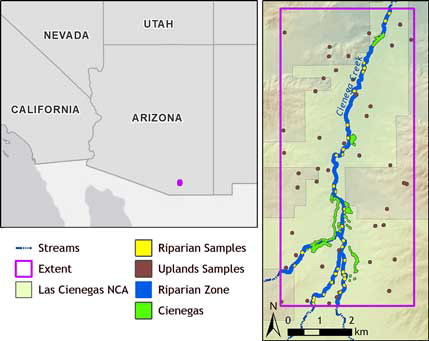
Figure 2. Left: The location of study site in relation to the southwestern USA. Basemaps provided by ESRI et al (2015a, 2015b). Right: The extent of the study area which encompasses 39 km². Cienegas occur along an 8-km length of Cienega Creek. Shown are the cienegas, the riparian habitat zone used to develop the sample groups, and the three sample groups: cienega, riparian, and upland. Cienega, riparian habitat zone, and sample polygons are represented larger than actual size for all areas to be clearly visualized.

Several endangered, threatened and sensitive species occur at Las Cienegas NCA (Caves et al. 2013). The endangered Huachuca water umbel (Lilaeopsis schaffneriana var. recurva (A.W. Hill) Affolter) occurs along the wetted margins of the cienegas (personal observation with Gita Bodner, July 1, 2015) and Cochise sedge (Carex ultra L.H. Bailey), a species of concern in Arizona, is returning to Cienega Creek floodplain (Jeff Simms, personal communication, January 22, 2015). Las Cienegas NCA also supports the best population of the endangered desert fish, Gila topminnow (Poeciliopsis occidentalis (Baird and Girard 1853); Bodner, Simms, and Gori 2007). Current threats to the cienegas of Las Cienegas NCA include climate change, urban and suburban development pressure, mining development, channel erosion, and invasive species (Bodner and Simms 2008). For these reasons, the cienegas of Las Cienegas NCA are important targets for conservation.

Arizona experiences a bimodal precipitation pattern characterized by gentle rains in the winter and monsoons in the late summer. April, May, and June are the driest months of the year and are the months when the presence of water and greenness of vegetation with access to water are typically most distinct from the otherwise dry and senescent landscape; in these dry months cienegas typically have green vegetation due to their higher soil moisture and may have surface water depending on the amount of winter precipitation (Figure 3).

Figure 3. Average monthly precipitation from 1984–2011 at Las Cienegas NCA. The driest months, April, May, and June, directly precede the monsoonal pattern in July and August in which the bulk of annual precipitation occurs. Data acquired May 1, 2014, PRISM Climate Group (Daly et al. 2002).

Remote sensing indices, image selection, and processing

This research, initially explored by N. R. Wilson (2014), focused on five spectral indices: NDVI, SAVI, NDWI, NDII5, and NDII7 (Table 1). NDVI is a measure of greenness, or photosynthetically active vegetation; it is a ratio combination of near infrared (NIR) and visible red spectral bands (Rouse et al. 1974). SAVI is also a ratio combination of NIR and visible red bands but accounts for bare soil reflectance by including an L factor; the coefficient L = 0.5 is suitable for a wide range of vegetation cover and was used for this study (Huete 1988). NDWI is a ratio combination of green and NIR bands (McFeeters 1996). The NDII index is a ratio combination of NIR and SWIR bands; Landsat provides two SWIR bands, both of which were examined in this research. NDII5 uses the SWIR band at 1.65 µm in a ratio combination with NIR (Hardisky, Klemas, and Smart 1983) while NDII7 uses the SWIR band at 2.22 µm with NIR (Chuvieco et al. 2002). One non-spectral index was calculated, the Topographic Wetness Index (TWI) combines upslope flow contributing area (a_s) with slope (β) to quantify soil moisture conditions (Beven and Kirkby 1979).

One Landsat scene was chosen from the seasonal dry months (April–June) for each year from 1984–2011 based on the lack of cloud cover. All scenes were atmospherically corrected using the Modtran 5 atmospheric radiative transfer model and converted to surface reflectance using ATCOR-3 software. Appropriate bands were extracted to calculate the five index values for each scene per year. National Elevation Dataset (NED) digital elevation model (DEM) data at 10 m resolution provided topographic information for the TWI. Landsat and DEM were acquired from the USGS National Map on May 1, 2014 (Dollison 2010).

Sample site selection

To compare the performance of indices in distinguishing cienegas from upland or riparian areas, we developed an experimental design using 121 samples classified by habitat zone within a 39 km² rectangular extent that included all cienegas (Figure 2). The three habitat types compared were cienega, upland, and riparian. The cienega sample consisted of forty four cienegas we located in the field based on the presence of water and relevant vegetation communities in 2013. We recorded the polygonal extent of each cienega with a hand-held GPS; the total land cover encompassed was 154,133 m². Defining upland and riparian areas by vegetation type was difficult due to the temporal extent of the dataset. Since the imagery spans 28 years of land management activities and various land uses there have been conversions in vegetation communities which are difficult to track with precision. Instead, we developed two habitat zones based on proximity to cienegas and the river channel. The upland zone was defined as falling outside a 30 m buffer around all cienegas and stream channels and includes semi-desert grassland, mesquite shrub savanna/shrubland, and sacaton grassland. We chose a random sample of forty-four points from within this zone and buffered each point by 33.4 m to develop a control study area similar in size to the total area of cienegas. A small number of the randomly generated points were close to the boundary of the upland area. When the points were buffered some overlap occurred between the buffered point and the non-upland area; these overlapping areas were excluded resulting in a final upland sample of forty-four polygons covering a total of 151,391 m². The riparian zone was developed by buffering streams and cienegas by 30 m and excluding buffered cienegas. The riparian zone includes cottonwood-willow gallery forest, mesquite bosque, and seep-willow shrubland. Only thirty-three random points could be generated in the riparian zone due to its relatively small extent. These points were also buffered by 33.4 m to maintain consistency between sample groups; any area extending beyond the riparian zone was excluded from the sample, yielding a riparian sample of thirty-three polygons with a total area of 84,542 m².

All spatial data and image processing was conducted in ArcMap 10.2 with the Spatial Analyst extension and ERDAS Imagine using both standard tools and custom scripts developed in python and ERDAS Spatial Modeler Language.

Analysis

Cienegas are small and irregularly shaped, which results in many pixels encompassing a mixture of different land cover types; very few of the TM pixels were purely cienega. The mixed pixels created concern that index comparison methods that rely on excluding some data from the analysis for accuracy testing would have resulted in too few samples for meaningful analysis. Instead, zonal statistics were calculated for each polygon (cienega, riparian, upland) for each index for each year of data. The irregular shape of cienega polygons complicated zonal statistics because polygons were not evenly spread out across TM pixels. To address this issue, index results were resampled to a pixel size of 1 m² prior to the application of zonal statistics for all habitat polygons (cienega, riparian, uplands). This effectively weighted each TM pixel by the area which intersected a polygon for the calculation of zonal statistics. Analysis of Variance (ANOVA; Walford 2011) was applied to the resultant mean values for cienega, riparian, and upland samples to determine if the six indices examined can distinguish between habitat types. An ANOVA analysis of the vegetation cover types for each index, and each year in the case of spectral indices, determines whether the untransformed index values for the different habitats are significantly different. Little of the data approximated a Gaussian curve and no transformation technique normalized the distribution for a large enough subset of the data to warrant a separate analytical process. Untransformed index values were used for the analysis. Levene’s statistic (Levene 1961) was used to assess homogeneity of variances, and Tamhane’s post-hoc analysis, which does not assume homogenous variances (Tamhane 1977), was used to compare between groups. ANOVA and other statistics were calculated in SPSS Statistics.

To analyze temporal trends in the spectral indices of the cienegas, we plotted the five mean index values for each cienega polygon from 1984 to 2011 and applied linear regression to each in SPSS Statistics (Walford 2011). The slope coefficient was used to quantify the trend for individual cienegas. Spatial clustering of trends was examined and associated with land use changes. To explore that possibility, Global Moran’s I (spatial autocorrelation) was calculated in ArcMap 10.2 using Delaunay triangulation (Moran 1948; Zhang and Murayama 2000) for the trends for each spectral index. Global Moran’s I tests for the existence of spatial clustering relative to the null hypothesis of a random distribution.

Results

Analysis of variance

Values of the one measure that incorporated topography (TWI) differed between the cienega, riparian and upland areas as determined by ANOVA (Table 2, F(2,118) = 10.955, P = 0.000). The variances of means were heterogeneous as determined by Levene’s test (P = 0.000) which restricts post hoc testing to methods that do not assume homogenous variances. Tamhane’s post hoc test revealed that mean TWI for cienegas (mean = 625.19, SD = 535.26, P = 0.000) and riparian (mean = 1014.71, SD = 1238.14, P = 0.003) were statistically significantly different than uplands (mean = 226.80, SD = 227.77) but there is no significant difference between cienega and riparian groups (P = 0.266). This indicates that TWI can distinguish upland areas from cienega and riparian areas but cannot distinguish between cienega and riparian areas. TWI values were higher for riparian and cienega than upland cover types. Higher TWI values indicate higher capacity for water accumulation and wetness.

Table 2. Oneway ANOVA and Tamhane’s multiple comparison of mean TWI values for three different habitat types: cienegas, riparian, and upland (P < 0.05).

ANOVA
	Sum of Squares	df	Mean Square	F	Sig.
Between Groups	11809807.612	2	5904903.806	10.955	0.000
Within Groups	63606165.815	118	539035.304
Total	75415973.427	120
Tamhane’s Multiple Comparisons
Type		Mean Difference	Std. Error	Sig.
Cienega	Riparian	–389.526	230.143	0.266
	Upland	398.385	87.695	0.000
Riparian	Cienega	389.526	230.143	0.266
	Upland	787.912	218.251	0.003
Upland	Cienega	–398.385	87.695	0.000
	Riparian	–787.912	218.251	0.003

Interannual variability of climatic factors, such as precipitation and temperature, and their effects on spectral index values could not be accounted for in ANOVA. Mild, wet winters may result in upland areas having similar values to cienega or riparian areas after harsh, dry winters; this would have resulted in an artificially low difference between groups during ANOVA. To avoid this complication, the 28 years of Landsat data were analyzed individually. Five spectral indices were applied to 28 years of Landsat TM data yielding 140 Index-Year combinations for ANOVA analysis. All spectral index values range from −1 to 1 with higher values corresponding with higher levels of the measured environmental variable. Spectral index means are different between vegetation types for all years except 1986 as determined by ANOVA (P = 0.000). Index means are not statistically significantly different between vegetation types for any spectral index in 1986 with P values ranging from 0.083 to 0.214 (P = [0.083, 0.214]). Since there is no significant difference between means for any index in 1986, most likely due to cloud cover in the study area, that year has been excluded from additional between-group analyses. The variance of means is heterogeneous between groups for most of the remaining Index-Year combinations as determined by Levene’s test. To compare between analyses results for different Index-Year combinations, including those with both heterogenous and homogenous variances in means, Tamhane’s post-hoc test was used for all Index-Year combinations. Index means are significantly different for cienegas and riparian areas when compared to upland areas for the remaining 27 years (P = [0.000, 0.008] and P = [0.000, 0.003] respectively) indicating that upland areas are readily distinguished from both cienega and riparian areas using all the tested indices.

To compare between spectral indices, the difference between cienega area means and riparian area means was examined for each spectral index (Table 3). The number of years an index can distinguish between cienega and riparian areas was a measure of index reliability. The consistency in relationship between the means of the three areas also indicated index reliability. NDII5 means are statistically significantly different between cienega and riparian area samples for 16 of 27 years (P = [0.000, 0.045]). Cienega NDII5 means are consistently higher than upland and lower than riparian means for all years of statistical significance. NDII7 means are significantly different between cienega and riparian habitat samples for 6 of 27 years (P = [0.017, 0.040]). Cienega NDII7 means are higher than uplands for all years of statistical significance, but cienega NDII7 means are lower than riparian means for only 5 of the 6 years of statistical significance. NDWI means are statistically significantly different between cienega and riparian habitat samples for 10 of 27 years (P = [0.000, 0.049]). Cienega NDWI means are consistently lower than upland and higher than riparian means for all years of statistical significance. NDVI means are statistically significantly different between cienega and riparian habitat samples for 9 of 27 years (P = [0.000, 0.035]). Cienega NDVI means are consistently higher than upland and lower than riparian for all years of statistical significance. SAVI means are statistically significantly different between cienega and riparian habitat samples for 8 of 27 years (P = [0.000, 0.037]). Cienega SAVI means are consistently higher than upland and lower than riparian means for all years of statistical significance. Overall, NDII5 shows a difference between habitat groups for a higher proportion of years than any other index and all indices except NDII7 show a consistency in relationship between cienaga, riparian, and upland means.

Table 3. Summary of spectral index ANOVA results. Number of years with significant differences between mean index values of cienega, riparian, and upland samples (P < 0.05) and the absolute difference between those means. Italics indicate actual values are negative.

Index	Years of Significant Difference Between Means		Absolute Difference between Means for Significant Years
	Cienega - Upland	Cienega - Riparian	Cienega - Upland		Cienega - Riparian
			Min	Max	Min	Max
NDVI	27	9	0.019	0.066	0.017	0.039
SAVI	27	8	0.016	0.053	0.011	0.029
NDWI	27	10	0.024	0.122	0.018	0.075
NDII5	27	16	0.022	0.088	0.022	0.046
NDII7	27	6	0.052	0.104	0.019	0.047

Linear regression

Trends were determined for spectral index values for each cienega through time using the slope coefficient from linear regression (Figure 4). With forty-four cienegas and five indices, 220 cienega-index trends were possible, of which only 32 were statistically significant (P < 0.05). These statistically significant sites were distributed among all five indices and twenty-one cienegas (Table 4). Twenty-three cienegas had no statistically significant trend. All trends for individual cienegas were visualized as five choropleth maps, one for each spectral index (Figure 5).

Figure 4. Change in index values for two individual cienegas through time. Cienega 5004 had three statistically significant trends: NDWI, NDII5, and NDII7. Cienega 5015 also had three significant trends: NDVI, SAVI, and NDWI. Trends were highly variable between cienegas for any particular index. For each cienega, trends were less variable. Generally SAVI is more moderate than NDVI and NDII5 is more moderate than NDII7. NDWI is in inverse relationship to the other indices due to the position of the NIR band in the formula calculation.

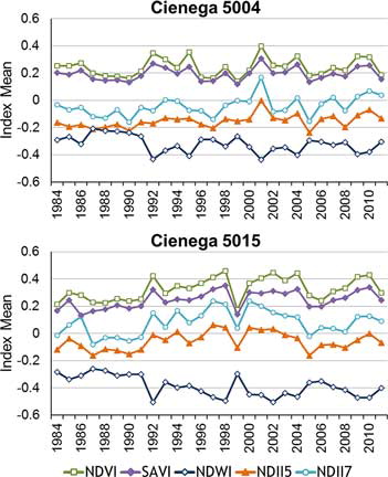
Figure 5. Spectral index trends from 1984 to 2011 showing the variability of trends. For any particular index, trends are highly variable between different cienegas ranging from strongly negative to strongly positive. Accounting for NDWI values being inversely related to the other indices, for any particular cienega the trends are much less variable, differing only in terms of degree. Cienega polygons are represented larger than actual size in order for all cienegas to be clearly visualized.

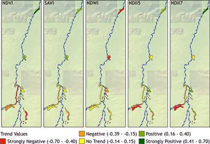
Table 4. Temporal trends in spectral indices for individual cienega areas, calculated as the slope of a linear regression fit to mean index value of each cienega for one Landsat scene per dry summer season, from 1984–2011. Only cienegas with at least one significant trend are reported. *Indicates cienegas affected by the Cienega Creek Cattle Exclosure. Italics indicates statistical significance (P < 0.05).

Cienega ID	NDVI	SAVI	NDWI	NDII5	NDII7
5001	−0.4	−0.3	0.0	−0.1	−0.2
5004	0.1	0.1	−0.3	0.3	0.4
5005	−0.5	−0.3	0.1	−0.3	−0.3
5006	−0.7	−0.5	0.3	−0.2	−0.3
5007	−0.5	−0.4	0.2	−0.1	−0.2
5010	−0.4	−0.3	0.0	−0.2	−0.3
5011	−0.6	−0.4	0.3	−0.1	−0.3
5012	0.1	0.1	−0.4	0.2	0.2
5013	0.0	0.0	−0.3	0.1	0.0
5015*	0.4	0.4	−0.6	0.2	0.4
5016	0.2	0.1	−0.4	0.0	0.1
5019	0.0	0.1	−0.3	0.1	0.1
5021	−0.5	−0.4	0.1	−0.5	−0.7
5026	0.3	0.2	−0.4	0.5	0.5
5029	−0.4	−0.3	−0.1	−0.5	−0.5
5031	−0.3	−0.2	−0.1	−0.4	−0.6
5038*	0.2	0.2	−0.5	0.0	0.0
5040*	0.5	0.4	−0.7	0.1	0.3
5042	−0.4	−0.3	0.0	0.0	−0.2
5043	−0.4	−0.3	0.1	0.0	−0.2
5044*	0.5	0.4	−0.6	0.4	0.5

Initial consideration of temporal trends suggested a spatial trend and Global Moran’s I was analyzed to evaluate clustering. All spectral index trends show a statistically significant clustered spatial pattern as determined by Moran’s I (Table 5). NDVI and SAVI trends are both strongly clustered (P = 0.000) and visually display a directional trend with positive trends in the north and closer to Cienega Creek while trends in the south and further from the creek are more negative. NDWI is strongly clustered (P = 0.000) and shows a directional trend that is strongly negative in the north and close to Cienega Creek while trends in the south and away from the creek are more moderate. NDII5 and NDII7 trends are also strongly clustered (P = 0.000) but no clear north-south spatial trend is apparent; several cienegas on the east side of Cienega Creek show positive trends.

Table 5. Moran’s I analysis of the spatial correlation of trends in spectral index values for cienegas through time.

	NDVI	SAVI	NDWI	NDII5	NDII7
Moran’s Index:	0.4525	0.4267	0.4284	0.2903	0.3923
p-value:	0.0000	0.0000	0.0000	0.0002	0.0000

Discussion and conclusions

The aforemenitoned research demonstrates that cienega and upland habitats can be readily distinguished from each other using a topographic data at 10 m spatial resolution or Landsat spectral data at 30 m spatial resolution. The TWI distinguished cienegas and riparian areas from upland areas. However, TWI does not reliably distinguish cienega from riparian areas because both are generally located within the valley bottom with similar topographic characteristics at the moderate spatial resolution used. One difference between the TWI and other examined indices is topographic data lacks the seasonal and interannual variability of spectral data at the time scale measured. Topographic variations that occur on a decadal scale and might affect cienega health may not be captured at the spatial resolution of most publicly available datasets. High spatial and temporal resolution topographic data, such as annual LiDAR, is becoming increasingly available and would provide an elevation model with higher resolution, which combined with the inclusion of hydrological sinks in the analysis may increase the performance of this index.

All spectral indices reliably distinguished cienega and riparian areas from upland habitats for all years included in the analysis. Of the five spectral indices, NDII5 most reliably distinguishes cienega from riparian habitat, most likely due to the sensitivity of SWIR (1.65 µm) in sensing different levels of plant canopy water content in wetland vegetation (Hunt and Rock 1989). Other studies have found this band useful in identifying open water in arid landscapes (Ozesmi and Bauer 2002; Soti et al. 2009; Campos, Sillero, and Brito 2012; Owen, Duncan, and Pettorelli 2015); this finding extends that research to include the utility of SWIR in identifying cienegas, which are wetlands areas with mixed cover types of vegetation, water and bare soil. NDII7 is the least reliable at distinguishing cienega from riparian habitat. Both TM band 5 and TM band 7 are sensitive to soil characteristics and soil salinity (Nield, Boettinger, and Ramsey 2007). The different sensitivities of the SWIR bands to the soil of Las Cienegas NCA may result in the different performance of NDII5 and NDII7 and soil characteristics should be considered when applying these indices to other regions. NDWI is the second most reliable in distinguishing cienega from riparian habitats. The two vegetation indices, NDVI and SAVI, were less capable of distinguishing cienega from riparian habitats than NDII5 or NDWI. The response of the NDWI, NDVI and SAVI could be related to management activities of the riparian corridor. Cattle exclosure fences were installed along Cienega Creek from 1984 to 2004, which resulted in a vegetation conversion from shrubland to forest along most of the riparian corridor. The change to a much higher canopy cover within the exclosure reduced the detectability of open water. NDWI and NDVI means showed no statistically significant differences between riparian and cienega areas until 1996; SAVI means showed no statistically significant differences between riparian and cienega areas until 1993. This change in ability of NDWI, NDVI, and SAVI to distinguish between cienega and riparian areas indicates that the gallery forest matured along most of the riparian zone by the mid-1990s.

All of the spectral indices examined are measures of water in some form: open water, vegetation moisture content, or photosynthetic activity. Temporal trends in these indices, especially at mesic sites such as cienegas, are going to respond to general precipitation trends in the area. However, differences in trends between cienegas and the considerable clustering of temporal trends for cienegas indicate that these spectral indices are affected by factors other than precipitation. The clustering of the vegetation and water indices shows a directional trend, generally north to south. A north-south general spatial trend corresponds to an elevation trend and hydrologic continuum; cienegas in the north also tend to be included in the Cienega Creek exclosure, which resulted in a vegetation community change and increased canopy cover. As canopy cover increased, open water detectable by satellite decreased which resulted in an increase in the vegetation indices while decreasing NDWI. Further analyses would determine the strength of the directional trend and may indicate to what extent factors other than canopy cover, such as elevation, hydrology and latitude, are involved. The infrared indices do not demonstrate the same directional trend. When considered with the results of the ANOVA, NDII5 may be less susceptible to the factors that are influencing this directional trend and therefore be a more robust measure of cienega habitat overall.

This research identified the most useful remote sensing index for general measures of cienega health but specific management goals may require different techniques for analysis. Since 2013, cienegas outside of the riparian channel have been fenced to exclose cattle. It is uncertain if these cienegas further from the riparian channel will experience the same vegetation community conversion that occurred along the riparian corridor since they are affected by different geomorphological and hydrological processes. Additionally, recent management activities do not focus on vegetation community conversion but instead focus on maintaining sections of open water for waterfowl use or increasing habitat for endangered species in these newly exclosed cienegas. When considering remote sensing techniques, managers must clearly identify goals for monitoring in order to effectively apply this technology. If tracking vegetation community conversion is the priority, then one of the vegetation indices (NDVI or SAVI) may be more appropriate but if the extent of open water is of interest then NDWI should be used. For some monitoring objectives, such as surface water infiltration or endangered species populations, remote sensing may not be able to replace field data collection. But to track overall cienega health through different vegetation community conversions and a variety of land management actions, NDII5 was the most effective index examined. Continued monitoring of cienega trends using NDII5 will provide information on the effects of recent and future management actions; this information can be included in an adaptive management strategy for cienega conservation.

In this study the location of the cienegas were known and those areas were compared against nearby non-cienegas areas to determine which index was most effective. To study areas where the location of cienegas is not known there are several methods that could be used to determine the distribution of cienegas. Aerial photography identification is a possibility dependent on several factors: the quality of the photos, season of survey, and format of photos (black and white or full color). Remote sensing classification is another possibility and this research indicates that NDII5 would be an important input for classification analysis. Pixel size can be a limiting factor in any satellite imagery analysis and, if available, higher resolution imagery with bands comparable to TM bands 4 and 5 would be useful in capturing smaller cienegas and more precisely defining cienega edges. Another remote sensing technique that could be used to study cienegas is spectral unmixing analysis. Endmember selection requires the knowledge of a number cienegas large enough to encompass a full pixel; this limits the application of spectral unmixing analysis to areas where cienega locations are already known. However, spectral unmixing analysis may offer the ability to track changes in the extent of cienegas over time using coarser resolution, publicly available imagery.

This research demonstrates the ability of remote sensing techniques to distinguish cienegas and monitor temporal changes in these unique habitats using publicly available Landsat TM imagery. NDII5 was the most effective index for general measure of cienega health in the semi-arid grasslands of the southwestern United States and should be further explored as a tool in assessing cienegas and remote sensing classification of cienega habitats. Broader application of NDII5 to monitor other wetland types is possible but certain habitat conditions, such as canopy cover, and the effect of management actions should be further researched.

Acknowledgments

We appreciate the peer review done by Jessica Walker, USGS; many thanks to Jeff Simms of the BLM and Gita Bodner of The Nature Conservancy for sharing their knowledge of and commitment to Las Cienegas NCA; and thank you to Chris Lukinbeal and the GIST program of the School of Geography and Development at the University of Arizona for help making our research a success. References to commercial vendors of software products or services are provided solely for the convenience of users when obtaining or using USGS software. Such references do not imply any endorsement by the U.S. Government.

References

- Adam, E., O. Mutanga, and D. Rugege. 2010. Multispectral and hyperspectral remote sensing for identification and mapping of wetland vegetation: A review. Wetlands Ecology and Management 18: 281–96. doi:10.1007/s11273-009-9169-z
- Arizona Department of Environmental Quality. 2008. Outstanding Arizona Waters (OAWs). Arizona Administrative Code R18–11–112(G).
- Ault, T. R., J. E. Cole, J. T. Overpeck, G. T. Pederson, and D. M. Meko. 2014. Assessing the risk of persistent drought using climate model simulations and paleoclimate data. Journal of Climate 27: 7529–49. doi:10.1175/jcli-d-12-00282.1
- Bannari, A., D. Morin, F. Bonn, and A. R. Huete. 1995. A review of vegetation indices. Remote Sensing Reviews 13: 95–120. doi:10.1080/02757259509532298b
- Beck, L. R., C. F. Hutchinson, and J. Zauderer. 1990. A comparison of greenness measures in two semi-arid grasslands. Climatic Change 17: 287–303. doi:10.1007/bf00138372
- Beven, K. J., and M. J. Kirkby. 1979. A physically based, variable contributing area model of basin hydrology / Un modèle à base physique de zone d’appel variable de l’hydrologie du bassin versant. Hydrological Sciences Bulletin 24: 43–69. doi:10.1080/02626667909491834
- Bodner, G., and K. Simms. 2008. State of the Las Cienegas National Conservation Area. Part 3. Condition and trend of riparian target species, vegetation and channel geomorphology. Tucson, AZ: The Nature Conservancy.
- Bodner, G., J. Simms, and D. Gori. 2007. State of the Las Cienegas National Conservation Area: Gila topminnow population status and trends 1989–2005. Tucson, AZ: The Nature Conservancy.
- Campos, J. C., N. Sillero, and J. C. Brito. 2012. Normalized difference water indexes have dissimilar performances in detecting seasonal and permanent water in the Sahara–Sahel transition zone. Journal of Hydrology 464–465: 438–46. doi:10.1016/j.jhydrol.2012.07.042
- Caves, J. K., G. S. Bodner, K. Simms, L. A. Fisher, and T. Robertson. 2013. Integrating collaboration, adaptive management, and scenario-planning: Experiences at Las Cienegas National Conservation Area. Ecology and Society 18: 43. doi:10.5751/es-05749-180343
- Cayan, D. R., T. Das, D. W. Pierce, T. P. Barnett, M. Tyree, and A. Gershunov. 2010. Future dryness in the southwest US and the hydrology of the early 21st century drought. Proceedings of the National Academy of Sciences 107: 21271–76. doi:10.1073/pnas.0912391107
- Chuvieco, E., D. Riaño, I. Aguado, and D. Cocero. 2002. Estimation of fuel moisture content from multitemporal analysis of Landsat Thematic Mapper reflectance data: Applications in fire danger assessment. International Journal of Remote Sensing 23: 2145–62. doi:10.1080/01431160110069818
- Daly, C., W. P. Gibson, G. H. Taylor, G. L. Johnson, and P. Pasteris. 2002. A knowledge-based approach to the statistical mapping of climate. Climate Research 22: 99–113. doi:10.3354/cr022099
- Dollison, R. M. 2010. The National Map: New viewer, services, and data download. Washington, DC: US Geological Survey [Fact Sheet 2010–3055].
- Dominguez, F., J. Cañon, and J. Valdes. 2009. IPCC-AR4 climate simulations for the Southwestern US: The importance of future ENSO projections. Climatic Change 99: 499–514. doi:10.1007/s10584-009-9672-5
- ESRI, DeLorme, and NAVTEQ. 2015a. Canvas/World_Light_Gray_Base. ESRI Basemaps. ESRI, Redlands, California, USA.
- ESRI, TomTom, U. S. Department of Commerce, U. S. Census Bureau, U. S. Department of Agriculture, and National Agricultural Statistics Service. 2015b. USA States. ESRI Layer Package. ESRI, Redlands, California, USA.
- Gao, B. 1996. NDWI – A normalized difference water index for remote sensing of vegetation liquid water from space. Remote Sensing of Environment 58: 257–66. doi:10.1016/s0034-4257(96)00067-3
- García, M. J. L., and V. Caselles. 1991. Mapping burns and natural reforestation using thematic Mapper data. Geocarto International 6: 31–37. doi:10.1080/10106049109354290
- Gori, D., and H. Schussman. 2005. State of the Las Cienegas National Conservation Area. Part I. Condition and trend of the desert grassland and watershed. Tucson, AZ: The Nature Conservancy.
- Grimm, N. B., A. Chacón, C. N. Dahm, S. W. Hostetler, O. T. Lind, P. L. Starkweather, and W. W. Wurtsbaugh. 1997. Sensitivity of aquatic ecosystems to climatic and anthropogenic changes: The basin and range, American southwest and Mexico. Hydrological Processes 11: 1023–41. doi:10.1002/(sici)1099-1085(19970630)11:8<1023::aid-hyp516>3.0.co;2-a
- Hardisky, M. A., F. C. Daiber, C. T. Roman, and V. Klemas. 1984. Remote sensing of biomass and annual net aerial primary productivity of a salt marsh. Remote Sensing of Environment 16: 91–106. doi:10.1016/0034-4257(84)90055-5
- Hardisky, M. A., V. Klemas, and R. M. Smart. 1983. The influence of soil salinity, growth form, and leaf moisture on the spectral radiance of spartina alterniflora canopies. Photogrammetric Engineering & Remote Sensing 49: 77–83.
- Hendrickson, D. A., and W. L. Minckley. 1984. Cienegas: Vanishing climax communities of the American Southwest. Desert Plants 6: 131–74.
- Huete, A. R. 1988. A soil-adjusted vegetation index (SAVI). Remote Sensing of Environment 25: 295–309. doi:10.1016/0034-4257(88)90106-x
- Huete, A. R., and R. D. Jackson. 1987. Suitability of spectral indices for evaluating vegetation characteristics on arid rangelands. Remote Sensing of Environment 23: 213–32. doi:10.1016/0034-4257(87)90038-1
- Huete, A. R., R. D. Jackson, and D. F. Post. 1985. Spectral response of a plant canopy with different soil backgrounds. Remote Sensing of Environment 17: 37–53. doi:10.1016/0034-4257(85)90111-7
- Hunt, E. R. Jr., and B. N. Rock. 1989. Detection of changes in leaf water content using Near- and Middle-Infrared reflectances. Remote Sensing of Environment 30: 43–54. doi:10.1016/0034-4257(89)90046-1
- Jackson, T. J., D. Chen, M. Cosh, F. Li, M. Anderson, C. Walthall, P. Doriaswamy, and E. R. Hunt. 2004. Vegetation water content mapping using Landsat data derived normalized difference water index for corn and soybeans. Remote Sensing of Environment 92: 475–82. doi:10.1016/j.rse.2003.10.021
- Ji, L., L. Zhang, B. K. Wylie, and J. Rover. 2011. On the terminology of the spectral vegetation index (NIR − SWIR)/(NIR + SWIR). International Journal of Remote Sensing 32: 6901–09. doi:10.1080/01431161.2010.510811
- Jones, K. B., C. E. Edmonds, E. T. Slonecker, J. D. Wickham, A. C. Neale, T. G. Wade, K. H. Riitters, and W. G. Kepner. 2008. Detecting changes in riparian habitat conditions based on patterns of greenness change: A case study from the Upper San Pedro River Basin, USA. Ecological Indicators 8: 89–99. doi:10.1016/j.ecolind.2007.01.001
- Justice, C. O., J. R. G. Townshend, B. N. Holben, and C. J. Tucker. 1985. Analysis of the phenology of global vegetation using meteorological satellite data. International Journal of Remote Sensing 6: 1271–318. doi:10.1080/01431168508948281
- Kerr, J. T., and M. Ostrovsky. 2003. From space to species: Ecological applications for remote sensing. Trends in Ecology & Evolution 18: 299–305. doi:10.1016/s0169-5347(03)00071-5
- Levene, H. 1961. Robust tests for equality of variances. In Contributions to probability and statistics. Essays in honor of Harold Hotelling, eds. I. Olkin S. G. Ghurye W. Hoeffding W. G. Madow and H. B. Mann 279–92. Standford, CA: Standford University Press.
- Magurran, A. E., S. R. Baillie, S. T. Buckland, J. M. Dick, D. A. Elston, E. M. Scott, R. I. Smith, P. J. Somerfield, and A. D. Watt. 2010. Long-term datasets in biodiversity research and monitoring: Assessing change in ecological communities through time. Trends in Ecology & Evolution 25: 574–82. doi:10.1016/j.tree.2010.06.016
- Mcfeeters, S. K. 1996. The use of the Normalized Difference Water Index (NDWI) in the delineation of open water features. International Journal of Remote Sensing 17: 1425–32. doi:10.1080/01431169608948714
- Minckley, T. A., and A. Brunelle. 2007. Paleohydrology and growth of a desert ciénega. Journal of Arid Environments 69: 420–31. doi:10.1016/j.jaridenv.2006.10.014
- Minckley, T. A., A. Brunelle, and D. Turner. 2013. Paleoenvironmental framework for understanding the development, stability, and state-changes of cienegas in the American deserts. USDA Forest Service Proceedings RMRS-P 67: 77–83.
- Minckley, T. A., D. S. Turner, and S. R. Weinstein. 2013. The relevance of wetland conservation in arid regions: A re-examination of vanishing communities in the American Southwest. Journal of Arid Environments 88: 213–21. doi:10.1016/j.jaridenv.2012.09.001
- Moeslund, J. E., L. Arge, P. K. Bøcher, T. Dalgaard, R. Ejrnæs, M. V. Odgaard, and J.-C. Svenning. 2013. Topographically controlled soil moisture drives plant diversity patterns within grasslands. Biodiversity and Conservation 22: 2151–66. doi:10.1007/s10531-013-0442-3
- Moran, P. A. P. 1948. The interpretation of statistical maps. Journal of the Royal Statistical Society. Series B (Methodological) 10: 243–51.
- Nagler, P. L., E. P. Glenn, and A. R. Huete. 2001. Assessment of spectral vegetation indices for riparian vegetation in the Colorado River delta, Mexico. Journal of Arid Environments 49: 91–110. doi:10.1006/jare.2001.0844
- Nguyen, U., E. P. Glenn, P. L. Nagler, and R. L. Scott. 2015. Long-term decrease in satellite vegetation indices in response to environmental variables in an iconic desert riparian ecosystem: The Upper San Pedro, Arizona, United States. Ecohydrology 8: 610–25. doi:10.1002/eco.1529
- Nield, S. J., J. L. Boettinger, and R. D. Ramsey. 2007. Digitally mapping gypsic and natric soil areas using landsat ETM data. Soil Science Society of America Journal 71: 245–52. doi:10.2136/sssaj2006-0049
- Norman, L., M. Villarreal, H. R. Pulliam, R. Minckley, L. Gass, C. Tolle, and M. Coe. 2014. Remote sensing analysis of riparian vegetation response to desert marsh restoration in the Mexican Highlands. Ecological Engineering 70: 241–54. doi:10.1016/j.ecoleng.2014.05.012
- Owen, H. J. F., C. Duncan, and N. Pettorelli. 2015. Testing the water: Detecting artificial water points using freely available satellite data and open source software. Remote Sensing in Ecology and Conservation 1: 61–72. doi:10.1002/rse2.5
- Ozesmi, S. L., and M. E. Bauer. 2002. Satellite remote sensing of wetlands. Wetlands Ecology and Management 10: 381–402.
- Perry, L. G., D. C. Andersen, L. V. Reynolds, S. M. Nelson, and P. B. Shafroth. 2012. Vulnerability of riparian ecosystems to elevated CO2 and climate change in arid and semiarid western North America. Global Change Biology 18: 821–42. doi:10.1111/j.1365-2486.2011.02588.x
- Rouse, J., R. Haas, J. Schell, and D. Deering. 1974. Monitoring vegetation systems in the great plains with ERTS. Washington, DC: National Aeronautics and Space Administration. National Aeronautics and Space Administration Special Publication 351:309.
- Sabo, J. L., R. Sponseller, M. Dixon, K. Gade, T. Harms, J. Heffernan, A. Jani, G. Katz, C. Soykan, J. Watts, and J. Welter. 2005. Riparian zones increase regional species richness by harboring different, not more, species. Ecology 86: 56–62. doi:10.1890/04-0668
- Seager, R., M. Ting, I. Held, Y. Kushnir, J. Lu, G. Vecchi, H.-P. Huang etal., 2007. Model projections of an imminent transition to a more arid climate in southwestern North America. Science 316: 1181–84. doi:10.1126/science.1139601
- Shoutis, L., D. T. Patten, and B. McGlynn. 2010. Terrain-based predictive modeling of riparian vegetation in a Northern Rocky Mountain Watershed. Wetlands 30: 621–33. doi:10.1007/s13157-010-0047-5
- Soti, V., A. Tran, J.-S. Bailly, C. Puech, D. L. Seen, and A. Bégué. 2009. Assessing optical earth observation systems for mapping and monitoring temporary ponds in arid areas. International Journal of Applied Earth Observation and Geoinformation 11: 344–51. doi:10.1016/j.jag.2009.05.005
- Stow, D., M. Niphadkar, and J. Kaiser. 2006. Time series of chaparral live fuel moisture maps derived from MODIS satellite data. International Journal of Wildland Fire 15: 347–60. doi:10.1071/wf05060
- Tamhane, A. C. 1977. Multiple comparisons in model i one-way anova with unequal variances. Communications in Statistics - Theory and Methods 6: 15–32. doi:10.1080/03610927708827466
- U. S. Congress. 2000. To establish the Las Cienegas National Conservation Area in the State of Arizona. Public Law 106–538.
- Villarreal, M. L., W. J. D. V. Leeuwen, and J. R. Romo-Leon. 2012. Mapping and monitoring riparian vegetation distribution, structure and composition with regression tree models and post-classification change metrics. International Journal of Remote Sensing 33: 4266–90. doi:10.1080/01431161.2011.644594
- Villarreal, M. L., L. M. Norman, K. G. Boykin, and C. S. A. Wallace. 2013. Biodiversity losses and conservation trade-offs: Assessing future urban growth scenarios for a North American trade corridor. International Journal of Biodiversity Science, Ecosystem Services & Management 9: 90–103. doi:10.1080/21513732.2013.770800
- Walford, N. 2011. Practical statistics for geographers and earth scientists. Chichester, UK: Wiley.
- Waters, M. R., and C. V. Haynes. 2001. Late quaternary arroyo formation and climate change in the American Southwest. Geology 29: 399–402. doi:10.1130/0091-7613(2001)029<0399:lqafac>2.0.co;2
- Wilson, E. H., and S. A. Sader. 2002. Detection of forest harvest type using multiple dates of Landsat TM imagery. Remote Sensing of the Environment 80: 385–96. doi:10.1016/s0034-4257(01)00318-2
- Wilson, N. R. 2014. A comparison of remote sensing indices and a temporal study of cienegas at cienega creek from 1984 to 2011 using multispectral satellite imagery. Tucson, AZ: University of Arizona.
- Yang, X. 2007. Integrated use of remote sensing and geographic information systems in riparian vegetation delineation and mapping. International Journal of Remote Sensing 28: 353–70. doi:10.1080/01431160600726763
- Zhang, C., and Y. Murayama. 2000. Testing local spatial autocorrelation using k-order neighbours. International Journal of Geographical Information Science 14: 681–92. doi:10.1080/136588100424972