High Phase Order Transmission Line Fault Types

Abstract

For high phase order (HPO) transmission systems, a major hurdle to overcome is the fault analysis and protection studies needed to guarantee successful implementation. This paper presents new equations which calculate the number of fault types and significant fault types of n-phase transmission lines. In addition, this paper defines and explains symmetrically significant fault types for HPO transmission systems. Lastly, this paper figuratively shows the significant fault types and symmetrically significant fault types for multiple HPO systems, n = 3, 4, 5, 6, 9, and 12. The equations and figures presented in this paper will assist in fault analysis and protective relay designs for HPO systems. The equations presented are used to determine the number of fault types a relay will need to account for, and the figurative approach shows the faults to be studied before HPO implementation.

Keywords:

• faults
• fault types
• fault current
• significant fault types
• symmetrically significant fault types
• high phase order
• six-phase
• nine-phase
• twelve-phase
• power systems
• transmission lines

1. Introduction

Electric energy demand in the long term is increasing and in the U.S. from 2012 to 2040 it is estimated that growth will be approximately 29% [1]. The increase in worldwide population, especially in urban areas causes difficulties obtaining rights of way for transmission assets. Much of the transmission infrastructure is a half century to a century old and in need of upgrading. One reference states that 70% of transmission lines and transformers are more than 25 years old [2]. There is an increase in transmission and distribution congestion due to many factors including deregulation of the power industry which deferred transmission and distribution investments [2] and [3]. In addition, there is an increase in natural gas and renewable generation sites causing an increase in transmission investments. Renewable portfolio standards will increase the renewable generation sites located far from load centers causing additional transmission to be constructed [4]. There are also regulations such as the Energy Policy Act of 2005 [5] and the American Recovery and Reinvestment Act of 2009 [6] which aim to promote transmission infrastructure with tax credits and methods to ease the transmission planning process. Overall between 2010 and 2030, the U.S. electric utility industry will put $1.5 to $2 trillion dollars in infrastructure investment [2].

With the large future investments in transmission systems and limited access to right of ways, high power density transmission designs will be necessary, one of which is high phase order (HPO) technologies, which have been proven to transfer more power for less right of way vs. their multi-circuit three-phase counterparts (e.g., double circuit three-phase vs. six-phase) [7].

One of the key problems implementing high phase order transmission is the protection strategies needed. High phase order fault analysis has been discussed in papers, e.g., [8]–[13]. HPO transmission systems have significantly more fault types than three-phase transmission systems. This in turn causes an increased range of fault currents to protect from, and more difficulties identifying, locating, and isolating faults. This paper’s contributions are

1. This paper presents new equations which calculate the number of fault types (FT) and significant (distinct) fault types (SFT) of n-phase transmission lines.

2. This paper also defines and explains symmetrically significant fault types (SSFT).

3. This paper shows an approach from a figurative perspective for example HPO systems to determine the faults that need to be analyzed and accounted for in HPO systems.

4. This paper shows every SFTs and SSFTs for n-phase systems for n = 3, 4, 5, 6, 9, and 12, which are often considered the most likely HPO designs [7] and [8].

The equations and figures presented in this paper will assist in protective relay designs for HPO systems. The equations will determine the number of fault types a relay will need to account for, and the figurative approach shows the faults to be studied before HPO implementation.

2. Fault Types

2.1. Fault Types

Fault types are defined as every fault that can occur on an n-phase system. For example, a three-phase line has 11 fault types:

• Phase A to ground,

• Phase B to ground,

• Phase C to ground,

• Phase A to B,

• Phase A to C,

• Phase B to C,

• Phase A to B to ground,

• Phase A to C to ground,

• Phase B to C to ground,

• Phase A to B to C,

• Phase A to B to C to ground.

One can immediately tell that the number of FTs for a HPO system is much larger than in the three-phase case.

The number of fault types has been presented for three-phase and six-phase [9, 11, 14]. However, an equation to calculate the number of fault types for any phase order system has not appeared in the literature. The number of fault types for n-phases is a combinatorial problem and can be represented as, (1) $$C_1^n+{2C}_2^n+\cdots {2C}_{n-1}^n+{2C}_n^n$$(1) where n is the number of phases. This is simplified to, (2) $$2\left(C_1^n+C_2^n+C_3^n+\cdots C_{n-1}^n+C_n^n\right)-n$$(2)

A known proof in the literature [15], which is the sum of the nth row of the binomial coefficients in Pascal’s triangle is (3) $$\sum _{0\le k\le n}{C}_k^n=2^n$$(3) and therefore, (4) $$\sum _{1\le k\le n}{C}_k^n=C_1^n+C_2^n+C_3^n+\cdots C_{n-1}^n+C_n^n=2^n-1$$(4)

Therefore Eq. (2(2) $$2\left(C_1^n+C_2^n+C_3^n+\cdots C_{n-1}^n+C_n^n\right)-n$$(2) ) simplifies to Eq. (5(5) $$F\left(n\right)=2^{n+1}-n-2$$(5) ), the number of fault types (F) for an n-phase system, (5) $$F\left(n\right)=2^{n+1}-n-2$$(5)

This can be proved through induction. First prove it is true for n = 1 from (2)(2) $$2\left(C_1^n+C_2^n+C_3^n+\cdots C_{n-1}^n+C_n^n\right)-n$$(2) , (6) $$F\left(1\right)=2\left(C_1^1\right)-n=1$$(6)

Assume n = k holds from Eq. (2(2) $$2\left(C_1^n+C_2^n+C_3^n+\cdots C_{n-1}^n+C_n^n\right)-n$$(2) ), (7) $$F\left(k\right)=2\left(C_1^k+C_2^k+C_3^k+\cdots C_{k-1}^k+C_k^k\right)-k$$(7)

Show n = k + 1 holds, (8) $$F\left(k+1\right)=2\left(C_1^{k+1}+C_2^{k+1}+C_3^{k+1}+\cdots C_k^{k+1}+C_{k+1}^{k+1}\right)-k-1$$(8)

Utilize Pascal’s formula [16] (9) $$C_c^{k+1}=C_c^k+C_{c-1}^k,$$(9)

Equation (8(8) $$F\left(k+1\right)=2\left(C_1^{k+1}+C_2^{k+1}+C_3^{k+1}+\cdots C_k^{k+1}+C_{k+1}^{k+1}\right)-k-1$$(8) ) can be written as (10) $$F\left(k+1\right)=2\left(C_0^k+C_1^k+C_1^k+C_2^k+C_2^k+C_3^k+\cdots \mathrm{}{C}_{k-1}^k+C_k^k+C_k^k+C_{k+1}^k\right)-k-1$$(10)

Reorganize, and note that, (11) $$C_0^k=1\text{and}{C}_{k+1}^k=0\mathrm{}$$(11) (12) $$F\left(k+1\right)=2\left(C_1^k+C_2^k+\cdots \mathrm{}{C}_{k-1}^k+C_k^k\right)-k+2\left(C_0^k+C_1^k+C_2^k+\cdots \mathrm{}{C}_{k-1}^k+C_k^k\right)-1$$(12)

The first part of Eq. (12(12) $$F\left(k+1\right)=2\left(C_1^k+C_2^k+\cdots \mathrm{}{C}_{k-1}^k+C_k^k\right)-k+2\left(C_0^k+C_1^k+C_2^k+\cdots \mathrm{}{C}_{k-1}^k+C_k^k\right)-1$$(12) ) is F(k), so, (13) $$F\left(k+1\right)=F\left(k\right)+2\left(C_0^k+C_1^k+C_2^k+\dots C_k^k\right)-1$$(13)

This is simplified using Eq. (3(3) $$\sum _{0\le k\le n}{C}_k^n=2^n$$(3) ), (14) $$F\left(k+1\right)=F\left(k\right)+2^{k+1}-1$$(14)

Plug (5(5) $$F\left(n\right)=2^{n+1}-n-2$$(5) ) in for F(k) in Eq. (14(14) $$F\left(k+1\right)=F\left(k\right)+2^{k+1}-1$$(14) ), (15) $$F\left(k+1\right)=2^{k+1}-2-k+2^{k+1}-1$$(15) (16) $$F\left(k+1\right)=2^{k+2}-k-3$$(16) (17) $$F\left(k+1\right)=2^{\left(k+1\right)+1}-(k+1)-2$$(17)

Therefore, Eq. (5)(5) $$F\left(n\right)=2^{n+1}-n-2$$(5) has been proven. The number of fault types for example n-phase systems from Eq. (5(5) $$F\left(n\right)=2^{n+1}-n-2$$(5) ) is in Table 1.

TABLE 1 The number of fault types, significant fault types, and symmetrically significant fault types for specified number of phases.

Number of phases	Fault types	Significant fault types	Symmetrically significant fault types
1	1	1	1
2	4	3	2
3	11	5	4
4	26	9	7
5	57	13	12
6	120	23	19
7	247	33	32
8	502	57	52
9	1013	89	86
10	2036	153	145
11	4083	249	248
12	8178	445	428
15	65,519	2445	2436

2.2. Significant Fault Types

It is important to note if HPO transmission lines were utilized, it would be more common on high-voltage long transmission lines, and uncommon for short distances, or distribution systems [17] and [18]. There is a break-even distance where HPO can be cost effect vs. three-phase or double circuit three-phase counterparts [17] and [18] (similar to HVDC lines). In addition, HPO systems have less unbalance than three-phase or double circuit three-phase over long distances [19]. This also means HPO may not need to be transposed for very long distances. In addition, if transposition is needed, it is much simpler than three-phase or double circuit three-phase [19].

Because of the substantial number of fault types in HPO circuits, techniques that simplify multiple solutions are desirable. When the types of faults that are analyzed by a common calculation yielding the same results (for balanced systems), are grouped, the resulting groups are termed the “significant fault types” (SFT). That is, certain types of faults can be grouped together because they require the same fault analysis on balanced systems. For example, in three-phase, the 11 FTs listed above can be simplified to five significant fault types:

• phase—ground

• phase—phase

• phase—phase—ground

• phase—phase—phase

• phase—phase—phase—ground.

Since HPO has an increased number of fault types, this simplification is especially desired. After grouping all the similar fault types that have identical analyses and fault currents, the number of significant fault types of an n-phase transmission line is much less than the number of fault types. An equation to calculate the number of SFTs for any phase order system has not appeared in the literature. The number of significant fault types for an n-phase system is (18) $$S\left(n\right)=c\left(n\right)-3+\frac{1}{n}\sum _{d|n}\mathit{phi}\left(d\right)2^{\frac{n}{d}}$$(18) (19) $$\mathrm{where}\mathrm{}c\left(n\right)=\left\{\begin{array}{l}\mathrm{f}\mathrm{o}\mathrm{r}\mathrm{}\mathrm{odd}\mathrm{}n:\mathrm{}{2}^{\frac{n-1}{2}+1}\\ \mathrm{f}\mathrm{o}\mathrm{r}\mathrm{}\mathrm{even}\mathrm{}n:\mathrm{}{2}^{\frac{n}{2}}+2^{\frac{n}{2}-1}\end{array}\right..$$(19)

The number of phasors is n. Note that the summation in Eq. (18(18) $$S\left(n\right)=c\left(n\right)-3+\frac{1}{n}\sum _{d|n}\mathit{phi}\left(d\right)2^{\frac{n}{d}}$$(18) ) is over all possible divisors d of n (all positive integers that divide evenly into n). For example for three-phase, d|3 results in the sum evaluated over d = 1, 3; d|12 results in the sum evaluated over d = 1, 2, 3, 4, 6, 12. Also, phi(d) is the Euler’s totient function also known as the “phi function,” which counts the totatives of d, i.e., the positive integers that are relatively prime to d, e.g., phi(9) counts numbers relatively prime to 9, i.e., phi(9) counts 1, 2, 4, 5, 7, and 8; that is 6 numbers: phi(9) = 6. Other examples are, phi(1) = 1, phi(2) = 1, phi(3) = 2, phi(4) = 2, and so forth. The author developed Eqs. (18)(18) $$S\left(n\right)=c\left(n\right)-3+\frac{1}{n}\sum _{d|n}\mathit{phi}\left(d\right)2^{\frac{n}{d}}$$(18) and (19)(19) $$\mathrm{where}\mathrm{}c\left(n\right)=\left\{\begin{array}{l}\mathrm{f}\mathrm{o}\mathrm{r}\mathrm{}\mathrm{odd}\mathrm{}n:\mathrm{}{2}^{\frac{n-1}{2}+1}\\ \mathrm{f}\mathrm{o}\mathrm{r}\mathrm{}\mathrm{even}\mathrm{}n:\mathrm{}{2}^{\frac{n}{2}}+2^{\frac{n}{2}-1}\end{array}\right..$$(19) from hand calculations counting the number of significant fault types for n-phase systems. A pattern was recognized, Eqs. (18(18) $$S\left(n\right)=c\left(n\right)-3+\frac{1}{n}\sum _{d|n}\mathit{phi}\left(d\right)2^{\frac{n}{d}}$$(18) ) and (19(19) $$\mathrm{where}\mathrm{}c\left(n\right)=\left\{\begin{array}{l}\mathrm{f}\mathrm{o}\mathrm{r}\mathrm{}\mathrm{odd}\mathrm{}n:\mathrm{}{2}^{\frac{n-1}{2}+1}\\ \mathrm{f}\mathrm{o}\mathrm{r}\mathrm{}\mathrm{even}\mathrm{}n:\mathrm{}{2}^{\frac{n}{2}}+2^{\frac{n}{2}-1}\end{array}\right..$$(19) ) were developed.

The number of SFTs is in Table 1 for n-phase systems for n = 1 to n = 15. A full example of these innovative equations is in Section 3 of this paper, and tables for the summation d|n and the phi function are in Tables 2 and 3. SFTs are discussed further in Section 4.

TABLE 2 The Phi function for d = 1 to d = 24.

d	Numbers relatively prime to d	phi(d)
1	1	1
2	1	1
3	1, 2	2
4	1, 3	2
5	1, 2, 3, 4	4
6	1, 5	2
7	1, 2, 3, 4, 5, 6	6
8	1, 3, 5, 7	4
9	1, 2, 4, 5, 7, 8	6
10	1, 3, 7, 9	4
11	1, 2, 3, 4, 5, 6, 7, 8, 9, 10	10
12	1, 5, 7, 11	4
13	1, 2, 3, 4, 5, 6, 7, 8, 9, 10, 11, 12	12
14	1, 3, 5, 9, 11, 13	6
15	1, 2, 4, 7, 8, 11, 13, 14	8
16	1, 3, 5, 7, 9, 11, 13, 15	8
17	1, 2, 3, 4, 5, 6, 7, 8, 9, 10, 11, 12, 13, 14, 15, 16	16
18	1, 5, 7, 11, 13, 17	6
19	1, 2, 3, 4, 5, 6, 7, 8, 9, 10, 11, 12, 13, 14, 15, 16, 17, 18	18
20	1, 3, 7, 9, 11, 13, 17, 19	8
21	1, 2, 4, 5, 8, 10, 11, 13, 16, 17, 19, 20	12
22	1, 3, 5, 7, 9, 13, 15, 17, 19, 21	10
23	1, 2, 3, 4, 5, 6, 7, 8, 9, 10, 11, 12, 13, 14, 15, 16, 17, 18, 19, 20, 21, 22	22
24	1, 5, 7, 11, 13, 17, 19, 23	8

2.3. Symmetrically Significant Fault Types

A select few of the significant fault types can be grouped together further. A SFT can be grouped with the corresponding SFT-to-ground if the sum of the faulted phasors is zero. For example, in a three-phase system, a phase—phase—phase fault has the same analysis and fault currents as a phase—phase—phase—ground fault in a balanced system; therefore, these two faults can be grouped and count as one “symmetrically significant fault type” (SSFT). SSFTs have not been discussed in the literature for HPO systems.

A SSFT only groups the multi-phase fault with the same multi-phase fault to ground. The grouping is only allowed when the fault is symmetric, i.e., the sum of the faulted phasors is zero, and due to this symmetry, the analysis for a fault and the same fault to ground are identical on balanced systems. The number of SSFTs is not much less than the number of SFTs. See Figure 1 for an example, this four-phase fault on a six-phase line is symmetric, and therefore the two SFTs can be grouped into one SSFT.

FIGURE 1. Symmetric significant fault type example. The four-phase fault and the four-phase fault to ground have the same fault analysis in balanced systems.

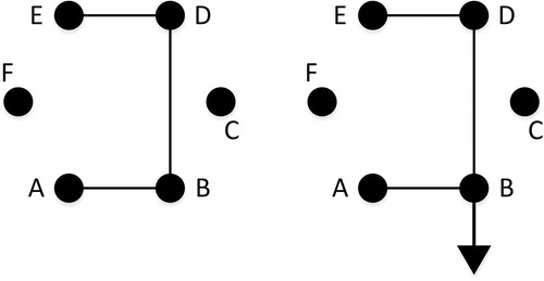
Note, the configuration does not have to be circular for this to hold true, as long as the line is balanced (long lines need to be transposed). For visualization, a circular configuration is useful. Transposition of HPO systems is explained further in [19].

Table 1 shows the number of SSFTs for n-phase systems for example HPO systems. SSFTs are discussed further in Section 4.

Note that all SSFTs need to be analyzed before an HPO line is implemented, and the relays need to account for all the fault currents from each SSFT. However, additional faults may need to be studied; when two separate simultaneous faults occur on the same line, e.g., fault on Phase A to ground and fault from Phase B to Phase C. Although rare, these faults are discussed in [10] and may need to be studied in addition to the SSFTs. Complex HPO fault analysis studies can be conducted utilizing software such as OpenDSS by the Electric Power Research Institute (EPRI).

3. Calculation of Number of Fault Types and Significant Fault Types Example

The math used in Eqs. (18(18) $$S\left(n\right)=c\left(n\right)-3+\frac{1}{n}\sum _{d|n}\mathit{phi}\left(d\right)2^{\frac{n}{d}}$$(18) ) and (19(19) $$\mathrm{where}\mathrm{}c\left(n\right)=\left\{\begin{array}{l}\mathrm{f}\mathrm{o}\mathrm{r}\mathrm{}\mathrm{odd}\mathrm{}n:\mathrm{}{2}^{\frac{n-1}{2}+1}\\ \mathrm{f}\mathrm{o}\mathrm{r}\mathrm{}\mathrm{even}\mathrm{}n:\mathrm{}{2}^{\frac{n}{2}}+2^{\frac{n}{2}-1}\end{array}\right..$$(19) ) is not seen anywhere else in the power systems community to the authors knowledge, i.e., the phi function (Table 2) and the summation over all possible divisors d of n (Table 3). For this reason, a brief example will be shown. For a 24-phase transmission line (n = 24), the calculations for the number of fault types and significant fault types are shown.

TABLE 3 The summation over d|n examples.

n	Positive integers that divide into n evenly
1	1
2	1, 2
3	1, 3
4	1, 2, 4
5	1, 5
6	1, 2, 3, 6
7	1, 7
8	1, 2, 4, 8
9	1, 3, 9
10	1, 2, 5, 10
11	1, 11
12	1, 2, 3, 4, 6, 12
13	1, 13
14	1, 2, 7, 14
15	1, 3, 5, 15
16	1, 2, 4, 8, 16
17	1, 17
18	1, 3, 6, 9, 18
19	1, 19
20	1, 2, 5, 10, 20
21	1, 3, 7
22	1, 2, 11, 22
23	1, 23
24	1, 2, 3, 4, 6, 8, 12, 24

The number of fault types from Eq. (5(5) $$F\left(n\right)=2^{n+1}-n-2$$(5) ) is $$F=2^{24+1}-2-24=33,554,406$$

The number of significant fault types form Eqs. (18(18) $$S\left(n\right)=c\left(n\right)-3+\frac{1}{n}\sum _{d|n}\mathit{phi}\left(d\right)2^{\frac{n}{d}}$$(18) ) and (19(19) $$\mathrm{where}\mathrm{}c\left(n\right)=\left\{\begin{array}{l}\mathrm{f}\mathrm{o}\mathrm{r}\mathrm{}\mathrm{odd}\mathrm{}n:\mathrm{}{2}^{\frac{n-1}{2}+1}\\ \mathrm{f}\mathrm{o}\mathrm{r}\mathrm{}\mathrm{even}\mathrm{}n:\mathrm{}{2}^{\frac{n}{2}}+2^{\frac{n}{2}-1}\end{array}\right..$$(19) ) is $$S=2^{\frac{24}{2}}+2^{\frac{24}{2}-1}-3+\frac{1}{24}\sum _{d|24}\mathit{phi}\left(d\right)2^{\frac{24}{d}}$$ $$S=2^{\frac{n}{2}}+2^{\frac{n}{2}-1}-3+\mathrm{}\frac{1}{n}\left(\mathit{phi}\left(1\right)2^{\frac{n}{1}}+\mathit{phi}\left(2\right)2^{\frac{n}{2}}+\mathit{phi}\left(3\right)2^{\frac{n}{3}}+\mathit{phi}\left(4\right)2^{\frac{n}{4}}+\mathit{phi}\left(6\right)2^{\frac{n}{6}}+\mathit{phi}\left(8\right)2^{\frac{n}{8}}+\mathit{phi}\left(12\right)2^{\frac{n}{12}}+\mathit{phi}\left(24\right)2^{\frac{n}{24}}\right)$$ $$S=6141+\frac{1}{24}\left(\left(1\right)2^{24}+\left(1\right)2^{12}+\left(2\right)2^8+\left(2\right)2^6+\left(2\right)2^4+\left(4\right)2^3+\left(4\right)2^2+\left(8\right)2^1\right)$$ $$S=705,393$$

4. Figurative Approach to SFTs and SSFTs

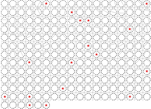
The significant fault types for a three-phase transmission line are well known and can be shown figuratively for a better understanding in Figure 2. The significant fault types for other numbers of phases are not well known, therefore examples are presented here and are shown figuratively in Figures 3–7. The phase to ground diagrams are not shown in Figures 3–7, since they are duplicative of the phase–phase diagrams with an added ground component. The significant fault types with a “star” next to them are symmetric, therefore the fault is the same as the fault to ground on a balanced system. Figures 3–7 show the SFTs and SSFTs for 4-phase, 5-phase, 6-phase, 9-phase, and 12-phase, respectively. Note that if HPO were used for power transmission lines, the most probable designs would be in multiples of three to allow for simpler conversion to 3-phase; therefore 6-phase, 9-phase and 12-phase are shown [8].

FIGURE 2. The SFTs for three-phase transmission lines. The fault with a “star” next to it is symmetric, i.e., the fault is the same as the fault to ground.

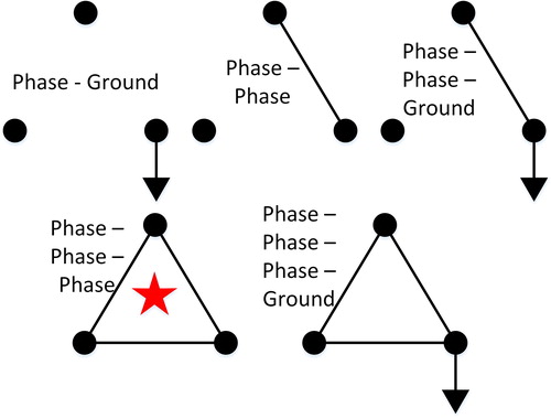
FIGURE 3. The four-phase SFTs. Five SFTs are not shown. Four not shown are identical to these four but also to ground. The last not shown is one phase to ground. The faults with a “star” next to it are symmetric, i.e., the fault is the same as the fault to ground.

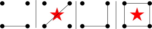
FIGURE 4. The five-phase SFTs. Seven SFTs are not shown. Six not shown are identical to these six but also to ground. The last not shown is one phase to ground. The fault with a “star” next to it is symmetric, i.e., the fault is the same as the fault to ground.

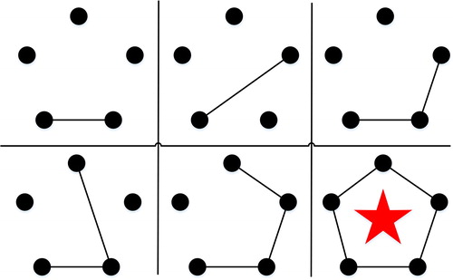
FIGURE 5. The six-phase SFTs. 12 SFTs are not shown. 11 not shown are identical to these 11 but also to ground. The last not shown is one phase to ground. The faults with a “star” next to it are symmetric, i.e., the fault is the same as the fault to ground.

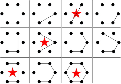
FIGURE 6. The nine-phase significant fault types. 45 significant fault types are not shown. 44 not shown are identical to these 44 but also to ground. The last not shown is one phase to ground. The faults with a “star” next to it are symmetric, i.e., the fault is the same as the fault to ground.

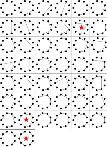
FIGURE 7. The twelve-phase significant fault types. 223 significant fault types are not shown. 222 not shown are identical to these 222 but also to ground. The last not shown is one phase to ground. The faults with a “star” next to it are symmetric, i.e., the fault is the same as the fault to ground.

The way in which Figures 2–7 would be utilized, is if the faults of an n-phase transmission line were to be studied; all the faults shown in the figure, relative to the number of phases, need to be analyzed. For example, take Figure 3, a four-phase transmission line, with Phase A, B, C, and D,

• a phase to nearest phase needs to be studied, such as a Phase A to Phase B fault, and its corresponding Phase A to Phase B to ground fault,

• a phase to opposite phase needs to be studied, such as Phase A to Phase C. Its corresponding Phase A to Phase C to ground fault does not need to be studied because this fault type is symmetric (indicated by the “star”).

• a phase to phase to phase fault needs to be studied, such as a Phase A to Phase B to Phase C fault, and its corresponding Phase A to Phase B to Phase C to ground fault.

• an all phase fault needs to be studied, Phase A to Phase B to Phase C to Phase D, but the corresponding fault to ground does not need to be studied because this is a symmetric fault.

• a phase to ground fault needs to be studied, e.g., a Phase A to ground fault. This is not shown in the figures, but always needs to be studied no matter the number of phases and is the most common type of fault.

The methods and equations described in this paper have been coded in MATLAB and the number of FTs, SFTs, and SSFTs can be determined for any n-phase system. In addition, the MATLAB code results in a list of all the FTs, SFTs, and SSFTs. If any readers would like access to this code, please email the author.

5. High Phase Order Fault Analysis Example

The equations developed in Section 2 and the figurative approach depicting the SFTs and SSFTs in Section 3 are meant to help with HPO transmission line fault analysis, which is an important part in the protection planning for HPO systems. Fault analysis and fault location detection for high phase order systems are complete research topics on their own. Fault analysis for 6-phase and 12-phase systems are studied in [7]–[14]. Fault location detection for HPO is a topic for future research and is briefly studied in [13], [20], and [21]. When determining fault location on HPO systems, extensions of three-phase methods could be utilized [22].

A simple per unit six-phase fault analysis example is shown here using generalized sequence components [23], for more detail fault analysis on HPO systems the readers are pointed to [7]–[14]. For the generalized case, assumptions are made that there is zero fault impedance, and the load current is much less than the fault current. Therefore, the prefault load current is assumed to be zero. It is also assumed line impedances are balanced.

For a generalized per unit six-phase example, a single-phase to neutral fault occurs on phase F. The prefault and postfault per unit voltage is $$V_{\mathit{abc}}^{\mathit{pre}}=\left[\begin{array}{c}\begin{array}{c}{1}^{}\\ b^5\\ b^4\end{array}\\ \begin{array}{c}{b}^3\\ b^2\\ b^{}\end{array}\end{array}\right].\mathrm{}{V}_{\mathit{abc}}^{\mathit{post}}=\left[\begin{array}{c}\begin{array}{c}{V}_a^{\mathit{post}}\\ V_b^{\mathit{post}}\\ V_c^{\mathit{post}}\end{array}\\ \begin{array}{c}{V}_d^{\mathit{post}}\\ V_e^{\mathit{post}}\\ 0\end{array}\end{array}\right],$$

The subscripts and superscripts abc represent the phase components, seq represents sequence components, pre represents prefault conditions, and post represents postfault conditions. Using the line impedance modal matrix T, where b is 1/60^°, the prefault and postfault sequence voltage is, $$V_{\mathit{seq}}^{\mathit{pre}}=T^{-1}{V}_{\mathit{abc}}^{\mathit{pre}}=\frac{1}{\sqrt{6}}{\left[\begin{array}{cc}\begin{array}{ccc}1& 1& 1\\ 1& b^5& b^4\\ 1& b^4& b^2\end{array}& \begin{array}{ccc}1& 1& 1\\ b^3& b^2& b^{}\\ 1^{}& b^4& b^2\end{array}\\ \begin{array}{ccc}1& b^3& 1^{}\\ 1& b^2& b^4\\ 1& b^{}& b^2\end{array}& \begin{array}{ccc}{b}^3& 1^{}& b^3\\ 1^{}& b^2& b^4\\ b^3& b^4& b^5\end{array}\end{array}\right]}^{-1}\left[\begin{array}{c}\begin{array}{c}{1}^{}\\ b^5\\ b^4\end{array}\\ \begin{array}{c}{b}^3\\ b^2\\ b^{}\end{array}\end{array}\right]=\left[\begin{array}{c}\begin{array}{c}0\\ \sqrt{6}\\ 0\end{array}\\ \begin{array}{c}0\\ 0\\ 0\end{array}\end{array}\right].$$ $$V_{\mathit{seq}}^{\mathit{post}}=T^{-1}{V}_{\mathit{abc}}^{\mathit{post}}=\frac{1}{\sqrt{6}}{\left[\begin{array}{cc}\begin{array}{ccc}1& 1& 1\\ 1& b^5& b^4\\ 1& b^4& b^2\end{array}& \begin{array}{ccc}1& 1& 1\\ b^3& b^2& b^{}\\ 1^{}& b^4& b^2\end{array}\\ \begin{array}{ccc}1& b^3& 1^{}\\ 1& b^2& b^4\\ 1& b^{}& b^2\end{array}& \begin{array}{ccc}{b}^3& 1^{}& b^3\\ 1^{}& b^2& b^4\\ b^3& b^4& b^5\end{array}\end{array}\right]}^{-1}\left[\begin{array}{c}\begin{array}{c}{V}_a^{\mathit{post}}\\ V_b^{\mathit{post}}\\ V_c^{\mathit{post}}\end{array}\\ \begin{array}{c}{V}_d^{\mathit{post}}\\ V_e^{\mathit{post}}\\ 0\end{array}\end{array}\right]=\frac{1}{\sqrt{6}}\left[\begin{array}{l}\begin{array}{c}{V}_a^{\mathit{post}}+V_b^{\mathit{post}}+V_c^{\mathit{post}}+V_d^{\mathit{post}}+V_e^{\mathit{post}}\\ V_a^{\mathit{post}}+{bV}_b^{\mathit{post}}+{b^{2}V}_c^{\mathit{post}}+{b^{3}V}_d^{\mathit{post}}+b^4{V}_e^{\mathit{post}}\\ V_a^{\mathit{post}}+{b^{2}V}_b^{\mathit{post}}+b^4{V}_c^{\mathit{post}}+V_d^{\mathit{post}}+{b^{2}V}_e^{\mathit{post}}\end{array}\\ \begin{array}{c}{V}_a^{\mathit{post}}+{b^{3}V}_b^{\mathit{post}}+V_c^{\mathit{post}}+{b^{3}V}_d^{\mathit{post}}+V_e^{\mathit{post}}\\ V_a^{\mathit{post}}+{b^{4}V}_b^{\mathit{post}}+{b^{2}V}_c^{\mathit{post}}+V_d^{\mathit{post}}+{b^{4}V}_e^{\mathit{post}}\\ V_a^{\mathit{post}}+{b^{5}V}_b^{\mathit{post}}+{b^{4}V}_c^{\mathit{post}}+{b^{3}V}_d^{\mathit{post}}+{b^{2}V}_e^{\mathit{post}}\end{array}\end{array}\right].$$

The postfault current in phase components and sequence components respectively are, $$I_{\mathit{abc}}^{\mathit{post}}=\left[\begin{array}{c}\begin{array}{c}0\\ 0\\ 0\end{array}\\ \begin{array}{c}0\\ 0\\ I_F\end{array}\end{array}\right]\mathrm{}{I}_{\mathit{seq}}^{\mathit{post}}=T^{-1}{I}_{\mathit{abc}}^{\mathit{post}}=\frac{1}{\sqrt{6}}\left[\begin{array}{c}\begin{array}{c}{I}_F\\ {b^{5}I}_F\\ b^4{I}_F\end{array}\\ \begin{array}{c}{b^{3}I}_F\\ {b^{2}I}_F\\ {bI}_F\end{array}\end{array}\right].$$

For a bolted fault at phase F, there is zero postfault voltage for phase F. It is assumed that there is only one nonzero postfault current and this is at phase F. Assuming a fully transposed system, where Z_S is the self-impedance and Z_mij is the mutual impedance, the line impedance matrix and the sequence component impedance matrix are $$Z_{\mathit{abc}}=\left[\begin{array}{cc}\begin{array}{ccc}{Z}_S& Z_{m12}& Z_{m13}\\ Z_{m12}& Z_S& Z_{m23}\\ Z_{m13}& Z_{m23}& Z_S\end{array}& \begin{array}{ccc}{Z}_{m14}& Z_{m15}& Z_{m16}\\ Z_{m24}& Z_{m25}& Z_{m26}\\ Z_{m34}& Z_{m35}& Z_{m36}\end{array}\\ \begin{array}{ccc}{Z}_{m14}& Z_{m24}& Z_{m34}\\ Z_{m15}& Z_{m25}& Z_{m35}\\ Z_{m16}& Z_{m26}& Z_{m36}\end{array}& \begin{array}{ccc}{Z}_S& Z_{m45}& Z_{m46}\\ Z_{m45}& Z_S& Z_{m56}\\ Z_{m46}& Z_{m56}& Z_S\end{array}\end{array}\right]\mathrm{}{Z}_{\mathit{seq}}=\mathit{diag}\left[\begin{array}{c}\begin{array}{c}{Z}_s+2Z_{m1}+2Z_{m2}+Z_{m3}\\ Z_s+Z_{m1}-Z_{m2}-Z_{m3}\\ Z_s-Z_{m1}-Z_{m2}+Z_{m3}\end{array}\\ \begin{array}{c}\mathrm{}{Z}_s-2Z_{m1}+2Z_{m2}-Z_{m3}\\ \mathrm{}{Z}_s-Z_{m1}-Z_{m2}+Z_{m3}\\ Z_s+Z_{m1}-Z_{m2}-Z_{m3}\end{array}\end{array}\right]$$ where all Z_mij are equal due to a balanced system.

Utilizing the previously determined matrices and setting values for the self and mutual impedances, self-impedance = j0.133 (R = 0) and all mutual impedances = j0.0333 (per unit), the six unknowns (postfault voltages and fault current) can be solved simultaneously from, $$V_{\mathit{seq}}^{\mathit{post}}=Z_{6seq}{I}_{\mathit{seq}}^{\mathit{post}}+V_{\mathit{seq}}^{\mathit{pre}}$$ $$\left[\begin{array}{c}\begin{array}{c}{V}_a^{\mathrm{p}\mathit{ost}}+V_b^{\mathit{post}}+V_c^{\mathit{post}}+V_d^{\mathit{post}}+V_e^{\mathit{post}}\\ V_a^{\mathit{post}}+{bV}_b^{\mathit{post}}+{b^{2}V}_c^{\mathit{post}}+{b^{3}V}_d^{\mathit{post}}+b^4{V}_e^{\mathit{post}}\\ V_a^{\mathit{post}}+{b^{2}V}_b^{\mathit{post}}+b^4{V}_c^{\mathit{post}}+V_d^{\mathit{post}}+{b^{2}V}_e^{\mathit{post}}\end{array}\\ \begin{array}{c}{V}_a^{\mathit{post}}+{b^{3}V}_b^{\mathit{post}}+V_c^{\mathit{post}}+{b^{3}V}_d^{\mathit{post}}+V_e^{\mathit{post}}\\ V_a^{\mathit{post}}+{b^{4}V}_b^{\mathit{post}}+{b^{2}V}_c^{\mathit{post}}+V_d^{\mathit{post}}+{b^{4}V}_e^{\mathit{post}}\\ V_a^{\mathit{post}}+{b^{5}V}_b^{\mathit{post}}+{b^{4}V}_c^{\mathit{post}}+{b^{3}V}_d^{\mathit{post}}+{b^{2}V}_e^{\mathit{post}}\end{array}\end{array}\right]=\mathit{diag}\left[\begin{array}{c}\begin{array}{c}{Z}_s+2Z_{m1}+2Z_{m2}+Z_{m3}\\ Z_s+Z_{m1}-Z_{m2}-Z_{m3}\\ Z_s-Z_{m1}-Z_{m2}+Z_{m3}\end{array}\\ \begin{array}{c}\mathrm{}{Z}_s-2Z_{m1}+2Z_{m2}-Z_{m3}\\ \mathrm{}{Z}_s-Z_{m1}-Z_{m2}+Z_{m3}\\ Z_s+Z_{m1}-Z_{m2}-Z_{m3}\end{array}\end{array}\right]\left[\begin{array}{c}\begin{array}{c}{I}_F\\ {b^{5}I}_F\\ b^4{I}_F\end{array}\\ \begin{array}{c}{b^{3}I}_F\\ {b^{2}I}_F\\ {bI}_F\end{array}\end{array}\right]+\left[\begin{array}{c}\begin{array}{c}0\\ 6\\ 0\end{array}\\ \begin{array}{c}0\\ 0\\ 0\end{array}\end{array}\right].$$ $$\left[\begin{array}{c}\begin{array}{c}{V}_a^{\mathit{post}}\\ V_b^{\mathit{post}}\\ V_c^{\mathit{post}}\end{array}\\ \begin{array}{c}{V}_d^{\mathit{post}}\\ V_e^{\mathit{post}}\\ I_F\end{array}\end{array}\right]=\left[\begin{array}{c}\begin{array}{c}0.90\mathrm{\angle }{-14}^o\\ 1.15\mathrm{\angle }{-71}^o\\ 1.25\mathrm{\angle }{-120}^o\end{array}\\ \begin{array}{c}1.15\mathrm{\angle }{-169}^o\\ 0.90\mathrm{\angle }{134}^o\\ 7.5\mathrm{\angle }{150}^o\end{array}\end{array}\right].$$

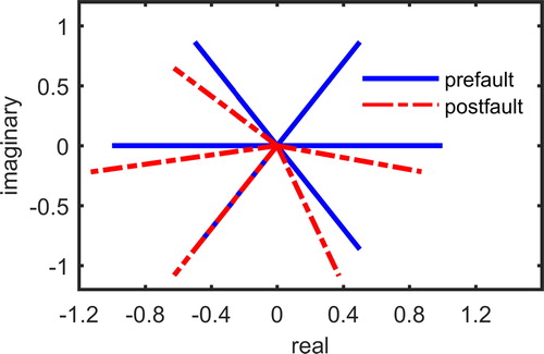
This solution can be viewed in a phasor diagram of the postfault and prefault phase voltages in Fig. 8.

FIGURE 8. Fault analysis phasor diagram of prefault voltages and postfault voltages after a phase to neutral fault on phase F for a simple six-phase fault analysis example. Phase variables are depicted.

6. Conclusions

This paper presents new equations, which have not been seen in the literature, to calculate the number of “fault types” and number of “significant fault types” of n-phase transmission lines. This paper extends research in [9] and [11], and [14] which discuss fault types and significant fault types for three-phase and six-phase designs; this paper creates an n-phase generalized equation for the number of fault types and significant fault types. In addition, this paper shows a figurative approach to the significant fault types. Lastly, “symmetrically significant fault types” for HPO systems is explained and this is not discussed in the literature for HPO systems. Multiple examples of the “significant fault types” and “symmetrically significant fault types” for the most probable HPO designs are shown, i.e., 4-phase, 5-phase, 6-phase, 9-phase, and 12-phase. The contributions of this work are only one part of a much larger problem to fault analysis and protection of high phase order transmission systems. The equations, methods, and figures presented in this paper will assist with fault analysis and relay protection designs for high phase order transmission systems.

Acknowledgements

The author would like to acknowledge the contributions of the author’s Ph.D. advisor Dr. Gerald T. Heydt from Arizona State University. Sandia National Laboratories is a multimission laboratory managed and operated by National Technology and Engineering Solutions of Sandia, LLC, a wholly owned subsidiary of Honeywell International, Inc., for the U.S. Department of Energy’s National Nuclear Security Administration under contract DE-NA0003525. The views expressed in the article do not necessarily represent the views of the U.S. Department of Energy or the United States Government.

Additional information

Notes on contributors

Brian J. Pierre

Brian J. Pierre holds a B.S. degree in electrical engineering from Boise State University, Boise, ID, USA; and an M.S. and Ph.D. in electrical engineering from Arizona State University focused on electric power systems, Tempe, AZ, USA. His dissertation focused in part on high phase order systems. He is presently a Senior Member of Technical Staff in the Electric Power Systems Research Department at Sandia National Laboratories, Albuquerque, NM, USA. His research interests and expertise include power system modeling, power transmission systems, power system controls, renewable energy integration, power system resilience, and power system optimization.

References

- U.S. Energy Information Administration. “Annual energy outlook 2014 with projections to 2040,” April, 2014.
- H. Williams, “Transmission & distribution infrastructure,” White Paper. Harris Williams & Co. Ltd, Richmond, VA, Summer 2010.
- K. Bannerjee, and R. Gorur, “Evaluating critical parameters of composite cores for high temperature low sag conductors for power delivery,” Power Systems Engineering Research Center, Final Project Report T-47, August, 2014.
- K. Cory, and B. Guery, “Renewable portfolio standards in the states: Balancing goals and implementation strategies,” Technical Report. National Renewable Energy Laboratory, Denver, CO, December, 2007.
- United State of America 109th Congress “Energy Policy Act of 2005,” Public Law 109-58. Washington DC, August, 2005.
- United State of America 111th Congress “American Recovery and Reinvestment Act,” Public Law 111-5. Washington DC, September, 2009.
- N. Bhatt, S. Venkata, W. Guyker, and W. Booth, “Six-phase (multi-phase) power transmission systems: Fault analysis,” IEEE Trans. Power Apparat. Syst., vol. 96, no. 3, pp. 758–767, 1977. DOI: 10.1109/T-PAS.1977.32389.
- B. Pierre, “Algorithm and model development for innovative high power AC transmission,” Dissertation, Arizona State University, 2015.
- S. Venkata, W. Guyker, J. Kondragunta, N. Saini, and E. Stanek, “138-kV, six-phase transmission system: Fault analysis,” IEEE Trans. Power Apparat. Syst., vol. 101, no. 5, pp. 1203–1218, 1982. DOI: 10.1109/TPAS.1982.317382.
- B. Bhat, and R. Sharma, “Analysis of simultaneous ground and phase faults on a six phase power system,” IEEE Trans. Power Del., vol. 4, no. 3, pp. 1610–1616, 1989. DOI: 10.1109/61.32650.
- Y. Song, A. Johns, and R. Aggarwal, “Digital simulation of fault transients on six-phase transmission systems,” Proc. IEE 2nd International Conference on Advances in Power System Control. Operation and Management, Hong Kong, 1993.
- E. Badawy, M. El-Sherbiny, A. Ibrahim, and M. Farghaly, “A method of analyzing unsymmetrical faults on six-phase power systems,” IEEE Trans. Power Del., vol. 6, no. 3, pp. 1139–1145, 1991. DOI: 10.1109/61.85859.
- C. Fan, L. Liu, and Y. Tian, “A fault-location method for 12-phase transmission lines based on twelve-sequence-component method,” IEEE Trans. Power Del., vol. 26, no. 1, pp. 135–142, 2011. DOI: 10.1109/TPWRD.2010.2079337.
- R. Rebbapragada, H. Panke, H. Pierce, J. Stewart, and L. Oppel, “Selection and application of relay protection for six phase demonstration project,” IEEE Trans. Power Del., vol. 7, no. 4, pp. 1900–1911, 1992. DOI: 10.1109/61.156993.
- D. Mazur, Combinatorics: A Guided Tour. Washington DC, USA: Mathematical Association of America, 2010, p. 61.
- R. Merris, Combinatorics. Hoboken, NJ: John Wiley, 2003, pp. 11–16.
- J. Bortnik, Transmission Line Compaction Using High Phase Order Transmission. Johannesburg, South Africa: University of Witwatersrand Johannesburg, 1998.
- E. Krizauskas, T. Landers, R. Richeda, L. Oppel, and J. Stewart, “High phase order transmission demonstration,” New York State Electric & Gas Corporation, Empire State Electric Energy Research Corporation, Albany, NY, Rep. EP 88-23-Phases 3 & 4, 1997.
- B. Pierre, and G. Heydt, “Transposition and voltage unbalance in high phase order power transmission systems,” Electr Power Compo Syst., vol. 42, no. 15, pp. 1754–1761, 2014. DOI: 10.1080/15325008.2014.949915.
- E. Koley, A. Jain, A. S. Thoke, A. Jain, and S. Ghosh, “Detection and classification of faults on six phase transmission line using ANN,” Proceedings International Conference on Computer & Communication Technology, Allahabad, India, 2011.
- A. Hajjar, and M. Mansour, “A microprocessor and wavelets based relaying approach for on line six-phase transmission lines protection,” Proceedings of the 41st International Universities Power Engineering Conference, Newcastle-upon-Tyne, UK, 2006.
- H. H. Goh et al., “Fault location techniques in electric power system: A review,” Indonesian j. elect. Eng. Comput. Sci., vol. 8, no. 1, pp. 206–212, 2017. DOI: 10.11591/ijeecs.v8.i1.pp206-212.
- G. T. Heydt, and B. J. Pierre, “Sequence impedances for high phase order power transmission systems,” Proceedings IEEE/PES Transmission and Distribution Conference and Exposition (T&D), Dallas, TX, USA, 2016.