High order concentrated matrix-exponential distributions

Abstract

This paper presents matrix-exponential (ME) distributions, whose squared coefficient of variation (SCV) is very low. Currently, there is no symbolic construction available to obtain the most concentrated ME distributions, and the numerical optimization-based approaches to construct them have many pitfalls. We present a numerical optimization-based procedure which avoids numerical issues.

Keywords:

• Coefficient of variation
• matrix-exponential distributions
• non-negative matrix-exponential functions
• numerical optimization

1. Introduction

Highly concentrated matrix-exponential functions play an important role in many research fields, for example, they turned out to be essential for numerical inverse Laplace transform methods as well.^[8]

The least varying phase type (PH) distribution of order N is known to be the Erlang distribution^[1] with SCV=$1/N$ (defined as $\frac{{\mu }_0{\mu }_2}{{\mu }_1^2}-1,$ where ${\mu }_i,i\in \{0,1,2\},$ are the moments of the distribution). Much less is known about the least varying ME distribution for order N. It is known that for order 2 the class of ME distributions is identical to the class of PH distributions, and it is also known that there exists an order 3 ME distribution with SCV = $0.200902<1/3,$ but it is still only a conjecture that this is the least varying order 3 ME distribution. Concentrated ME distributions are provided in Éltető et al.^[4] up to order 17 and in Horváth et al.^[7] up to order 47. These preliminary results indicate that, as N increases, the minimal SCV of order N ME distributions tends to be less than $2/N^2$ for odd N, and for even N, the minimal SCV is close to the minimal SCV of order N – 1 ME distributions. In this paper, we propose numerical procedures by which much higher odd order concentrated ME distributions can be computed, and based on that, we refine the dependence of the minimal SCV on the order.

The rest of the paper is organized as follows. In Section 2, we provide the basic definition of the considered set of functions and the SCV. Section 3 presents an algorithm for efficient SCV computation of exponential cosine-square functions, while Section 4 introduces the numerical optimization procedure to obtain ME functions with low SCV. A heuristic approach with only 3 parameters is proposed in Section 5 and Section 6 concludes the paper.

2. Concentrated ME distributions

In this paper, we focus on real functions and a distribution on ${\mathbb{R}}^{+}.$

Definition 2.1.

Order N ME functions (referred to as ME(N)) are given by (1) $$f(t)=\underset{¯}{\alpha }{e}^{\mathbf{A}t}(-\mathbf{A})1,\hspace{1em}t\ge 0,$$(1) where $\underset{¯}{\alpha }$ is a real row vector of size N, A is a real matrix of size N × N and $1$ is the column vector of ones of size N, $\underset{¯}{\alpha }$ is such that $\underset{¯}{\alpha }1>0$ and $f(t)\ge 0$ for $t\ge 0.$

According to (1)(1) $$f(t)=\underset{¯}{\alpha }{e}^{\mathbf{A}t}(-\mathbf{A})1,\hspace{1em}t\ge 0,$$(1) , vector $\underset{¯}{\alpha }$ and matrix A define the ME function. We refer to the pair $(\underset{¯}{\alpha },\mathbf{A})$ as a matrix representation in the sequel. The matrix representation is not unique. Applying a similarity transformation with a nonsingular matrix T, for which $\mathbf{T}1=1$ holds, we obtain vector $\underset{¯}{\beta }=\underset{¯}{\alpha }{\mathbf{T}}^{-1}$ and matrix $\mathbf{B}=\mathbf{TA}{\mathbf{T}}^{-1},$ that define the same ME function, since (2) $$\begin{array}{c}\underset{¯}{\beta }{e}^{\mathbf{B}t}(-\mathbf{B})\mathbb{1}=\underset{¯}{\alpha }{\mathbf{T}}^{-1}{e}^{\mathbf{TA}{\mathbf{T}}^{-1}t}(-\mathbf{TA}{\mathbf{T}}^{-1})1\\ =\underset{¯}{\alpha }{\mathbf{T}}^{-1}\mathbf{T}{e}^{\mathbf{A}t}{\mathbf{T}}^{-1}\mathbf{T}(-\mathbf{A}){\mathbf{T}}^{-1}1=\underset{¯}{\alpha }{e}^{\mathbf{A}t}(-\mathbf{A})1=f(t).\end{array}$$(2)

Definition 2.2.

The SCV of the real function f(t) is defined as (3) $$\mathit{SCV}(f(t))=\frac{{\mu }_0{\mu }_2}{{\mu }_1^2}-1,$$(3) where ${\mu }_i={\int }_{t=0}^{\infty }{t}^{i}f(t)dt$ for $i\in \{0,1,2\}.$

According to Definition 2.2, the SCV is insensitive to multiplication and scaling, because ${\int }_{t=0}^{\infty }{t}^i{c}_{1}f(c_{2}t)dt=\frac{c_1}{c_2^{i+1}}{\mu }_i$ and (4) $$\mathit{SCV}(c_{1}f(c_{2}t))=\frac{\frac{c_1}{c_2}{\mu }_0\frac{c_1}{c_2^3}{\mu }_2}{{\left(\frac{c_1}{c_2^2}{\mu }_1\right)}^2}-1=\frac{{\mu }_0{\mu }_2}{{\mu }_1^2}-1=\mathit{SCV}(f(t)).$$(4)

Definition 2.3.

[Asmussen and Bladt^[2] and Asmussen and O’Cinneide^[3]] The probability density function of an order N ME distribution is an ME(N) function with the following properties: $f(t)\ge 0$ for $t\ge 0$ and ${\int }_{t=0}^{\infty }f(t)dt=1.$

If f(t) is a density function of an ME distribution, then μ_i denotes the ith moment and $\mathit{SCV}(f(t))$ the squared coefficient of variation (SCV) of the ME distribution. An ME distribution with density function f(t) is said to be concentrated if $\mathit{SCV}(f(t))$ is low.

Although ME functions have been used for many decades, there are still many questions open regarding their properties. Such an important question is how to decide efficiently if an ME function is non-negative for all t > 0. In general, $f(t)\ge 0$ does not hold for given $(\underset{¯}{\alpha },\mathbf{A})$ matrix representation for all t > 0, unless it has been constructed to be non-negative. In this paper, we are going to restrict our attention to such a special construction, the exponential-cosine square functions.

For the least varying ME(N) distributions only conjectures are available for $N\ge 3.$^[4] According to the current conjecture, for odd N, the density function of the most concentrated ME(N) distribution belongs to a special class characterized by $f(t)=c_1{f}^{+}(c_{2}t),$ where c₁ and c₂ are positive constants and $f^{+}(t)$ is an exponential cosine-square function defined below.

Definition 2.4.

The set of exponential cosine-square functions of order n has the form (5) $$f^{+}(t)=e^{-t}\prod _{i=1}^n{\hspace{0.17em}\text{cos}\hspace{0.17em}}^2\left(\frac{\omega t-{\varphi }_i}{2}\right),\hspace{1em}t\ge 0,$$(5) where $\omega \ge 0$ and $0\le {\varphi }_i<\pi$ for $i\in \{1,\dots ,n\}.$

Since the SCV is insensitive to multiplication and scaling, in the rest of the paper we focus on $\mathit{SCV}(f^{+}(t))$ with $f^{+}(t)$ as defined in (5)(5) $$f^{+}(t)=e^{-t}\prod _{i=1}^n{\hspace{0.17em}\text{cos}\hspace{0.17em}}^2\left(\frac{\omega t-{\varphi }_i}{2}\right),\hspace{1em}t\ge 0,$$(5) (that is, without normalization and scaling).

An exponential cosine-square function is defined by n + 1 parameters: ω and ${\varphi }_i$ for $i\in \{1,\dots ,n\}.$ $f^{+}(t)$ is an ME($2n+1$) function. Although the representation in (5)(5) $$f^{+}(t)=e^{-t}\prod _{i=1}^n{\hspace{0.17em}\text{cos}\hspace{0.17em}}^2\left(\frac{\omega t-{\varphi }_i}{2}\right),\hspace{1em}t\ge 0,$$(5) , which we refer to as the cosine-square representation, is not a matrix representation, [Horváth et al.,^[7] Appendix A] presents the associated matrix representation of size $N=2n+1.$ Consequently, the set of exponential cosine-square functions of order n define a special subset of ME($2n+1$) since $f^{+}(t),$ by construction, is non-negative. The SCV of $f^{+}(t)$ is a complicated function of the parameters, whose minimum does not exhibit a closed analytic form. That is why we have resorted to the following numerical problem. For a given odd order $N=2n+1,$ we are looking for efficient numerical methods for finding the ω and ${\varphi }_i$ ($i\in \{1,\dots ,n\}$) parameters which result in a low $\mathit{SCV}(f^{+}(t)).$ For efficient numerical minimization of the SCV for N > 47 (i.e., n > 23) we need

1. an accurate computation of the SCV based on the parameters with low computational cost and

2. an efficient optimization procedure with low computational cost.

In this paper we present a method that addresses i) in Section 3, and one that addresses ii) in Section 4.

3. Efficient computation of the squared coefficient of variation

To evaluate the objective function of the optimization problem, namely the SCV, we need efficient methods to compute μ₀, μ₁ and μ₂. Deriving the μ_i parameters based on (5)(5) $$f^{+}(t)=e^{-t}\prod _{i=1}^n{\hspace{0.17em}\text{cos}\hspace{0.17em}}^2\left(\frac{\omega t-{\varphi }_i}{2}\right),\hspace{1em}t\ge 0,$$(5) is difficult for large N. Hence we propose to compute them based on a different representation.

3.1. The hyper-trigonometric representation

The following theorem defines the hyper-trigonometric form of the exponential cosine-square functions and provides a recursive procedure to obtain its parameters from ω and ${\varphi }_i,i\in \{1,\dots ,n\}.$

Theorem 3.1.

An order $N=2n+1$ exponential cosine-square function can be transformed to a hyper-trigonometric representation of form (6) $$f^{+}(t)= c^{(n)}·e^{-t}+e^{-t}\sum _{k=1}^n{a}_k^{(n)}\hspace{0.17em}\text{cos}\hspace{0.17em}(k\omega t)+e^{-t}\sum _{k=1}^n{b}_k^{(n)}\hspace{0.17em}\text{sin}\hspace{0.17em}(k\omega t),$$(6) where $t,\omega \ge 0,c^{(n)}=\frac{1}{2}{a}_0^{(n)}$ and the coefficients $a_k^{(n)},b_k^{(n)}$ are calculated recursively:

• for n = 1: (7) $$a_0^{(1)}=1, b_0^{(1)}=0, a_1^{(1)}=\frac{1}{2}\text{cos}\hspace{0.17em}{\varphi }_1, b_1^{(1)}=\frac{1}{2}\text{sin}\hspace{0.17em}{\varphi }_1,$$(7)

• for $k=0,n\ge 1$: (8) $$a_0^{(n)}=\frac{1}{2}{a}_0^{(n-1)}+\frac{1}{2}{a}_1^{(n-1)}\hspace{0.17em}\text{cos}\hspace{0.17em}{\varphi }_n+\frac{1}{2}{b}_1^{(n-1)}\hspace{0.17em}\text{sin}\hspace{0.17em}{\varphi }_n,$$(8) (9) $$b_0^{(n)}=0,$$(9)

• for $1\le k\le n,n\ge 2$ (10) $$a_k^{(n)}=\frac{1}{2}{a}_k^{(n-1)}+\frac{1}{2}\frac{a_{k-1}^{(n-1)}+a_{k+1}^{(n-1)}}{2}\text{cos}\hspace{0.17em}{\varphi }_n+\frac{1}{2}\frac{b_{k+1}^{(n-1)}-b_{k-1}^{(n-1)}}{2}\text{sin}\hspace{0.17em}{\varphi }_n,$$(10) (11) $$b_k^{(n)}=\frac{1}{2}{b}_k^{(n-1)}+\frac{1}{2}\frac{b_{k-1}^{(n-1)}+b_{k+1}^{(n-1)}}{2}\text{cos}\hspace{0.17em}{\varphi }_n+\frac{1}{2}\frac{a_{k-1}^{(n-1)}-a_{k+1}^{(n-1)}}{2}\text{sin}\hspace{0.17em}{\varphi }_n$$(11)

where $a_k^{(n)}=b_k^{(n)}=0$ for k > n.

Proof.

The theorem is proved by induction. For the order $N=2n+1$ cosine-square function we introduce the notation $f^{(n)}(t)={\prod }_{i=1}^n{\hspace{0.17em}\text{cos}\hspace{0.17em}}^2\left(\frac{\omega t-{\varphi }_i}{2}\right).$ For n = 1, $$\begin{array}{c}{f}^{(1)}(t)=\hspace{0.17em}{\text{cos}}^2\left(\frac{\omega t-{\varphi }_1}{2}\right)=\frac{1}{2}\left(1+\hspace{0.17em}\text{cos}\hspace{0.17em}\left(\omega t-{\varphi }_1\right)\right)\\ =\frac{1}{2}\left(1+\hspace{0.17em}\text{cos}\hspace{0.17em}(\omega t)\hspace{0.17em}\text{cos}\hspace{0.17em}({\varphi }_1)+\hspace{0.17em}\text{sin}\hspace{0.17em}(\omega t)\hspace{0.17em}\text{sin}\hspace{0.17em}({\varphi }_1)\right),\end{array}$$ and the theorem holds. Assuming that the theorem holds for n – 1, we are going to show that it holds for n as well. We have that $$\begin{array}{cc}{f}^{(n)}(t)\hfill & =f^{(n-1)}(t){\hspace{0.17em}\text{cos}\hspace{0.17em}}^2\left(\frac{\omega t-{\varphi }_n}{2}\right)=f^{(n-1)}(t)\left(\frac{1}{2}+\frac{1}{2}\text{cos}\hspace{0.17em}(\omega t-{\varphi }_n)\right)\hfill \\ \hfill & =f^{(n-1)}(t)/2+f^{(n-1)}(t)\hspace{0.17em}\text{cos}\hspace{0.17em}(\omega t)\hspace{0.17em}\text{cos}\hspace{0.17em}({\varphi }_n)/2+f^{(n-1)}(t)\hspace{0.17em}\text{sin}\hspace{0.17em}(\omega t)\hspace{0.17em}\text{sin}\hspace{0.17em}({\varphi }_n)/2\hfill \\ \hfill & =c^{(n-1)}/2+\sum _{k=1}^{n-1}{a}_k^{(n-1)}\hspace{0.17em}\text{cos}\hspace{0.17em}(k\omega t)/2+\sum _{k=1}^{n-1}{b}_k^{(n-1)}\hspace{0.17em}\text{sin}\hspace{0.17em}(k\omega t)/2\hfill \\ \hfill & \hspace{1em}+c^{(n-1)}\hspace{0.17em}\text{cos}\hspace{0.17em}(\omega t)\hspace{0.17em}\text{cos}\hspace{0.17em}({\varphi }_n)/2+c^{(n-1)}\hspace{0.17em}\text{sin}\hspace{0.17em}(\omega t)\hspace{0.17em}\text{sin}\hspace{0.17em}({\varphi }_n)/2\hfill \\ \hfill & \hspace{1em}+\sum _{k=1}^{n-1}{a}_k^{(n-1)}\hspace{0.17em}\text{cos}\hspace{0.17em}(k\omega t)\hspace{0.17em}\text{cos}\hspace{0.17em}(\omega t)\hspace{0.17em}\text{cos}\hspace{0.17em}({\varphi }_n)/2\hfill \\ \hfill & \hspace{1em}+\sum _{k=1}^{n-1}{a}_k^{(n-1)}\hspace{0.17em}\text{cos}\hspace{0.17em}(k\omega t)\hspace{0.17em}\text{sin}\hspace{0.17em}(\omega t)\hspace{0.17em}\text{sin}\hspace{0.17em}({\varphi }_n)/2\hfill \\ \hfill & \hspace{1em}+\sum _{k=1}^{n-1}{b}_k^{(n-1)}\hspace{0.17em}\text{sin}\hspace{0.17em}(k\omega t)\hspace{0.17em}\text{cos}\hspace{0.17em}(\omega t)\hspace{0.17em}\text{cos}\hspace{0.17em}({\varphi }_n)/2\hfill \\ \hfill & \hspace{1em}+\sum _{k=1}^{n-1}{b}_k^{(n-1)}\hspace{0.17em}\text{sin}\hspace{0.17em}(k\omega t)\hspace{0.17em}\text{sin}\hspace{0.17em}(\omega t)\hspace{0.17em}\text{sin}\hspace{0.17em}({\varphi }_n)/2.\hfill \end{array}$$

Using the identities $$\begin{array}{c}\hspace{0.17em}\text{cos}\hspace{0.17em}(k\omega t)\hspace{0.17em}\text{cos}\hspace{0.17em}(\omega t)=\hspace{0.17em}\text{cos}\hspace{0.17em}((k+1)\omega t)/2+\hspace{0.17em}\text{cos}\hspace{0.17em}((k-1)\omega t)/2,\\ \hspace{0.17em}\text{sin}\hspace{0.17em}(k\omega t)\hspace{0.17em}\text{sin}\hspace{0.17em}(\omega t)=-\hspace{0.17em}\text{cos}\hspace{0.17em}((k+1)\omega t)/2+\hspace{0.17em}\text{cos}\hspace{0.17em}((k-1)\omega t)/2,\\ \hspace{0.17em}\text{cos}\hspace{0.17em}(k\omega t)\hspace{0.17em}\text{sin}\hspace{0.17em}(\omega t)=\hspace{0.17em}\text{sin}\hspace{0.17em}((k+1)\omega t)/2-\hspace{0.17em}\text{sin}\hspace{0.17em}((k-1)\omega t)/2,\\ \hspace{0.17em}\text{sin}\hspace{0.17em}(k\omega t)\hspace{0.17em}\text{cos}\hspace{0.17em}(\omega t)=\hspace{0.17em}\text{sin}\hspace{0.17em}((k+1)\omega t)/2+\hspace{0.17em}\text{sin}\hspace{0.17em}((k-1)\omega t)/2,\end{array}$$ and collecting the coefficients corresponding to $\text{cos}\hspace{0.17em}(k\omega t)$ and $\text{sin}\hspace{0.17em}(k\omega t)$ provides (10)(10) $$a_k^{(n)}=\frac{1}{2}{a}_k^{(n-1)}+\frac{1}{2}\frac{a_{k-1}^{(n-1)}+a_{k+1}^{(n-1)}}{2}\text{cos}\hspace{0.17em}{\varphi }_n+\frac{1}{2}\frac{b_{k+1}^{(n-1)}-b_{k-1}^{(n-1)}}{2}\text{sin}\hspace{0.17em}{\varphi }_n,$$(10) and (11)(11) $$b_k^{(n)}=\frac{1}{2}{b}_k^{(n-1)}+\frac{1}{2}\frac{b_{k-1}^{(n-1)}+b_{k+1}^{(n-1)}}{2}\text{cos}\hspace{0.17em}{\varphi }_n+\frac{1}{2}\frac{a_{k-1}^{(n-1)}-a_{k+1}^{(n-1)}}{2}\text{sin}\hspace{0.17em}{\varphi }_n$$(11) . Terms from $\text{cos}\hspace{0.17em}((k-1)\omega t)$ at k = 1 contribute to $c^{(n)},$ leading to $c^{(n)}=\frac{1}{2}{a}_0^{(n)}.$ The relations for the boundaries can be obtained in a similar manner. □

The hyper-trigonometric representation makes it possible to express the Laplace transform (LT) and the μ_i moments for $i\in \{0,1,2\}$ in a simple and compact way.

Corollary 3.2.

The LT and the ${\mu }_i,i\in \{0,1,2\},$ moments of the exponential cosine-square function, for $s\in \mathbb{C}$, are given by (12) $$f^{*}(s)={\int }_0^{\infty }{e}^{-st}{f}^{+}(t) dt=\frac{c^{(n)}}{1+s}+\sum _{k=1}^n\frac{a_k^{(n)}(1+s)+b_k^{(n)}k\omega }{{(1+s)}^2+{(k\omega )}^2},$$(12) and (13) $$\begin{array}{c}{\mu }_0=c^{(n)}+\sum _{k=1}^n\frac{a_k^{(n)}+b_k^{(n)}k\omega }{1+{(k\omega )}^2},\\ {\mu }_1=c^{(n)}+\sum _{k=1}^n\frac{a_k^{(n)}+2b_k^{(n)}k\omega -a_k^{(n)}{(k\omega )}^2}{{(1+{(k\omega )}^2)}^2},\\ {\mu }_2=2c^{(n)}+\sum _{k=1}^n\frac{2a_k^{(n)}+6b_k^{(n)}k\omega -6a_k^{(n)}{(k\omega )}^2-2b_k^{(n)}{(k\omega )}^3}{{(1+{(k\omega )}^2)}^3}.\end{array}$$(13)

Proof.

Since (6)(6) $$f^{+}(t)= c^{(n)}·e^{-t}+e^{-t}\sum _{k=1}^n{a}_k^{(n)}\hspace{0.17em}\text{cos}\hspace{0.17em}(k\omega t)+e^{-t}\sum _{k=1}^n{b}_k^{(n)}\hspace{0.17em}\text{sin}\hspace{0.17em}(k\omega t),$$(6) is linear, it can be Laplace transformed term-by-term using the relations $$\begin{array}{c}LT(e^{-t})=\frac{1}{s+1},\\ LT(e^{-t}\hspace{0.17em}\text{cos}\hspace{0.17em}(\omega t))=\frac{s+1}{{(s+1)}^2+{\omega }^2},\\ LT(e^{-t}\hspace{0.17em}\text{sin}\hspace{0.17em}(\omega t))=\frac{\omega }{{(s+1)}^2+{\omega }^2}.\end{array}$$

Based on $f^{*}(s),$ the μ_i moments can be computed using the LT moment relation $${\mu }_i={(-1)}^i\frac{d^i}{d{s}^i}{f}^{*}(s){|}_{s=0}.$$

In order to compute the matrix representation of the exponential cosine-square function, we introduce one more representation, and the associated transformation.

3.2. The spectral representation

The hyper-trigonometric representation makes it easy to obtain the spectral form of $f^{+}(t)$ as (14) $$\begin{array}{cc}{f}^{+}(t)=\hfill & c^{(n)}{e}^{-t}+\frac{1}{2}\sum _{k=1}^n\left(a_k^{(n)}+\mathbb{i}{b}_k^{(n)}\right)e^{-(1+ik\omega )t}+\left(a_k^{(n)}-\mathbb{i}{b}_k^{(n)}\right)e^{-(1-ik\omega )t},\hfill \end{array}$$(14) where $\mathbb{i}$ denotes the imaginary unit. We refer to (14)(14) $$\begin{array}{cc}{f}^{+}(t)=\hfill & c^{(n)}{e}^{-t}+\frac{1}{2}\sum _{k=1}^n\left(a_k^{(n)}+\mathbb{i}{b}_k^{(n)}\right)e^{-(1+ik\omega )t}+\left(a_k^{(n)}-\mathbb{i}{b}_k^{(n)}\right)e^{-(1-ik\omega )t},\hfill \end{array}$$(14) as the spectral representation because these exponential coefficients are the eigenvalues of matrix A in the matrix representation.

3.3. The matrix representation

Corollary 3.3.

The $f^{+}(t)=e^{-t}{\prod }_{i=1}^n{\hspace{0.17em}\text{cos}\hspace{0.17em}}^2\left(\frac{\omega t-{\varphi }_i}{2}\right)$ function has a size $N=2n+1$ matrix representation $f^{+}(t)=\underset{¯}{\alpha }{e}^{\mathbf{A}t}(-\mathbf{A})\mathbb{1}$, where the row vector $\underset{¯}{\alpha }$ is composed by the elements (15) $${\alpha }_1=c^{(n)},$$(15) (16) $${\alpha }_{2k}=\frac{1}{2}\frac{a_k^{(n)}(1+k\omega )-b_k^{(n)}(1-k\omega )}{1+{(k\omega )}^2},$$(16) (17) $${\alpha }_{2k+1}=\frac{1}{2}\frac{a_k^{(n)}(1-k\omega )+b_k^{(n)}(1+k\omega )}{1+{(k\omega )}^2},$$(17) and the matrix A is given by (18) $$\mathbf{A}=\left[\begin{array}{cccc}-1& & & \\ & {\mathbf{\Delta }}_1& & \\ & & \ddots & \\ & & & {\mathbf{\Delta }}_{\mathbf{n}}\end{array}\right],$$(18) where ${\mathbf{\Delta }}_{\mathbf{k}}=\left[\begin{array}{cc}-1& -k\omega \\ k\omega & -1\end{array}\right]$, for $k\in \{1,\dots ,n\}.$

Proof.

According to (18)(18) $$\mathbf{A}=\left[\begin{array}{cccc}-1& & & \\ & {\mathbf{\Delta }}_1& & \\ & & \ddots & \\ & & & {\mathbf{\Delta }}_{\mathbf{n}}\end{array}\right],$$(18) , (19) $$e^{\mathbf{A}t}=\left[\begin{array}{cccc}{e}^{-t}& & & \\ & e^{{\mathbf{\Delta }}_{1}t}& & \\ & & \ddots & \\ & & & e^{{\mathbf{\Delta }}_{\mathbf{n}}t}\end{array}\right]$$(19) where (20) $$e^{{\mathbf{\Delta }}_{\mathbf{k}}t}=e^{\left[\begin{array}{cc}-1& -k\omega \\ k\omega & -1\end{array}\right]t}=\left[\begin{array}{cc}{e}^{-t}\hspace{0.17em}\text{cos}\hspace{0.17em}(k\omega t)& -e^{-t}\hspace{0.17em}\text{sin}\hspace{0.17em}(k\omega t)\\ e^{-t}\hspace{0.17em}\text{sin}\hspace{0.17em}(k\omega t)& e^{-t}\hspace{0.17em}\text{cos}\hspace{0.17em}(k\omega t)\end{array}\right].$$(20)

Based on (19)(19) $$e^{\mathbf{A}t}=\left[\begin{array}{cccc}{e}^{-t}& & & \\ & e^{{\mathbf{\Delta }}_{1}t}& & \\ & & \ddots & \\ & & & e^{{\mathbf{\Delta }}_{\mathbf{n}}t}\end{array}\right]$$(19) and (20)(20) $$e^{{\mathbf{\Delta }}_{\mathbf{k}}t}=e^{\left[\begin{array}{cc}-1& -k\omega \\ k\omega & -1\end{array}\right]t}=\left[\begin{array}{cc}{e}^{-t}\hspace{0.17em}\text{cos}\hspace{0.17em}(k\omega t)& -e^{-t}\hspace{0.17em}\text{sin}\hspace{0.17em}(k\omega t)\\ e^{-t}\hspace{0.17em}\text{sin}\hspace{0.17em}(k\omega t)& e^{-t}\hspace{0.17em}\text{cos}\hspace{0.17em}(k\omega t)\end{array}\right].$$(20) , we can write (21) $$\begin{array}{c}\underset{¯}{\alpha }{e}^{\mathbf{A}t}(-\mathbf{A})\mathbb{1}=c^{(n)}{e}^{-t}+\sum _{k=1}^n\left[\begin{array}{cc}{\alpha }_{2k}& {\alpha }_{2k+1}\end{array}\right]e^{{\mathbf{\Delta }}_{\mathbf{k}}t}\left[\begin{array}{c}1+k\omega \\ 1-k\omega \end{array}\right]\\ =c^{(n)}{e}^{-t}+\sum _{k=1}^n\left[\begin{array}{cc}{\alpha }_{2k}& {\alpha }_{2k+1}\end{array}\right] \left[\begin{array}{cc}{e}^{-t}\hspace{0.17em}\text{cos}\hspace{0.17em}(k\omega t)& -e^{-t}\hspace{0.17em}\text{sin}\hspace{0.17em}(k\omega t)\\ e^{-t}\hspace{0.17em}\text{sin}\hspace{0.17em}(k\omega t)& e^{-t}\hspace{0.17em}\text{cos}\hspace{0.17em}(k\omega t)\end{array}\right] \left[\begin{array}{c}1+k\omega \\ 1-k\omega \end{array}\right]\\ =c^{(n)}{e}^{-t}+\sum _{k=1}^n{e}^{-t}\left(a_k^{(n)}\hspace{0.17em}\text{cos}\hspace{0.17em}(k\omega t)+b_k^{(n)}\hspace{0.17em}\text{sin}\hspace{0.17em}(k\omega t)\right),\end{array}$$(21)

which is identical with (6)(6) $$f^{+}(t)= c^{(n)}·e^{-t}+e^{-t}\sum _{k=1}^n{a}_k^{(n)}\hspace{0.17em}\text{cos}\hspace{0.17em}(k\omega t)+e^{-t}\sum _{k=1}^n{b}_k^{(n)}\hspace{0.17em}\text{sin}\hspace{0.17em}(k\omega t),$$(6) . □

3.4. Numerical computation of the moments

Theorem 3.1 together with Corollary 3.2 provides a very efficient explicit method to compute the SCV based on the parameters $\omega ,{\varphi }_i,i\in \{1,\dots ,n\}.$

There is one numerical issue that has to be taken care of when applying this numerical procedure with floating point arithmetic for large values of n. To evaluate the SCV, coefficients $a_k^{(n)},b_k^{(n)},c^{(n)}$ need to be obtained from the ω and ${\varphi }_i,i\in \{1,\dots ,n\}$ parameters. 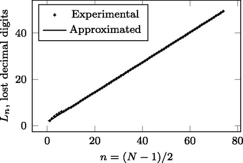The recursion defined in Theorem 3.1 involves multiplications between bounded numbers (sine and cosine always fall into $[-1,+1]$), which is beneficial from the numerical stability point of view, but subtractions are unfortunately also present, leading to a loss of precision. To overcome this loss of precision, we introduce increased precision floating point arithmetic both in our Mathematica and C++ implementations¹.^[9,10] Mathematica can quantify the precision loss, enabling us to investigate this issue experimentally. According to Figure 1, the number of accurate decimal digits lost when evaluating the SCV from the $\omega ,{\varphi }_i$ parameters (computed by the Precision function of Mathematica), denoted by L_n, is nearly linear and can be approximated by (22) $$L_n\approx 1.487+0.647n.$$(22)

Figure 1. The precision loss while computing the SCV.

In the forthcoming numerical experiments we have set the floating point precision to $L_n+16$ decimal digits to obtain an accuracy of results up to 16 decimal digits, and this precision setting eliminated all numerical issues.

It is important to note that the high precision is needed only to calculate the $a_k^{(n)},b_k^{(n)},c^{(n)}$ coefficients and the SCV itself. Representing parameters $\omega ,{\varphi }_i,i\in \{1,\dots ,n\}$ themselves does not need extra precision, and the resulting exponential cosine-square function $f^{+}(t)$ can be evaluated with machine precision as well (in the range of our interest, $n\le 1000$).

A basic pseudo-code of the computation of the SCV with the indications where high precision is needed is provided by Algorithm 1.

Algorithm 1.

Pseudo-code for the computation of the SCV

1. procedure ComputeSCV($n,\omega ,{\varphi }_i,i\in \{1,\dots ,n\}$)

2. Compute the required precision, L_n, from (22)(22) $$L_n\approx 1.487+0.647n.$$(22)

3. Convert $\omega ,{\varphi }_i,i\in \{1,\dots ,n\}$ to $L_n+16$ digits precision

4. Calculate $a_k^{(n)},b_k^{(n)},k\in \{1,\dots ,n\},c^{(n)}$ by Theorem 3.1 (high precision)

5. Calculate moments ${\mu }_0,{\mu }_1,{\mu }_2$ according to (13)(13) $$\begin{array}{c}{\mu }_0=c^{(n)}+\sum _{k=1}^n\frac{a_k^{(n)}+b_k^{(n)}k\omega }{1+{(k\omega )}^2},\\ {\mu }_1=c^{(n)}+\sum _{k=1}^n\frac{a_k^{(n)}+2b_k^{(n)}k\omega -a_k^{(n)}{(k\omega )}^2}{{(1+{(k\omega )}^2)}^2},\\ {\mu }_2=2c^{(n)}+\sum _{k=1}^n\frac{2a_k^{(n)}+6b_k^{(n)}k\omega -6a_k^{(n)}{(k\omega )}^2-2b_k^{(n)}{(k\omega )}^3}{{(1+{(k\omega )}^2)}^3}.\end{array}$$(13) (machine precision)

6. Calculate $\mathit{SCV}=\frac{{\mu }_0{\mu }_2}{{\mu }_1^2}-1$ (machine precision)

7. return SCV

8. end procedure

4. Minimizing the squared coefficient of variation

Given the size of the representation $N=2n+1,$ the $f^{+}(t)$ function providing the minimal SCV is obtained by minimizing (3)(3) $$\mathit{SCV}(f(t))=\frac{{\mu }_0{\mu }_2}{{\mu }_1^2}-1,$$(3) subject to ω and ${\varphi }_i,i\in \{1,\dots ,n\}.$ The form of the SCV does not allow a symbolic solution, and its numerical optimization is challenging, too. The surface to optimize has many local optima, hence simple gradient descent procedures failed to find the global optimum and are sensitive to the initial guess.

4.1. Optimizing the parameters

In the numerical optimization of the parameters, we had success with evolutionary optimization methods, in particular with evolution strategies. The results introduced in Horváth et al.^[7] were obtained by one of the simplest evolution strategies, the Rechenberg method.^[11]. In Horváth et al.,^[7] it was the high computational demand of the numerical integration needed to obtain the SCV and its reduced accuracy that prevented the optimization for N > 47 (n > 23).

However, computing the SCV based on the hyper-trigonometric representation using the results of Section 3.1 allows us to evaluate the moments orders of magnitudes faster and more accurately, enabling the optimization for higher n values. With the Rechenberg method (Rechenberg^[11], also referred to as (1 + 1)-ES in the literature) it is possible to obtain low SCV values relatively quickly for orders as high as n = 125, but these values are suboptimal in the majority of cases.

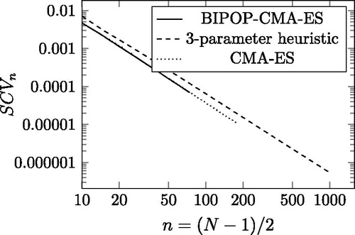
With more advanced evolution strategies the optimal SCV can be approached better. Our implementation^[9] supports the covariance matrix adoption evolution strategy (CMA-ES^[5]), and one of its variants, the BIPOP-CMA-ES with restarts.^[6]. Starting from a random initial guess, we got very low SCV values much quicker with the CMA-ES than with the (1 + 1)-ES with similar suboptimal minimum values (cf. Figure 2). The limit of applicability of CMA-ES is about n = 180. The best solution (lowest SCV for the given order), however, was always provided by the BIPOP-CMA-ES method, although it was by far the slowest among the three methods we studied. In fact, we believe that BIPOP-CMA-ES returned the global optimum for $n\in \{1,\dots ,74\},$ and we investigate the properties of those solutions in the next sections. For n > 74, we can still compute low SCV functions with the BIPOP-CMA-ES method, but its computation time gets to be prohibitive, and we are less confident about the global minimality of the results.

Figure 2. The minimal and the heuristic SCV as a function of order n in log-log scale.

For our particular problem, the running time, T, and the quality of the minimum, Q (how low the SCV is), obtained by the different optimization methods can be summarized as follows $$\begin{array}{l}{T}_{\text{CMA}-\text{ES}}< T_{(1+1)-\text{ES}}\ll T_{\text{BIPOP}-\text{CMA}-\text{ES}},\\ Q_{\text{CMA}-\text{ES}}\sim Q_{(1+1)-\text{ES}}<Q_{\text{BIPOP}-\text{CMA}-\text{ES}}.\end{array}$$

4.2. Properties of the minimal SCV solutions

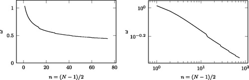
The minimal SCV values obtained by the BIPOP-CMA-ES optimization, which we conjecture to be optimal for $n\in \{1,\dots ,74\},$ are depicted in Figure 3. Apart from the minimal SCV values of the exponential cosine-square functions, Figure 3 also plots $1/(2n+1)$ and $2/{(2n+1)}^2,$ for comparison. The $\mathit{SCV}=1/N=1/(2n+1)$ is known to be the minimal SCV value for PH distributions of order N,^[1] which form a subset in the set of order N ME distributions.^[2] The $2/N^2=2/{(2n+1)}^2$ curve is reported to be the approximate decay rate in Horváth^[7], up to n = 23 (N = 47).

Figure 3. The minimal SCV of the exponential cosine-square functions as the function of n in log-log scale.

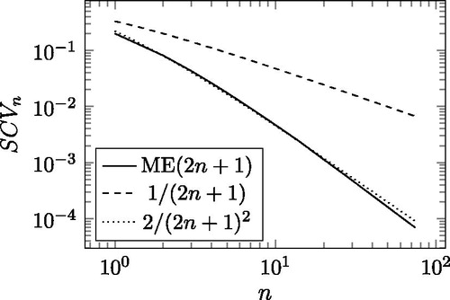
Figure 3 indicates that the SCV decreases much faster than $1/N$ and a bit faster than $2/N^2.$ Indeed, $2/N^2$ is a good approximation up to n = 23, but the decay seems to decrease below $2/N^2$ for n > 23.

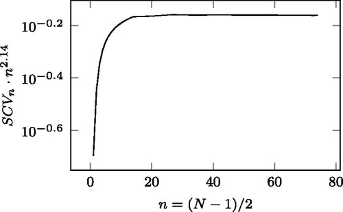
We suspect that the decrease is asymptotically polynomial (at $n\to \infty$), that we checked by plotting the $\mathit{SCV}{n}^{2.14}$ function in Figure 4. While the exponent is determined empirically and might be slightly off, it is visible that the convergence is faster than $1/n^2$ for the examined range (n < 1000).

Figure 4. The function $S(n)=SC{V}_n·n^{2.14}$ with logarithmic y axis.

4.3. The parameters providing the minimal SCV

In this section, we investigate the parameters corresponding to the minimal SCV and provide an intuitive explanation for the observed behavior. Figure 5 depicts the optimal ω parameter as a function of n. It shows a slow decrease with some inhomogeneity around $n\in \{14,28,43,60\}.$ Figure 5 suggests that ω tends to 0 as $n\to 0,$ and the inhomogeneity is related to the behavior of the ${\varphi }_k$ parameters, as it is detailed below.

Figure 5. The ω parameter providing the minimal SCV in lin-lin and log-log scales.

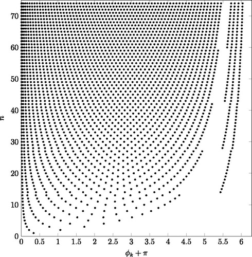
The visual appearance of the optimal ${\varphi }_k$ parameters in Figure 6 reveals many more interesting properties. First, since the period of the cosine-square function is π, the ${\varphi }_k$ parameters in (5)(5) $$f^{+}(t)=e^{-t}\prod _{i=1}^n{\hspace{0.17em}\text{cos}\hspace{0.17em}}^2\left(\frac{\omega t-{\varphi }_i}{2}\right),\hspace{1em}t\ge 0,$$(5) are $2\pi$ periodic. That is, adding an integer times $2\pi$ to any of the ${\varphi }_k$ parameters does not change the $f^{+}(t)$ function. In Figure 6 we transformed all ${\varphi }_k$ parameters to the $(-\pi ,\pi )$ range and depicted ${\varphi }_k+\pi$ instead of ${\varphi }_k$ because ${\varphi }_k+\pi$ indicates the location where the cosine-square term with ${\varphi }_k$ is zero in the $(0,2\pi )$ cycle, which is the $(0,2\pi /\omega )$ interval of $f^{+}(t).$ The nth row in Figure 6 depicts n points, which are the optimal ${\varphi }_k+\pi$ values for $k=1,\dots ,n.$ In these n points of the $(0,2\pi )$ cycle $f^{+}(t)$ equals zero. In between these zeros $f^{+}(t)$ has humps.

Figure 6. The location of the ${\varphi }_k,k=1,\dots ,n$ parameters providing the minimal SCV.

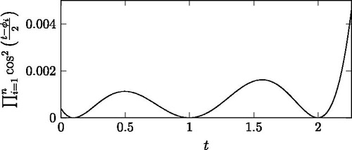
Figures 7 and 8 demonstrate the effect of ${\varphi }_k$ on $f^{+}(t)$ for ω = 1, n = 3, ${\varphi }_i+\pi \in \{0.1,1,2\}$ for $i\in \{1,2,3\}.$ In the $(0,2\pi )$ interval, both, $f^{+}(t)$ and ${\prod }_{i=1}^n{\hspace{0.17em}\text{cos}\hspace{0.17em}}^2\left(\frac{t-{\varphi }_i}{2}\right),$ have zeros at 0.1, 1 and 2. Figure 7 depicts $f^{+}(t)$ with the exponential attenuation, while Figure 8 depicts ${\prod }_{i=1}^n{\hspace{0.17em}\text{cos}\hspace{0.17em}}^2\left(\frac{t-{\varphi }_i}{2}\right)$ without the exponential attenuation. In Figure 8 the sizes of the humps depend on the distance of the neighboring zeros. The hump between 0.1 and 1 is smaller than the one between 1 and 2, which indicates that the closer the neighboring zeros are the smaller the humps are. In Figure 7, the exponential attenuation also affects the sizes of the humps. With the exponential attenuation the hump between 0.1 and 1 is larger than the one between 1 and 2. Additionally, the SCV is more sensitive to the humps further from the main peak, which motivates the fact that the ${\varphi }_k+\pi$ parameters are more concentrated around 0 to make the function as flat as possible near t = 0, where the exponential attenuation is rather weak. In Figure 7, right of the main peak, $f^{+}(t)$ is suppressed by the exponential attenuation, while left of the peak the zeros of the cosine square terms keep the function low (c.f. Figure 8).

Figure 7. $f^{+}(t)$ with ω = 1, n = 3, ${\varphi }_i+\pi \in \{0.1,1,2\}$ for $i\in \{1,2,3\}.$

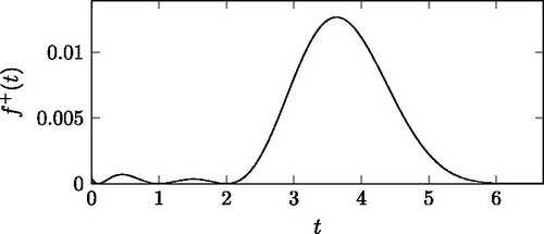
Figure 8. The initial part of ${\prod }_{i=1}^n{\hspace{0.17em}\text{cos}\hspace{0.17em}}^2\left(\frac{\omega t-{\varphi }_i}{2}\right)$ (without exponential attenuation), with ω = 1, n = 3, ${\varphi }_i+\pi \in \{0.1,1,2\}$ for $i\in \{1,2,3\}.$

In Figure 6, for n < 14, the zeros are located between 0 and 5, which means that in this range of $n f^{+}(t)$ is kept close to zero by the cosine-square functions in the interval (0, 5). It has a peak between 5 and $2\pi ,$ and the next cycles are suppressed by the exponential attenuation.

For $n\ge 14,$ there is a gap in the sequence of ${\varphi }_k$ parameters, indicating the location of a spike of $f^{+}(t).$ It means that the exponential attenuation is not strong enough for suppressing $f^{+}(t)$ right after the spike, and the minimal SCV is obtained when some cosine-square terms are used to enforce the suppression beyond the spike.

The number of cosine-square terms used to suppress $f^{+}(t)$ beyond the spike changes at $n\in \{14,28,43,60\}.$ These changes result in the small inhomogeneity in the ω values at $n\in \{14,28,43,60\}$ in Figure 5.

According to our intuitive understanding ω tends to 0 as $n\to \infty ,$ because the cosine squared terms are more efficient in suppressing $f^{+}(t)$ than the exponential attenuation, and for large n, the cosine squared terms create a sharp spike inside the $(0,2\pi )$ cycle (which is the $(0,2\pi /\omega )$ interval), such that the zeros are located on both sides of the spike. The cosine squared terms are $2\pi /\omega$ periodic and consequently, there is a spike also in the $(2\pi /\omega ,4\pi /\omega )$ interval which is suppressed by exponential attenuation. The exponential attenuation in a $2\pi /\omega$ long interval is $e^{2\pi /\omega }.$ In order to efficiently suppress the spike in the $(2\pi /\omega ,4\pi /\omega )$ interval, ω has to be small.

5. Heuristic optimization with 3 parameters

According to the previously discussed approach the number of parameters to optimize increases with n. This drawback limits the applicability of the general optimization procedures to about $n\le 74$ in the case of BIPOP-CMA-ES and about $n\le 180$ in the case of the basic CMA-ES. Using these n values the optimization procedure takes several days to terminate on an average PC clocked at 3.4 GHz.

While the $f^{+}(t)$ function obtained this way for n = 180 has an extremely low SCV ($\approx {10}^{-5}$) already, some applications might benefit from ME distributions with even lower SCV. To overcome this limitation we developed a suboptimal heuristic procedure, that aims to obtain low SCV for a given large order n.

Our heuristic procedure has to optimize only three parameters, independent of the order n. The procedure is based on the assumption that the location of the spike in the $(0,2\pi )$ cycle of the cosine-squared function plays the most important role in the SCV, and the exact values of the ${\varphi }_k$ parameters are less important, the only important feature is that the cosine-squared terms characterized by the ${\varphi }_k$ parameters should suppress $f^{+}(t)$ uniformly in the $(0,2\pi )$ cycle – apart from the spike (cf. Figure 9). In case of ME distributions, the spike is the dominant mode of the density function.

Figure 9. The spike and the zeros of $f^{+}(t).$

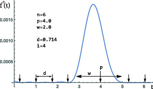
Based on this assumption we set the ${\varphi }_k$ parameters of the cosine-squared terms equidistantly. This way the position of the spike (denoted by p) and its width (w) inside the $(0,2\pi )$ interval completely define the ${\varphi }_k$ values for a given order n.

The distance of the ${\varphi }_k$ parameters (d) and the number of ${\varphi }_k$ parameters before the spike (i) can be computed from p and w by (23) $$d=\frac{2\pi -w}{n}, i=\lfloor \frac{p-w/2}{d}+\frac{1}{2}\rfloor ,$$(23) and for $k\in \{1,\dots ,n\}$ the ${\varphi }_k$ parameters are (24) $${\varphi }_k=\{\begin{array}{cc}(k-1/2)d-\pi \hfill & \text{if} k\le i,\hfill \\ (k-1/2)d+w-\pi \hfill & \text{if} k>i.\hfill \end{array}$$(24)

The obtained heuristic procedure has only 3 parameters to optimize: ω, p and w (see Algorithm 2). The SCV values computed by this heuristic optimization procedure are depicted in Figure 10 for $n\in \{10,\dots ,74\}.$ The figure indicates that for small n (n < 15) the procedure is inaccurate, but it is not a problem because the minimal SCV can be computed quickly in these cases. For larger n ($n\ge 15$) the SCV provided by the heuristic procedure is less than twice the minimal SCV in the given range. Assuming that this ratio to the optimal SCV remains valid also for n > 74 the heuristic procedure which is applicable up to n = 1000, is an efficient tool to compute highly concentrated ME distributions for large order n values.

Figure 10. The minimal and the heuristic SCV as a function of order n in log-log scale.

Algorithm 2.

The objective function of the heuristic method

1. procedure ComputeSCV-heuristic($\omega ,p,w$)

2. Obtain the distance of zeros, d, and threshold i by (23)(23) $$d=\frac{2\pi -w}{n}, i=\lfloor \frac{p-w/2}{d}+\frac{1}{2}\rfloor ,$$(23)

3. Obtain ${\varphi }_i$ for $i\in \{1,\dots ,n\}$ by (24)(24) $${\varphi }_k=\{\begin{array}{cc}(k-1/2)d-\pi \hfill & \text{if} k\le i,\hfill \\ (k-1/2)d+w-\pi \hfill & \text{if} k>i.\hfill \end{array}$$(24)

4. Compute SCV by Algorithm 1

5. return SCV

6. end procedure

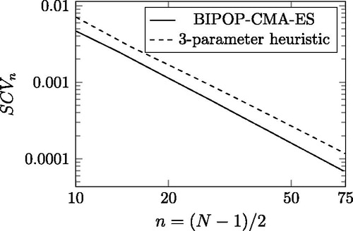
Figure 2 depicts the SCV obtained by the heuristic procedure for large n values, compared with the outputs of the highly accurate BIPOP-CMA-ES and the faster CMA-ES optimization procedures. Figure 2 suggests that the heuristic optimization remains very close to the minimum also for larger n values and the SCV obtained by the heuristic optimization maintains its polynomial decay between $n^{-2.1}$ and $n^{-2.2}.$

5.1. Implementation notes

The reader can validate the results of the paper based on the parameters we computed for a representative set of n values between 1 and 1000 and made available at https://github.com/ghorvath78/iltcme.^[10] The file itccme.json contains (among other parameters) the $a_k^{(n)},b_k^{(n)},c^{(n)}$ parameters for the computed set of n values from which $f^{+}(t)$ can be plotted using (14)(14) $$\begin{array}{cc}{f}^{+}(t)=\hfill & c^{(n)}{e}^{-t}+\frac{1}{2}\sum _{k=1}^n\left(a_k^{(n)}+\mathbb{i}{b}_k^{(n)}\right)e^{-(1+ik\omega )t}+\left(a_k^{(n)}-\mathbb{i}{b}_k^{(n)}\right)e^{-(1-ik\omega )t},\hfill \end{array}$$(14) (to check the non-negativity of $f^{+}(t)$), and the SCV can be computed using (13)(13) $$\begin{array}{c}{\mu }_0=c^{(n)}+\sum _{k=1}^n\frac{a_k^{(n)}+b_k^{(n)}k\omega }{1+{(k\omega )}^2},\\ {\mu }_1=c^{(n)}+\sum _{k=1}^n\frac{a_k^{(n)}+2b_k^{(n)}k\omega -a_k^{(n)}{(k\omega )}^2}{{(1+{(k\omega )}^2)}^2},\\ {\mu }_2=2c^{(n)}+\sum _{k=1}^n\frac{2a_k^{(n)}+6b_k^{(n)}k\omega -6a_k^{(n)}{(k\omega )}^2-2b_k^{(n)}{(k\omega )}^3}{{(1+{(k\omega )}^2)}^3}.\end{array}$$(13) in any general mathematical programing environments. Some related functions processing the parameters in itccme.json are also available at https://github.com/ghorvath78/iltcme^[10] in various programing environments. Additionally, the implementation of the optimization procedure at https://github.com/ghorvath78/cmefinder^[9] allows the reader to reproduce the parameters of the CME distributions presented in itccme.json.

The parameter setting of the code in https://github.com/ghorvath78/cmefinder^[9] resulted from the trends of the parameters depicted in Figures 5 and 6, which can also be projected to unexplored orders with some confidence. Our numerical experiments suggest that there are several local optima with similar SCV in the range of initial guesses and outside that range the obtained SCV is several orders of magnitude larger. That is, the optimization is sensitive to the initial guess, but with a proper initial guess it is insensitive to implementation details like the stopping criteria.

6. Conclusion

The paper presents a method to generate ME distributions with very low SCV. The hyper-trigonometric representation of the subset of ME distributions with exponential cosine-squared density function enables the efficient, explicit computation of the squared coefficient of variation. By selecting the appropriate numerical precision and a suitable numerical optimization method, we managed to create ME functions up to order n = 1000 with very low SCV ($<{10}^{-6}$ for n = 1000). Such non-negative, low-SCV matrix exponential functions are important ingredients in several numerical procedures, including the numerical inverse Laplace transform and representing deterministic delay in stochastic models.

Note

Additional information

Funding

This work is partially supported by the OTKA K-123914 and the TUDFO/51757/2019-ITM grants.

Notes

1 In C++ we used the mpfr library for multi-precision computations.

References

- Aldous, D.; Shepp, L. The least variable phase type distribution is Erlang. Stoch. Models 1987, 3, 467–473.
- Asmussen, S.; Bladt, M. Renewal theory and queueing algorithms for matrix-exponential distributions. In Matrix-Analytic Methods in Stochastic Models. Volume 183 of Lecture Notes in Pure and Applied Mathematics; Alfa, A. S., Chakravarthy, S. R., Eds.; New York: Marcel Dekker, 1996; pp 313–341.
- Asmussen, S.; O’Cinneide, C. A. Matrix-exponential distributions – Distributions with a rational Laplace transform. In Encyclopedia of Statistical Sciences; Kotz, S.; Read, C., Eds.; John Wiley & Sons: New York, 1997; pp 435–440.
- Éltető, T.; Rácz, S.; Telek, M. Minimal coefficient of variation of matrix exponential distributions. Presented at 2nd Madrid Conference on Queueing Theory, Madrid, Spain, Jul 2006.
- Hansen, N. The CMA evolution strategy: A comparing review. In Towards a New Evolutionary Computation; Lozano, J. A., Larrañaga, P., Inza, I., Bengoetxea, E., Eds.; Springer: Berlin, Heidelberg, 2006; pp 75–102.
- Hansen, N. Benchmarking a BI-population CMA-ES on the BBOB-2009 function testbed. Presented at Proceedings of the 11th Annual Conference Companion on Genetic and Evolutionary Computation Conference: Late Breaking Papers, ACM, Montreal, Québec, Canada, July 8–12, 2009, pp 2389–2396.
- Horváth, I.; Sáfár, O.; Telek, M.; Zámbó, B. Concentrated matrix exponential distributions. In European Workshop on Performance Engineering; Fiems, D., Paolieri, M., Platis, A. N., Eds.; Cham, Switzerland: Springer, 2016; pp 18–31.
- Horváth, I.; Talyigás, Z.; Telek, M. An optimal inverse Laplace transform method without positive and negative overshoot – An integral based interpretation. Electron. Notes Theor. Comput. Sci. 2018, 337, 87–104. DOI: 10.1016/j.entcs.2018.03.035.
- Optimization procedure for finding ME(n) with low SCV. https://github.com/ghorvath78/cmefinder [accessed Sep 22, 2019].
- Parameters of ME(n) distributions with low SCV. https://github.com/ghorvath78/iltcme [accessed Sep 22, 2019].
- Rechenberg, I. Evolutionsstrategien. In Simulationsmethoden in der Medizin und Biologie; Schneider, B., Ranft, U., Eds.; Springer-Verlag: Berlin, Heidelberg, 1978; pp 83–114.