Stochastic non-bipartite matching models and order-independent loss queues

Abstract

The problem of appropriately matching items subject to compatibility constraints arises in a number of important applications. While most of the literature on matching theory focuses on a static setting with a fixed number of items, several recent works incorporated time by considering a stochastic model in which items of different classes arrive according to independent Poisson processes and assignment constraints are described by an undirected non-bipartite graph on the classes. In this paper, we prove that the Markov process associated with this model has the same transition diagram as in a product-form queueing model called an order-independent loss queue. This allows us to adapt existing results on order-independent (loss) queues to stochastic matching models and, in particular, to derive closed-form expressions for several performance metrics, like the waiting probability or the mean matching time, that can be implemented using dynamic programming. Both these formulas and the numerical results that they allow us to derive are used to gain insight into the impact of parameters on performance. In particular, we characterize performance in a so-called heavy-traffic regime in which the number of items of a subset of the classes goes to infinity while items of other classes become scarce.

Keywords:

• Stochastic matching model
• order-independent queue
• product-form stationary distribution
• dynamic programming
• heavy-traffic regime

1. Introduction

Matching items with one another in such a way that an individual item’s preferences are met is a well-known problem in mathematics, computer science, and economics. Classical applications include assigning users to servers in distributed computing systems, joining components in assembly systems, matching passengers to drivers in ride-sharing applications, and assigning questions to experts in question-and-answer websites.

While most of the literature on matching theory focuses on a static setting in which a fixed set of items has to be matched, applications to modern large-scale service systems require that we also consider the time dimension. In assembly systems for instance, components of different types arrive at random instants as they are manufactured, and the primary objective is to have sufficient balance between components to maximize throughput while also minimizing the number of components to be stored. This observation gave rise to models that can be seen as stochastic generalizations of classical matching problems. In these stochastic matching models, items of different classes arrive according to independent Poisson processes. Compatibility constraints between items are described by an undirected graph on the classes, so that there is an edge between two classes if items of these classes can be matched with one another. In the example of Figure 1, class-3 items can be matched with items of classes 1, 2 and 4, and items of classes 1 and 2 can also be matched with one another. A matching policy is a decision rule that specifies, whenever an item arrives, to which compatible waiting unmatched item, if any, it is matched. The primary objective of a matching policy is to make the system stable in the sense that the stochastic process describing the evolution of the number of unmatched items over time is ergodic. The secondary objective is to optimize performance metrics like the mean matching time, defined as the average amount of time between the arrival of an item and its matching with another item.

Figure 1. An undirected non-bipartite compatibility graph.

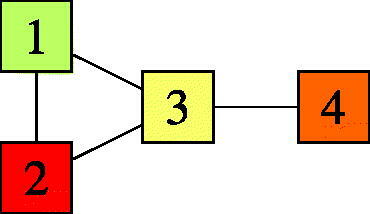
Two variants of the stochastic matching model have been studied in the literature. The stochastic bipartite matching model was introduced in Ref. [11] and further studied in Refs. [1–3, 9]. As the name suggests, this model assumes that the compatibility graph is bipartite. One can verify that such a model is always unstable if items arrive one by one at random instants (as the corresponding Markov process is either transient or null recurrent). Stability in this model is made possible by imposing that items always arrive in pairs, so that the classes of items in a pair belong to the two parts of the graph. The stochastic non-bipartite matching model, which we consider in this paper, was introduced in Ref. [20] and further studied in Refs. [4, 10, 21]. In this model, items arrive one at a time, and stability is made possible by imposing the presence of odd cycles in the compatibility graph. Mairesse and Moyal [20] consider matching policies that are admissible in the sense that the matching decision is based solely on the class of the incoming item and the sequence, in order of arrival, of classes of unmatched items. This work characterizes the maximum stability region, that is, the set of vectors of per-class arrival rates under which there exists an admissible policy that makes the system stable. The focus of Refs. [4, 10, 21] is on an admissible policy called first-come-first-matched; this is also our focus. As the name suggests, each incoming item is matched with the compatible item that has been waiting the longest, if any. In addition to being perceived as fair, this policy has the advantage of maximizing the stability region and leading to tractable results, as we will develop in this paper. The rationale behind this policy, which gives an intuition for its maximum stability, is as follows: if an item has been waiting longer than another, it is likely that this item is compatible with classes that are relatively scarcer, so that matching this item if an opportunity arises is a good heuristic to preserve stability. It is shown in Ref. [21] that this matching policy is indeed maximally stable and leads to a product-form stationary distribution. This work also derives a closed-form expression for the normalization constant of this stationary distribution. A similar closed-form expression for the mean matching time is proposed in Ref. [10], which applies this result to study the impact of the compatibility graph on performance. The authors observe that adding edges sometimes has a negative impact on performance, which is akin to Braess’s paradox in road networks. Lastly, the recent work [4] adapts some of the above results to a variant of the model in which the items of a given class can also be matched with one another.

Several recent papers [1–3, 16] have pointed out the similarity between the stationary distribution of stochastic matching models under this first-come-first-matched policy and that of order-independent queues^[5], a product-form queueing model that recently gained momentum in the queueing-theory community. Our first main contribution consists of formally proving that a stochastic non-bipartite matching model is an order-independent loss queue, a loss variant of order-independent queues introduced in Ref. [6]. This allows us to adapt known results on order-independent queues to stochastic non-bipartite matching models, and in particular to provide simpler proofs for the product-form and stability results derived in Ref. [21]. The relation with order-independent loss queues also allows us to extend these results to several variants of the model, some of which were already considered in the literature. Our second main contribution consists of closed-form expressions for several performance metrics like the waiting probability and the mean matching time. Some of these expressions can be seen as recursive variants of those derived in Refs. [10, 21], and are adapted from the works [12, 14, 22] which focus on order-independent queues and related queueing models. The recursive form of these expressions allows us to avoid duplicate calculations by using dynamic programming, which significantly reduces the complexity of the calculations. In addition to their numerical applications, these formulas allow us to gain intuition on the impact of the parameters on performance, and in particular to formalize what it means to have a balanced system. Along the same lines, our third and last contribution is a performance analysis in a scaling regime, called heavy traffic by analogy with the scaling regime of the same name in queueing theory, in which the vector of per-class arrival rates tends to a boundary of the stability region. This result can be seen as a generalization of the heavy-traffic result of Ref. [12], which focuses on order-independent queues, although the conclusion is different and illustrates the subtle difference between stochastic matching models and conventional queueing models.

The paper is organized as follows. Section 2 describes a continuous-time variant of the stochastic non-bipartite matching model proposed in Ref. [20] and introduces useful notation. In Section 3.1, we prove that this stochastic matching model is an order-independent loss queue. This result is applied in the rest of Section 3 and in Section 4 to translate known results for order-independent queues to the stochastic matching model and to generalize them. In particular, Sections 3.2 and 3.3 give simpler proofs of the product-form result and stability condition of Ref. [21], while in Section 4 we derive closed-form expressions for several performance metrics. These results are applied in Section 5 to gain insight into the impact of parameters on performance. More specifically, we propose several heuristics to minimize the mean matching time and study what happens when part of the system becomes unstable. Numerical results in Section 6 allow us to gain further insight into the dynamics of stochastic matching models. Section 7 concludes the paper.

2. Stochastic non-bipartite matching model

We first define a continuous-time variant of the stochastic non-bipartite matching model introduced in Ref. [20].

2.1. Continuous-time model

Let $\mathcal{V}=\{1,2,\dots ,N\}$ denote a finite set of item classes and consider an undirected connected non-bipartite graph without loops with vertex set $\mathcal{V}.$ This graph will be called the compatibility graph of the matching model because it will eventually describe the matching compatibilities between items. An example is shown in Figure 1. For each $i,j\in \mathcal{V},$ we write $i\sim j$ if there is an edge between classes i and j in the compatibility graph and $i\nsim j$ otherwise. For each $i\in \mathcal{V},$ we also let ${\mathcal{E}}_i\subseteq \mathcal{V}$ denote the set of neighbors of class i in the compatibility graph. With a slight abuse of notation, for each set $\mathcal{A}\subseteq \mathcal{V}$ of classes, we also let $\mathcal{E}(\mathcal{A})=\underset{i\in \mathcal{A}}{\cup }{\mathcal{E}}_i$ denote the set of classes that are neighbors of at least one class in $\mathcal{A}.$ Our assumption that the compatibility graph is non-bipartite is not necessary for the soundness of the model, but we will see in Section 3.3 that it is required for stability.

For each $i\in \mathcal{V},$ class-i items enter the system according to an independent Poisson process with rate ${\alpha }_i>0.$ As we will see in Section 3.2, we can (and will) assume without loss of generality that the vector $\alpha =({\alpha }_1,\dots ,{\alpha }_N)$ is normalized in the sense that $\sum _{i\in \mathcal{V}}{\alpha }_i=1.$ For each subset $\mathcal{A}\subseteq \mathcal{V}$ of classes, we also let $\alpha (\mathcal{A})=\sum _{i\in \mathcal{A}}{\alpha }_i$ denote the overall arrival rate of the classes in $\mathcal{A}.$ 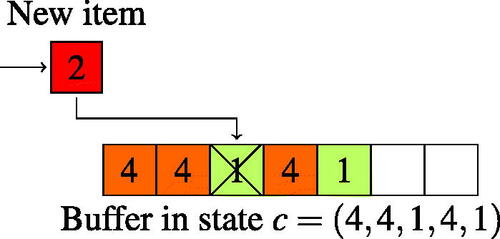All unmatched items are queued in a buffer in their arrival order. In Figure 2 for instance, unmatched items are ordered from the oldest on the left to the newest on the right, and the number written on each item represents its class. Each incoming item is matched with an item of a compatible class present in the buffer, if any, in which case both items disappear immediately; otherwise, the incoming item is added at the end of the buffer. If an incoming item finds several compatible items in the buffer, it is matched with the compatible item that has been in the buffer the longest. This matching policy is called first-come-first-matched and was studied in Refs. [4, 10, 20, 21]. Note that this matching policy can be applied with a more decentralized approach in which each item is only aware of the arrival order of its compatible items. Such a decentralized approach leads to the same dynamics and therefore to the same performance measures.

Figure 2. Unmatched items are ordered in the buffer from the oldest item on the left to the newest on the right. In particular, in the state $c=(4,4,1,4,1)$ depicted in the picture, the oldest item is of class 4 and the newest is of class 1. With the compatibility graph of Fig. 1, if a class-2 item arrives while the system is in this state, this item scans the buffer from left to right until it finds a compatible item, and is therefore matched with the oldest class-1 item. The new system state after this transition is $d=(4,4,4,1).$

2.2. Markov process

We now define a Markov process that describes the evolution of the continuous-time stochastic matching model that we have just introduced.

2.2.1. Markovian state

We describe the system state with the sequence of unmatched item classes present in the buffer. More specifically, we consider the sequence $c=(c_1,\dots ,c_n),$ where n is the number of items in the buffer and c_p is the class of the p-th oldest item, for each $p\in \{1,\dots ,n\}.$ In particular, c₁ is the class of the item that has been in the buffer the longest. Figure 2 shows a possible buffer state associated with the compatibility graph of Figure 1, with the newest items on the left. The corresponding state descriptor is $c=(4,4,1,4,1).$ We assume that the state is initially empty, with n = 0, in which case we write $c=Ø.$ The assumption that each class of items arrives according to an independent Poisson process guarantees that the stochastic process defined by the evolution of this state descriptor over time has the Markov property. When the system is in state $c=(c_1,\dots ,c_n)$ and a class-i item arrives, the new system state is $(c_1,\dots ,c_n,i)$ if $c_p\nsim i$ for each $p\in \{1,\dots ,n\}$ and $(c_1,\dots ,c_{q-1},c_{q+1},\dots ,c_n),$ where $q=\min \{p\in \{1,\dots ,n\}:c_p\sim i\},$ otherwise. The overall departure rate from each state is $\sum _{i\in \mathcal{V}}{\alpha }_i=1.$

2.2.2. State space

The system state $c=(c_1,\dots ,c_n)$ belongs to the set ${\mathcal{V}}^{*}$ made of the finite sequences over the alphabet $\mathcal{V},$ but the matching policy imposes additional restrictions on the form of this sequence. More specifically, the buffer cannot contain customers of classes $i,j\in \mathcal{V}$ such that $i\sim j,$ as the newest of the two items would necessarily have been matched with the oldest (or with an older compatible item) upon arrival. In Figure 2 for instance, an incoming class-2 item would be matched with the oldest class-1 item, so that items of classes 1 and 2 cannot be in the buffer at the same time. Therefore, in general, the state space of the Markov process defined by the system state is a strict subset of ${\mathcal{V}}^{*}$ which we denote by $\mathcal{C}.$ To better describe the structure of this state space, additional notation is introduced in the next paragraph.

A nonempty set $\mathcal{I}\subseteq \mathcal{V}$ is called an independent set (of the compatibility graph) if $i\nsim j$ for each $i,j\in \mathcal{I}.$ In other words, the set $\mathcal{I}$ is independent if the intersection of this set with the set $\mathcal{E}(\mathcal{I})$ of its neighbors is empty. The set of all independent sets is denoted by $\mathbb{I}.$ As an example, the set of independent sets of the compatibility graph of Figure 1 is $\mathbb{I}=\left\{\right\{1\},\{2\},\{3\},\{4\},\{1,4\},\{2,4\left\}\right\}.$ In general, if a set $\mathcal{I}\subseteq \mathcal{V}$ is an independent set, then any nonempty subset of $\mathcal{I}$ is also an independent set. For convenience, we also let ${\mathbb{I}}_0=\mathbb{I}\cup \{\varnothing \}$ denote the set of independent sets completed with the empty set.

For each $\mathcal{I}\in {\mathbb{I}}_0,$ we let ${\mathcal{C}}_{\mathcal{I}}$ denote the set of words in ${\mathcal{V}}^{*}$ that contain exactly the classes in $\mathcal{I}.$ Equivalently, if $\mathcal{V}(c)\subseteq \mathcal{V}$ denotes the set of item classes present in the word $c\in {\mathcal{V}}^{*},$ we have $c\in {\mathcal{C}}_{\mathcal{I}}$ if and only if $\mathcal{V}(c)=\mathcal{I}.$ Observe that ${\mathcal{C}}_{\mathcal{I}}$ is a strict subset of ${\mathcal{I}}^{*}$ in general, as words in ${\mathcal{I}}^{*}$ need not contain all classes in $\mathcal{I}.$ In the special case where $\mathcal{I}=\varnothing ,$ the set ${\mathcal{C}}_{\mathcal{I}}$ contains only the empty state $Ø.$ With this notation, the state space of the Markov process defined in the previous paragraph can be partitioned as follows: (1) $$\mathcal{C}=\underset{\mathcal{I}\in {\mathbb{I}}_0}{\cup }{\mathcal{C}}_{\mathcal{I}}.$$(1)

In particular, the set of item classes present in a feasible state of the matching model is an independent set.

Remark.

The stochastic non-bipartite matching model of Refs. [4, 10, 20, 21] works in the same way as the one presented above, except that time is slotted and there is exactly one arrival during each time slot. More specifically, the classes of incoming items during different time slots are independent and identically distributed and, for each $i\in \mathcal{V},$ α_i is the probability that an incoming item is of class i. One can verify that the (discrete-time) Markov chain associated with the state of this discrete-time stochastic matching model is the jump chain of the Markov process defined above. Since the departure rate from each state in the Markov process is $\sum _{i\in \mathcal{V}}{\alpha }_i=1,$ inspection of the balance equations reveals that the Markov chain and the Markov process have the same stationary measures. Consequently, the results in Ref. [21, Theorem 1], derived for the discrete-time stochastic matching model, also apply to the continuous-time stochastic matching model defined above. These results will be recalled in Sections 3.2 and 3.3. For simplicity, the continuous-time stochastic non-bipartite matching model introduced in Section 2.1 will be called the stochastic matching model in the remainder.

3. Product-form queueing model

In Section 3.1, we prove that the stochastic matching model of Section 2.1 is an instance of a queueing model, called an order-independent loss queue^[6], that is known to have a product-form stationary distribution. We then identify several extensions of the stochastic matching model that can also be cast as order-independent loss queues. In Sections 3.2 and 3.3, we use this observation to provide simpler proofs for two results from the literature on stochastic matching models. The reader who is more interested in understanding the long-term performance of the stochastic matching model can skip Section 3.1 and move directly to Section 3.2.

3.1. Order-independent loss queue

Our definition of order-independent loss queues, given in Definition 1 below, differs in spirit from that of Ref. [6, Section 1] in that conditions are given directly in terms of the associated Markov process, rather than in terms of the queueing system itself. In particular, although the name loss usually entails rejecting customers, here this manifests itself via the fact that the state space $\mathcal{C}$ may be a strict subset of ${\mathcal{V}}^{*}.$ This definition happens to be more convenient to show the connection with the stochastic matching model of Section 2.1, and preserves all the properties of the order-independent loss queues defined in Ref. [6]. We also make a few restrictions (such as imposing constant arrival rates) compared to Ref. [6] to avoid introducing superfluous notation.

Definition 1.

Consider a queueing system with a set $\mathcal{V}=\{1,\dots ,N\}$ of customer classes. This queueing system is called an order-independent loss queue with state space $\mathcal{C}\subseteq {\mathcal{V}}^{*},$ arrival-rate vector $\lambda =({\lambda }_1,\dots ,{\lambda }_N),$ and departure-rate function $\mu :\mathcal{C}\to {\mathbb{R}}_{+}$ if the following conditions are satisfied:

1. The evolution over time of the sequence $c=(c_1,\dots ,c_n)\in \mathcal{V}$ of classes of present customers, ordered by arrival, defines a Markov process such that:

   1. The state space of this Markov process is $\mathcal{C}.$

   2. The transitions from each state $(c_1,\dots ,c_n)\in \mathcal{C}$ are given as follows:

      • For each class $i\in \mathcal{V}$ such that $(c_1,\dots ,c_n,i)\in \mathcal{C},$ there is a transition from state c to state $(c_1,\dots ,c_n,i)$ with rate λ_i.

      • For each position $p\in \{1,\dots ,n\}$ such that $\mu (c_1,\dots ,c_p)>\mu (c_1,\dots ,c_{p-1}),$ there is a transition from state ($c_1,\dots ,c_n$) to state $(c_1,\dots ,c_{p-1},c_{p+1},\dots ,c_n)$ with rate $\mu (c_1,\dots ,c_p)-\mu (c_1,\dots ,c_{p-1})$ (with the convention that $(c_1,\dots ,c_{p-1})=Ø$ if p = 1).

2. The state space $\mathcal{C}$ satisfies the following condition:

   1. if $(c_1,\dots ,c_n)\in \mathcal{C},$ then $(c_{\sigma (1)},\dots ,c_{\sigma (n)})\in \mathcal{C}$ for each permutation σ of $\{1,\dots ,n\},$ and

   2. if $(c_1,\dots ,c_n)\in \mathcal{C}\setminus \{Ø\},$ then $(c_1,\dots ,c_{n-1})\in \mathcal{C}.$

3. The departure-rate function μ satisfies the following conditions:

   1. $\mu (c_1,\dots ,c_n)=\mu (c_{\sigma (1)},\dots ,c_{\sigma (n)})$ for each state $(c_1,\dots ,c_n)\in \mathcal{C}$ and permutation σ on $\{1,\dots ,n\},$

   2. $\mu (c_1,\dots ,c_n,i)\ge \mu (c_1,\dots ,c_n)$ for each state $(c_1,\dots ,c_n)\in \mathcal{C}$ and class $i\in \mathcal{V}$ such that $(c_1,\dots ,c_n,i)\in \mathcal{C},$

   3. $\mu (Ø)=0$ and $\mu (c_1,\dots ,c_n)>0$ for each $(c_1,\dots ,c_n)\in \mathcal{C}\setminus Ø.$

Proposition 2 below is our first main contribution. It proves that the stochastic matching model is an order-independent loss queue. Note the form of the state space $\mathcal{C}$ defined by (1)(1) $$\mathcal{C}=\underset{\mathcal{I}\in {\mathbb{I}}_0}{\cup }{\mathcal{C}}_{\mathcal{I}}.$$(1) , which differs from classic applications of loss queueing models in that the number of items of each class can be arbitrarily large when it is not zero. Once Proposition 2 is verified, applying Ref. [6, Theorem 1] suffices to prove that the stationary measures of the Markov process defined in Section 2.2 have the product form derived in Ref. [21, Theorem 1]. Both the result and its proof will be recalled in Section 3.2 for completeness.

Proposition 2.

The stochastic matching model defined in Section 2.1 is an order-independent loss queue, in the sense of Definition 1, with the state space $\mathcal{C}$ defined by (1)(1) $$\mathcal{C}=\underset{\mathcal{I}\in {\mathbb{I}}_0}{\cup }{\mathcal{C}}_{\mathcal{I}}.$$(1) , the arrival-rate vector $\lambda =\alpha =({\alpha }_1,\dots ,{\alpha }_N)$, and the departure-rate function $\mu :\mathcal{C}\to {\mathbb{R}}_{+}$ defined by $$\mu (c)=\alpha (\mathcal{E}(\mathcal{V}(c)))\hspace{1em}c\in \mathcal{C}.$$

Proof.

The details of checking the conditions of Definition 1 are left to the reader. We simply make two remarks regarding the transitions of the Markov process defined in Section 2.2. First, for each state $c=(c_1,\dots ,c_n)\in \mathcal{C}$ and class $i\in \mathcal{V},$ we have $(c_1,\dots ,c_n,i)\in \mathcal{C}$ if and only if $i\notin \mathcal{E}(\mathcal{V}(c)),$ that is, if and only if class i cannot be matched with any class present in state c. Second, if the function $\mu :\mathcal{C}\to {\mathbb{R}}_{+}$ is as defined in the proposition, then for each state $(c_1,\dots ,c_n)\in \mathcal{C}$ and position $p\in \{1,\dots ,n\},$ the difference $$\mu (c_1,\dots ,c_p)-\mu (c_1,\dots ,c_{p-1})=\alpha \left({\mathcal{E}}_{c_p}\setminus \mathcal{E}(\mathcal{V}(c_1,\dots ,c_{p-1}))\right)$$ gives the arrival rate of the classes that can be matched with class c_p but not with the classes present in $(c_1,\dots ,c_{p-1}).$ □

Remark.

The versatility of the order-independent framework allows us to generalize the stochastic matching model introduced in Section 2.1 in several directions while preserving its product-form nature. For instance, we again obtain an order-independent loss queue if items of a given class can be matched with one another. The main difference with the original model is that the state space is reduced, as the buffer can contain at most one customer of such a class at a time. We note that this extension was considered in the recent work [4], and that the proofs of Theorems 3 and 4(1) $$\mathcal{C}=\underset{\mathcal{I}\in {\mathbb{I}}_0}{\cup }{\mathcal{C}}_{\mathcal{I}}.$$(1) in Sections 3.2 and 3.3 can be adapted to provide a simpler proof of Ref. [4, Theorem 1]. Another extension, which again leads to an order-independent loss queue, consists of describing compatibilities with a directed graph (instead of an undirected graph), so that there is an edge from class i to class j if incoming class-i items can be matched with class-j items (which does not imply that incoming class-j items can be matched with class-i items). Yet another extension consists of allowing for item abandonment^[23], meaning that an item may leave the system without being matched. The stability region and product-form stationary distribution of these extensions can be characterized by following a similar approach as in the proofs of Theorems 3 and 4, or by applying known results on order-independent queues and quasi-reversible queues, a more general class of queueing models studied in Refs. [18, Chapter 3] and [13]. A last extension consists of imposing an upper bound on the number of unmatched items (either of each class or in total), or any other rejection rule that again leads to an order-independent loss queue. In this case, the stationary distribution is the restriction of that recalled in Theorem 3 to the set of reachable states (after renormalization), and no stability condition is needed.

Remark.

The usefulness of the equivalence between stochastic matching models and conventional queueing models is particularly evident under the first-come-first-matched policy, as the corresponding queueing model is known to have a product-form stationary distribution. However, this equivalence may also prove useful to transpose existing scheduling policies into matching policies, as was done in Refs. [4, 9, 20], or to adapt exact or approximate analysis methods.

3.2. Product-form stationary distribution

The Markov process defined in Section 2.2 is irreducible. Indeed, for each state $c=(c_1,\dots ,c_n)\in \mathcal{C}$ and each state $d=(d_1,\dots ,d_m)\in \mathcal{C},$ we can first go from state c to state $Ø$ via n transitions corresponding to arrivals of items compatible with the items in state c, and then from state $Ø$ to state d via m transitions corresponding to arrivals of the items present in state d. Note that the first n transitions occur with a positive probability because the compatibility graph contains no isolated node; additionally, the latter m transitions indeed lead to state d because the set of classes in d is an independent set by definition of $\mathcal{C}.$

Theorem 3 below recalls the form of the stationary measures of the Markov process defined in Section 2.2. As observed before, this theorem is analogous to Ref. [21, Theorem 1], which was stated for the discrete-time variant of the stochastic matching model. Thanks to the relation with order-independent loss queues proved in Proposition 2, we propose a simpler proof that consists of explicitly writing the (partial) balance equations of the Markov process. This proof, which is a special case of that of Ref. [6, Theorem 1], is sketched below for completeness.

Theorem 3.

The stationary measures of the Markov process associated with the system state are of the form (2) $$\pi (c_1,\dots ,c_n)=\pi (Ø)\prod _{p=1}^n\frac{{\alpha }_{c_p}}{\alpha (\mathcal{E}(\mathcal{V}(c_1,\dots ,c_p)))},\hspace{1em}(c_1,\dots ,c_n)\in \mathcal{C},$$(2) where $\pi (Ø)$ is a normalization constant. The system is stable, in the sense that this Markov process is ergodic, if and only if (3) $$\sum _{(c_1,\dots ,c_n)\in \mathcal{C}}\prod _{p=1}^n\frac{{\alpha }_{c_p}}{\alpha (\mathcal{E}(\mathcal{V}(c_1,\dots ,c_p)))}<\infty ,$$(3) in which case the stationary distribution of the Markov process is given by (2)(2) $$\pi (c_1,\dots ,c_n)=\pi (Ø)\prod _{p=1}^n\frac{{\alpha }_{c_p}}{\alpha (\mathcal{E}(\mathcal{V}(c_1,\dots ,c_p)))},\hspace{1em}(c_1,\dots ,c_n)\in \mathcal{C},$$(2) with the normalization constant (4) $$\pi (Ø)={\left(\sum _{(c_1,\dots ,c_n)\in \mathcal{C}}\prod _{p=1}^n\frac{{\alpha }_{c_p}}{\alpha (\mathcal{E}(\mathcal{V}(c_1,\dots ,c_p)))}\right)}^{-1}.$$(4)

Sketch of proof. We will prove that any measure π of the form (2)(2) $$\pi (c_1,\dots ,c_n)=\pi (Ø)\prod _{p=1}^n\frac{{\alpha }_{c_p}}{\alpha (\mathcal{E}(\mathcal{V}(c_1,\dots ,c_p)))},\hspace{1em}(c_1,\dots ,c_n)\in \mathcal{C},$$(2) satisfies the following partial balance equations in each state $c=(c_1,\dots ,c_n)\in \mathcal{C}$:

• Equalize the flow out of state c due to the arrival of an item that can be matched with a present item and the flow into state c due to the arrival of an item that cannot be matched with a present item (if $c\ne Ø$): (5) $$\pi (c)\alpha (\mathcal{E}(\mathcal{V}(c)))=\pi (c_1,\dots ,c_{n-1}){\alpha }_{c_n}.$$(5)

• Equalize the flow out of state c due to the arrival of an item of a class $i\in \mathcal{V}\setminus \mathcal{E}(\mathcal{V}(c))$ that cannot be matched with a present item and the flow into state c due to the departure of an item of this class: (6) $$\pi (c){\alpha }_i=\sum _{p=1}^{n+1}\pi (c_1,\dots ,c_{p-1},i,c_p,\dots ,c_n)\alpha ({\mathcal{E}}_i\setminus \mathcal{E}(\mathcal{V}(c_1,\dots ,c_{p-1}))),$$(6)

with the convention that $(c_1,\dots ,c_{p-1})=Ø$ if p = 1 and $(c_p,\dots ,c_n)=Ø$ if $p=n+1.$ Observe that, for each $i\in \mathcal{V}\setminus \mathcal{E}(\mathcal{V}(c))$ and $p\in \{1,\dots ,n+1\},$ state $(c_1,\dots ,c_{p-1},i,c_p,\dots ,c_n)$ belongs to $\mathcal{C}$ because the set of item classes present in this state, $\mathcal{V}(c)\cup \left\{i\right\},$ is an independent set.

Proving that a measure π satisfies (5)(5) $$\pi (c)\alpha (\mathcal{E}(\mathcal{V}(c)))=\pi (c_1,\dots ,c_{n-1}){\alpha }_{c_n}.$$(5) and (6)(6) $$\pi (c){\alpha }_i=\sum _{p=1}^{n+1}\pi (c_1,\dots ,c_{p-1},i,c_p,\dots ,c_n)\alpha ({\mathcal{E}}_i\setminus \mathcal{E}(\mathcal{V}(c_1,\dots ,c_{p-1}))),$$(6) is sufficient to prove that π is a stationary measure of the Markov process defined by the system state, as summing these partial balance equations yields the balance equations of the Markov process. We can easily verify that any measure π of the form (2)(2) $$\pi (c_1,\dots ,c_n)=\pi (Ø)\prod _{p=1}^n\frac{{\alpha }_{c_p}}{\alpha (\mathcal{E}(\mathcal{V}(c_1,\dots ,c_p)))},\hspace{1em}(c_1,\dots ,c_n)\in \mathcal{C},$$(2) satisfies (5)(5) $$\pi (c)\alpha (\mathcal{E}(\mathcal{V}(c)))=\pi (c_1,\dots ,c_{n-1}){\alpha }_{c_n}.$$(5) . That this measure also satisfies (6)(6) $$\pi (c){\alpha }_i=\sum _{p=1}^{n+1}\pi (c_1,\dots ,c_{p-1},i,c_p,\dots ,c_n)\alpha ({\mathcal{E}}_i\setminus \mathcal{E}(\mathcal{V}(c_1,\dots ,c_{p-1}))),$$(6) can be proved by induction over the buffer length n, in a similar way as in Ref. [5, Theorem 1].

The stability condition (3)(3) $$\sum _{(c_1,\dots ,c_n)\in \mathcal{C}}\prod _{p=1}^n\frac{{\alpha }_{c_p}}{\alpha (\mathcal{E}(\mathcal{V}(c_1,\dots ,c_p)))}<\infty ,$$(3) means that there exists a stationary measure whose sum is finite, which is indeed necessary and sufficient for ergodicity of the Markov process. Lastly, the constant $\pi (Ø)$ given by (4)(4) $$\pi (Ø)={\left(\sum _{(c_1,\dots ,c_n)\in \mathcal{C}}\prod _{p=1}^n\frac{{\alpha }_{c_p}}{\alpha (\mathcal{E}(\mathcal{V}(c_1,\dots ,c_p)))}\right)}^{-1}.$$(4) is chosen such that the stationary distribution sums to one. □

Multiplying all arrival rates α_i for $i\in \mathcal{V}$ by the same positive constant does not modify the form of the stationary measures (2)(2) $$\pi (c_1,\dots ,c_n)=\pi (Ø)\prod _{p=1}^n\frac{{\alpha }_{c_p}}{\alpha (\mathcal{E}(\mathcal{V}(c_1,\dots ,c_p)))},\hspace{1em}(c_1,\dots ,c_n)\in \mathcal{C},$$(2) . Indeed, this amounts to rescaling time without modifying the relative importance of the states. In particular, as already stated in Section 2.1, we can assume without loss of generality that $\sum _{i\in \mathcal{V}}{\alpha }_i=1,$ so that α_i is also the fraction of arrivals that are of class i. In the remainder, it will also be more convenient to define the stationary measures (2)(2) $$\pi (c_1,\dots ,c_n)=\pi (Ø)\prod _{p=1}^n\frac{{\alpha }_{c_p}}{\alpha (\mathcal{E}(\mathcal{V}(c_1,\dots ,c_p)))},\hspace{1em}(c_1,\dots ,c_n)\in \mathcal{C},$$(2) with the following recursion: (7) $$\pi (c_1,\dots ,c_n)=\frac{{\alpha }_{c_n}}{\alpha (\mathrm{E}(\mathrm{V}(c_1,\dots ,c_n)))}\pi (c_1,\dots ,c_{n-1}),\hspace{1em}(c_1,\dots ,c_n)\in \mathrm{C}\setminus \{Ø\}.$$(7)

3.3. Stability condition

We now recall the stability condition derived in Ref. [21, Theorem 1] and again provide a simpler proof based on the relation with order-independent loss queues.

Theorem 4.

The stochastic matching model is stable, in the sense that the associated Markov process is ergodic, if and only if (8) $$\alpha (\mathcal{I})<\alpha (\mathcal{E}(\mathcal{I})),\hspace{1em}\mathcal{I}\in \mathbb{I}.$$(8)

Sketch of proof. The proof consists of showing that (3)(3) $$\sum _{(c_1,\dots ,c_n)\in \mathcal{C}}\prod _{p=1}^n\frac{{\alpha }_{c_p}}{\alpha (\mathcal{E}(\mathcal{V}(c_1,\dots ,c_p)))}<\infty ,$$(3) is satisfied if and only if the arrival rates satisfy (8)(8) $$\alpha (\mathcal{I})<\alpha (\mathcal{E}(\mathcal{I})),\hspace{1em}\mathcal{I}\in \mathbb{I}.$$(8) . The key idea is to observe that the denominators in (3)(3) $$\sum _{(c_1,\dots ,c_n)\in \mathcal{C}}\prod _{p=1}^n\frac{{\alpha }_{c_p}}{\alpha (\mathcal{E}(\mathcal{V}(c_1,\dots ,c_p)))}<\infty ,$$(3) only depend on the set of classes in the sequence $(c_1,\dots ,c_p).$ Guided by this observation, we can define a new partition of the state space $\mathcal{C},$ that is a refinement of the partition $({\mathcal{C}}_{\mathcal{I}},\mathcal{I}\in {\mathbb{I}}_0),$ such that the restriction of the sum in (3)(3) $$\sum _{(c_1,\dots ,c_n)\in \mathcal{C}}\prod _{p=1}^n\frac{{\alpha }_{c_p}}{\alpha (\mathcal{E}(\mathcal{V}(c_1,\dots ,c_p)))}<\infty ,$$(3) to each part of this new partition can be written as a finite product of geometric series that are convergent if and only if the conditions (8)(8) $$\alpha (\mathcal{I})<\alpha (\mathcal{E}(\mathcal{I})),\hspace{1em}\mathcal{I}\in \mathbb{I}.$$(8) are satisfied. The details of the proof follow along the same lines as in the proof of Theorem 1 in the appendix of Ref. [7]. The only difference is that the set of customer classes that can be in the queue at the same time is an independent set, so that the stability condition is also restricted to independent sets. □

The stability condition (8)(8) $$\alpha (\mathcal{I})<\alpha (\mathcal{E}(\mathcal{I})),\hspace{1em}\mathcal{I}\in \mathbb{I}.$$(8) means that, for each independent set $\mathcal{I},$ there are enough items that can be matched with the classes in $\mathcal{I}$ to prevent items of these classes from building up in the buffer. As proved in Ref. [20], no matching policy can make the system stable if the arrival rates do not satisfy the stability condition (8)(8) $$\alpha (\mathcal{I})<\alpha (\mathcal{E}(\mathcal{I})),\hspace{1em}\mathcal{I}\in \mathbb{I}.$$(8) (in particular, first-come-first-matched is maximally stable). It is also shown in Ref. [20] that we would not be able to find arrival rates that satisfy this stability condition if the compatibility graph were bipartite. To better understand why the presence of odd cycles is necessary, we examine two toy examples. First consider a stochastic matching model similar to that of Section 2.1, except that the graph is bipartite and consists of only two classes connected by an edge. The stability condition (8)(8) $$\alpha (\mathcal{I})<\alpha (\mathcal{E}(\mathcal{I})),\hspace{1em}\mathcal{I}\in \mathbb{I}.$$(8) becomes ${\alpha }_1<{\alpha }_2$ and ${\alpha }_2<{\alpha }_1,$ and can therefore not be satisfied. Consistently, if we examine the associated Markov process, we obtain a two-sided infinite birth-and-death process, with transition rate α₁ in one direction and α₂ in the other, that is either transient (if ${\alpha }_1\ne {\alpha }_2$) or null recurrent (if ${\alpha }_1={\alpha }_2$), but cannot be positive recurrent. Now, if we instead consider a stochastic matching model with three classes that are all compatible, the stability condition (8)(8) $$\alpha (\mathcal{I})<\alpha (\mathcal{E}(\mathcal{I})),\hspace{1em}\mathcal{I}\in \mathbb{I}.$$(8) becomes ${\alpha }_1<{\alpha }_2+{\alpha }_3,{\alpha }_2<{\alpha }_1+{\alpha }_3,$ and ${\alpha }_3<{\alpha }_1+{\alpha }_2,$ and is satisfied for instance when ${\alpha }_1={\alpha }_2={\alpha }_3=\frac{1}{3}.$ If we examine the associated Markov process, we obtain a three-sided infinite birth-and-death process that is positive recurrent under the above conditions. In the remainder, we will assume that the stability condition (8)(8) $$\alpha (\mathcal{I})<\alpha (\mathcal{E}(\mathcal{I})),\hspace{1em}\mathcal{I}\in \mathbb{I}.$$(8) is satisfied and let π denote the stationary distribution of the Markov process.

4. Performance metrics

Another consequence of Proposition 2 is that we can adapt numerical methods originally developed for order-independent queues^{[12, 14, 22]} to stochastic matching models. Note that calculating average performance metrics associated with loss product-form queueing models is considered a hard problem in the queueing literature^[19]. Our task here is simplified by the fact that the number of items of a given class can be arbitrarily large if it is not zero, so that we can apply methods developed for open queues. Also, since we established that the continuous-time stochastic matching model and its discrete-time counterpart have the same stationary distribution, the formulas derived in this section can be applied without change to the discrete-time variant of the model.

4.1. Probability of an empty system

We first propose a new formula to compute the normalization constant of the stationary distribution of the stochastic matching model. With a slight abuse of notation, for each $\mathcal{I}\in {\mathbb{I}}_0,$ we let $\pi (\mathcal{I})$ denote the stationary probability that the set of unmatched item classes is $\mathcal{I},$ that is, (9) $$\pi (\mathcal{I})=\sum _{c\in {\mathcal{C}}_{\mathcal{I}}}\pi (c),\hspace{1em}\mathcal{I}\in {\mathbb{I}}_0.$$(9) Equation (1)(1) $$\mathcal{C}=\underset{\mathcal{I}\in {\mathbb{I}}_0}{\cup }{\mathcal{C}}_{\mathcal{I}}.$$(1) guarantees that $\sum _{\mathcal{I}\in {\mathbb{I}}_0}\pi (\mathcal{I})=1.$ The following proposition gives a recursive formula for $\pi (\mathcal{I})$ each $\mathcal{I}\in \mathbb{I}.$ We will see later that this recursive formula also gives a closed-form expression for the normalization constant $\pi (\varnothing )=\pi (Ø).$ The proof technique is similar to that of Ref. [14, Theorem 5.1], which was itself inspired from Ref. [22, Theorem 4], but the proof is more straightforward because we skip the intermediary state aggregation considered in these two works.

Proposition 5.

The stationary distribution of the set of unmatched item classes satisfies the recursion (10) $$\pi (\mathcal{I})=\frac{\sum _{i\in \mathcal{I}}{\alpha }_i\pi (\mathcal{I}\setminus \{i\})}{\alpha (\mathcal{E}(\mathcal{I}))-\alpha (\mathcal{I})},\hspace{1em}\mathcal{I}\in \mathbb{I}.$$(10)

Proof.

Let $\mathcal{I}\in \mathbb{I}.$ The proof of (10)(10) $$\pi (\mathcal{I})=\frac{\sum _{i\in \mathcal{I}}{\alpha }_i\pi (\mathcal{I}\setminus \{i\})}{\alpha (\mathcal{E}(\mathcal{I}))-\alpha (\mathcal{I})},\hspace{1em}\mathcal{I}\in \mathbb{I}.$$(10) relies on the following partition of the set ${\mathcal{C}}_{\mathcal{I}}:$ (11) $${\mathcal{C}}_{\mathcal{I}}=\underset{i\in \mathcal{I}}{\cup }\left(({\mathcal{C}}_{\mathcal{I}}·i)\cup ({\mathcal{C}}_{\mathcal{I}\setminus \left\{i\right\}}·i)\right),$$(11) where the unions are disjoint and, for each $\mathcal{D}\subseteq \mathcal{C}$ and $i\in \mathcal{V},$ we write $\mathcal{D}·i=\{(c_1,\dots ,c_n,i):(c_1,\dots ,c_n)\in \mathcal{D}\}.$ We first apply (7)(7) $$\pi (c_1,\dots ,c_n)=\frac{{\alpha }_{c_n}}{\alpha (\mathrm{E}(\mathrm{V}(c_1,\dots ,c_n)))}\pi (c_1,\dots ,c_{n-1}),\hspace{1em}(c_1,\dots ,c_n)\in \mathrm{C}\setminus \{Ø\}.$$(7) and (9)(9) $$\pi (\mathcal{I})=\sum _{c\in {\mathcal{C}}_{\mathcal{I}}}\pi (c),\hspace{1em}\mathcal{I}\in {\mathbb{I}}_0.$$(9) to rewrite $\pi (\mathcal{I})$ as follows: $$\pi (\mathcal{I})=\frac{1}{\alpha (\mathcal{E}(\mathcal{I}))}\sum _{c\in {\mathcal{C}}_{\mathcal{I}}}{\alpha }_{c_n}\pi (c_1,\dots ,c_{n-1}).$$

Then applying (11)(11) $${\mathcal{C}}_{\mathcal{I}}=\underset{i\in \mathcal{I}}{\cup }\left(({\mathcal{C}}_{\mathcal{I}}·i)\cup ({\mathcal{C}}_{\mathcal{I}\setminus \left\{i\right\}}·i)\right),$$(11) yields $$\alpha (\mathcal{E}(\mathcal{I}))\pi (\mathcal{I})=\sum _{i\in \mathcal{I}}{\alpha }_i\sum _{c\in {\mathcal{C}}_{\mathcal{I}}}\pi (c)+\sum _{i\in \mathcal{I}}{\alpha }_i\sum _{c\in {\mathcal{C}}_{\mathcal{I}\setminus \left\{i\right\}}}\pi (c),=\sum _{i\in \mathcal{I}}{\alpha }_i\pi (\mathcal{I})+\sum _{i\in \mathcal{I}}{\alpha }_i\pi (\mathcal{I}\setminus \{i\}).$$

Rearranging the terms yields (10)(10) $$\pi (\mathcal{I})=\frac{\sum _{i\in \mathcal{I}}{\alpha }_i\pi (\mathcal{I}\setminus \{i\})}{\alpha (\mathcal{E}(\mathcal{I}))-\alpha (\mathcal{I})},\hspace{1em}\mathcal{I}\in \mathbb{I}.$$(10) . □

Proposition 5 gives a closed-form expression for the normalization constant $\pi (\varnothing )=\pi (Ø).$ It suffices to observe that the unnormalized stationary measure $\psi (\mathcal{I})=\pi (\mathcal{I})/\pi (\varnothing )$ also satisfies recursion (10)(10) $$\pi (\mathcal{I})=\frac{\sum _{i\in \mathcal{I}}{\alpha }_i\pi (\mathcal{I}\setminus \{i\})}{\alpha (\mathcal{E}(\mathcal{I}))-\alpha (\mathcal{I})},\hspace{1em}\mathcal{I}\in \mathbb{I}.$$(10) . Therefore, we can first compute $\psi (\mathcal{I})$ for each $\mathcal{I}\in \mathbb{I}$ by applying recursion (10)(10) $$\pi (\mathcal{I})=\frac{\sum _{i\in \mathcal{I}}{\alpha }_i\pi (\mathcal{I}\setminus \{i\})}{\alpha (\mathcal{E}(\mathcal{I}))-\alpha (\mathcal{I})},\hspace{1em}\mathcal{I}\in \mathbb{I}.$$(10) with the base case $\psi (\varnothing )=1,$ and then derive $\pi (\varnothing )$ by normalization, that is, $\pi (\varnothing )={(\sum _{\mathcal{I}\in {\mathbb{I}}_0}\psi (\mathcal{I}))}^{-1}.$ Since there is a finite number of independent sets, this provides us with a closed-form expression for the normalization constant. Note that the denominator in (10)(10) $$\pi (\mathcal{I})=\frac{\sum _{i\in \mathcal{I}}{\alpha }_i\pi (\mathcal{I}\setminus \{i\})}{\alpha (\mathcal{E}(\mathcal{I}))-\alpha (\mathcal{I})},\hspace{1em}\mathcal{I}\in \mathbb{I}.$$(10) is always positive thanks to the stability condition (8)(8) $$\alpha (\mathcal{I})<\alpha (\mathcal{E}(\mathcal{I})),\hspace{1em}\mathcal{I}\in \mathbb{I}.$$(8) .

One can verify that unfolding the above recursion yields the closed-form expression derived in Ref. [21, Equation (5)(5) $$\pi (c)\alpha (\mathcal{E}(\mathcal{V}(c)))=\pi (c_1,\dots ,c_{n-1}){\alpha }_{c_n}.$$(5) ]. The advantage of the above recursion is that it avoids duplicate calculations. More specifically, the overall complexity to evaluate the normalization constant using (10)(10) $$\pi (\mathcal{I})=\frac{\sum _{i\in \mathcal{I}}{\alpha }_i\pi (\mathcal{I}\setminus \{i\})}{\alpha (\mathcal{E}(\mathcal{I}))-\alpha (\mathcal{I})},\hspace{1em}\mathcal{I}\in \mathbb{I}.$$(10) with dynamic programming is O(MN), where $M=\left|\mathbb{I}\right|$ is the number of independent sets and $N=\left|\mathcal{V}\right|$ is the number of item classes. By comparison, if we naively apply Ref. [21, Equation (5)(5) $$\pi (c)\alpha (\mathcal{E}(\mathcal{V}(c)))=\pi (c_1,\dots ,c_{n-1}){\alpha }_{c_n}.$$(5) ], the complexity is $O(\mathit{MNP}\times P!),$ where P is the independence number of the compatibility graph, that is, the cardinality of a maximum independent set in this graph. In both cases however, we need to enumerate all independent sets of the compatibility graph, which is an NP-hard optimization problem in general. Consequently, both formulas can be applied to make calculations only when there are few classes, when symmetries between classes can be exploited to reduce complexity (see for instance Ref. [8]), or when the graph structure guarantees that the number of independent sets is small. The same remark holds for the formulas derived in Propositions 6 to 10 below. However, we will see in Section 5 that, even when these conditions are not meet, these formulas can be used to gain insight into the impact of parameters on performance.

4.2. Waiting probability

The result of Proposition 5 gives us directly a closed-form expression for the waiting probability of the items of each class. Indeed, it follows from the PASTA property that, for each $i\in \mathcal{V},$ the waiting probability of class-i items is given by (12) $${\omega }_i=\sum _{\stackrel{\mathcal{I}\in {\mathbb{I}}_0:}{i\notin \mathcal{E}(\mathcal{I})}}\pi (\mathcal{I}).$$(12)

Upon recalling that $\sum _{i\in \mathcal{V}}{\alpha }_i=1,$ Proposition 6 below shows that the average waiting probability is simply given by $\frac{1}{2}.$ This result is not surprising. Indeed, each matching occurs between two items, one of that has just arrived (and therefore does not wait) and another that was waiting. However, this result highlights that improving the performance of one class (in terms of the waiting probability) necessarily comes at the expense of another class.

Proposition 6.

The average waiting probability is given by $\sum _{i\in \mathcal{V}}{\alpha }_i{\omega }_i=\frac{1}{2}.$

Proof.

We will verify that the per-class waiting probabilities satisfy the following conservation equation: (13) $$\sum _{i\in \mathcal{V}}{\alpha }_i{\omega }_i=\sum _{i\in \mathcal{V}}{\alpha }_i(1-{\omega }_i),$$(13) after which the result follows by rearranging the terms. We have successively: $$\sum _{i\in \mathcal{V}}{\alpha }_i(1-{\omega }_i)=\sum _{i\in \mathcal{V}}{\alpha }_i\sum _{\stackrel{\mathcal{I}\in {\mathbb{I}}_0:}{i\in \mathcal{E}(\mathcal{I})}}\pi (\mathcal{I})=\sum _{\mathcal{I}\in \mathbb{I}}\pi (\mathcal{I})\sum _{i\in \mathcal{E}(\mathcal{I})}{\alpha }_i=\sum _{\mathcal{I}\in \mathbb{I}}\pi (\mathcal{I})\alpha (\mathcal{E}(\mathcal{I})),$$ where the first equality follows from the definition of ω_i, the second by exchanging the two sums, and the third from the definition of $\alpha (\mathcal{E}(\mathcal{I})).$ Applying (10)(10) $$\pi (\mathcal{I})=\frac{\sum _{i\in \mathcal{I}}{\alpha }_i\pi (\mathcal{I}\setminus \{i\})}{\alpha (\mathcal{E}(\mathcal{I}))-\alpha (\mathcal{I})},\hspace{1em}\mathcal{I}\in \mathbb{I}.$$(10) to the last member of this equality yields $$\sum _{i\in \mathrm{V}}{\alpha }_i(1-{\omega }_i)=\sum _{\mathrm{I}\in \mathbb{I}}\left(\sum _{i\in \mathrm{I}}{\alpha }_i\pi (\mathrm{I})+\sum _{i\in \mathrm{I}}{\alpha }_i\pi (\mathrm{I}\setminus \{i\})\right),=\sum _{i\in \mathrm{V}}{\alpha }_i\sum _{\stackrel{\mathrm{I}\in {\mathbb{I}}_{\mathrm{\hspace{0.17em}}}:}{i\in \mathrm{E}(\mathrm{I})}}\left(\pi (\mathrm{I})+\pi (\mathrm{I}\setminus \{i\})\right),$$ where the second equality follows by exchanging the sums. Equation (13)(13) $$\sum _{i\in \mathcal{V}}{\alpha }_i{\omega }_i=\sum _{i\in \mathcal{V}}{\alpha }_i(1-{\omega }_i),$$(13) follows by observing that, for each $i\in \mathcal{V},$ we have $$\sum _{\stackrel{\mathcal{I}\in {\mathbb{I}}_{\mathrm{\hspace{0.17em}}}:}{i\in \mathcal{E}}}\left(\pi (\mathcal{I})+\pi (\mathcal{I}\setminus \{i\})\right)=\sum _{\stackrel{\mathcal{I}\in {\mathbb{I}}_0:}{i\notin \mathcal{E}(\mathcal{I})}}\pi (\mathcal{I})={\omega }_i,$$ where the first equality follows from a change of variable and the second by definition of ω_i. □

4.3. Mean number of unmatched items and mean matching time

Consider a random vector $X=(X_1,X_2,\dots ,X_N)$ distributed as the vector of numbers of unmatched items of each class in the stationary regime in the stochastic matching model of Section 2.1. For now, we focus on the means $L_i=\mathbb{E}\left[X_i\right]$ for each $i\in \mathcal{V},$ and we also let $L=\sum _{i\in \mathcal{V}}{L}_i$ be the mean number of unmatched items, all classes included. Propositions 7 and 8 below give a closed-form expression for these quantities by using a similar aggregation technique as in the proof of Proposition 5. As observed in Ref. [21, Section 3.4], these can be used to calculate the mean matching time of items, that is, the mean time between the arrival of an item and its matching with another item. Indeed, according to Little’s law, the mean matching time of class-i items is $L_i/{\alpha }_i,$ for each $i\in \mathcal{V},$ and the overall mean matching time is given by $L/(\sum _{i\in \mathcal{V}}{\alpha }_i)=L$ (since we assumed that $\sum _{i\in \mathcal{V}}{\alpha }_i=1$).

Proposition 7.

For each $i\in \mathcal{V}$, the mean number of unmatched class-i items is given by $$L_i=\sum _{\mathcal{I}\in \mathbb{I}:i\in \mathcal{I}}{L}_i(\mathcal{I})\pi (\mathcal{I}),$$ where $L_i(\mathcal{I})$ is the mean number of unmatched class-i items given that the set of unmatched items is $\mathcal{I}$, and is given by the recursion (14) $$L_i(\mathcal{I})\pi (\mathcal{I})=\frac{{\alpha }_i\pi (\mathcal{I})+{\alpha }_i\pi (\mathcal{I}\setminus \{i\})+\sum _{j\in \mathcal{I}\setminus \left\{i\right\}}{\alpha }_j{L}_i(\mathcal{I}\setminus \{j\})\pi (\mathcal{I}\setminus \{j\})}{\alpha (\mathcal{E}(\mathcal{I}))-\alpha (\mathcal{I})},\text{for}\text{each}\mathcal{I}\in \mathbb{I}\text{such}\text{that}i\in \mathcal{I},$$(14) with the base case $L_i(\mathcal{I})=0$ for each $\mathcal{I}\in \mathbb{I}$ such that $i\in \mathcal{I}$.

Proof.

The proof follows similar steps as that of Proposition 5, with some technical complications. Let $i\in \mathcal{V}.$ We have $L_i=\sum _{\mathcal{I}\in {\mathbb{I}}_0}{L}_i(\mathcal{I})\pi (\mathcal{I})$ where, for each $\mathcal{I}\in {\mathbb{I}}_0,L_i(\mathcal{I})$ is the mean number of unmatched class-i items given that the set of unmatched item classes is $\mathcal{I}.$ We have directly that $L_i(\mathcal{I})=0$ if $i\notin \mathcal{I}.$ If $i\in \mathcal{I},$ we have $$L_i(\mathrm{I})\pi (\mathrm{I})=\sum _{c\in {\mathrm{C}}_{\mathrm{I}}}|c{|}_i\pi (c)=\sum _{c\in {\mathrm{C}}_{\mathrm{I}}}|c{|}_i\frac{{\alpha }_{c_n}}{\alpha (\mathrm{E}(\mathrm{I}))}\pi (c_1,\dots ,c_{n-1}),$$ where $|c{|}_i$ is the number of unmatched class-i items in state c, for each $c\in \mathcal{C},$ and the second equality follows from (7)(7) $$\pi (c_1,\dots ,c_n)=\frac{{\alpha }_{c_n}}{\alpha (\mathrm{E}(\mathrm{V}(c_1,\dots ,c_n)))}\pi (c_1,\dots ,c_{n-1}),\hspace{1em}(c_1,\dots ,c_n)\in \mathrm{C}\setminus \{Ø\}.$$(7) . Applying partition (11)(11) $${\mathcal{C}}_{\mathcal{I}}=\underset{i\in \mathcal{I}}{\cup }\left(({\mathcal{C}}_{\mathcal{I}}·i)\cup ({\mathcal{C}}_{\mathcal{I}\setminus \left\{i\right\}}·i)\right),$$(11) yields $$\alpha (\mathcal{E}(\mathcal{I}))L_i(\mathcal{I})\pi (\mathcal{I})\mathrm{}={\alpha }_i[\sum _{c\in {\mathcal{C}}_{\mathcal{I}}}\left(|c{|}_i+1\right)\pi (c)+\sum _{c\in {\mathcal{C}}_{\mathcal{I}\setminus \left\{i\right\}}}\left(0+1\right)\pi (c)]+\sum _{j\in \mathcal{I}\setminus \left\{i\right\}}{\alpha }_j[\sum _{c\in {\mathcal{C}}_{\mathcal{I}}}|c{|}_i\pi (c)+\sum _{c\in {\mathcal{C}}_{\mathcal{I}\setminus \left\{j\right\}}}|c{|}_i\pi (c)].$$

This, in turn, can be rewritten as $$\begin{array}{c}\alpha (\mathcal{E}(\mathcal{I}))L_i(\mathcal{I})\pi (\mathcal{I})={\alpha }_i\left[L_i(\mathcal{I})\pi (\mathcal{I})+\pi (\mathcal{I})+\pi (\mathcal{I}\setminus \{i\})\right]\\ +\sum _{j\in \mathcal{I}\setminus \left\{i\right\}}{\alpha }_j\left[L_i(\mathcal{I})\pi (\mathcal{I})+L_i(\mathcal{I}\setminus \{j\})\pi (\mathcal{I}\setminus \{j\})\right],\\ \begin{array}{cc}\hfill & =\alpha (\mathcal{I})L_i(\mathcal{I})\pi (\mathcal{I})+{\alpha }_i\pi (\mathcal{I})+{\alpha }_i\pi (\mathcal{I}\setminus \{i\})\hfill \\ \hfill & +\sum _{j\in \mathcal{I}\setminus \left\{i\right\}}{L}_i(\mathcal{I}\setminus \{j\})\pi (\mathcal{I}\setminus \{j\}).\hfill \end{array}\end{array}$$

Rearranging the terms yields (14)(14) $$L_i(\mathcal{I})\pi (\mathcal{I})=\frac{{\alpha }_i\pi (\mathcal{I})+{\alpha }_i\pi (\mathcal{I}\setminus \{i\})+\sum _{j\in \mathcal{I}\setminus \left\{i\right\}}{\alpha }_j{L}_i(\mathcal{I}\setminus \{j\})\pi (\mathcal{I}\setminus \{j\})}{\alpha (\mathcal{E}(\mathcal{I}))-\alpha (\mathcal{I})},\text{for}\text{each}\mathcal{I}\in \mathbb{I}\text{such}\text{that}i\in \mathcal{I},$$(14) . □

To the best of our knowledge, no previous work obtained the above formula for the stochastic matching model (either in recursive or in non-recursive form). We now provide an analogous formula to directly calculate the mean number of unmatched items, all classes included, without needing to calculate the mean number of unmatched items of each class.

Proposition 8.

The mean number of unmatched items is given by $$L=\sum _{\mathcal{I}\in \mathbb{I}}L(\mathcal{I})\pi (\mathcal{I}),$$ where $L(\mathcal{I})$ is the mean number of unmatched items given that the set of unmatched items is $\mathcal{I}$, and is given by the recursion (15) $$L(\mathcal{I})\pi (\mathcal{I})=\frac{\alpha (\mathcal{E}(\mathcal{I}))\pi (\mathcal{I})+\sum _{i\in \mathcal{I}}{\alpha }_{i}L(\mathcal{I}\setminus \{i\})\pi (\mathcal{I}\setminus \{i\})}{\alpha (\mathcal{E}(\mathcal{I}))-\alpha (\mathcal{I})},\hspace{1em}\mathcal{I}\in \mathbb{I},$$(15) with the base case $L(\varnothing )=0.$

Proof.

The result follows by applying (14)(14) $$L_i(\mathcal{I})\pi (\mathcal{I})=\frac{{\alpha }_i\pi (\mathcal{I})+{\alpha }_i\pi (\mathcal{I}\setminus \{i\})+\sum _{j\in \mathcal{I}\setminus \left\{i\right\}}{\alpha }_j{L}_i(\mathcal{I}\setminus \{j\})\pi (\mathcal{I}\setminus \{j\})}{\alpha (\mathcal{E}(\mathcal{I}))-\alpha (\mathcal{I})},\text{for}\text{each}\mathcal{I}\in \mathbb{I}\text{such}\text{that}i\in \mathcal{I},$$(14) to $L(\mathcal{I})=\sum _{i\in \mathcal{I}}{L}_i(\mathcal{I})$ and simplifying the expression with (10)(10) $$\pi (\mathcal{I})=\frac{\sum _{i\in \mathcal{I}}{\alpha }_i\pi (\mathcal{I}\setminus \{i\})}{\alpha (\mathcal{E}(\mathcal{I}))-\alpha (\mathcal{I})},\hspace{1em}\mathcal{I}\in \mathbb{I}.$$(10) . □

Unfolding recursion (15)(15) $$L(\mathcal{I})\pi (\mathcal{I})=\frac{\alpha (\mathcal{E}(\mathcal{I}))\pi (\mathcal{I})+\sum _{i\in \mathcal{I}}{\alpha }_{i}L(\mathcal{I}\setminus \{i\})\pi (\mathcal{I}\setminus \{i\})}{\alpha (\mathcal{E}(\mathcal{I}))-\alpha (\mathcal{I})},\hspace{1em}\mathcal{I}\in \mathbb{I},$$(15) yields the formula given in Ref. [10, Proposition 4] but, as for the normalization constant, applying dynamic programming leads to a significant reduction of complexity compared to a naive application of this proposition. More specifically, the time complexity to compute L_i for some $i\in \mathcal{V}$ or L is O(MN) if we use our approach, while the time complexity to compute L is $O(\mathit{MNP}\times P!)$ if we naively apply the formula of Ref. [10, Proposition 4].

4.4. Distribution of the number of unmatched items

As before, let $X=(X_1,X_2,\dots ,X_N)$ be a random vector distributed like the vector of numbers of unmatched items of each class in stationary regime in the stochastic matching model of Section 2.1. A closed-form expression for the joint probability distribution of the vector X can be derived in the same way as in Ref. [14, Theorem 3.2, Equation (3.1)]. Here, we are instead interested in the probability generating function g_X of this vector, defined as (16) $$g_X(z)=\mathbb{E}\left[\prod _{i\in \mathcal{V}}{z}_i{}^{X_i}\right],\hspace{1em}z=(z_1,z_2,\dots ,z_N)\in \mathcal{Z},$$(16) where $\mathcal{Z}=\{z=(z_1,z_2,\dots ,z_N)\in {\mathbb{R}}_{+}^N:z_1\le 1,z_2\le 1,\dots ,z_N\le 1\}.$ One can show that this generating series converges whenever $z\in \mathcal{Z}.$ The following notation will be useful to state Proposition 9 below. First, for each $\lambda =({\lambda }_1,{\lambda }_2,\dots ,{\lambda }_N)\in {\mathbb{R}}_{+}^N,$ we write $\lambda (\mathcal{A})=\sum _{i\in \mathcal{A}}{\lambda }_i$ for each $\mathcal{A}\subseteq \mathcal{V}.$ Also, given two vectors $\lambda =({\lambda }_1,{\lambda }_2,\dots ,{\lambda }_N)\in {\mathbb{R}}_{+}^N$ and $\mu =({\mu }_1,{\mu }_2,\dots ,{\mu }_N)\in {\mathbb{R}}_{+}^N,$ we let $\lambda \mu =({\lambda }_1{\mu }_1,{\lambda }_2{\mu }_2,\dots ,{\lambda }_N{\mu }_N)$ denote their elementwise product. We are now in position to give a closed-form expression for the probability generating function of the vector X. Both this result and its proof are adapted from Ref. [12, Proposition 3.1].

Proposition 9.

The probability generating function of the numbers of unmatched items of each class in the buffer is given by (17) $$g_X(z)=\frac{\sum _{\mathcal{I}\in {\mathbb{I}}_0}{\psi }_{\alpha z,\alpha }(\mathcal{I})}{\sum _{\mathcal{I}\in {\mathbb{I}}_0}{\psi }_{\alpha ,\alpha }(\mathcal{I})},$$(17) where, for each $\lambda =({\lambda }_1,{\lambda }_2,\dots ,{\lambda }_N)\in {\mathbb{R}}_{+}^N$ and $\mu =({\mu }_1,{\mu }_2,\dots ,{\mu }_N)\in {\mathbb{R}}_{+}^N$ such that $\lambda (\mathcal{I})<\mu (\mathcal{E}(\mathcal{I}))$ for each $\mathcal{I}\in \mathbb{I}$, the set function ${\psi }_{\lambda ,\mu }$ is defined by the recursion (18) $${\psi }_{\lambda ,\mu }(\mathcal{I})=\frac{\sum _{i\in \mathcal{I}}{\lambda }_i{\psi }_{\lambda ,\mu }(\mathcal{I}\setminus \{i\})}{\mu (\mathcal{E}(\mathcal{I}))-\lambda (\mathcal{I})},\hspace{1em}\mathcal{I}\in \mathbb{I},$$(18) with the base case ${\psi }_{\lambda ,\mu }(\varnothing )=1.$

Proof.

It suffices to observe that, according to (2)(2) $$\pi (c_1,\dots ,c_n)=\pi (Ø)\prod _{p=1}^n\frac{{\alpha }_{c_p}}{\alpha (\mathcal{E}(\mathcal{V}(c_1,\dots ,c_p)))},\hspace{1em}(c_1,\dots ,c_n)\in \mathcal{C},$$(2) , (4)(4) $$\pi (Ø)={\left(\sum _{(c_1,\dots ,c_n)\in \mathcal{C}}\prod _{p=1}^n\frac{{\alpha }_{c_p}}{\alpha (\mathcal{E}(\mathcal{V}(c_1,\dots ,c_p)))}\right)}^{-1}.$$(4) , and (16)(16) $$g_X(z)=\mathbb{E}\left[\prod _{i\in \mathcal{V}}{z}_i{}^{X_i}\right],\hspace{1em}z=(z_1,z_2,\dots ,z_N)\in \mathcal{Z},$$(16) , $g_X(z)$ can be rewritten as $$g_X(z)=\frac{\sum _{c\in \mathcal{C}}{\prod }_{p=1}^n\frac{z_{c_p}{\alpha }_{c_p}}{\alpha (\mathcal{E}(\mathcal{V}(c_1,\dots ,c_p)))}}{\sum _{c\in \mathcal{C}}{\prod }_{p=1}^n\frac{{\alpha }_{c_p}}{\alpha (\mathcal{E}(\mathcal{V}(c_1,\dots ,c_p)))}}=\frac{\sum _{\mathcal{I}\in {\mathbb{I}}_0}\sum _{c\in {\mathcal{C}}_{\mathcal{I}}}{\prod }_{p=1}^n\frac{z_{c_p}{\alpha }_{c_p}}{\alpha (\mathcal{E}(\mathcal{V}(c_1,\dots ,c_p)))}}{\sum _{\mathcal{I}\in {\mathbb{I}}_0}\sum _{c\in {\mathcal{C}}_{\mathcal{I}}}{\prod }_{p=1}^n\frac{{\alpha }_{c_p}}{\alpha (\mathcal{E}(\mathcal{V}(c_1,\dots ,c_p)))}},=\frac{\sum _{\mathcal{I}\in {\mathbb{I}}_0}{\psi }_{z\alpha ,\alpha }(\mathcal{I})}{\sum _{\mathcal{I}\in {\mathbb{I}}_0}{\psi }_{\alpha ,\alpha }(\mathcal{I})},$$

where, for each $\lambda =({\lambda }_1,\dots ,{\lambda }_N)\in {\mathbb{R}}_{+}^N$ and $\mu =({\mu }_1,\dots ,{\mu }_N)\in {\mathbb{R}}_{+}^N$ such that $\lambda (\mathcal{I})<\mu (\mathcal{E}(\mathcal{I}))$ for each $\mathcal{I}\in \mathbb{I},$ we have $${\psi }_{\lambda ,\mu }(\mathcal{I})=\sum _{c\in {\mathcal{C}}_{\mathcal{I}}}\prod _{p=1}^n\frac{{\lambda }_{c_p}}{\mu (\mathcal{E}(\mathcal{V}(c_1,\dots ,c_p)))},\hspace{1em}\mathcal{I}\in {\mathbb{I}}_0.$$

The recursive expression (18)(18) $${\psi }_{\lambda ,\mu }(\mathcal{I})=\frac{\sum _{i\in \mathcal{I}}{\lambda }_i{\psi }_{\lambda ,\mu }(\mathcal{I}\setminus \{i\})}{\mu (\mathcal{E}(\mathcal{I}))-\lambda (\mathcal{I})},\hspace{1em}\mathcal{I}\in \mathbb{I},$$(18) follows from a similar argument as in the proof of Proposition 5. □

Taking $\lambda =\mu =\alpha$ in (18)(18) $${\psi }_{\lambda ,\mu }(\mathcal{I})=\frac{\sum _{i\in \mathcal{I}}{\lambda }_i{\psi }_{\lambda ,\mu }(\mathcal{I}\setminus \{i\})}{\mu (\mathcal{E}(\mathcal{I}))-\lambda (\mathcal{I})},\hspace{1em}\mathcal{I}\in \mathbb{I},$$(18) yields (10(10) $$\pi (\mathcal{I})=\frac{\sum _{i\in \mathcal{I}}{\alpha }_i\pi (\mathcal{I}\setminus \{i\})}{\alpha (\mathcal{E}(\mathcal{I}))-\alpha (\mathcal{I})},\hspace{1em}\mathcal{I}\in \mathbb{I}.$$(10) ), so that in particular the denominator in (17)(17) $$g_X(z)=\frac{\sum _{\mathcal{I}\in {\mathbb{I}}_0}{\psi }_{\alpha z,\alpha }(\mathcal{I})}{\sum _{\mathcal{I}\in {\mathbb{I}}_0}{\psi }_{\alpha ,\alpha }(\mathcal{I})},$$(17) is the normalization constant of the stationary distribution (2)(2) $$\pi (c_1,\dots ,c_n)=\pi (Ø)\prod _{p=1}^n\frac{{\alpha }_{c_p}}{\alpha (\mathcal{E}(\mathcal{V}(c_1,\dots ,c_p)))},\hspace{1em}(c_1,\dots ,c_n)\in \mathcal{C},$$(2) . Referring back to the order-independent loss queue introduced in Section 3.1, the vector $\lambda =({\lambda }_1,{\lambda }_2,\dots ,{\lambda }_N)$ in (18)(18) $${\psi }_{\lambda ,\mu }(\mathcal{I})=\frac{\sum _{i\in \mathcal{I}}{\lambda }_i{\psi }_{\lambda ,\mu }(\mathcal{I}\setminus \{i\})}{\mu (\mathcal{E}(\mathcal{I}))-\lambda (\mathcal{I})},\hspace{1em}\mathcal{I}\in \mathbb{I},$$(18) can be seen as the arrival rates of the customer classes, while the vector $\mu =({\mu }_1,{\mu }_2,\dots ,{\mu }_N)$ could be seen as service rates.

4.5. Distribution of the matching time

Let $T=(T_1,T_2,\dots ,T_N)$ denote a vector distributed like the vector of matching times of each class in the stationary regime in the stochastic matching model of Section 2.1. For each $i\in \mathcal{V},$ the Laplace-Stieltjes transform of the stationary matching time T_i is defined as (19) $${\phi }_{T_i}(u)=\mathbb{E}\left[e^{-u{T}_i}\right],\hspace{1em}u\in {\mathbb{R}}_{+}.$$(19)

One can show that this expectation is finite whenever $u\in {\mathbb{R}}_{+},$ but we will be especially interested in the range $0\le u\le {\alpha }_i.$ Proposition 10 below gives a closed-form expression for this Laplace-Stieltjes transform by applying the distributional form of Little’s law, in a similar way as in Ref. [12, Corollary 3.2].

Proposition 10.

For each $i\in \mathcal{V}$, the Laplace-Stieltjes transform of the matching time of class i is given by (20) $${\phi }_{T_i}(u)=g_X(z),\hspace{1em}0\le u\le {\alpha }_i,$$(20) where the function g_X is defined on $\mathcal{Z}$ by (17(17) $$g_X(z)=\frac{\sum _{\mathcal{I}\in {\mathbb{I}}_0}{\psi }_{\alpha z,\alpha }(\mathcal{I})}{\sum _{\mathcal{I}\in {\mathbb{I}}_0}{\psi }_{\alpha ,\alpha }(\mathcal{I})},$$(17) ) and the vector $z\in \mathcal{Z}$ is given by $$z_j=\{\begin{array}{cc}1-\frac{u}{{\alpha }_i}\hfill & \text{if}j=i,\hfill \\ 1\hfill & \text{if}j\in \mathcal{V}\setminus \left\{i\right\}.\hfill \end{array}$$

Proof.

Let $i\in \mathcal{V}.$ The main argument consists of observing that class i satisfies the assumptions of the following theorem, proved in Ref. [17, Theorem 1]:

Theorem 11

(Distributional form of Little’s law). Let an ergodic queueing system be such that, for a given class i of customers:

1. arrivals form a Poisson process with rate α_i;

2. all arriving customers enter the system, and remain in the system until served, i.e. there is no blocking, balking, or reneging;

3. the customers leave the system one at a time in order of arrival;

4. for any time t, the arrival process after time t and the time in the system of any customer arriving before t are independent.

Then the moment generating function $g_{X_i}$ of the ergodic number X_i of customers of this class in the system and the Laplace-Stieltjes transform ${\phi }_{T_i}$ of the ergodic time T_i spent in the system by a customer of this class satisfy $g_{X_i}(z)={\phi }_{T_i}({\alpha }_i(1-z)).$

The distributional form of Little’s law therefore implies that $${\phi }_{T_i}(u)=g_{X_i}\left(1-\frac{u}{{\alpha }_i}\right),\hspace{1em}0\le u\le {\alpha }_i,$$ where $g_{X_i}$ is the probability generating function of the stationary number X_i of unmatched class-i items. We conclude by observing that, for each $z_i\in [0,1],$ we have $g_{X_i}(z_i)=g_X(z)$ where $z\in \mathcal{Z}$ is the N-dimensional vector with z_i in component i and 1 elsewhere. □

5. Impact of load on performance

Performance in a stochastic matching model is the result of an intricate interaction between arrival rates and matching compatibilities. Even finding arrival rates that stabilize the matching model associated with a given compatibility graph is non-trivial a priori. More subtly, it was observed in Ref. [10] that, given a compatibility graph and a set of arrival rates that make the system stable, adding more edges to the compatibility graph may hurt performance (even if (8)(8) $$\alpha (\mathcal{I})<\alpha (\mathcal{E}(\mathcal{I})),\hspace{1em}\mathcal{I}\in \mathbb{I}.$$(8) guarantees that the system will remain stable). Furthermore, applying the results of Sections 3 and 4 to derive performance in a real-world matching problem will often be impossible due to the complexity of the formulas. In this section, we show that these results are also useful to gain intuition about the choices of parameters that optimize performance or at least make the system stable. By analogy with queueing theory, we define the loads of the independent sets as (21) $$\rho (\mathcal{I})=\frac{\alpha (\mathcal{I})}{\alpha (\mathcal{E}(\mathcal{I}))},\hspace{1em}\mathcal{I}\in \mathbb{I}.$$(21)

These loads will be key to analyze performance, as for instance the stability condition (8)(8) $$\alpha (\mathcal{I})<\alpha (\mathcal{E}(\mathcal{I})),\hspace{1em}\mathcal{I}\in \mathbb{I}.$$(8) can be rewritten as $\rho (\mathcal{I})<1$ for each $\mathcal{I}\in \mathbb{I}.$ Although this definition is inspired from the analogy with queueing theory, there is a fundamental difference between (21)(21) $$\rho (\mathcal{I})=\frac{\alpha (\mathcal{I})}{\alpha (\mathcal{E}(\mathcal{I}))},\hspace{1em}\mathcal{I}\in \mathbb{I}.$$(21) and the regular definition of load in a queue, namely in (21)(21) $$\rho (\mathcal{I})=\frac{\alpha (\mathcal{I})}{\alpha (\mathcal{E}(\mathcal{I}))},\hspace{1em}\mathcal{I}\in \mathbb{I}.$$(21) the arrival rates appear both in the numerator and denominator. This implies in particular that the loads are not increasing functions of the arrival rates.

5.1. Heuristics to optimize performance

Given the conclusions of Ref. [10], one may wonder, for a given vector of arrival rates $\alpha =({\alpha }_1,{\alpha }_2,\dots ,{\alpha }_N)$ and a given compatibility graph that lead to a stable stochastic matching model, whether or not removing edges from the compatibility graph may improve performance, and in this case which edge(s) should be removed. This discrete optimization problem is difficult in general, as the number of configurations is exponential in the number of classes. To gain insight into this question, we consider a related problem that consists of finding arrival rates that stabilize the system and minimize the mean matching time for a given compatibility graph. Solving this optimization problem exactly with the formulas of Section 4 is practically unfeasible when the number of classes is large, but we propose two heuristics that yield acceptable performance in practice.

5.1.1. Degree proportional

It was shown in Ref. [20, Theorem 1] that there exists a vector of arrival rates $\alpha =({\alpha }_1,{\alpha }_2,\dots ,{\alpha }_N)$ that stabilizes the system if and only if the compatibility graph is non-bipartite (which we assumed in Section 2.1), but exhibiting such arrival rates is not trivial a priori. Lemma 12 below gives a simple method to generate (an infinite number of) such arrival rates.

Lemma 12.

Let $A={(a_{i,j})}_{i,j\in \mathcal{V}}$ denote a symmetric matrix such that $a_{i,j}>0$ if and only if nodes i and j are neighbors in the compatibility graph. For each $i\in \mathcal{V}$, the weight of class i is defined as $d_i=\sum _{j\in {\mathcal{E}}_i}{a}_{i,j}$. The matching model is stable if the arrival rates are chosen to be proportional to the weights, that is, (22) $${\alpha }_i=\frac{d_i}{\sum _{j\in \mathcal{V}}{d}_j},\hspace{1em}i\in \mathcal{V}.$$(22)

Proof.

Assume that the arrival rates are given by (22)(22) $${\alpha }_i=\frac{d_i}{\sum _{j\in \mathcal{V}}{d}_j},\hspace{1em}i\in \mathcal{V}.$$(22) for some matrix A that satisfies the assumptions of the proposition, and let $d=\sum _{i\in \mathcal{V}}{d}_i.$ We will prove that these arrival rates satisfy the stability condition (8)(8) $$\alpha (\mathcal{I})<\alpha (\mathcal{E}(\mathcal{I})),\hspace{1em}\mathcal{I}\in \mathbb{I}.$$(8) . Consider an independent set $\mathcal{I}\in \mathbb{I}.$ We have successively $$d·\alpha (\mathcal{I})=\sum _{i\in \mathcal{I}}{d}_i=\sum _{i\in \mathcal{I}}\sum _{j\in {\mathcal{E}}_i}{a}_{i,j}=\sum _{j\in \mathcal{E}(\mathcal{I})}\sum _{i\in \mathcal{I}\cap {\mathcal{E}}_j}{a}_{j,i}<\sum _{j\in \mathcal{E}(\mathcal{I})}\sum _{i\in {\mathcal{E}}_j}{a}_{j,i}=\sum _{j\in \mathcal{E}(\mathcal{I})}{d}_j=d·\alpha (\mathcal{E}(\mathcal{I})).$$

To prove that the above inequality is indeed strict, it suffices to show that we cannot find an independent set $\mathcal{I}\in \mathbb{I}$ such that $\mathcal{E}(\mathcal{E}(\mathcal{I}))=\mathcal{I}.$ We can prove this by contradiction. Indeed, if there were such an independent set $\mathcal{I},$ this would imply that $\mathcal{E}(\mathcal{I})=\mathcal{V}\setminus \mathcal{I}$ (because the compatibility graph is connected) and that $\mathcal{E}(\mathcal{I})$ is also an independent set, which would contradict our assumption that the compatibility graph is non-bipartite. □

The matrix A can be interpreted as the adjacency matrix of a weighted variant of the compatibility graph. As a special case, if A is the adjacency matrix of the compatibility graph, then d_i is the degree of class i, in which case the arrival rates defined by (22)(22) $${\alpha }_i=\frac{d_i}{\sum _{j\in \mathcal{V}}{d}_j},\hspace{1em}i\in \mathcal{V}.$$(22) are called degree proportional. For example, in the graph of Figure 1, the degree-proportional arrival rates are ${\alpha }_1={\alpha }_2=\frac{1}{4},$ ${\alpha }_3=\frac{3}{8},$ and ${\alpha }_4=\frac{1}{8};$ choosing these arrival rates yields approximately a probability 0.17 that the system is empty and a mean matching time of 2.25 time units. In general, if the number of classes is sufficiently small so that all independent sets can be enumerated, this degree-proportional solution can also be used to initialize an optimization algorithm that searches for arrival rates that minimize the mean matching time by applying Proposition 8.

5.1.2. Load minimization

The loads defined in (21)(21) $$\rho (\mathcal{I})=\frac{\alpha (\mathcal{I})}{\alpha (\mathcal{E}(\mathcal{I}))},\hspace{1em}\mathcal{I}\in \mathbb{I}.$$(21) also play an instrumental role in better understanding which arrival rates yield acceptable performance. To understand this, let us first focus on the probability that the system is empty, which is the inverse of the normalization constant and is given by Proposition 5. First observe that (10)(10) $$\pi (\mathcal{I})=\frac{\sum _{i\in \mathcal{I}}{\alpha }_i\pi (\mathcal{I}\setminus \{i\})}{\alpha (\mathcal{E}(\mathcal{I}))-\alpha (\mathcal{I})},\hspace{1em}\mathcal{I}\in \mathbb{I}.$$(10) can be rewritten as (23) $$\pi (\mathcal{I})=\frac{\rho (\mathcal{I})}{1-\rho (\mathcal{I})}\left(\sum _{i\in \mathcal{I}}\frac{{\alpha }_i}{\alpha (\mathcal{I})}\pi (\mathcal{I}\setminus \{i\})\right),\hspace{1em}\mathcal{I}\in \mathbb{I},$$(23)

where the loads $\rho (\mathcal{I})$ for $\mathcal{I}\in \mathbb{I}$ are given by (21)(21) $$\rho (\mathcal{I})=\frac{\alpha (\mathcal{I})}{\alpha (\mathcal{E}(\mathcal{I}))},\hspace{1em}\mathcal{I}\in \mathbb{I}.$$(21) . Expanding the recursion yields $$\pi (\mathcal{I})=\pi (\varnothing )\sum _{s\in {\mathfrak{S}}_{\mathcal{I}}}\left(\prod _{p=1}^{\left|\mathcal{I}\right|}\frac{\rho (\{s_1,\dots ,s_p\})}{1-\rho (\{s_1,\dots ,s_p\})}\right)\left(\prod _{p=1}^{\left|\mathcal{I}\right|}\frac{{\alpha }_{s_p}}{\alpha (\{s_1,\dots ,s_p\})}\right),\hspace{1em}\mathcal{I}\in \mathbb{I},$$ where ${\mathfrak{S}}_{\mathcal{I}}$ is the set of permutations of the set $\mathcal{I},$ interpreted as the set of all sequences $s=(s_1,s_2,\dots ,s_{\left|\mathcal{I}\right|})$ in which each element of $\mathcal{I}$ appears exactly once. The first product may tend to infinity if the load $\rho (\mathcal{J})$ of any set $\mathcal{J}\subseteq \mathcal{I}$ tends to one, while the second product is always between zero and one. By applying the normalization condition, we obtain that $1/\pi (\varnothing )$ is a linear combination of products of the form $$\prod _{p=1}^n\frac{\rho (\{s_1,\dots ,s_p\})}{1-\rho (\{s_1,\dots ,s_p\})},\hspace{1em}\mathcal{I}=\{s_1,s_2,\dots ,s_n\}\in \mathbb{I}.$$

Similarly, we can rewrite (15)(15) $$L(\mathcal{I})\pi (\mathcal{I})=\frac{\alpha (\mathcal{E}(\mathcal{I}))\pi (\mathcal{I})+\sum _{i\in \mathcal{I}}{\alpha }_{i}L(\mathcal{I}\setminus \{i\})\pi (\mathcal{I}\setminus \{i\})}{\alpha (\mathcal{E}(\mathcal{I}))-\alpha (\mathcal{I})},\hspace{1em}\mathcal{I}\in \mathbb{I},$$(15) as follows: (24) $$L(\mathcal{I})\pi (\mathcal{I})=\frac{\pi (\mathcal{I})}{1-\rho (\mathcal{I})}+\frac{\rho (\mathcal{I})}{1-\rho (\mathcal{I})}\left(\sum _{i\in \mathcal{I}}\frac{{\alpha }_i}{\alpha (\mathcal{I})}L(\mathcal{I}\setminus \{i\})\pi (\mathcal{I}\setminus \{i\})\right),\hspace{1em}\hspace{1em}\mathcal{I}\in \mathbb{I}.$$(24)

In both cases, the variations of the function $x\mapsto \frac{x}{1-x}$ on (0, 1) suggest that solving the following optimization problem is a good heuristic to maximize the probability that the system is empty and minimize the mean matching time: (25) $$\begin{array}{cc}\underset{\alpha }{\text{Minimize}}\hspace{1em}\hfill & \underset{\mathcal{I}\in \mathbb{I}}{\max }\left(\rho (\mathcal{I})\right),\hfill \\ \text{subject}\mathrm{}\text{to}\hspace{1em}\hfill & {\alpha }_i\ge 0,\hspace{1em}i\in V,\hfill \\ \hfill & \sum _{i\in {\alpha }_i}{\alpha }_i=1\hfill \end{array}$$(25)

One can verify that a solution of this optimization problem satisfies the stability condition (8)(8) $$\alpha (\mathcal{I})<\alpha (\mathcal{E}(\mathcal{I})),\hspace{1em}\mathcal{I}\in \mathbb{I}.$$(8) . In the example of Figure 1, the objective function of the optimization problem (25)(25) $$\begin{array}{cc}\underset{\alpha }{\text{Minimize}}\hspace{1em}\hfill & \underset{\mathcal{I}\in \mathbb{I}}{\max }\left(\rho (\mathcal{I})\right),\hfill \\ \text{subject}\mathrm{}\text{to}\hspace{1em}\hfill & {\alpha }_i\ge 0,\hspace{1em}i\in V,\hfill \\ \hfill & \sum _{i\in {\alpha }_i}{\alpha }_i=1\hfill \end{array}$$(25) can be rewritten as $$\max \left(\frac{{\alpha }_1}{{\alpha }_2+{\alpha }_3},\frac{{\alpha }_2}{{\alpha }_1+{\alpha }_3},\frac{{\alpha }_3}{{\alpha }_1+{\alpha }_2+{\alpha }_4},\frac{{\alpha }_4}{{\alpha }_3},\frac{{\alpha }_1+{\alpha }_4}{{\alpha }_2+{\alpha }_3},\frac{{\alpha }_2+{\alpha }_4}{{\alpha }_1+{\alpha }_3}\right),$$ and the unique solution is ${\alpha }_1={\alpha }_2={\alpha }_3=\frac{1}{3}$ and ${\alpha }_4=0.$ These arrival rates happen to be a global maximum for the probability that the system is empty, with maximum value 0.25, and a local minimum for the mean matching time, with minimum value 1.5 time units¹.

In general, calculating a solution of the optimization problem (25)(25) $$\begin{array}{cc}\underset{\alpha }{\text{Minimize}}\hspace{1em}\hfill & \underset{\mathcal{I}\in \mathbb{I}}{\max }\left(\rho (\mathcal{I})\right),\hfill \\ \text{subject}\mathrm{}\text{to}\hspace{1em}\hfill & {\alpha }_i\ge 0,\hspace{1em}i\in V,\hfill \\ \hfill & \sum _{i\in {\alpha }_i}{\alpha }_i=1\hfill \end{array}$$(25) requires enumerating all independent sets, which is precisely why we may not be able to apply the results of Section 4 on the first place. This issue can be mitigated by focusing on the independent sets with cardinality at most n for some $n\ll N,$ or on the independent sets containing the most central nodes (under an appropriate definition of centrality), but the obtained solution may not be stable. To further stress the importance of minimizing the loads, we now consider a scaling regime in which the load of a (subset of) class(es) becomes close to one, thus making the system unstable.

5.3. Heavy-traffic regime

We consider a scaling regime called heavy traffic by analogy with the regime of the same name studied in queueing theory. In a nutshell, the stability condition associated with a maximal independent set becomes violated in (8)(8) $$\alpha (\mathcal{I})<\alpha (\mathcal{E}(\mathcal{I})),\hspace{1em}\mathcal{I}\in \mathbb{I}.$$(8) , so that items of these classes accumulate in the buffer (while items of other classes become scarce); our result describes the corresponding limiting distributions and performance metrics. The analysis relies on the closed-form expressions derived in Section 4. The proof technique and the results generalize those of Ref. [12, Theorem 3.1] but, as announced in the introduction, the conclusions are different and illustrate the fundamental difference between stochastic matching models and conventional queueing models.

5.3.1. Scaling regime

Fix $\mathcal{I}\in \mathbb{I},$ an independent set that is maximal with respect to the inclusion relation. We have in particular that $\mathcal{E}(\mathcal{I})=\mathcal{V}\setminus \mathcal{I}$ and $\alpha (\mathcal{I})+\alpha (\mathcal{E}(\mathcal{I}))=\alpha (\mathcal{I})+\alpha (\mathcal{V}\setminus \mathcal{I})=1.$ We consider a scaling regime where, for each $i\in \mathcal{V},$ (26) $${\alpha }_i=\{\begin{array}{cc}{p}_i\frac{\rho }{1+\rho },\hfill & i\in \mathcal{I},\hfill \\ q_i\frac{1}{1+\rho },\hfill & i\in \mathcal{V}\setminus \mathcal{I},\hfill \end{array}$$(26) with $\sum _{i\in \mathcal{I}}{p}_i=\sum _{i\in \mathcal{V}\setminus \mathcal{I}}{q}_i=1$ and $\rho \in (0,1).$ In this way, $\rho =\alpha (\mathcal{I})/\alpha (\mathcal{V}\setminus \mathcal{I})=\rho (\mathcal{I})$ is the ratio of the arrival rate of the classes in $\mathcal{I}$ to the arrival rate of their compatible classes, that is, the load of set $\mathcal{I}.$ We will show that, under some technical assumptions, as $\rho \uparrow 1,$ the buffer becomes saturated with items of the classes in $\mathcal{I}$ while running out of items of the classes in $\mathcal{V}\setminus \mathcal{I}.$ That the classes in $\mathcal{I}$ become saturated is a consequence of (26)(26) $${\alpha }_i=\{\begin{array}{cc}{p}_i\frac{\rho }{1+\rho },\hfill & i\in \mathcal{I},\hfill \\ q_i\frac{1}{1+\rho },\hfill & i\in \mathcal{V}\setminus \mathcal{I},\hfill \end{array}$$(26) , as we have (27) $$\underset{\rho \uparrow 1}{\lim }\alpha (\mathcal{I})=\underset{\rho \uparrow 1}{\lim }\alpha (\mathcal{V}\setminus \mathcal{I})=\frac{1}{2}.$$(27)

The following technical assumption guarantees that the set $\mathcal{I}$ is the only one that becomes saturated.

Assumption 13.

There exists ${\rho }^{*}\in [0,1)$ such that the stability conditions (8)(8) $$\alpha (\mathcal{I})<\alpha (\mathcal{E}(\mathcal{I})),\hspace{1em}\mathcal{I}\in \mathbb{I}.$$(8) are satisfied by the measures α defined by (26)(26) $${\alpha }_i=\{\begin{array}{cc}{p}_i\frac{\rho }{1+\rho },\hfill & i\in \mathcal{I},\hfill \\ q_i\frac{1}{1+\rho },\hfill & i\in \mathcal{V}\setminus \mathcal{I},\hfill \end{array}$$(26) for each $\rho \in ({\rho }^{*},1),$ and $$\underset{\rho \uparrow 1}{\lim }\alpha (\mathcal{J})<\underset{\rho \uparrow 1}{\lim }\alpha (\mathcal{E}(\mathcal{J})),\hspace{1em}\mathcal{J}\in \mathbb{I}\setminus \left\{\mathcal{I}\right\}.$$

5.3.2. Asymptotic distribution

Proposition 14 below shows that, under the above technical assumption, the mean number of items of the classes in $\mathcal{I}$ goes to infinity like ${(1-\rho )}^{-1}$ as $\rho \uparrow 1,$ while the mean number of items of the classes in $\mathcal{V}\setminus \mathcal{I}$ goes to zero. Furthermore, the distribution of items of the classes in $\mathcal{I}$ depends on their respective arrival rates but not on their compatibility constraints with the classes in $\mathcal{V}\setminus \mathcal{I}.$ Similarly, as intuition suggests, the waiting probability of the classes in $\mathcal{I}$ tends to one as $\rho \uparrow 1,$ while the waiting probability of the classes in $\mathcal{V}\setminus \mathcal{I}$ tends to zero. In this way, despite the structural differences between the stochastic matching model and a more conventional queueing model, the classes in $\mathcal{I}$ experience the same performance as in an M/M/1 multi-class queue in which the load ρ tends to one while, for each $i\in \mathcal{I},$ the relative arrival rate of class i is kept constant equal to p_i. The fundamental difference with an M/M/1 multi-class queue, discussed in the remark below, is that the number of items of the classes in $\mathcal{V}\setminus \mathcal{I}$ tends to zero. Given ${\rho }^{*}\in [0,1)$ and two functions f and g, defined on $({\rho }^{*},1),$ such that $g(\rho )>0$ for each $\rho \in ({\rho }^{*},1),$ we write $f(\rho )\underset{\rho \uparrow 1}{\sim }g(\rho )$ if $f(\rho )/g(\rho )\underset{\rho \uparrow 1}{\overset{}{\to }}1.$

Proposition 14.

If Assumption 13 is satisfied, then the following limiting results hold:

• (14-a) The stationary distribution of the set of unmatched item classes satisfies: $$\pi (\mathcal{I})\underset{\rho \uparrow 1}{\overset{}{\to }}1,\hspace{1em}\hspace{1em}\hspace{1em}\pi (\mathcal{J})\underset{\rho \uparrow 1}{\overset{}{\to }}0,\hspace{1em}\mathcal{J}\in {\mathbb{I}}_0\setminus \left\{\mathcal{I}\right\}.$$

• (14-b) The waiting probability of each item class satisfies: $${\omega }_i\underset{\rho \uparrow 1}{\overset{}{\to }}1,\hspace{1em}i\in \mathcal{I},\hspace{1em}\hspace{1em}{\omega }_i\underset{\rho \uparrow 1}{\overset{}{\to }}0,\hspace{1em}i\in \mathcal{V}\setminus \mathcal{I}.$$

• (14-c) The mean number of unmatched items of each class satisfies: $$L_i=\mathbb{E}\left[X_i\right]\underset{\rho \uparrow 1}{\sim }{p}_i\frac{\rho }{1-\rho },\hspace{1em}i\in \mathcal{I},\hspace{1em}\hspace{1em}{L}_i=\mathbb{E}\left[X_i\right]\underset{\rho \uparrow 1}{\overset{}{\to }}0,\hspace{1em}i\in \mathcal{V}\setminus \mathcal{I}.$$

  In particular, the limiting mean number of unmatched items (over all classes) satisfies $L\underset{\rho \uparrow 1}{\sim }\frac{\rho }{1-\rho }.$

• (14-d) The number of unmatched items of each class has the following limit in distribution: $$(1-\rho ){(X_i)}_{i\in \mathcal{I}}\underset{\rho \uparrow 1}{\overset{d}{\to }}\hspace{0.17em}\text{Exp}\hspace{0.17em}(1){(p_i)}_{i\in \mathcal{I}},\hspace{1em}\hspace{1em}{(X_i)}_{i\in \mathcal{V}\setminus \mathcal{I}}\underset{\rho \uparrow 1}{\overset{d}{\to }}0,$$

  where $\text{Exp}\hspace{0.17em}(1)$ represents a unit-mean exponentially-distributed random variable.

• (14-e) The mean matching time of each class satisfies: $$\mathbb{E}\left[T_i\right]\underset{\rho \uparrow 1}{\sim }\frac{2}{1-\rho },\hspace{1em}i\in \mathcal{I},\mathrm{}\mathrm{}\mathrm{}\mathbb{E}\left[T_i\right]\underset{\rho \uparrow 1}{\overset{}{\to }}0,\hspace{1em}i\in \mathcal{V}\setminus \mathcal{I}.$$ (14-f) The matching time of each class has the following limit in distribution: $$(1-\rho )T_i\underset{\rho \uparrow 1}{\overset{d}{\to }}\hspace{0.17em}\text{Exp}\hspace{0.17em}\left(\frac{1}{2}\right),\hspace{1em}i\in \mathcal{I},\mathrm{}\mathrm{}\mathrm{}{T}_i\underset{\rho \uparrow 1}{\overset{d}{\to }}0,\hspace{1em}i\in \mathcal{V}\setminus \mathcal{I},$$

  where $\text{Exp}\hspace{0.17em}\left(\frac{1}{2}\right)$ represents an exponentially-distributed random variable with rate $\frac{1}{2}.$

Sketch of proof. The proof of each property relies on the corresponding expression derived in Section 4. Each proof follows the same pattern: the expression for which we want to calculate the limit is a fraction whose numerator and denominator are sums of terms given by recursive expressions; we first use the recursive expressions to identify the dominating term in each sum, and then we simplify the dominating terms to derive the limit. The complete proof is given in the appendix. □

Remark.

The analysis is simplified by our choice of a maximal independent set and by Assumption 13. Indeed, these two assumptions guarantee that $\mathcal{I}$ is the only independent set that becomes saturated as $\rho \uparrow 1,$ and that all other classes are absorbed by the surplus of items in the classes in $\mathcal{I}.$ We could also consider a scaling regime where these assumptions are not satisfied. For instance, we could choose an independent set $\mathcal{I}$ that is not maximal with respect to the inclusion relation. Under some technical assumptions, we would obtain a scaling regime where the buffer becomes saturated with items of the classes in $\mathcal{I}$ and runs out of items of the classes in $\mathcal{E}(\mathcal{I}),$ while containing a positive but finite number of items of the classes in $\mathcal{V}\setminus (\mathcal{I}\cup \mathcal{E}(\mathcal{I})).$ This intermediary scaling regime becomes apparent in the numerical results of Section 6.

Remark.

The above-defined heavy-traffic regime is actually closer to a light-traffic regime for the classes in $\mathcal{V}\setminus \mathcal{I},$ as Proposition 14 shows that the number of items of these classes tends to zero. Yet, one can verify that the loads of the classes of this set do not tend to zero. These two observations may seem paradoxical, especially with conventional queueing models, like the M/M/1 queue, in mind. This apparent paradox can be explained by recalling that the arrival of an item can either increase or decrease the number of present items. This is different from conventional queueing models, in which the arrival of a customer always increases the number of present customers. Intuitively, in the scaling regime studied in this section, the arrival of an item of a class in $\mathcal{I}$ will (almost) always increase the number of unmatched items, while the arrival of an item of a class in $\mathcal{V}\setminus \mathcal{I}$ will (almost) always decrease the number of unmatched items.

6. Numerical results

In this section, we study the toy examples of Figure 3 and evaluate two performance metrics, the waiting probability and the mean matching time, defined in Sections 4.2 and 4.3. All numerical results are computed using the closed-form expressions derived in these two sections. As before, we impose that $\sum _{i\in \mathcal{V}}{\alpha }_i=1,$ so that α_i is the long-term fraction of items that belong to class i, for each $i\in \mathcal{V}.$ More specifically, in each case, we impose that ${\alpha }_2={\alpha }_3=\dots ={\alpha }_N$ and let the arrival rate α₁ of class 1 vary such that its load $\rho ={\alpha }_1/\alpha ({\mathcal{E}}_1)$ belongs to the interval (0, 1). This allows us to gain insight into the impact of varying the load of one class on performance and to illustrate the heavy-traffic result of Section 5.1.1.

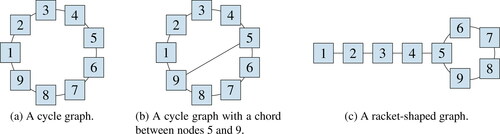
Figure 3. Toy examples with N = 9 classes.

6.1. Cycle graph

We first consider a stochastic matching model with a simple yet insightful compatibility graph, namely a cycle graph with an odd number of nodes. More specifically, we let $N=2K+1$ denote the number of classes, where $K\in \{1,2,3,\dots \},$ and we assume that, for each $i\in \mathcal{V},$ items of classes i and i + 1 can be matched with one another (with the convention that $i+1=1$ if i = N). An example of a cycle graph with N = 9 nodes is shown in Figure 3(a). The dynamics in a matching model with a cycle graph are representative of the dynamics obtained with more complex compatibility graphs. Indeed, as recalled in Section 3.3, a stochastic matching model can be stabilized if and only if its compatibility graph is non-bipartite, which means that it contains at least one odd cycle. The arrival rates are given by (28) $${\alpha }_1=\frac{\frac{\rho }{K}}{1+\frac{\rho }{K}},\hspace{1em}\hspace{1em}\hspace{1em}\hspace{1em}{\alpha }_i=\frac{\frac{1}{2K}}{1+\frac{\rho }{K}},\hspace{1em}i\in \{2,3,\dots ,N\},$$(28) so that ρ is the load of class 1. One can show by a direct reasoning² that $|\mathcal{E}(\mathcal{I})|\ge \left|\mathcal{I}\right|+1$ for each $\mathcal{I}\in \mathbb{I},$ which is sufficient to prove that, under the arrival rates (28)(28) $${\alpha }_1=\frac{\frac{\rho }{K}}{1+\frac{\rho }{K}},\hspace{1em}\hspace{1em}\hspace{1em}\hspace{1em}{\alpha }_i=\frac{\frac{1}{2K}}{1+\frac{\rho }{K}},\hspace{1em}i\in \{2,3,\dots ,N\},$$(28) , the system is stable for each $\rho \in (0,1).$ In what follows, we focus on the case N = 9 for simplicity of exposition, but the results for $N\in \{3,5,7,11,13,15\}$ (not shown here) are similar. To illustrate the performance gain permitted by the recursive expressions of Section 4 compared to existing expressions, we observe that, again with N = 9, the number of terms to sum to derive each metric is equal to 75 using dynamic programming and to 459 if we naively apply the formulas of Ref. [21, Equation (5)(5) $$\pi (c)\alpha (\mathcal{E}(\mathcal{V}(c)))=\pi (c_1,\dots ,c_{n-1}){\alpha }_{c_n}.$$(5) ] and Ref. [10, Proposition 4], giving a ratio of $459/75\simeq 6.12;$ with N = 15 classes, the numbers of terms to sum are 1,363 and 234,405, respectively, giving a ratio of $234,405/1,363\simeq 171.98.$

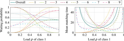
The waiting probability and mean matching time are shown in Figure 4. Because of the symmetry of the model, the performance of a class only depends on its distance to class 1, so that classes i + 1 and $N-i+1$ have the same performance for each $i\in \{1,2,\dots ,K\}.$ Focusing on the waiting probability, we can partition classes into two categories, those at an odd distance from class 1 (namely, classes 2, 4, 7, and 9) and those at an even distance from class 1 (namely, classes 1, 3, 5, 6, and 8). Indeed, as the load of class 1 increases, the waiting probability of the former set of classes decreases while that of the latter set of classes increases. The only exception is the waiting probability of classes 5 and 6, which first increases and then decreases; we will mention this again at the end of this paragraph. Intuitively, increasing the load of class 1 has the following cascading effect. To preserve the system stability, the additional class-1 items need be matched with items of classes 2 and 9, so that the waiting probability of these two classes decreases. The side effect is that there are fewer items of classes 2 and 9 to be matched with items of classes 3 and 8, so that the waiting probability of classes 3 and 8 increases. In turn, surplus items of classes 3 and 8 need be matched with items of classes 4 and 7 to preserve stability, so that the waiting probability of classes 4 and 7 decreases, and so on. The only exception is classes 5 and 6, whose waiting probability is first increasing and then decreasing. Focusing on class 5 for instance, the non-monotonic evolution of the waiting probability is the result of two conflicting effects. On the one hand, the even path 1–2–3–4–5 suggests that increasing the load of class 1 tends to increase the waiting probability of class 5. On the other hand, the odd path 1–9–8–7–6–5 suggests that increasing the load of class 1 tends to decrease the waiting probability of class 5.

Figure 4. Performance (overall and per class) in a cycle with N = 9 classes.

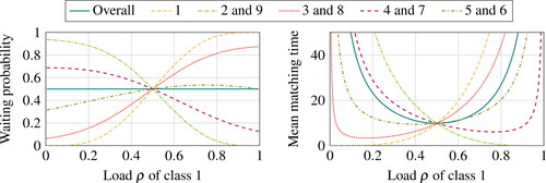
Considering the mean matching time allows us to refine the above discussion. Indeed, we can observe that, except for classes 1, 2, and 9, the mean matching time of all classes tends to infinity both when ρ tends to zero and when ρ tends to one. This suggests that not only the performance of classes 5 and 6 but also those of other classes are the result of two opposite effects, one that is conveyed by the odd-length path from class 1 and the other by the even-length path from class 1.

To better understand the speeds at which the mean matching times of classes tend to infinity, let us start with $\rho =\frac{1}{2}$ (meaning that all arrival rates are equal) and consider the chain reaction on the path 1–2–3–$\cdots$-8–9 as the load ρ decreases and tends to 1. The first class to be impacted is class 2, as this class needs the presence of class 1 to remain stable, and indeed the mean matching time of class 2 tends to infinity the fastest. The side effect is that class-3 items are matched more frequently with class-2 items, so that the mean matching time of class 3 decreases. This implies that class-3 items are less available for class 4, so that the mean matching time of class 4 is the next to tend to infinity. By repeating this reasoning, we obtain that the mean matching time of class 6 is the next to tend to infinity, followed by the mean matching time of class 8. A similar phenomenon occurs on the path 1–9–8–$\cdots$–3–2, so that the mean matching times of classes 9, 7, 5, and 3 also tend to infinity one after the other.

6.2. Cycle graph with a chord

To complement our observations, we break the model symmetry by adding a chord between classes 5 and 9. The arrival rates are still given by (28(28) $${\alpha }_1=\frac{\frac{\rho }{K}}{1+\frac{\rho }{K}},\hspace{1em}\hspace{1em}\hspace{1em}\hspace{1em}{\alpha }_i=\frac{\frac{1}{2K}}{1+\frac{\rho }{K}},\hspace{1em}i\in \{2,3,\dots ,N\},$$(28) ). It follows from (8(8) $$\alpha (\mathcal{I})<\alpha (\mathcal{E}(\mathcal{I})),\hspace{1em}\mathcal{I}\in \mathbb{I}.$$(8) ) that adding an edge to the compatibility graph cannot reduce the stability region of the corresponding stochastic matching model, so that the model is still stable for each $\rho \in (0,1).$ We again focus on a model with N = 9 classes. We have verified that the reasoning we develop below generalizes to other numbers of classes and other placements of the chord relative to class 1, although the results vary qualitatively.

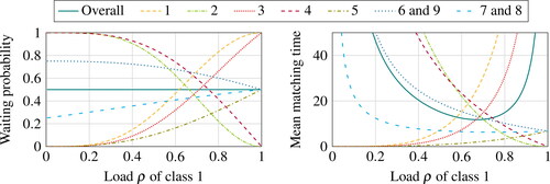
The results are shown in Figure 5. Adding a chord breaks the symmetry between classes, but we can still divide classes into several categories depending on the limiting behavior of their waiting probability and mean matching time as the load ρ tends to either zero or one. Let us first focus on the limiting regime where the load ρ tends to zero. In view of the mean matching times, the first class to become unstable is class 2, which is natural because the supply rate of class 3 items is not sufficient to maintain its stability. The main difference with the previous scenario is that the stability of class 9 is temporarily preserved by its compatibility with classes 8 and 5. The overabundance of class 2 leads to the exhaustion of class 3, which in turn leads to the overabundance of class 4, which in turn leads to the exhaustion of class 5. Once class 5 is exhausted, the next classes to become unstable are its neighbors, classes 6 and 9, which eventually leads to the overabundance of classes 7 and 8 as well. The limiting behavior as the load ρ tends to one is close to that observed for the cycle without chord. The reason is that the first immediate impact of increasing the load of class 1 is the exhaustion of class 9 (as well as class 2), rendering the presence of the chord useless, so that then we are back to the scenario of Section 6.1.

Figure 5. Performance (overall and per class) in a cycle with N = 9 classes supplemented with a chord between classes 5 and 9.

6.3. Racket-shaped graph

We finally consider the racket-shaped graph of Figure 3(c). Although a line alone cannot be stabilized because it forms a bipartite graph, this example gives us an idea of the dynamics that may arise in such a graph. One can also think of this graph as being obtained by removing the edge between nodes 1 and 9 in the cycle graph with a chord of Figure 3(b). The arrival rates of classes are given by $${\alpha }_1=\frac{\frac{\rho }{N-1}}{1+\frac{\rho }{N-1}},\hspace{1em}\hspace{1em}\hspace{1em}\hspace{1em}{\alpha }_i=\frac{\frac{1}{N-1}}{1+\frac{\rho }{N-1}},\hspace{1em}i\in \{2,3,\dots ,N\},$$ so that ρ is again the load of class 1. One can do a similar reasoning as for the cycle to show that this system is stable whenever $\rho \in (0,1).$ We again focus on a scenario with N = 9 nodes in total, 4 of which belong to the line part and 5 to the cycle part. In general, we observed that the qualitative behavior of the results depends mainly on the parity of the numbers of classes on the line part and on the circle part of the graph, and we may again adapt the reasoning below to explain this qualitative behavior.

The results for the racket-shaped graph of Figure 3(c) are shown in Figure 6. Along the line part of the graph, the impact of increasing or decreasing the load ρ of class 1 is as one could expect. For instance, as ρ tends to one, class-2 items become scarce, which leads to the instability of class 3, which in turn leads to the scarcity of class 4. Compared to the cycle with a chord, the most striking observation is that classes 5, 6, 7, 8, and 9 remain stable as the load ρ tends to one, and that these classes have the same asymptotic waiting probability and mean matching time. The reason is that, asymptotically, the model restricted to classes 5 to 9 evolves like a cycle with five classes that all have the same arrival rate, and this model is stable.

Figure 6. Performance (overall and per class) in the racket-shaped graph with N = 9 classes shown in Figure 3(c).

If we again focus on the asymptotic regime where the load ρ tends to one, it seems that the overall mean matching time is lower in the racket-shaped graph than in the cycle with a chord, which may seem counterintuitive after observing that the former is obtained by removing an edge from the latter. This observation is however consistent with the discussion of Ref. [10], which compared this phenomenon with Braess’s paradox in road networks.

7. Conclusion

In this paper, we proved that a stochastic non-bipartite matching model is an order-independent loss queue. This equivalence allowed us to propose simpler proofs for existing results and to derive new results regarding stochastic matching models. In particular, we used the order-independent queue framework to give alternative proofs for the product-form stationary distribution and the stability condition derived in Ref. [21, Theorem 1]. By adapting numerical methods developed in Ref. [12,14,22], we also derived new closed-form expressions for the normalization constant, the mean matching time, and other performance metrics. In turn, these formulas were applied to gain insight into the impact of parameters on performance. By analogy with queueing theory, we highlighted the importance of the so-called load parameters and studied the system behavior in the heavy-traffic regime, in which the load of a subset of classes becomes critical. The obtained formulas were also put in practice with numerical results.

For future works, we would like to derive simpler formulas for the performance metrics. Indeed, even though our recursive formulas allow for a dynamic-programming approach, complexity remains exponential in the number of classes in general, which limits their applicability to models with only a few classes. In parallel, we would like to understand if and how these results can be adapted to analyze the performance of stochastic matching models with a bipartite compatibility graph, like the one studied in Ref. [1–3,9,11], in which items arrive in pairs. Lastly, as mentioned before, we would like to explore the generalizations of the stochastic matching model made possible by the equivalence with order-independent loss queues. Yet another avenue for future work, which goes beyond the scope of stochastic matching models, consists of extending the heavy-traffic result proved for multi-class multi-server queues in Ref. [12] to other order-independent (loss) queues, like those considered in [14, Section 4.3].

Acknowledgement

The author is grateful to Sem Borst for his valuable comments on an earlier draft of this paper and to Ellen Cardinaels for mentioning the reference [4]. The author thanks both of them for helpful discussions on the related work [12]. The author is also grateful to the anonymous editor and reviewer for their valuable suggestions on the contents and exposition of the paper, and in particular for suggesting a simplification in Section 3.

Correction Statement

This article has been republished with minor changes. These changes do not impact the academic content of the article.

Notes

1 Although numerical evaluations suggest that this is also a global minimum, proving this conjecture is complicated by the structure of (15)(15) $$L(\mathcal{I})\pi (\mathcal{I})=\frac{\alpha (\mathcal{E}(\mathcal{I}))\pi (\mathcal{I})+\sum _{i\in \mathcal{I}}{\alpha }_{i}L(\mathcal{I}\setminus \{i\})\pi (\mathcal{I}\setminus \{i\})}{\alpha (\mathcal{E}(\mathcal{I}))-\alpha (\mathcal{I})},\hspace{1em}\mathcal{I}\in \mathbb{I},$$(15) . Better understanding the properties of the mean matching time seen as a function of the arrival rates and/or the graph structure would be an interesting topic for future work.

2 Let $\mathcal{I}\in \mathbb{I}.$ The sets $\mathcal{I}+1=\{i+1,i\in \mathcal{I}\}$ and $\mathcal{I}-1=\{i-1,i\in \mathcal{I}\}$ (again with the convention that $i+1=1$ if i = N and $i-1=N$ if $i=1$) both contain $\left|\mathcal{I}\right|$ nodes and are included into $\mathcal{E}(\mathcal{I}).$ It suffices to show that at least one of these two sets contains an element that the other does not. In turn, to prove this, it suffices to observe that an independent set $\mathcal{I}$ contains at most K nodes, so that at least two of these nodes are separated by at least two nodes that do not belong to $\mathcal{I}.$

Appendix

Proof of Proposition 14

As announced, the proof of each property relies on the corresponding expression derived in Section 4. The key argument consists of observing that Equation (27)(27) $$\underset{\rho \uparrow 1}{\lim }\alpha (\mathcal{I})=\underset{\rho \uparrow 1}{\lim }\alpha (\mathcal{V}\setminus \mathcal{I})=\frac{1}{2}.$$(27) and Assumption 13 can be reformulated as follows: as $\rho \uparrow 1,\rho (\mathcal{J})$ tends to one if $\mathcal{J}=\mathcal{I}$ (as we have $\rho (\mathcal{I})=\rho$) and to a constant strictly less than one if $\mathcal{J}\in \mathbb{I}\setminus \left\{\mathcal{I}\right\}.$

Proof of Property (14-a). According to Proposition 5 and Equation (23)(23) $$\pi (\mathcal{I})=\frac{\rho (\mathcal{I})}{1-\rho (\mathcal{I})}\left(\sum _{i\in \mathcal{I}}\frac{{\alpha }_i}{\alpha (\mathcal{I})}\pi (\mathcal{I}\setminus \{i\})\right),\hspace{1em}\mathcal{I}\in \mathbb{I},$$(23) , the stationary distribution of the set of unmatched classes can be rewritten as (29) $$\pi (\mathcal{J})=\frac{\psi (\mathcal{J})}{\sum _{\mathcal{K}\in {\mathbb{I}}_0}\psi (\mathcal{K})},\hspace{1em}\mathcal{J}\in {\mathbb{I}}_0,$$(29)

where $\psi (\mathcal{J})$ is given by $\psi (\varnothing )=1,$ and $$\psi (\mathcal{J})=\frac{\rho (\mathcal{J})}{1-\rho (\mathcal{J})}\left(\sum _{i\in \mathcal{J}}\frac{{\alpha }_i}{\alpha (\mathcal{J})}\psi (\mathcal{J}\setminus \{i\})\right),\hspace{1em}\mathcal{J}\in \mathbb{I}.$$

Since $\rho (\mathcal{J})$ tends to one if $\mathcal{J}=\mathcal{I}$ and to a constant strictly less than one if $\mathcal{J}\in \mathbb{I}\setminus \left\{\mathcal{I}\right\},$ it follows that $\psi (\mathcal{J})$ tends to infinity if $\mathcal{J}=\mathcal{I}$ and to a finite constant if $\mathcal{J}\in {\mathbb{I}}_0\setminus \left\{\mathcal{I}\right\}.$ We conclude by inserting this into (29)(29) $$\pi (\mathcal{J})=\frac{\psi (\mathcal{J})}{\sum _{\mathcal{K}\in {\mathbb{I}}_0}\psi (\mathcal{K})},\hspace{1em}\mathcal{J}\in {\mathbb{I}}_0,$$(29) . □

Proof of Property (14-b$${\omega }_i\underset{\rho \uparrow 1}{\overset{}{\to }}1,\hspace{1em}i\in \mathcal{I},\hspace{1em}\hspace{1em}{\omega }_i\underset{\rho \uparrow 1}{\overset{}{\to }}0,\hspace{1em}i\in \mathcal{V}\setminus \mathcal{I}.$$). The result for the classes in $\mathcal{I}$ follows by inserting Property (14-a) into (12(12) $${\omega }_i=\sum _{\stackrel{\mathcal{I}\in {\mathbb{I}}_0:}{i\notin \mathcal{E}(\mathcal{I})}}\pi (\mathcal{I}).$$(12) ). The result for the classes in $\mathcal{V}\setminus \mathcal{I}$ is then a consequence of (13)(13) $$\sum _{i\in \mathcal{V}}{\alpha }_i{\omega }_i=\sum _{i\in \mathcal{V}}{\alpha }_i(1-{\omega }_i),$$(13) and (27)(27) $$\underset{\rho \uparrow 1}{\lim }\alpha (\mathcal{I})=\underset{\rho \uparrow 1}{\lim }\alpha (\mathcal{V}\setminus \mathcal{I})=\frac{1}{2}.$$(27) . □

Proof of Property (14-c$$L_i=\mathbb{E}\left[X_i\right]\underset{\rho \uparrow 1}{\sim }{p}_i\frac{\rho }{1-\rho },\hspace{1em}i\in \mathcal{I},\hspace{1em}\hspace{1em}{L}_i=\mathbb{E}\left[X_i\right]\underset{\rho \uparrow 1}{\overset{}{\to }}0,\hspace{1em}i\in \mathcal{V}\setminus \mathcal{I}.$$) and (14-e$$\mathbb{E}\left[T_i\right]\underset{\rho \uparrow 1}{\sim }\frac{2}{1-\rho },\hspace{1em}i\in \mathcal{I},\mathrm{}\mathrm{}\mathrm{}\mathbb{E}\left[T_i\right]\underset{\rho \uparrow 1}{\overset{}{\to }}0,\hspace{1em}i\in \mathcal{V}\setminus \mathcal{I}.$$). Consider a class $i\in \mathcal{I}.$ According to Proposition 7 and Equation (29)(29) $$\pi (\mathcal{J})=\frac{\psi (\mathcal{J})}{\sum _{\mathcal{K}\in {\mathbb{I}}_0}\psi (\mathcal{K})},\hspace{1em}\mathcal{J}\in {\mathbb{I}}_0,$$(29) , the expected number of class-i items can be rewritten as (30) $$L_i=\frac{\sum _{\mathcal{J}\in {\mathbb{I}}_0:i\in \mathcal{J}}{L}_i(\mathcal{J})\psi (\mathcal{J})}{\sum _{\mathcal{J}\in {\mathbb{I}}_0}\psi (\mathcal{J})},$$(30) where $L_i(\mathcal{J})\psi (\mathcal{J})$ is given by $L_i(\mathcal{J})\psi (\mathcal{J})=0$ if $i\notin \mathcal{J},$ and $$\begin{array}{cc}{L}_i(\mathcal{J})\psi (\mathcal{J})=\frac{\rho (\mathcal{J})}{1-\rho (\mathcal{J})}(\hfill & \frac{{\alpha }_i}{\alpha (\mathcal{J})}\psi (\mathcal{J})+\frac{{\alpha }_i}{\alpha (\mathcal{J})}\psi (\mathcal{J}\setminus \{i\})\hfill \\ \hfill & +\sum _{j\in \mathcal{J}\setminus \left\{i\right\}}\frac{{\alpha }_j}{\alpha (\mathcal{J})}{L}_i(\mathcal{J}\setminus \{j\})\psi (\mathcal{J}\setminus \{j\})),\hfill \end{array}$$ if $i\in \mathcal{J}.$ By following a similar reasoning as in the proof of Property (14-a)(28) $${\alpha }_1=\frac{\frac{\rho }{K}}{1+\frac{\rho }{K}},\hspace{1em}\hspace{1em}\hspace{1em}\hspace{1em}{\alpha }_i=\frac{\frac{1}{2K}}{1+\frac{\rho }{K}},\hspace{1em}i\in \{2,3,\dots ,N\},$$(28) and recalling that $\rho (\mathcal{J})$ tends to one if $\mathcal{J}=\mathcal{I}$ and to a constant strictly less than one if $\mathcal{J}\in \mathbb{I}\setminus \left\{\mathcal{I}\right\},$ we obtain $$L_i\underset{\rho \uparrow 1}{\sim }\frac{\frac{\rho }{1-\rho }\frac{{\alpha }_i}{\alpha (\mathcal{I})}\psi (\mathcal{I})}{\psi (\mathcal{I})}.$$

After simplification, we conclude by observing that (26)(26) $${\alpha }_i=\{\begin{array}{cc}{p}_i\frac{\rho }{1+\rho },\hfill & i\in \mathcal{I},\hfill \\ q_i\frac{1}{1+\rho },\hfill & i\in \mathcal{V}\setminus \mathcal{I},\hfill \end{array}$$(26) implies ${\alpha }_i/\alpha (\mathcal{I})=p_i.$ If we consider instead $i\in \mathcal{V}\setminus \mathcal{I},$ a similar reasoning shows that all terms in the numerator of (30)(30) $$L_i=\frac{\sum _{\mathcal{J}\in {\mathbb{I}}_0:i\in \mathcal{J}}{L}_i(\mathcal{J})\psi (\mathcal{J})}{\sum _{\mathcal{J}\in {\mathbb{I}}_0}\psi (\mathcal{J})},$$(30) have a finite limit, while its denominator still tends to infinity, so that L_i tends to zero as $\rho \uparrow 1.$ The limiting result for L follows by summation, and that for $\mathbb{E}\left[T_i\right],i\in \mathcal{V},$ follows by applying Little’s law and simplifying the result. □

Proof of Property (14-d$$(1-\rho ){(X_i)}_{i\in \mathcal{I}}\underset{\rho \uparrow 1}{\overset{d}{\to }}\hspace{0.17em}\text{Exp}\hspace{0.17em}(1){(p_i)}_{i\in \mathcal{I}},\hspace{1em}\hspace{1em}{(X_i)}_{i\in \mathcal{V}\setminus \mathcal{I}}\underset{\rho \uparrow 1}{\overset{d}{\to }}0,$$). Consider the random vector $S=(S_1,S_2,\dots ,S_N)$ defined by $$S_i=\{\begin{array}{cc}(1-\rho )X_i,\hfill & i\in \mathcal{I},\hfill \\ X_i,\hfill & i\in \mathcal{V}\setminus \mathcal{I}.\hfill \end{array}$$

The Laplace-Stieltjes transform of this random vector is defined, for each $u\in {\mathbb{R}}_{+}^N,$ by $${\phi }_S(u)=\mathbb{E}\left[\prod _{i\in \mathcal{V}}{e}^{-u_i{S}_i}\right]=\mathbb{E}\left[\left(\prod _{i\in \mathcal{I}}{\mathrm{e}}^{-u_i(1-\rho )X_i}\right)\left(\prod _{i\in \mathcal{V}\setminus \mathcal{I}}{\mathrm{e}}^{-u_i{X}_i}\right)\right]=\mathbb{E}\left[\prod _{i\in \mathcal{V}}{z}_i{}^{X_i}\right]=g_X(z),$$ where the vector $z=(z_1,z_2,\dots ,z_N)$ is given by $z_i={\mathrm{e}}^{-u_i(1-\rho )}$ for $i\in \mathcal{I}$ and $z_i={\mathrm{e}}^{-u_i}$ for $i\in \mathcal{V}\setminus \mathcal{I}.$ We will use Proposition 9 to show that this Laplace-Stieltjes transform satisfies (31) $${\phi }_S(u)\underset{\rho \uparrow 1}{\overset{}{\to }}\frac{1}{1+\sum _{i\in \mathcal{I}}{p}_i{u}_i}.$$(31)

One can verify that this is also the Laplace-Stieltjes transform of a random vector $\tilde{S}=({\tilde{S}}_1,{\tilde{S}}_2,\dots ,{\tilde{S}}_N)$ such that ${\tilde{S}}_i=\hspace{0.17em}\text{Exp}\hspace{0.17em}(1)p_i$ for each $i\in \mathcal{I}$ and ${\tilde{S}}_i=0$ for each $i\in \mathcal{V}\setminus \mathcal{I}.$ According to Ref. [15, Section 13.1, Theorem 2], this suffices to conclude that S weakly converges to $\tilde{S}$ as $\rho \uparrow 1.$

By following a similar approach as in the proof of Properties (14-a) and (14-c$$L_i=\mathbb{E}\left[X_i\right]\underset{\rho \uparrow 1}{\sim }{p}_i\frac{\rho }{1-\rho },\hspace{1em}i\in \mathcal{I},\hspace{1em}\hspace{1em}{L}_i=\mathbb{E}\left[X_i\right]\underset{\rho \uparrow 1}{\overset{}{\to }}0,\hspace{1em}i\in \mathcal{V}\setminus \mathcal{I}.$$) and recalling that $z_i\uparrow 1$ if $i\in \mathcal{I}$ and $z_i=e^{-u_i}<1$ if $i\in \mathcal{V}\setminus \mathcal{I},$ we obtain $${\phi }_S(u)\underset{\rho \uparrow 1}{\sim }\frac{{\psi }_{z\alpha ,\alpha }(\mathcal{I})}{{\psi }_{\alpha ,\alpha }(\mathcal{I})}.$$

Using (18)(18) $${\psi }_{\lambda ,\mu }(\mathcal{I})=\frac{\sum _{i\in \mathcal{I}}{\lambda }_i{\psi }_{\lambda ,\mu }(\mathcal{I}\setminus \{i\})}{\mu (\mathcal{E}(\mathcal{I}))-\lambda (\mathcal{I})},\hspace{1em}\mathcal{I}\in \mathbb{I},$$(18) , we can rewrite the right-hand side of this equivalence as (32) $$\frac{{\psi }_{z\alpha ,\alpha }(\mathcal{I})}{{\psi }_{\alpha ,\alpha }(\mathcal{I})}=\frac{\frac{\sum _{i\in \mathcal{I}}{z}_i{\alpha }_i{\psi }_{z\alpha ,\alpha }(\mathcal{I}\setminus \{i\})}{\alpha (\mathcal{V}\setminus \mathcal{I})-(z\alpha )(\mathcal{I})}}{\frac{\sum _{i\in \mathcal{I}}{\alpha }_i{\psi }_{\alpha ,\alpha }(\mathcal{I}\setminus \{i\})}{\alpha (\mathcal{V}\setminus \mathcal{I})-\alpha (\mathcal{I})}}=\frac{\sum _{i\in \mathcal{I}}{z}_i{\alpha }_i{\psi }_{z\alpha ,\alpha }(\mathcal{I}\setminus \{i\})}{\sum _{i\in \mathcal{I}}{\alpha }_i{\psi }_{\alpha ,\alpha }(\mathcal{I}\setminus \{i\})}·\frac{1-\frac{\alpha (\mathcal{I})}{\alpha (\mathcal{V}\setminus \mathcal{I})}}{1-\frac{(z\alpha )(\mathcal{I})}{\alpha (\mathcal{V}\setminus \mathcal{I})}}.$$(32)

As $\rho \uparrow 1,$ the first factor tends to 1 because $z_i\uparrow 1$ for each $i\in \mathcal{I},$ while we can show with a Taylor series expansion that the second factor tends to ${(1+\sum _{i\in \mathcal{I}}{p}_i{u}_i)}^{-1}.$ This proves (31)(31) $${\phi }_S(u)\underset{\rho \uparrow 1}{\overset{}{\to }}\frac{1}{1+\sum _{i\in \mathcal{I}}{p}_i{u}_i}.$$(31) and completes the proof. □

Proof of Property (14-f$$(1-\rho )T_i\underset{\rho \uparrow 1}{\overset{d}{\to }}\hspace{0.17em}\text{Exp}\hspace{0.17em}\left(\frac{1}{2}\right),\hspace{1em}i\in \mathcal{I},\mathrm{}\mathrm{}\mathrm{}{T}_i\underset{\rho \uparrow 1}{\overset{d}{\to }}0,\hspace{1em}i\in \mathcal{V}\setminus \mathcal{I},$$). We will show that, for each $i\in \mathcal{I},$ we have (33) $$\underset{\rho \uparrow 1}{\lim }{\phi }_{(1-\rho )T_i}(u)\underset{\rho \uparrow 1}{\overset{}{\to }}\frac{\frac{1}{2}}{\frac{1}{2}+u},\hspace{1em}i\in \mathcal{I},\hspace{1em}\mathrm{\hspace{1em}}\mathrm{\hspace{1em}}\underset{\rho \uparrow 1}{\lim }{\phi }_{T_i}(u)\underset{\rho \uparrow 1}{\overset{}{\to }}1,\hspace{1em}i\in \mathcal{V}\setminus \mathcal{I}.$$(33)

We recognize the Laplace-Stieltjes transform of an exponentially-distributed random variable with rate $\frac{1}{2}$ for $i\in \mathcal{I}$ and the degenerate Laplace-Stieltjes transform of a constant random variable equal to 0 for $i\in \mathcal{V}\setminus \mathcal{I}.$ The conclusion of the proposition then again follows from Ref. [15, Section 13.1, Theorem 2].

First let $i\in \mathcal{I}.$ According to Proposition 10, we have $${\phi }_{(1-\rho )T_i}(u)={\phi }_{T_i}((1-\rho )u)=g_X(z),$$ where $z=(z_1,z_2,\dots ,z_N)$ is given by $z_i=1-(1-\rho )\frac{u}{{\alpha }_i}$ and z_j = 1 for each $j\in \mathcal{V}\setminus \left\{i\right\}.$ Since $z_i\uparrow 1$ as $\rho \uparrow 1,$ and by following a similar reasoning as in the proof of Property (14-d), we obtain $${\phi }_{(1-\rho )T_i}(u)\underset{\rho \uparrow 1}{\sim }\frac{{\psi }_{z\alpha ,\alpha }(\mathcal{I})}{{\psi }_{\alpha ,\alpha }(\mathcal{I})}.$$

The right-hand side of this equivalence is again given by (32). By using the definition of z, we can show that the second factor in (32)(32) $$\frac{{\psi }_{z\alpha ,\alpha }(\mathcal{I})}{{\psi }_{\alpha ,\alpha }(\mathcal{I})}=\frac{\frac{\sum _{i\in \mathcal{I}}{z}_i{\alpha }_i{\psi }_{z\alpha ,\alpha }(\mathcal{I}\setminus \{i\})}{\alpha (\mathcal{V}\setminus \mathcal{I})-(z\alpha )(\mathcal{I})}}{\frac{\sum _{i\in \mathcal{I}}{\alpha }_i{\psi }_{\alpha ,\alpha }(\mathcal{I}\setminus \{i\})}{\alpha (\mathcal{V}\setminus \mathcal{I})-\alpha (\mathcal{I})}}=\frac{\sum _{i\in \mathcal{I}}{z}_i{\alpha }_i{\psi }_{z\alpha ,\alpha }(\mathcal{I}\setminus \{i\})}{\sum _{i\in \mathcal{I}}{\alpha }_i{\psi }_{\alpha ,\alpha }(\mathcal{I}\setminus \{i\})}·\frac{1-\frac{\alpha (\mathcal{I})}{\alpha (\mathcal{V}\setminus \mathcal{I})}}{1-\frac{(z\alpha )(\mathcal{I})}{\alpha (\mathcal{V}\setminus \mathcal{I})}}.$$(32) simplifies to $\alpha (\mathcal{V}\setminus \mathcal{I})/(\alpha (\mathcal{V}\setminus \mathcal{I})+u),$ which tends to $\frac{1}{2}/(\frac{1}{2}+u)$ according to (33)(33) $$\underset{\rho \uparrow 1}{\lim }{\phi }_{(1-\rho )T_i}(u)\underset{\rho \uparrow 1}{\overset{}{\to }}\frac{\frac{1}{2}}{\frac{1}{2}+u},\hspace{1em}i\in \mathcal{I},\hspace{1em}\mathrm{\hspace{1em}}\mathrm{\hspace{1em}}\underset{\rho \uparrow 1}{\lim }{\phi }_{T_i}(u)\underset{\rho \uparrow 1}{\overset{}{\to }}1,\hspace{1em}i\in \mathcal{V}\setminus \mathcal{I}.$$(33) . Since we also know that the first factor in (32(32) $$\frac{{\psi }_{z\alpha ,\alpha }(\mathcal{I})}{{\psi }_{\alpha ,\alpha }(\mathcal{I})}=\frac{\frac{\sum _{i\in \mathcal{I}}{z}_i{\alpha }_i{\psi }_{z\alpha ,\alpha }(\mathcal{I}\setminus \{i\})}{\alpha (\mathcal{V}\setminus \mathcal{I})-(z\alpha )(\mathcal{I})}}{\frac{\sum _{i\in \mathcal{I}}{\alpha }_i{\psi }_{\alpha ,\alpha }(\mathcal{I}\setminus \{i\})}{\alpha (\mathcal{V}\setminus \mathcal{I})-\alpha (\mathcal{I})}}=\frac{\sum _{i\in \mathcal{I}}{z}_i{\alpha }_i{\psi }_{z\alpha ,\alpha }(\mathcal{I}\setminus \{i\})}{\sum _{i\in \mathcal{I}}{\alpha }_i{\psi }_{\alpha ,\alpha }(\mathcal{I}\setminus \{i\})}·\frac{1-\frac{\alpha (\mathcal{I})}{\alpha (\mathcal{V}\setminus \mathcal{I})}}{1-\frac{(z\alpha )(\mathcal{I})}{\alpha (\mathcal{V}\setminus \mathcal{I})}}.$$(32) ) tends to 1, this proves (33)(33) $$\underset{\rho \uparrow 1}{\lim }{\phi }_{(1-\rho )T_i}(u)\underset{\rho \uparrow 1}{\overset{}{\to }}\frac{\frac{1}{2}}{\frac{1}{2}+u},\hspace{1em}i\in \mathcal{I},\hspace{1em}\mathrm{\hspace{1em}}\mathrm{\hspace{1em}}\underset{\rho \uparrow 1}{\lim }{\phi }_{T_i}(u)\underset{\rho \uparrow 1}{\overset{}{\to }}1,\hspace{1em}i\in \mathcal{V}\setminus \mathcal{I}.$$(33) . The proof for $i\in \mathcal{V}\setminus \mathcal{I}$ is similar, the main difference being that we have directly ${\psi }_{z\alpha ,\alpha }(\mathcal{I})={\psi }_{\alpha ,\alpha }(\mathcal{I})$ because $i\notin \mathcal{I}.$ □

References

- Adan, I.; Bušić, A.; Mairesse, J.; Weiss, G. Reversibility and further properties of FCFS infinite bipartite matching. Math. Oper. Res. 2018, 43, 598–621. DOI: https://doi.org/10.1287/moor.2017.0874.
- Adan, I.; Kleiner, I.; Righter, R.; Weiss, G. FCFS parallel service systems and matching models. Perform. Eval. 2018, 127-128, 253–272. DOI: https://doi.org/10.1016/j.peva.2018.10.005.
- Adan, I.; Weiss, G. Exact FCFS matching rates for two infinite multitype sequences. Oper. Res. 2012, 60, 475–489. DOI: https://doi.org/10.1287/opre.1110.1027.
- Begeot, J.; Marcovici, I.; Moyal, P.; Rahme, Y. A general stochastic matching model on multigraphs. arXiv:2011.05169 [math], 2020.
- Berezner, S. A.; Kriel, C. F.; Krzesinski, A. E. Quasi-reversible multiclass queues with order independent departure rates. Queue. Syst. 1995, 19, 345–359. DOI: https://doi.org/10.1007/BF01151928.
- Berezner, S. A.; Krzesinski, A. E. Order independent loss queues. Queue. Syst. 1996, 23, 331–335. DOI: https://doi.org/10.1007/BF01206565.
- Bonald, T.; Comte, C. Balanced fair resource sharing in computer clusters. Perform. Eval. 2017, 116, 70–83. DOI: https://doi.org/10.1016/j.peva.2017.08.006.
- Bonald, T.; Comte, C.; Shah, V.; de Veciana, G. Poly-symmetry in processor-sharing systems. Queue. Syst. 2017, 86, 327–359. DOI: https://doi.org/10.1007/s11134-017-9525-2.
- Bušić, A.; Gupta, V.; Mairesse, J. Stability of the bipartite matching model. Adv. Appl. Probab. 2013, 45, 351–378. DOI: https://doi.org/10.1239/aap/1370870122.
- Cadas, A.; Doncel, J.; Fourneau, J.-M.; Bušić, A. Flexibility can hurt dynamic matching system performance. arXiv:2009.10009 [cs, math], 2020.
- Caldentey, R.; Kaplan, E. H.; Weiss, G. FCFS Infinite Bipartite Matching of Servers and Customers. Adv. Appl. Probab. 2009, 41, 695–730. DOI: https://doi.org/10.1239/aap/1253281061.
- Cardinaels, E.; Borst, S.; van Leeuwaarden, J. S. H. Heavy-traffic universality of redundancy systems with data locality constraints. arXiv:2005.14566 [math], 2021.
- Chao, X. Networks with customers, signals, and product form solution. In Queueing Networks: A Fundamental Approach, International Series in Operations Research & Management Science; R. J. Boucherie and N. M. van Dijk, Eds.; Springer: US, 2011; 217–267.
- Comte, C. Resource management in computer clusters: algorithm design and performance analysis. PhD thesis, Institut Polytechnique de Paris, 2019.
- Feller, W. An Introduction to Probability Theory and Its Applications, Volume 2; John Wiley & Sons, Inc., 1966, 826 pp.
- Gardner, K.; Righter, R. Product forms for FCFS queueing models with arbitrary server-job compatibilities: An overview. Queue. Syst. 2020, 96, 3–51. DOI: https://doi.org/10.1007/s11134-020-09668-6.
- Keilson, J.; Servi, L. D. A distributional form of little’s law. Oper. Res. Lett. 1988, 7, 223–227. DOI: https://doi.org/10.1016/0167-6377(88)90035-1.
- Kelly, F. P. Reversibility and Stochastic Networks; Cambridge University Press: New York, NY, USA, 2011.
- Louth, G.; Mitzenmacher, M.; Kelly, F. Computational complexity of loss networks. Theor. Comput. Sci. 1994, 125, 45–59. DOI: https://doi.org/10.1016/0304-3975(94)90293-3.
- Mairesse, J.; Moyal, P. Stability of the stochastic matching model. J. Appl. Probab. 2016, 53, 1064–1077. DOI: https://doi.org/10.1017/jpr.2016.65.
- Moyal, P.; Bušić, A.; Mairesse, J. A product form for the general stochastic matching model. J. Appl. Probab. 2021, 58, 449–468. DOI: https://doi.org/10.1017/jpr.2020.100.
- Shah, V.; de Veciana, G. High-performance centralized content delivery infrastructure: Models and asymptotics. IEEE/ACM Trans. Netw. 2015, 23, 1674–1687. DOI: https://doi.org/10.1109/TNET.2015.2461132.
- Thi, T. H. D.; Fourneau, J.; Tran, M. A. Networks of order independent queues with signals. In 2013 IEEE 21st International Symposium on Modelling, Analysis and Simulation of Computer and Telecommunication Systems; 2013, 131–140.