A joint replenishment production-inventory model as an MMAP[K]/PH[K]/1 queue

Abstract

In this paper we analyze a continuous review finite capacity production-inventory system with two products in inventory. With stochastic order quantities and time between orders, the model reflects a supply chain that operates in an environment with high levels of volatility. The inventory is replenished using an independent order-up-to (s, S) policy or a can-order (s, c, S) joint replenishment policy in which the endogenously determined lead times drive the parameters of the replenishment policy. The production facility is modeled as a multi-type MMAP[K]/PH[K]/1 queue in which there are K possible inventory positions when the order is placed and the age process of the busy queue has matrix-exponential distribution. We characterize the system and determine the steady state distribution using matrix analytic methods. Using numerical methods we obtain the inventory parameters that minimize the total ordering and inventory related costs. We present numerical comparisons of independent and joint replenishment policies with varying lead times, order quantities, and cost reductions. We further demonstrate the interplay between the two products in terms of lead times, order quantities and costs.

Keywords:

• Production-inventory
• can-order policy
• fluid queues
• multi-type queues

1. Introduction

Inventory management has been studied for decades, but volatile market conditions have increased the complexity of modeling and analysis, as supply chain factors such as production rate, demand rate, and lead time become more variable. While much of the research in inventory management deals with single product analysis, companies need to make decisions on many aspects of inventory management, and the replenishment of multiple items is a common operational concern^[6].

We study a continuous review production-inventory system with a single production line, two products in inventory, stochastic order quantities, stochastic time between orders, and where the objective is to determine the parameters of the inventory policy for each product that minimizes the total ordering and inventory related costs for both products.

We consider two policies of replenishing each product’s inventory: an order-up-to (s, S) policy in which each product is replenished independently^[1]; and a can-order joint replenishment (s, c, S) policy^[5], where if the inventory position of one product reaches its reorder point s or below, all other products whose inventory position is below their can-order level c, are included in the same replenishment order and any order placed raises the inventory position of that product to the order-up-to level S. Considerable savings may be realized by such coordinated replenishments^[8] and an important factor making this approach cost effective is the joint set-up cost structure. However, the interaction between items makes determination of optimal parameters a difficult task.

The lead time is the time between the moment an order is placed and the moment it is received in inventory and thus consists of a waiting time in queue (if the system is busy), a setup time and a production time. The lead time depends on the way orders are placed and the production process, and influences inventory levels and inventory related costs.

Much of the inventory literature treats lead times as a fixed constant or as an exogenous variable with a given probability distribution, which means that the time required to deliver an order is assumed to be independent of the size of the current order and independent of the lead time of previous orders^[22,40]. This approach is justified when both production and inventory are decoupled through a large inventory at the production; if the owner of the production system guarantees a fixed delivery date; or if transportation lead times are much longer than production lead times, as in these scenarios the inventory policy does not impact significantly on lead times.

When multiple products are produced on the same production line, the order process of each individual product loading the production queue, impacts the lead times for all products ordered and all inventory levels are affected. Ignoring this impact may lead to suboptimal inventory parameters and higher costs. For example, in the context of a fixed order period (r, S) policy, it was shown that relying on exogenous lead times can result in a severe underestimation of the required inventory on hand^[39].

In an integrated production-inventory setting, the interaction between the inventory control system and the production system is explicitly modeled: inventory influences production by initiating orders, and production influences inventory by completing and delivering orders to inventory. Accordingly, the lead times are endogenously determined by the production system: as the orders of each product load the production line, they determine the lead times, hence influence the time to replenish each product in inventory, and impact the holding and backlogging costs. Thus there is correlation between demand and lead times: high demand depletes inventory more, creating a larger order to replenish inventory, which in turn takes longer to produce. In order to characterize the retailer’s inventory behavior in a production-inventory system in an exact way, we include this correlation in our analysis.

Much queueing theory literature assumes the arrival processes of customers are independent processes. The introduction of the Markov arrival process with marked transitions, MMAP[K]^[17], allowed modeling of complicated queues with multiple types of customers and correlated arrival times^[2]. Further, the application of standard matrix analytic methods has allowed the development of efficient algorithms for computing relevant performance measures^[15,18].

In this paper, the production facility is modeled as a MMAP[K]/PH[K]/1 queue^[16,38]. Queues of this type have a single server, correlated interarrival times and K types of customers, where each customer type may have a different phase-type service requirement. In our case, the customer types correspond to the possible inventory positions when the order is placed.

The state space for the process records information on the type of order, the inventory position when the order was placed, and the current state of production or setup. The age process that observes this queue during the busy period keeps track of the age of the order in production, the current production phase and has matrix-exponential distribution^[31,32]. To enable efficient computation of the inventory level distribution, we construct a fluid queue to enable computation of required matrices^[13] and from these we can determine the cost-minimizing order quantity of the replenishment orders.

In our model the setup, change-over and production times are stochastic and follow a phase-type distribution^[24]. The advantage of a phase-type distribution is that its Markovian nature allows for an exact analysis and performance evaluation.

The contribution of this work is to construct an exact evaluation for the can-order joint replenishment policy while taking endogenous lead times into account, and hence to study the complex interplay between mutually dependent product inventory levels. We provide illustrations of the interaction between the inventory properties for the two product case, in terms of lead times, order quantities, and cost reductions from a can-order joint replenishment policy as compared with an independent order-up-to policy. The analysis is applicable to more products but leads to state space explosion.

The structure of this paper is as follows: in Section 3 we define the production-inventory model and then, in Section 4, define the associated Markov process characterizing the production-inventory system. From the matrix exponential form of the steady state distribution, we construct the associated fluid process in Section 5. In Section 6 we present results required for the computation of the expected costs, outline the numerical method, and present some individual and joint replenishment outcomes, illustrating the impact of different parameter values. Concluding remarks are given in Section 7.

2. Background

Inventory analyses are generally aimed at minimizing ordering and holding costs while satisfying demand and there is a vast literature addressing differing assumptions on how customer orders and production systems are managed. We mention just a few variations. For example, inventory control policies assuming independent and identically distributed inter-event times have received most attention, but a recent study of production policies to minimize expected holding and backlog costs, while considering correlated inter-arrival and processing times, showed that effective production control policies should take correlations in service and demand into account^[12]. We use a model that assumes customer orders are held until the item is produced. Much research seeks ordering policies to maintain the inventory position at a constant level, but a recent analysis illustrates opportunities for performance improvement by using the current inventory level to set a dynamic target for inventory-in-transit, and to place orders that follow this target^[36]. Other work considers situations where a customer may have a ready alternative source and sales are lost^[14], and situations where the supplier has access to an emergency supply to raise the inventory level^[7].

In the context of an inventory managing multiple items, the joint replenishment problem deals with the prospect of saving resources through coordinated replenishments, by considering interdependencies amongst product orders involving a single supplier. Studies of joint replenishment have led to many models, solution methods and applications^[8]. As the complexity of many variations of the joint replenishment problem has been determined to be NP-hard^[11], studies focus on approximate and heuristic methods.

Replenishment models cover both deterministic demand types, for examples, see Bastos et al.^[8], and stochastic demand types, for example, see Barron^[6], Krishnamurthy and Seethapathy^[21], and Kulkarni and Yan^[22]. With the stochastic demand models, there are two main replenishment policies: (i) the periodic replenishment policy, in which all products follow the same replenishment periodic interval, and each one is replaced to a pre-determined inventory level^[4]. (ii) the continuous review can-order policy, in which if any item reaches a must-order point, a replenishment order is made, and if the other items have inventory levels below a can-order point, they are included in the same order^[5,20,30]. On stochastic demand models based on the can-order policy, solution methods have focused mostly on determining optimal values for re-order and can-order parameters in relation to the selected policy^[8].

Markov processes are valuable as approximate processes, due to their versatility in matching key statistical properties of the demand process^[10,26]. Phase-type distributions^[27] are often used, and in which their matrix structure supports efficient computational implementation^[7]. When general distributions are appropriate for modeling the demand, phase-type distributions can be taken into account in a natural way, as any non-negative continuous distribution of the probability can be approximated with a phase-type distribution^[3].

Prior studies of models incorporating endogeneous lead times include: early work on assemble-to-order production-inventory systems with stochastic lead times, in which one must allow for correlated demands by jointly managing inventories and production capacities across several items—that work used matrix geometric methods for exact analysis to evaluate order-fulfilment performance measures^[34]; performance analysis of a single product production-inventory system with periodic demands^[9]; and more recent work studying a single product dual-source inventory system where the lead times at both sources are stochastic and endogeneous, namely sojourn times in a queueing system—where the authors establish a new approach to finding an optimal policy^[35], in part drawing on results on endogeneous stochastic supply networks^[33].

A key element influencing the complexity and usefulness of any Markov model is the choice of the state space and transition function. In our model, the state representation records information on the type of order, the inventory position when the order was placed, and the current state of production or setup, and the analysis takes advantage of matrix analytic and fluid queue results applicable to the associated age process. An approach similar to ours was used by Noblesse et al.^[28] for the single item problem, but the analysis in the current paper allows for systems with batch demand arrivals, variable order quantities, and non-exponential production times. Related approaches in less complex settings than that studied here have been used by Horvath and Van Houdt^[19], Otten et al.^[29], Van Houdt^[37].

3. Model description

Consider a production-inventory system with $j\in \{1,2\}$ products, where demands arrive according to a compound Poisson process with rate ${\lambda }^{(j)}.$ The sizes of the batch demands are i.i.d. and follow a general discrete distribution with maximum demand size m_j. Let $d_x^{(j)}$ denote the probability of a demand of size x for product j. If inventory is insufficient to fulfill demand, unmet demand is backlogged.

The inventory of product j is replenished according to a $(s_j,c_j,S_j)$ policy, where $c_j\ge s_j:$ if the inventory position of product j reaches its reorder point s_j, product $\mathcal{\ell }\ne j$ will also place an order if its inventory position is at or below the can-order level $c_{\mathcal{\ell }},$ otherwise it will not join the order. Setting c_j = s_j, the $(s_j,c_j,S_j)$ policy reduces to an (s_j, S_j) policy, therefore our analysis holds for both joint and independent replenishment policies. The maximum order size is $o^{(j)}=S_j-s_j+m_j-1.$

Orders are sent to the production queue and produced on a first-come-first-served basis by a single machine which produces the units of each order sequentially. Each order requires a major setup time and a production time per unit. If a joint order is placed, only one major setup time is required and an additional minor change-over time. Typically, the minor change-over time will be smaller than the major setup time, although the model does not require this assumption.

When both the setup is complete and the last unit of the order is produced, the order is replenished in inventory. If a joint order is placed, the order is only delivered in inventory when the production for both products is completed. We assume the unit production time is identical for both products and follows phase-type distribution $PH({\gamma }_p,U_p),$ that is, with subgenerator matrix U_p and initial probability vector γ_p of order n_p. The major setup time and minor change-over time are assumed to both follow phase-type distributions with $PH({\gamma }_{+},V_{+})$ of order $n_{+},$ and $PH({\gamma }_{-},V_{-})$ of order $n_{-},$ respectively.

Denote by η_j the expected number of orders placed per unit time of only product j and ${\eta }_j^c$ the expected number of joint orders per unit time initiated by product j. An inventory holding cost h_j is incurred per unit per time and ${\Phi }_j^{+}$ is the expected number of units in inventory of product j at a random point in time. A backlogging cost p_j is incurred per unit per time and ${\Phi }_j^{-}$ denotes the expected number of units of product j backlogged at a random point in time. The expected total cost per unit of time for both products is (1) $$\begin{array}{c}E\left[C\right]=\sum _{j=1}^2\left((\tilde{k}+k_j)({\eta }_j+{\eta }_j^c)+k_j{\eta }_{3-j}^c+h_j{\Phi }_j^{+}+p_j{\Phi }_j^{-}\right),\end{array}$$(1) where a major fixed order cost $\tilde{k}$ is incurred per order placed and a minor fixed order cost k_j if product j is included in the order. For ease of reference, a summary of key notation is provided in Table 1.

Table 1. Summary of key notation.

Notation	Definition
${\lambda }^{(j)}$	Demand arrival rate for product j
mj	Maximum batch demand size
$d_x^{(j)}$	Probability of a demand of size x
$o^{(j)}$	Maximum order size
$PH({\gamma }_p,U_p)$	Unit production time of order np
$PH({\gamma }_{+},V_{+})$	Major setup time of order $n_{+}$
$PH({\gamma }_{-},V_{-})$	Minor change-over time of order $n_{-}$
ηj	Expected number of orders placed per unit time of only j
${\eta }_j^c$	Expected number of joint orders per unit time placed by j
${\Phi }_j^{+}$	Expected number of units in inventory of j
${\Phi }_j^{-}$	Expected number of units of j
hj	Inventory holding cost per unit per time
pj	Backlogging cost per unit per time
$\tilde{k}$	Major fixed order cost per order
kj	Minor fixed order cost if j is included in the order

The objective is to determine the inventory parameters $(s_j,c_j,S_j),j\in \{1,2\},$ that minimize $E[C].$ We next describe the Markov process of the underlying model, and key theoretical results are set out in the following two sections, enabling the iterative procedure used for the numerical solutions discussed in Section 6.3.

4. Markov process of the two product system

Below we describe the state representation and transitions (Section 4.1). For the busy process we use a state space construct similar to that in He^[15] and Noblesse et al.^[28]. Then we present the transition rate and density matrices (Sections 4.2 and 4.3), and introduce the product utilization rate, ρ_p (Section 4.4) that is used in the inventory level distribution that is derived in Section 5.3.

4.1. Process description

When the server is idle, we use as state space $\mathcal{I}=\{(i,j):s_1+1\le i\le S_1,s_2+1\le j\le S_2\}$ where each element of $\mathcal{I}$ characterizes an inventory position. Clearly $\mathcal{I}$ has dimension $(S_1-s_1)(S_2-s_2).$ A Markov process $(I_t:t\in {\mathbb{R}}^{+})$ then records the inventory depletions due to arrivals of demands.

When the server is busy, we represent the system using the Markov process $(X_t,L_t:t\in {\mathbb{R}}^{+}).$ The first component $X_t\in {\mathbb{R}}^{+}$ represents the age, i.e., the elapsed time since the order in service was placed, and the second component $L_t\in \mathcal{P}$ represents the state of the order in service at time t. This busy process describes the transitions in the MMAP[K]/PH[K]/1 queue that models the production facility^[17].

For an order in production, the state space $\mathcal{P}$ is defined as $\mathcal{P}={\mathcal{P}}_1\cup {\mathcal{P}}_2,$ where the states in ${\mathcal{P}}_j$ describe the order when initiated by product j, i.e., the product that reached its reorder point, and we set ${\mathcal{P}}_j={\mathcal{P}}_{j,\mathit{indiv}}\cup {\mathcal{P}}_{j,\mathit{joint}},$ partitioned according to whether the order in production is an individual or joint order.

For an order initiated by product 1, define $$\begin{array}{cc}{\mathcal{P}}_{1,\mathit{indiv}}=\hfill & \{(i_1,i_2,z)|s_1-m_1+1\le i_1\le s_1,c_2+1\le i_2\le S_2,1\le z\le z^{1,\mathit{indiv}}\},\hfill \end{array}$$ where i_j represents the inventory position of product j when the order in production at time t was placed, i.e., at time $t-X_t,$ and the third component, z, represents the progress of the production: i.e., it is either in major setup (in a state in $z\in \{1,\dots ,n_{+}\}$), or in production with r − 1 remaining items to be produced to complete the order and the server is currently in state $k\in \{1,\dots ,n_p\}.$ So $z=n_{+}+(r-1)n_p+k.$ Accordingly, $z^{1,\mathit{indiv}}=n_{+}+o^{(1)}{n}_p.$

Define $$\begin{array}{c}{\mathcal{P}}_{1,\mathit{joint}}=\left\{(i_1,z)|s_1-m_1+1\le i_1\le s_1,1\le z\le z^{1,\mathit{joint}}\right\},\hfill \end{array}$$ where $z^{1,\mathit{joint}}=n_{-}+n_{+}+(o^{(1)}+S_2-s_2-1)n_p.$

In contrast to $P_{1,\mathit{indiv}},$ here we do not need to keep track of the inventory position i₂ as it will increase to S₂ irrespective of the value of i₂. We note that the range of z is now larger as the order also involves at most $S_2-s_2-1$ items of product 2 and the server can also be in one of the states of the minor change-over time. If $z\in \{1,\dots ,n_{-}\},$ the server is in state z of the minor change-over time, if $z\in \{n_{-}+1,\dots ,n_{-}+n_{+}\}$ a major setup is ongoing and the remaining z values correspond to the production of an item.

When the inventory position of product 1, exceeds c₁, the order only includes product 2, while for inventory positions up to c₁, the order is joint with product 1. So, for an order initiated by product 2, define $$\begin{array}{c}{\mathcal{P}}_{2,\mathit{indiv}}=\left\{(i_1,z)|c_1+1\le i_1\le S_1,1\le z\le z^{2,\mathit{indiv}}\right\},\hfill \end{array}$$ where $z^{2,\mathit{indiv}}=n_{+}+o^{(2)}{n}_p$ and $$\begin{array}{c}{\mathcal{P}}_{2,\mathit{joint}}=\left\{(i_1,z)|s_1+1\le i_1\le c_1,1\le z\le z^{2,\mathit{joint}}\right\},\hfill \end{array}$$ where $z^{2,\mathit{joint}}=n_{-}+n_{+}+(o^{(2)}+S_1-s_1-1)n_p.$

We have defined the model from the perspective of product 1 and thus the sets ${\mathcal{P}}_{1,\mathit{indiv}}$ and ${\mathcal{P}}_{2,\mathit{indiv}}$ are structurally different. This representation provides sufficient information to derive the inventory distributions, but enables smaller matrix calculations than if we retained the same structure for ${\mathcal{P}}_{2,\mathit{indiv}}$ as ${\mathcal{P}}_{1,\mathit{indiv}}.$

We also note that to obtain a Markov process it is not necessary to keep track of the inventory position, i₁ of product 1 (as the inventory position increases to S₁ irrespective of the value of i₁), but we have included this in the representation as it can then be used in deriving the inventory level distribution of product 1 in Section 5.3, which in turn is used in our iterative procedure to compute the expected cost in Section 6.3.

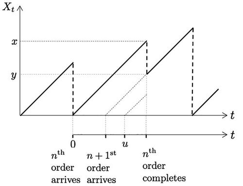
The process evolves as follows: as the production of an order continues, X_t increases linearly over time and a downward jump in X_t occurs when an order completes service. Three types of transitions can occur from state $(X_t,L_t)=(x,i):$

• A transition to state (x, j) for $j\ne i\in \mathcal{P}$ when the state of production/change-over/setup changes but the same order remains in service. Denote by ${(A_0)}_{i,j}$ as the rate of this transition.

• A transition to a state (y, j) with $y\in [x-u,x),$ for $0<u<x$ when an order completes service and there is a subsequent order in the queue enters service. When the inter-arrival time of the subsequent order is (at most) u, time units, the order has waited at least x—u time units, illustrated in Figure 1. Denote by $A_{i,j}(u)$ the transition rate, with $d{A}_{i,j}(u)$ its corresponding density function. The matrix A(u) of rates $A_{i,j}(u)$ takes into account the correlation between j (which represents the new order size) and u (the inter-arrival time between the new order and the previous one).

• A transition to state $(0,j)$ when the order completes service and the queue is empty upon service completion. This occurs with rate ${\int }_x^{\infty }d{A}_{i,j}(u).$

Figure 1. Sample path of X_t. Upon production completion of the n^th order at age x, the subsequent order in service has already spent at least x – u time units in the system.

The matrices A₀ and dA(u) are described in the next sections.

4.2. Transition rate matrix A₀

Define (2) $$A_0\mathrm{ }=\left[\begin{array}{cc}{F}_{++}^{(1)}& \mathbf{0}\\ \mathbf{0}& F_{++}^{(2)}\end{array}\right],$$(2) where $F_{++}^{(j)}$ is an order $\left|{\mathcal{P}}_j\right|$ matrix that contains the rates when the order was initiated by product j. Then (3) $$F_{++}^{(1)}=I_{m_1}\otimes \left[\begin{array}{cc}{F}_{++,\mathit{indiv}}^{(1)}& \mathbf{0}\\ \mathbf{0}& F_{++,\mathit{joint}}^{(1)}\end{array}\right],$$(3) where $I_{m_1}$ records the inventory position of product 1 the moment the order was placed, the matrices $F_{++,\mathit{joint}}^{(1)}$ and $F_{++,\mathit{indiv}}^{(1)}$ describe the joint and individual orders initiated by product 1, respectively, and ⊗ denotes the Kronecker product. Then, (4) $$F_{++,\mathit{joint}}^{(1)}=\left[\begin{array}{ccccc}{V}_{-}& & & & 0\\ v_{+}{\gamma }_{-}& V_{+}& & & \\ & u_p{\gamma }_{+}& U_p& & \\ & & \ddots & \ddots & \\ 0& & & u_p{\gamma }_p& U_p\end{array}\right],$$(4) is an order $z^{1,\mathit{joint}}$ matrix and describes the transitions in production and setup phases and where the vectors $u_p=-U_{p}e$ and $v_{+}=-V_{+}e$ denote the completion rates of the unit production and the major setup time, respectively. Define, (5) $$F_{++,\mathit{indiv}}^{(1)}=I_{S_2-c_2}\otimes \left[\begin{array}{ccccc}{V}_{+}& & & & 0\\ u_p{\gamma }_{+}& U_p& & & \\ & u_p{\gamma }_p& \ddots & & \\ & & \ddots & \ddots & \\ 0& & & u_p{\gamma }_p& U_p\end{array}\right],$$(5) an order $(S_2-c_2)z^{1,\mathit{indiv}}$ matrix. Since there is no minor setup time, we record the inventory position of product 2 with $I_{S_2-c_2},$ the moment the order was placed. Then we obtain a zero matrix, except for the $S_2-c_2$ sub-matrices on the diagonal where each of sub-matrix defines the transitions in production and setup and specifying i₂. Similarly, define (6) $$F_{++}^{(2)}=\left[\begin{array}{cc}{F}_{++,\mathit{indiv}}^{(2)}& \mathbf{0}\\ \mathbf{0}& F_{++,\mathit{joint}}^{(2)}\end{array}\right],$$(6) where (7) $$F_{++,\mathit{indiv}}^{(2)}=I_{S_1-c_1}\otimes \left[\begin{array}{ccccc}{V}_{+}& & & & 0\\ u_p{\gamma }_{+}& U_p& & & \\ & u_p{\gamma }_p& \ddots & & \\ & & \ddots & \ddots & \\ 0& & & u_p{\gamma }_p& U_p\end{array}\right],$$(7) is of order $(S_1-c_1)z^{2,\mathit{indiv}}$ and (8) $$F_{++,\mathit{joint}}^{(2)}=I_{c_1-s_1}\otimes \left[\begin{array}{ccccc}{V}_{-}& & & & 0\\ v_{+}{\gamma }_{-}& V_{+}& & & \\ & u_p{\gamma }_{+}& U_p& & \\ & & \ddots & \ddots & \\ 0& & & u_p{\gamma }_p& U_p\end{array}\right],$$(8) is of order $(c_1-s_1)z^{2,\mathit{joint}}.$ In both joint and individual orders, we keep track of the inventory position of product 1 at the moment the order was placed.

4.3. Density matrix dA(u)

The density function of the rate matrix A(u) can be expressed as (9) $$dA(u)=F_{+-}{e}^{F_{--}u}{F}_{-+},$$(9) where $F_{+-}$ describes the transitions from the states in $\mathcal{P}$ prior to service completion to the inventory positions of both products immediately after the order was placed. The matrix exponential $e^{F_{--}u}$ gives the density of the inter-arrival time of u, where $F_{--}$ describes the evolution of the inventory position until the subsequent order is placed. The matrix $F_{-+}$ describes the transitions to the initial production state of the subsequent order beginning at $t-X_t+u.$

4.3.1. Production completion of the order in service ($F_{+-}$)

Denote by α_j the vector of the steady state probabilities of the inventory position immediately after a replenishment, then ${\alpha }_j=(1,0,\dots ,0)$ with length $(S_j-s_j).$ Let (10) $$F_{+-}=\left[\begin{array}{c}{F}_{+-}^{(1)}\\ F_{+-}^{(2)}\end{array}\right],$$(10) where $F_{+-}^{(j)}$ describes the transitions when the order was initiated by j. Recalling that completion occurs after a major setup time in an individual order, or after a minor change over time of a joint order, we have (11) $$F_{+-}^{(1)}=e_{m_1}\otimes \left[\begin{array}{c}{\alpha }_1\otimes \left(I_{S_2-c_2}\otimes {\nu }_{+}^{(1)}\right)\\ {\nu }_{-}^{(1)}\left({\alpha }_1\otimes {\alpha }_2\right)\end{array}\right],$$(11) with dimensions $\left|\mathcal{P}\right|\times (S_1-s_1)(S_2-s_2)$ and where ${\nu }_{+}^{(j)}={(v_{+}^{⊺},0,\dots ,0)}^{⊺}$ is a vector of length $z^{j,\mathit{indiv}}$ and ${\nu }_{-}^{(j)}={(v_{-}^{⊺},0,\dots ,0)}^{⊺}$ a vector of length $z^{j,\mathit{joint}},$ where $v_{+}^{⊺}$ denotes the transpose of $v_{+}.$ The vector $e_{m_1}$ records the inventory level of product 1 during production as a new order is about to begin. The upper sub-matrix in Equation (11)(11) $$F_{+-}^{(1)}=e_{m_1}\otimes \left[\begin{array}{c}{\alpha }_1\otimes \left(I_{S_2-c_2}\otimes {\nu }_{+}^{(1)}\right)\\ {\nu }_{-}^{(1)}\left({\alpha }_1\otimes {\alpha }_2\right)\end{array}\right],$$(11) describes an individual order of product 1, then the inventory position of product 1 is raised to S₁ and we record the inventory position of product 2 with $I_{S_2-c_2}.$ The lower sub-matrix describes a joint order, in which case the inventory positions of both products are raised to their respective S_j. Similarly, (12) $$F_{+-}^{(2)}=\left[\begin{array}{c}{I}_{S_1-c_1}\otimes \left({\nu }_{+}^{(2)}{\alpha }_2\right)\\ \left(e_{c_1-s_1}\otimes {\nu }_{-}^{(2)}\right)\left({\alpha }_1\otimes {\alpha }_2\right)\end{array}\right],$$(12) where $I_{S_1-c_1}$ is used to keep track of the inventory position of product 1 when only product 2 is replenished, and $e_{c_1-s_1}$ records the inventory position of product 1 in a joint order.

4.3.2. Inventory position until subsequent order ($F_{--}$)

The matrix $F_{--}$ is of order $(S_1-s_1)(S_2-s_2)$ and describes the transition rates in the inventory positions of both products due to demand arrivals until the reorder point of one of the products is reached. Then (13) $$\begin{array}{c}{F}_{--}=\left[\begin{array}{cccc}-{\lambda }^{(1)}& {\lambda }^{(1)}{d}_1^{(1)}& \dots & {\lambda }^{(1)}{d}_{S_1-s_1-1}^{(1)}\\ 0& -{\lambda }^{(1)}& \dots & {\lambda }^{(1)}{d}_{S_1-s_1-2}^{(1)}\\ ⋮& & \ddots & ⋮\\ 0& \dots & 0& -{\lambda }^{(1)}\end{array}\right]\otimes I_{S_2-s_2}\\ +I_{S_1-s_1}\otimes \left[\begin{array}{cccc}-{\lambda }^{(2)}& {\lambda }^{(2)}{d}_1^{(2)}& \dots & {\lambda }^{(2)}{d}_{S_2-s_2-1}^{(2)}\\ 0& -{\lambda }^{(2)}& \dots & {\lambda }^{(2)}{d}_{S_2-s_2-2}^{(2)}\\ ⋮& & \ddots & ⋮\\ 0& \dots & 0& -{\lambda }^{(2)}\end{array}\right].\end{array}$$(13)

The time u between subsequent orders is then equivalent to the time it takes for the process to decrease from the inventory positions just after an order was placed until absorption in one of the reorder points (or below), thus its density is given by $e^{F_{--}u}.$

4.3.3. Start of production of the subsequent order ($F_{-+}$)

Let $F_{-+}=[F_{-+}^{(1)}{F}_{-+}^{(2)}]$ where $F_{-+}^{(j)}$ records the transitions when the order was initiated by product j and which has dimension $(S_1-s_1)(S_2-s_2)\times \left|{\mathcal{P}}_j\right|.$ Then (14) $$F_{-+}^{(1)}=\sum _{k=0}^{m_1-1}\left({\eta }_k^{(1)}\otimes I_{S_2-s_2}\right){\Gamma }_k^{(1)},$$(14) where (15) $${\eta }_k^{(j)}={\left[\begin{array}{ccccccc}{\lambda }^{(j)}{d}_{S_j-s_j+k}^{(j)}& {\lambda }^{(j)}{d}_{S_j-s_j+k-1}^{(j)}& \dots & {\lambda }^{(j)}{d}_{k+1}^{(j)}& 0& \dots & 0\end{array}\right]}^{⊺},$$(15) is a column vector ${\eta }_k^{(j)}$ of length $S_j-s_j$ and contains the rates of demand arrivals for product 1 which result in an order of size $S_1-s_1+k.$ The matrix ${\Gamma }_k^{(1)}$ determines the state in which production starts if the order size of product 1 equals $S_1-s_1+k$ and if the inventory position of product 2 is $S_2-i_2+1$ at the moment when product 1 initiates an order, for $i_2=1,\dots ,S_2-s_2.$ If only product 1 is replenished, ${\Gamma }_k^{(1)}$ also records the inventory position of product 2, i₂. Thus ${\Gamma }_k^{(1)}$ is an $(S_2-s_2)\times \left|{\mathcal{P}}_1\right|$ matrix with all its entries equal to zero, except for n_p entries given by γ_p. For $i_2=1,\dots ,S_2-c_2$ the inventory position of product 2 remains above c₂ and the n_p nonzero entries of row i₂ of ${\Gamma }_k^{(1)}$ are on the columns corresponding to the states $(k,S_2-i_2+1,n_s^{+}+z)\in {\mathcal{P}}_{1,\mathit{indiv}}$ with $z=(S_1-s_1+k-1)n_p+1$ to $(S_1-s_1+k)n_p.$ For $i_2=S_2-c_2+1,\dots ,S_2-s_2$ we have a joint order and the n_p nonzero entries on row i₂ of ${\Gamma }_k^{(1)}$ are on the columns corresponding to the states $(k,n_s^{-}+n_s^{+}+z)$ of ${\mathcal{P}}_{1,\mathit{joint}}$ with $z=(S_1-s_1+k+i_2-2)n_p+1$ to $(S_1-s_1+k+i_2-1)n_p$ as the joint order has size $S_1-s_1+k+i_2-1.$

Similarly, $F_{-+}^{(2)}$ defines the transition rates when product 2 reaches its reorder point, (16) $$F_{-+}^{(2)}=\sum _{k=0}^{m_2-1}\left(I_{S_1-s_1}\otimes {\eta }_k^{(2)}\right){\Gamma }_k^{(2)},$$(16) with ${\Gamma }_k^{(2)}$ an $(S_1-s_1)\times \left|{\mathcal{P}}_2\right|$ matrix with all its entries equal to zero, except that each row contains n_p entries equal to γ_p. More specifically, the non-zero entries on row $i_1\in \{1,\dots ,S_1-c_1\}$ appear on the columns corresponding to the states $(i_1,n_{+}+z)\in {\mathcal{P}}_{2,\mathit{indiv}}$ with $z=(S_2-s_2+k-1)n_p+1$ to $z=(S_2-s_2+k)n_p.$ For $i_1\in \{S_1-c_1+1,\dots ,S_1-s_1\}$ the columns corresponding to the states $(i_1,n_{-}+n_{+}+z)$ of ${\mathcal{P}}_{2,\mathit{joint}}$ with $z=(S_2-s_2+k+i_1-2)n_p+1$ to $(S_2-s_2+k+i_1-1)n_p$ holds the entries of γ_p.

4.4. Utilization of the production system

Define ρ_p as the production utilization rate, that is, excluding the setup times, then (17) $${\rho }_p=\sum _{j=1}^2(-{\lambda }^{(j)}{\gamma }_p{U}_p^{-1}e\sum _{i=1}^{m_j}i{d}_i^{(j)}),$$(17) where ${\gamma }_p{(-U_p)}^{-1}e$ is the mean unit production time and ${\sum }_{i=1}^{m_j}i{d}_i^{(j)}$ is the mean demand size for product j. The overall utilization ρ is then determined by the number of orders placed, (18) $$\rho ={\rho }_p-\left({\gamma }_{+}{V}_{+}^{-1}e+{\gamma }_{-}{V}_{-}^{-1}e\right)({\eta }_1^c+{\eta }_2^c)-\left({\gamma }_{+}{V}_{+}^{-1}e\right)({\eta }_1+{\eta }_2),$$(18) where $-{\gamma }_{+}{V}_{+}^{-1}e$ and $-{\gamma }_{-}{V}_{-}^{-1}e$ are the mean major setup and minor change-over times, respectively.

5. Steady-state analysis

We consider the form of steady state of the Markov process in Section 5.1 and construct the associated fluid queue in Section 5.2. In Section 5.3 we obtain an expression for the inventory position and the number of demand arrivals since an order was placed and combine the results to determine the inventory level distribution.

5.1. Preliminaries

For x > 0, $j\in \mathcal{P},$ denote the steady-state density of (X_t, L_t) as (19) $${\delta }_j(x)=\underset{t\to \infty }{\lim }\frac{d}{dx}P\left[X_t<x,L_t=j\right],$$(19) and the corresponding vector $\delta (x)=\{{\delta }_j(x),j\in \mathcal{P}\}.$ If $\rho <1$ the process (X_t, L_t) has matrix exponential form^[31,32] and there exists a matrix T of order $\left|\mathcal{P}\right|$ such that (20) $$\delta (x)=\delta (0)e^{Tx},$$(20) where the matrix T is the smallest non-negative solution to (21) $$T=A_0+{\int }_0^{\infty }{e}^{Tx}dA(x),$$(21) and $\delta (0)=\theta (-T),$ where θ is the stationary vector of (22) $$A=A_0+{\int }_0^{\infty }dA(u).$$(22)

See Van Houdt^[37] for details.

Using the matrices A₀ and dA(x), the matrix T can be computed iteratively, $T_{n+1}=A_0+{\int }_0^{\infty }{e}^{T_{n}x}dA(x),$ with $T_0=0$^[31]. As this method results in linear convergence and is therefore impractical under high loads, in the next section we present a more efficient approach.

5.2. Reduction to a fluid queue

To employ a method for computing T that converges quadratically we construct a fluid queue^[13]. In order to obtain a fluid queue, the fluid process must be skip-free in both directions so we replace the immediate downward jumps in X_t by intervals of the appropriate length during which the level decreases linearly. Then there are $\left|\mathcal{P}\right|$ phases in which the fluid increases and $\left|\mathcal{I}\right|$ artificial phases in which the fluid decreases and the rate matrix of the underlying continuous-time Markov chain is (23) $$F=\left[\begin{array}{cc}{F}_{++}& F_{+-}\\ F_{-+}& F_{--}\end{array}\right].$$(23)

The matrix $F_{++}=A_0$ contains the rates at which the phase changes while the fluid increases (the same order remains in service), $F_{+-}$ contains the transitions from an increase to a decrease in fluid (a service completion occurs), $F_{-+}$ contains the transitions from a decrease to an increase in fluid (a new order enters service) and $F_{--}$ contains the transition rates while the fluid decreases (demands arrive depleting the inventory, but no product has reached its order point).

When the fluid queue hits level zero the phase continues to evolve according to $F_{--}$ until an event part of $F_{-+}$ occurs and the fluid level becomes positive again. Censoring the queue only on the periods where the level increases we obtain the Markov process of Section 4, in which the age always increases, unless there is a downward jump. Due to Equation (9)(9) $$dA(u)=F_{+-}{e}^{F_{--}u}{F}_{-+},$$(9) , a downward jump to level zero occurs with rate ${\int }_x^{\infty }d{A}_{i,j}(u)={(F_{+-}{e}^{F_{--}x}{(-F_{--})}^{(-1)}{F}_{+-})}_{i,j}$ where the part ${(-F_{--})}^{(-1)}{F}_{+-}$ captures the evolution of the phase of the fluid queue at zero.

If we take the expression for the steady state of a fluid queue^[23] and observe the queue only when the level is increasing, the steady state has the form given in Equation (20)(20) $$\delta (x)=\delta (0)e^{Tx},$$(20) with (24) $$T=F_{++}+\Psi F_{-+},$$(24) and $\delta (0)=\theta (-T),$ where θ is the stationary vector of $A=A_0+F_{+-}{(-F_{--})}^{-1}{F}_{-+}$ and matrix $\Psi ,$ the first return probabilities to the initial level, is the minimal non-negative solution to an algebraic Riccati equation (25) $$\Psi F_{-+}\Psi +F_{++}\Psi +\Psi F_{--}+F_{+-}=0.$$(25)

To reduce the computation time of θ, we employ the power method^[39]. Further, as $F_{++}$ has block diagonal form, we can apply the algorithm of Meini^[25], which exploits this structure to reduce the memory and time complexity.

Observing the phase process only during the intervals of time in which the fluid level is decreasing, that is, when the production facility is idle, the rate matrix is (26) $$D=F_{--}+F_{-+}\Psi .$$(26) from which we obtain the steady state probabilities of the idle production facility, $\widehat{\theta },$ such that $\widehat{\theta }D=0,\widehat{\theta }e=1.$

5.3. Inventory level distribution of product 1

For $i\ge 0,$ denote by ${\varphi }_i$ the probability the inventory level is $S_1-i.$ To derive this distribution, we separately consider the situations in which the server is busy and where it is idle.

Firstly when the server is busy, define $q_{k,n}$ as the probability that the inventory position of product 1 was $S_1-k$ at the moment when the order in production was placed and n demand arrivals of product 1 have depleted inventory since. The corresponding vector $q_n=\{q_{k,n},k=0,1,\dots ,o^{(1)}\}$ is partitioned such that (27) $$q_n=\left[q_{(0:S_1-c_1-1),n}{q}_{(S_1-c_1:S_1-s_1-1),n}{q}_{(S_1-s_1:o^{(1)}),n}\right],$$(27) where the entries refer to individual orders placed by product 2, joint orders initiated by product 2, and orders initiated by product 1 (joint or individual), respectively. During the time x this order has spent in the system, the probability that the inventory is further depleted by the arrival of n demands for product 1 is $(1/n!){({\lambda }^{(1)}x)}^n{e}^{-({\lambda }^{(1)}x)}.$ Let (28) $$p_n(x)={\int }_0^{\infty }\delta (x)\frac{{\left({\lambda }^{(1)}x\right)}^n}{n!}{e}^{-{\lambda }^{(1)}x}dx=\delta (0){\left({\lambda }^{(1)}\right)}^n{\left({\lambda }^{(1)}{I}_{\left|\mathcal{P}\right|}-T\right)}^{-(n+1)},$$(28) then $q_n=p_n(x)\left[(I_{m_1}\otimes e_{\left|{\mathcal{P}}_1\right|/m_1}),(I_{c_1-s_1}\otimes e_{z^{2,\mathit{joint}}}),(I_{S_1-c_1}\otimes e_{z^{2,\mathit{indiv}}})\right].$

We can then write (29) $${\varphi }_i=\left(1-\rho \right)g_i+\rho f_i,$$(29) where $1-\rho$ is the probability of a idle server in which the inventory level of product 1 is at least $s_1+1$ and the idle probabilities g_i are given by (30) $$g_i={\left(\widehat{\theta }(I_{S_1-s_1}\otimes e_{S_2-s_2})\right)}_{i+1}1[0\le i\le S_1-1],$$(30) where $\widehat{\theta }$ is derived from the fluid queue construction in Equation (26)(26) $$D=F_{--}+F_{-+}\Psi .$$(26) and where $1[A]=1$ if A is true and $1[A]=0$ otherwise.

When the server is busy, with probability ρ, ${\varphi }_i$ is obtained by $q_{k,n}$ and the n-fold convolution of the demand size distribution, (31) $$f_i=\sum _{\begin{array}{c}k\le i,\\ n\le i-k\end{array}}{q}_{k,n}\sum _{\begin{array}{c}{k}_1,\dots ,k_n>0,\\ k_1+\dots +k_n=i-k\end{array}}\prod _{s=1}^n{d}_{k_s}^{(1)}.$$(31)

Then the expected number of units in inventory and expected number of units backlogged are (32) $${\Phi }_1^{+}=\sum _{i=0}^{S_1}{\varphi }_i(S_1-i),\hspace{1em}{\Phi }_1^{-}=\sum _{i=S_1+1}^{\infty }{\varphi }_i(i-S_1).$$(32)

Denote by L the lead time and define $\zeta (x)$ as its steady state density, (33) $$\zeta (x)=\frac{\delta (x)\widehat{\eta }}{{\int }_0^{\infty }\delta (y)\widehat{\eta }dy}=\frac{\theta (-T)e^{Tx}\widehat{\eta }}{\theta \widehat{\eta }},$$(33) where $\widehat{\eta }=F_{+-}e,$ and with corresponding distribution function (34) $$Z(x)=1-\frac{\theta e^{Tx}\widehat{\eta }}{\theta \widehat{\eta }},$$(34) then the expected lead time of a random order is $E[L]=-\theta T^{-1}\widehat{\eta }{(\theta \widehat{\eta })}^{-1}.$ Conditioning on the order if product 1 is included, the product dependent expected lead time is (35) $$E\left[L^{(j)}\right]=-\theta T^{-1}{\widehat{\eta }}^{(j)}{(\theta {\widehat{\eta }}^{(j)})}^{-1},$$(35) where (36) $${\widehat{\eta }}^{(1)}=\left[\begin{array}{c}{F}_{+-}^{(1)}\\ I_{S_1-c_1}\otimes \left({\nu }_{+}^{(2)}{\alpha }_2\right)\\ \left(e_{c_1-s_1}\otimes {\nu }_{-}^{(2)}\right)\left({\alpha }_1\otimes {\alpha }_2\right)\end{array}\right]°\left[\begin{array}{c}\mathbf{1}\\ \mathbf{0}\\ \mathbf{1}\end{array}\right],$$(36) using the expression for $F_{+-}^{(2)}$ in Equation (12)(12) $$F_{+-}^{(2)}=\left[\begin{array}{c}{I}_{S_1-c_1}\otimes \left({\nu }_{+}^{(2)}{\alpha }_2\right)\\ \left(e_{c_1-s_1}\otimes {\nu }_{-}^{(2)}\right)\left({\alpha }_1\otimes {\alpha }_2\right)\end{array}\right],$$(12) , and where $°$ denotes the Hadamard product.

6. Expected total cost

For the computation of the expected total cost, we need to characterize the time between orders. In Section 6.1 we consider the time, η_j, between individual orders, and similarly in Section 6.2 for the time, ${\eta }_j^c,$ between joint orders. In Section 6.3 we present the iterative procedure employed to derive the policy parameters for both products and give numerical illustrations.

6.1. Expected number of individual orders per unit time

The time between two subsequent individual orders has distribution $PH({\widehat{\pi }}_j,{\widehat{F}}_{--}^{(j)})$ of order $(S_1-s_1)(S_2-s_2)$ and the time to place the subsequent order is equivalent to the time to reach absorption. The expected time between subsequent individual orders of product j is given by ${\eta }_j^{-1}={\widehat{\pi }}_j{(-{\widehat{F}}_{--}^{(j)})}^{-1}e.$ Define (37) $$D^{(j)}=\left[\begin{array}{c}\sum _{k=0}^{m_j-1}{\lambda }^{(j)}{d}_{S_j-s_j+k}^{(j)}\\ ⋮\\ \sum _{k=0}^{m_j-1}{\lambda }^{(j)}{d}_{1+k}^{(j)}\end{array}\right].$$(37)

The matrix $F_{--}$ records the transitions in inventory position until the subsequent replenishment, thus only a decrease in inventory positions is possible. However in ${\widehat{F}}_{--}^{(j)},$ an increase in inventory positions is possible when product $i\ne j$ places an order. Then for j = 1, (38) $${\widehat{F}}_{--}^{(1)}\mathrm{ }=F_{--}+D^{(1)}{\alpha }_1\otimes \left[\begin{array}{c}0\\ e_{c_2-s_2}{\alpha }_2\end{array}\right]+\left[\begin{array}{c}\begin{array}{cc}{I}_{S_1-c_1}& 0\end{array}\\ e_{c_1-s_1}{\alpha }_1\end{array}\right]\otimes D^{(2)}{\alpha }_2,$$(38) where the second term refers to an increase in inventory positions due to a joint order initiated by product 1, and the third term refers to a (joint or individual) order placed for product 2. The vector ${\widehat{\pi }}_1$ contains the probabilities of starting in a given state following an individual order of product 1 and is the stationary distribution of $${\left(-{\widehat{F}}_{--}^{(1)}\right)}^{-1}\left(D^{(1)}{\alpha }_1\otimes \left[\begin{array}{cccc}{I}_{S_2-c_2}& 0& \dots & 0\\ 0& 0& \dots & 0\\ ⋮& ⋮& & ⋮\\ 0& 0& \dots & 0\end{array}\right]\right),$$ as an individual order for product 1 can only occur if the inventory position of product 2 is at least $c_2+1.$ Similarly, (39) $${\widehat{F}}_{--}^{(2)}\mathrm{ }=F_{--}+D^{(1)}{\alpha }_1\otimes \left[\begin{array}{c}\begin{array}{cc}{I}_{S_2-c_2}& 0\end{array}\\ e_{c_2-s_2}{\alpha }_2\end{array}\right]+\left[\begin{array}{c}0\\ e_{c_1-s_1}{\alpha }_1\end{array}\right]\otimes D^{(2)}{\alpha }_2,$$(39) and ${\widehat{\pi }}_2$ is the stationary distribution of $$\begin{array}{c}{\left(-{\widehat{F}}_{--}^{(2)}\right)}^{-1}\left(\left[\begin{array}{cccc}{I}_{S_1-c_1}& 0& \dots & 0\\ 0& 0& \dots & 0\\ ⋮& ⋮& & ⋮\\ 0& 0& \dots & 0\end{array}\right]\otimes D^{(2)}{\alpha }_2\right).\hfill \end{array}$$

6.2. Expected number of joint orders per unit time

The time between two subsequent joint orders initiated by product 1 has distribution $PH({\alpha }_1\otimes {\alpha }_2,{\widehat{F}}_{--}^{(12)}),$ then ${({\eta }_1^c)}^{-1}=({\alpha }_1\otimes {\alpha }_2){(-{\widehat{F}}_{--}^{(12)})}^{-1}e.$ As the inventory position of both products after placing a joint order is $(S_1,S_2),$ the initial state vector is ${\alpha }_1\otimes {\alpha }_2$ and (40) $${\widehat{F}}_{--}^{(12)}\mathrm{ }=F_{--}+D^{(1)}{\alpha }_1\otimes \left[\begin{array}{cc}{I}_{S_2-c_2}& 0\\ 0& 0\end{array}\right]+\left[\begin{array}{c}\begin{array}{cc}{I}_{S_1-c_1}& 0\end{array}\\ e_{c_1-s_1}{\alpha }_1\end{array}\right]\otimes D^{(2)}{\alpha }_2,$$(40) where the second term accounts for the individual orders placed of product 1, and the third term refers for the orders placed by product 2. The time between two subsequent joint orders initiated by product 2 is $PH({\alpha }_1\otimes {\alpha }_2,{\widehat{F}}_{--}^{(21)})$ with ${({\eta }_2^c)}^{-1}=({\alpha }_1\otimes {\alpha }_2){(-{\widehat{F}}_{--}^{(21)})}^{-1}e,$ where (41) $${\widehat{F}}_{--}^{(21)}\mathrm{ }=F_{--}+D^{(1)}{\alpha }_1\otimes \left[\begin{array}{c}\begin{array}{cc}{I}_{S_2-c_2}& 0\end{array}\\ e_{c_2-s_2}{\alpha }_2\end{array}\right]+\left[\begin{array}{cc}{I}_{S_1-c_1}& 0\\ 0& 0\end{array}\right]\otimes D^{(2)}{\alpha }_2.$$(41)

6.3. Iterative solution and numerical examples

To obtain the inventory parameters that minimize $E[C]$ in Equation (1)(1) $$\begin{array}{c}E\left[C\right]=\sum _{j=1}^2\left((\tilde{k}+k_j)({\eta }_j+{\eta }_j^c)+k_j{\eta }_{3-j}^c+h_j{\Phi }_j^{+}+p_j{\Phi }_j^{-}\right),\end{array}$$(1) , we use an iterative procedure to obtain successive approximations for both products using neighbor search and steepest descent algorithms. Given a set of initial inventory parameters for product 1, we determine the optimal inventory parameters for product 2. Then given this inventory policy for product 2, we determine the inventory parameters for product 1 that minimize $E[C]$ and repeat until convergence is reached. We note that to compute the cost for both products simultaneously would involve matrices with significantly larger dimensions and hence be less tractable.

We present results for six experiments for different values of the ordering costs and minor change-over times, as these drive the order quantities, $(S_j-s_j)$ and $(S_j-c_j).$ The parameter values are chosen to highlight the impact of changing the key replenishment drivers and costs, being the ordering costs and setup times. The holding and backlogging costs represent a service level of 90%. Parameter values common to all experiments are listed in Table 2 and the different values are listed in Table 3. The unit production time, major setup and minor change-over times are each exponentially distributed and the demand size distribution is zero-truncated binomial.

Table 2. Parameter values common to all numerical experiments.

Parameter	Product 1	Product 2
${\lambda }^{(j)}$ (per hour)	1	1
Maximum demand size mj	8	6
Mean demand size	4	3
Holding cost hj (per hour)	1	2
Backlogging cost pj (per hour)	9	18
Mean unit production time (hours)	1/12	1/12
Mean major setup (hours)	1/2	1/2

Table 3. Ordering costs and setup times for each experiment.

Experiment	$\tilde{k}$	k1	k2	Mean minor change-over (hours)
1	8	2	0	1/4
2	8	2	0	1/100
3	0	10	8	1/4
4	0	10	8	1/100
5	0	0	0	1/4
6	0	0	0	1/100

We demonstrate the iterative procedure for deriving parameters for the case of an independent replenishment $(s_j,S_j)$ policy and discuss the interplay between the quantities of interest. We then illustrate the cost reduction by using a joint replenishment policy compared to independent policy.

Obtaining cost minimizing parameters for individual replenishment. For Experiment 1, we outline the solution for $(s_j^{*},S_j^{*}).$ The iterations are listed in Table 4 with an initial guess of $S_1-s_1=5,$ from which we obtain $(s_1^{*},S_1^{*})=(16,38)$ and $(s_2^{*},S_2^{*})=(11,27).$

Table 4. Parameters obtained for the iterative procedure in Experiment 1 for $(s_j^{*},S_j^{*}).$

Iteration	Input	Output	Status
1	$S_1-s_1=5$	$(s_2,S_2)=(26,78)$	$\rho =0.91,E[C]=252.82$
2	$S_2-s_2=52$	$(s_1,S_1)=(20,39)$	$\rho =0.71,E[C]=102.01$
3	$S_1-s_1=19$	$(s_2,S_2)=(11,27)$	$\rho =0.77,E[C]=61.55$
4	$S_2-s_2=16$	$(s_1,S_1)=(16,38)$	$\rho =0.75,E[C]=60.74$
5	$S_1-s_1=22$	$(s_2,S_2)=(11,27)$	$\rho =0.75,E[C]=60.74$

To understand how the quantities of interest change throughout the iteration, Figures 2–4 illustrate how ρ, $E[C]$ and s_j evolve.

Figure 2. Order quantity $(S_j-s_j)$ vs. utilization rate ρ.

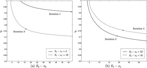
Figure 3. Order quantity $(S_j-s_j)$ vs. reorder points $(s_j^{*}).$

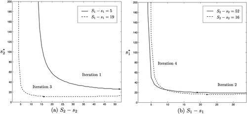
Figure 4. Order quantity $(S_j-s_j)$ vs. expected total cost $E[C].$

Iteration 1. For the initial order quantity $S_1-s_1=5,$ the small size leads to multiple setups, congested production, long lead times and high costs. The solid line Figure 2(a) illustrates how ρ decreases as the order quantity of product 2 increases. The cost-minimizing reorder point s₂ as a function of the order quantity is illustrated in Figures 3(a) and 4(a) illustrates the impact on $E[C].$ Due to the small order of product 1, a large order of product 2 is optimal, as this tempers the utilization rate and lead times.

Iteration 2. Given $S_2-s_2=52,$ the solid lines of Figures 2–4(b) illustrate the impact of the order quantity of product 1 on the utilization rate ρ, optimal reorder point s₁ and expected total costs $E[C],$ respectively. Increasing the order quantity of product 1 from 5 to 19, leads to more favorable lead times (due to a reduction in setups) and lower total system costs.

Iteration 3. Given $S_1-s_1=19,$ the dashed lines of Figures 2–4(a) illustrate how $S_2-s_2$ impacts ρ, $s_2^{*}$ and $E[C],$ respectively. Compared to the scenario in Iteration 1, the order quantity of 1 is larger, thus the order quantity of 2 can be reduced to 16 units while $E[C]$ is also reduced.

Iterations 4 and 5. Given $S_2-s_2=16,$ the dashed lines in Figures 2–4(b) illustrate quantities for iteration 4. We obtain $(s_1,S_1)=(16,38)$ with $E[C]=60.74$ and $\rho =0.75.$ Proceeding to the next iteration with $S_1-s_1=22,$ we find $(s_2,S_2)=(11,27)$ thus the procedure ends and the optimal inventory parameters are $(s_1^{*},S_1^{*})=(16,38)$ and $(s_2^{*},S_2^{*})=(11,27).$

The results for the all experiments are listed in Table 5. As expected, the minor change-over time has no impact as no joint orders are placed. Different values of $\tilde{k}$ and k_j have no impact as long as $\tilde{k}+k_j$ remains the same for product j, which explains why the result of experiments $1-4$ are the same for the (s_j, S_j) policy. In experiments 5 and 6 $\tilde{k}+k_j=0$ and the optimal order quantities are only slightly smaller compared to experiments $1-4$ due to the impact of the order quantities on setup times and lead times.

Table 5. Optimal replenishment parameters for each experiment.

Optimal replenishment parameters of product 1
Exp.	$(s_1^{*},S_1^{*})$	$E[C]$	η1	$E[L]$	$(s_1^{*},c_1^{*},S_1^{*})$	$E[C]$	η1	${\eta }_1^c$	$E[L]$
1	(16,38)	24.77	0.17	3.37	(18,24,38)	24.16	0.07	0.08	3.72
2	(16,38)	24.77	0.17	3.37	(16,28,33)	22.40	0.02	0.13	3.16
3	(16,38)	24.77	0.17	3.37	(18,22,39)	24.64	0.09	0.06	3.72
4	(16,38)	24.77	0.17	3.37	(15,25,33)	23.22	0.03	0.11	3.23
5	(17,38)	23.08	0.18	3.33	(18,23,37)	22.53	0.08	0.08	3.67
6	(17,38)	23.08	0.18	3.33	(15,29,32)	20.76	0.01	0.13	3.10
Optimal replenishment parameters of product 2
Exp.	$(s_2^{*},S_2^{*})$	$E[C]$	η2	$E[L]$	$(s_2^{*},c_2^{*},S_2^{*})$	$E[C]$	η2	${\eta }_2^c$	$E[L]$
1	(11,27)	35.97	0.17	3.01	(12,19,27)	34.68	0.08	0.05	3.49
2	(11,27)	35.97	0.17	3.01	(11,22,24)	31.92	0.03	0.11	3.11
3	(11,27)	35.97	0.17	3.01	(12,18,27)	35.13	0.11	0.03	3.36
4	(11,27)	35.97	0.17	3.01	(11,20,24)	32.88	0.05	0.10	3.12
5	(12,27)	34.50	0.18	2.98	(12,19,27)	33.64	0.09	0.04	3.44
6	(12,27)	34.50	0.18	2.98	(11,22,23)	30.64	0.02	0.14	3.08

Comparison of independent and joint replenishments. Following a similar iterative procedure, we present the solutions for $(s_j,c_j,S_j)$ in Table 5. In Table 6, we give the cost reductions of (s, c, S) compared to the (s, S) policy, listed alongside the ratios of the fixed ordering costs $\tilde{k}/k_j$ and the mean setup time vs. the mean change-over time. As expected, $E[C]$ is lower in the joint replenishment scenarios.

Table 6. Ratio of ordering costs and setup times.

Exp.	$\frac{\tilde{k}}{k_j}$	$\frac{E\left[\text{Setup}\right]}{E\left[\text{Change}-\text{over}\right]}$	% Cost reduction
1	8	2	3.13%
2	8	50	10.57%
3	0	2	1.60%
4	0	50	7.64%
5	$\infty$	2	2.45%
6	$\infty$	50	10.73%

In Experiment 6, due to the small change-over time, we find the highest gains with a cost reduction of 10.73%, in which the benefit is mostly seen from the reduction in setup time by placing joint orders. We see the benefit of joint replenishment is not only influenced by the ratio of $\tilde{k}/k_j,$ but also by the ratio of the joint major setup time and the changeover time. Comparing the individual and joint policies we find that the mean number of orders placed reduces in our set of experiments by more than 14%.

We demonstrate that this cost discrepancy increases in the ratio of $\tilde{k}$ and k_j and in the ratio of the major setup time and the minor change-over time. The impact of a can order policy on lead times is unclear. Although the number of setups reduces, lead times may not necessarily go down due to a batching time, i.e., waiting time after production until the joint order is completed.

7. Concluding remarks

The analysis of sufficiently detailed production-inventory models is challenging when accounting for the number of variable quantities in the supply-chain process. We consider a continuous review finite capacity production-inventory system with two products in inventory. As the order process of each individual product impacts the utilization rate of the production system and thus the lead times for all products, the inventory levels are mutually dependent.

The contribution of this work is to construct an exact evaluation for the can-order joint replenishment policy while taking endogenous lead times into account and hence, using numerical examples, to study the complex interplay between product inventory levels, adding to the relatively limited studies of multi-item inventory analysis. The analysis in the current paper allows for systems with batch demand arrivals, variable order quantities, and non-exponential production times. Modeling the production facility as a multi-type queue, with correlated arrivals and type dependent service, the matrix exponential form of the age process of the busy queue is used to compute the inventory level distribution. For a given set of input values, our analysis generates parameters to specify a minimal cost can-order policy, a well-known heuristic for the joint replenishment problem.

We use numerical methods to obtain inventory parameters that minimize total ordering and holding costs and provide examples of the interaction between the inventory properties for the two product case, in terms of lead times, order quantities, and cost reductions from a can-order joint replenishment policy as compared with an independent order-up-to policy. We demonstrate scenarios where there is decreased cost of a can-order (s, c, S) joint replenishment policy as compared with an independent order-up-to (s, S) policy. Our analysis also can apply to a setting with multiple retailers of a single product that is produced on the same production line^[41] and joint replenishment in transport applications^[30]. A limitation is the computation time, which grows rapidly with the number of products, the maximum demand size or the order quantity. The analysis is applicable to more products but further work includes establishing optimality of the solution obtained numerically, and development of heuristics to manage combinatorial state space explosion. The analysis can be extended to a system with MAP arrival processes, however, this will increase the dimension of the matrices involved (by a factor equal to the product of the number of states of both MAPs).

Additional information

Funding

This research was supported by the Research Foundation-Flanders (FWO-Vlaanderen), grant no. G069016N. This work was also supported by the Additional Funding Programme for Mathematical Sciences, delivered by EPSRC (grant no. EP/V521917/1) and the Heilbronn Institute for Mathematical Research.

References

- Arrow, K.; Harris, T.; Marschak, J. Optimal inventory policy. Economet: J. Economet. Soc. 1951, 19, 250–272. pages DOI: https://doi.org/10.2307/1906813.
- Artalejo, J.; Gómez-Corral, A.; He, Q. Markovian arrivals in stochastic modelling: A survey and some new results. Stat. Oper. Res.Trans. 2010, 34, 101–144.
- Asmussen, S.; Kella, O. A multi-dimensional martingale for Markov additive processes and its applications. Adv. Appl. Probab. 2000, 32, 376–393. DOI: https://doi.org/10.1239/aap/1013540169.
- Atkins, D.; Iyogun, P. Periodic versus can-order policies for coordinated multi-item inventory systems. Manage. Sci. 1988, 34, 791–796. DOI: https://doi.org/10.1287/mnsc.34.6.791.
- Balintfy, J. On a basic class of multi-item inventory problems. Manage. Sci. 1964, 10, 287–297. DOI: https://doi.org/10.1287/mnsc.10.2.287.
- Barron, Y. Critical level policy for a production-inventory model with lost sales. Int. J. Prod. Res. 2019, 57, 1685–1705. DOI: https://doi.org/10.1080/00207543.2018.1504243.
- Barron, Y. The continuous (S, s, Se) inventory model with dual sourcing and emergency orders. Eur. J. Oper. Res. 2021, 1–21. DOI: https://doi.org/10.1016/j.ejor.2021.09.021.
- Bastos, L.; Mendes, M.; Nunes, D.; Melo, A.; Carneiro, M. A systematic literature review on the joint replenishment problem solutions: 2006–2015. Production 2017, 27, 1–11. DOI: https://doi.org/10.1590/0103-6513.222916.
- Boute, R.; Lambrecht, M.; Van Houdt, B. Performance evaluation of a production/inventory system with periodic review and endogenous lead times. Naval Res. Logist. 2007, 54, 462–473. DOI: https://doi.org/10.1002/nav.20222.
- Chakravarthy, S.; Rao, B. Queuing-inventory models with MAP demands and random replenishment opportunities. Mathematics 2021, 9, 1092. DOI: https://doi.org/10.3390/math9101092.
- Cohen-Hillel, T.; Yedidsion, L. The periodic joint replenishment problem is strongly NP-hard. Math. Oper. Res. 2018, 43, 1269–1289. DOI: https://doi.org/10.1287/moor.2017.0904.
- Dizbin, N.; Tan, B. Optimal control of production-inventory systems with correlated demand inter-arrival and processing times. Int. J. Prod. Econ. 2020, 228, 107692. DOI: https://doi.org/10.1016/j.ijpe.2020.107692.
- Dzial, T.; Breuer, L.; da Silva Soares, A.; Latouche, G.; Remiche, M. Fluid queues to solve jump processes. Perform. Eval. 2005, 62, 132–146. DOI: https://doi.org/10.1016/j.peva.2005.07.013.
- Faaland, B.; McKay, M.; Schmitt, T. A fixed rate production problem with poisson demand and lost sales penalties. Prod. Oper. Manage. 2019, 28, 516–534. DOI: https://doi.org/10.1111/poms.12931.
- He, Q. Age process, workload process, sojourn times, and waiting times in a discrete time SM[K]/PH[K]/1/FCFS Queue. Queueing Syst. 2005, 49, 363–403. ( DOI: https://doi.org/10.1007/s11134-005-6972-y.
- He, Q.; Alfa, A. The MMAP[K]/PH[K]/1 queues with a last-come-first-served preemptive service discipline. Queueing Syst. 1998, 29, 269–291. DOI: https://doi.org/10.1023/A:1019140332008.
- He, Q.; Neuts, M. Markov chains with marked transitions. Stoch. Process. Appl. 1998, 74, 37–52. DOI: https://doi.org/10.1016/S0304-4149(97)00109-9.
- Horvath, G. Efficient analysis of the MMAP[K]/PH[K]/1 priority queue. Eur. J. Oper. Res. 2015, 246, 128–139. DOI: https://doi.org/10.1016/j.ejor.2015.03.004.
- Horvath, G.; Van Houdt, B. A multi-layer fluid queue with boundary phase transitions and its application to the analysis of multi-type queues with general customer impatience. In Proceedings of the 2012 Ninth International Conference on Quantitative Evaluation of Systems. IEEE Computer Society, 2012; 23–32.
- Kayi, E.; Bilgi, T.; Karabulut, D. A note on the can-order policy for the two-item stochastic joint-replenishment problem. IIE Trans. 2008, 40, 84–92.
- Krishnamurthy, A.; Seethapathy, D. Production inventory models for a multi-product batch production system. In Rapid Modelling and Quick Response; Springer: London, 2010; 47–59.
- Kulkarni, V.; Yan, K. Production-inventory systems in stochastic environment and stochastic lead times. Queueing Syst. 2012, 70, 207–231. DOI: https://doi.org/10.1007/s11134-011-9272-8.
- Latouche, G. Structured Markov Chains in Applied Probability and Numerical Analysis. In MAM 2006: Markov Anniversary Meeting; C&M Online Media, Inc.: North Carolina, USA, 2006; 69–78.
- Latouche, G.; Ramaswami, V. Introduction to Matrix Analytic Methods in Stochastic Modeling. ASA-SIAM Series on Statistics and Applied Probability. Society for Industrial and Applied Mathematics: USA, 1999.
- Meini, B. On the numerical solution of a structured nonsymmetric algebraic Riccati equation. Perform. Eval. 2013, 70, 682–690. DOI: https://doi.org/10.1016/j.peva.2013.04.001.
- Nasr, W. Inventory systems with stochastic and batch demand: computational approaches. Ann. Oper. Res. 2022, 309, 163–125. DOI: https://doi.org/10.1007/s10479-021-04186-x.
- Neuts, M. F. Matrix-Geometric Solutions for Stochastic Models. John Hopkins University Press: Baltimore, 1994.
- Noblesse, A.; Boute, R.; Lambrecht, M.; Van Houdt, B. Lot sizing and lead time decisions in production/inventory systems. Int. J. Prod. Econ. 2014, 155, 351–360. DOI: https://doi.org/10.1016/j.ijpe.2014.04.027.
- Otten, S.; Krenzler, R.; Daduna, H. Separable models for interconnected production-inventory systems. Stoch. Models 2020, 36, 48–93. DOI: https://doi.org/10.1080/15326349.2019.1692667.
- Padilla Tinoco, S.; Creemers, S.; Boute, R. Collaborative shipping under different cost-sharing agreements. Eur. J. Oper. Res. 2017, 263, 827–837. DOI: https://doi.org/10.1016/j.ejor.2017.05.013.
- Sengupta, B. Markov processes whose steady state distribution is matrix-exponential with an application to the GI/PH/1 queue. Adv. Appl. Probab. 1989, 21, 159–180. pages DOI: https://doi.org/10.2307/1427202.
- Sengupta, B. The semi-Markovian queue: Theory and applications. Stoch. Models 1990, 6, 383–413. DOI: https://doi.org/10.1080/15326349908807154.
- Song, J.; Zipkin, P. Inventories with multiple supply sources and networks of queues with overflow bypasses. Manage. Sci. 2009, 55, 362–372. DOI: https://doi.org/10.1287/mnsc.1080.0941.
- Song, J.; Xu, S.; Liu, B. Order-fulfillment performance measures in an assemble-to-order system with stochastic leadtimes. Oper. Res. 1999, 47, 131–149. DOI: https://doi.org/10.1287/opre.47.1.131.
- Song, J.; Xiao, L.; Zhang, H.; Zipkin, P. Optimal policies for a dual-sourcing inventory problem with endogenous stochastic lead times. Oper. Res. 2017, 65, 379–395. DOI: https://doi.org/10.1287/opre.2016.1557.
- Stolyar, A.; Wang, Q. Exploiting random lead times for significant inventory cost savings. Oper. Res. 2021. DOI: https://doi.org/10.1287/opre.2021.2129.
- Van Houdt, B. A matrix geometric representation for the queue length distribution of multitype semi-Markovian queues. Perform. Eval. 2012, 69, 299–314. DOI: https://doi.org/10.1016/j.peva.2012.01.001.
- Van Houdt, B.; Blondia, C. The waiting time distribution of a type k customer in a discrete-time MMAP[K]/PH[K]/c (c = 1, 2) queue using QBDs. Stoch. Models 2004, 20, 55–69. DOI: https://doi.org/10.1081/STM-120028391.
- Van Houdt, B.; Pérez, J. Impact of dampening demand variability in a production/inventory system with multiple retailers. In Matrix-Analytic Methods in Stochastic Models; Springer: New York, 2013; 227–250.
- Zipkin, P. Stochastic leadtimes in continuous time inventory models. Naval Research Logistics 1986, 33, 763–774. November DOI: https://doi.org/10.1002/nav.3800330419.
- Zipkin, P. Performance analysis of a multi-item production-inventory system under alternative policies. Manage. Sci. 1995, 41, 690–703. DOI: https://doi.org/10.1287/mnsc.41.4.690.