Estimation and Uncertainties of Profiles and Equilibria for Fusion Modeling Codes

Abstract

The results of transport modeling codes, e.g., GENE for the plasma core or SOLPS-ITER for the plasma edge, depend critically on reliable profile and equilibrium estimates. The propagation of uncertainties (UP) of input quantities to the results of modeling codes, e.g., power and particle exhaust and plasma stability, is frequently neglected because of the costs of running the codes as well as because of the missing uncertainty quantification of input quantities. The situation becomes even more cumbersome if profile gradients and their uncertainties are of major concern for transport analyses.

Two different techniques are presented to estimate profiles, profile gradients, their uncertainties, and candidate profiles for UP in modeling codes. Markov Chain Monte Carlo sampling of the posterior probability density of an integrated data analysis approach is applied to estimate electron density and temperature profiles. Nonstationary Gaussian process regression is applied to estimate ion temperature and angular velocity profiles. Both methods provide in a natural way profile gradients, profile logarithmic gradients, and their uncertainties.

Modeling codes benefit also from reliable equilibrium reconstructions and quantification of the uncertainty of various equilibrium parameters. For the analysis of diagnostics data, the position and uncertainty of flux surfaces as well as of the magnetic axis are important. For plasma transport and stability codes, the estimation of uncertainties of current and q-profiles is presented. For plasma edge codes the position of the separatrix contour and its uncertainty at various poloidal positions is of primary interest especially if steep profile gradients are present. Examples of uncertainties and their sources in magnetic scalar quantities, profiles, and separatrix contours are shown.

Keywords:

• Profile estimation
• equilibrium reconstruction
• uncertainty estimation
• Gaussian process regression
• Monte Carlo sampling

I. INTRODUCTION

For the analysis and prediction of plasma performance, plasma stability, and power and particle exhaust, sophisticated transport and stability codes, e.g., GENE (Ref. 1) and SOLPS-ITER (Ref. 2), are routinely used. The results of modeling codes do critically depend on reliable profile and equilibrium estimates. Frequently, the results of these codes are interpreted without quantifying their reliability. The propagation of uncertainties (UP) of input quantities to the results of modeling codes is frequently not considered. The situation becomes even more cumbersome if profile gradients and their uncertainties are of major concern as in transport and stability analyses. The present work addresses the uncertainty quantification of input quantities applying different methods of estimating profiles and equilibria and their uncertainties for use in modeling codes.

Two different techniques for estimating profiles, their (logarithmic) gradients, and the respective uncertainties are demonstrated. Markov Chain Monte Carlo (MCMC) sampling was applied to estimate electron density, temperature and pressure profiles, profile gradients, and their uncertainties. MCMC results were compared to maximum a posteriori (MAP) estimates and the results of a less sophisticated uncertainty estimation method. Gaussian process regression (GPR) was applied to estimate ion temperature and angular velocity profiles. Both methods, MCMC and GPR, provide in a natural way profile gradients and profile logarithmic gradients and their uncertainties. Additionally, both methods provide candidate profiles from probabilistic sampling. These candidate profiles can be used as input for sensitivity studies using complex modeling codes. MCMC is able to explore the posterior distribution of any nonlinear data analysis problem at the expense of significant computational costs if elaborated forward models are used. Examples of time-consuming forward models are given by the collisional-radiative model of diagnostic beams³ or the radiation-transport modeling of microwave diagnostics.⁴ GPR is beneficial for linear problems, e.g., for the interpolation and smoothing of noisy data and is, for these cases, computationally fast. For the reconstruction of kinetic profiles, where different gradient lengths are observed at the plasma core and at the plasma edge, nonlocal GPR has to be used, which poses the challenge of selecting different appropriate scale lengths for routine and unsupervised data analyses.

In addition to reliable kinetic profiles, modeling codes benefit from reliable equilibrium reconstructions and quantification of the uncertainty of various equilibrium parameters. For the analysis of diagnostics data, the position and uncertainty of flux surfaces and of the magnetic axis play an important role. For plasma transport and stability codes, the uncertainties of estimated current and $q$-profiles are essential. For plasma edge codes the position of the separatrix contour and its uncertainty at various poloidal positions is of primary interest especially if steep profile gradients are present. Typical uncertainties of the separatrix position of 5 to 10 mm at various poloidal positions are considered to be critical for studies with plasma edge codes. Separatrix uncertainties arise from measurement noise and from calibration uncertainties as well as from uncertain assumptions applied to the equilibrium reconstruction.

This work is divided into four main sections. Section II depicts the estimation of electron kinetic profiles and their gradients applying MCMC sampling. Section III summarizes the formalism for GPR using nonlocal kernels and gradient constraints and depicts results for ion temperature and velocity profiles and their gradients. Section IV summarizes the estimation and uncertainty of the effective ion charge ${\mathrm{Z}}_{\mathrm{e}\mathrm{f}\mathrm{f}}$ at ASDEX Upgrade. Section V describes typical sources of uncertainty of reconstructed equilibrium quantities and shows a sensitivity study of the uncertainty of the separatrix position at ASDEX Upgrade depending on magnetic probe calibration, induced vessel currents, and current fitting of poloidal field coils. In Sec. VI the conclusions are presented.

II. PROFILE ESTIMATION USING MCMC SAMPLING

Markov Chain Monte Carlo sampling provides a widely used technique to explore the probability distribution function (pdf) of a Bayesian data analysis approach. It is beneficial for nonlinear estimation problems, e.g., for profile estimation from uncertain measured data employing nonlinear forward models (also known as synthetic diagnostics). From a set of profile samples drawn from the pdf, any derived quantity, e.g., gradients and their uncertainties, can be estimated. Note that the gradient of an estimated profile might deviate from the estimated profile gradient if the mean of a pdf is used for estimation.

Electron density and temperature profiles at ASDEX Upgrade are estimated with the integrated data analysis (IDA) method.⁵ Routinely, measured data from interferometry, lithium beam, electron cyclotron emission (ECE), and Thomson scattering (TS) diagnostics are jointly analyzed. For routine analysis, the most efficient way to estimate the profiles is given by finding the MAP solution searching for the mode of the posterior pdf. The MAP estimate is usually obtained more efficiently than obtaining the mean of the pdf from MCMC sampling of the posterior pdf. For skew posterior pdfs the MAP and mean profile estimates might disagree, but the difference is for common profile estimation problems within the standard deviation of the MCMC samples. The standard deviation of the MCMC profile samples can be interpreted as the marginal uncertainty of a profile, although, e.g., pdf skewness is not described properly.

For the uncertainty of the MAP solution, various techniques can be applied mapping different properties of the posterior pdf, e.g., the Laplace approximation of the posterior pdf employing the Hessian matrix, the ${\chi }^2$-method for different profile binnings, and its visualization using error stars.³ A special type of profile uncertainties can be estimated from the impact of (local) profile modifications (binning) on data residuals. The value of the profile within a bin is increased or decreased locally until ${\chi }^2$, the sum of the squares of the data residuals (the difference of the measured and modeled data divided by the measurement uncertainty), increases by 1. The data comprise the collection of the measured data from all diagnostics used in the IDA approach. The criterion of the ${\chi }^2$ increase by 1 is useful when the uncertainties of all measured data are determined reliably. For the binning the profile can be modified within a boxlike or a triangle-like shape. This work uses a triangle-like shape with a baseline of $\mathrm{\Delta }{\rho }_{\mathrm{p}\mathrm{o}\mathrm{l}}=0.05,$ which corresponds to about 2 to 3 cm at ASDEX Upgrade. This approach should resemble the finite spatial resolution of measurements, e.g., the TS measurement, which collects light from a finite scattering volume. These uncertainties can be obtained in a numerically efficient way, much faster than MCMC sampling. The ${\chi }^2$-method visualizes the information depth of the different diagnostics at various positions of the profiles. The ${\chi }^2$-method should be used only for visualization of the information provided by the various diagnostics. It is not suitable as an uncertainty measure for use in modeling codes. The method can provide misleading uncertainty bands if the data do not follow a Gaussian distribution, e.g., if outliers have to be considered. Nevertheless, asymmetric uncertainties from the ${\chi }^2$-method might indicate outliers or systematic disagreements between various diagnostics. Comparing the data residuals of the different diagnostics can provide valuable information to help to identify problematic data. Furthermore, the uncertainty band estimated with the ${\chi }^2$-method sensitively depends on the profile binning shape and size. Using different binning sizes can be visualized by an error star at a specified profile position.³ Nevertheless, the uncertainties of the profiles obtained in this way typically do not account for profile (anti-)correlations. Furthermore, the estimation of the uncertainty of profile gradients is not straightforward with the ${\chi }^2$-method. The preferred method for uncertainty estimation of profiles and their gradients is given by MCMC sampling from the posterior pdf. This implicitly includes the full coverage of pdf correlations.

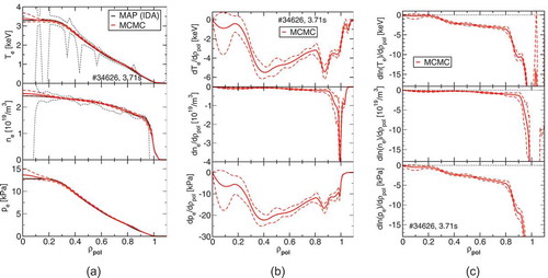
Figure 1 shows as black lines electron temperature, density, and pressure profiles obtained with the MAP approach and an uncertainty band obtained with the ${\chi }^2$-method with a typical profile binning on the order of the diagnostics spatial resolution (Fig. 1a). The uncertainty band depicts the local modification of the profiles where ${\chi }^2$ increased by 1. Since the channel separation of the ECE and TS data is larger than the profile binning chosen, there are spikes in the uncertainty band of the temperature profile. The uncertainty band of the density profile does not show such spikes because the interferometry measurement is a line-integrated diagnostic with five lines of sight (LOSs), one of which approaches the plasma center closely. The oscillating structure in the density uncertainty band arises due to the TS data. The red lines in Fig. 1a depict the mean and standard deviation of the MCMC profile samples. The uncertainty band is much smaller because the full correlation structure of the posterior pdf is intrinsically considered. Furthermore, in contrast to the ${\chi }^2$-method, the sampling is performed within the parameterization scheme using splines. The spline knots for routine analysis are selected nonuniformly to reflect the smoothness of the profiles in the plasma core and to allow for steep gradients at the plasma edge. In this way local profile modifications as used for the ${\chi }^2$-method are excluded resulting in a smaller uncertainty band.

Fig. 1. (a) Profiles of the electron temperature $T_{\mathrm{e}}$, density $n_{\mathrm{e}},$ and pressure $p_{\mathrm{e}}$ profiles; (b) the corresponding gradients with respect to ${\rho }_{\mathrm{p}\mathrm{o}\mathrm{l}}$; and (c) the logarithmic gradient

There is no unambiguous method to estimate an uncertainty band for profiles. The uncertainty of profile estimates and derived quantities is uniquely described with the posterior pdf. Various methods to estimate profile uncertainty bands reflect different properties of the posterior pdf. Therefore, profile uncertainty bands should not be used for UP in modeling codes as they might not reflect the uncertainty of the profile characteristics relevant for modeling. In the case of transport and stability codes, the uncertainty of the profile gradient is relevant. But, the uncertainty of profile gradients cannot be derived easily from the uncertainty band of the profile itself. As mentioned above, the uncertainty band has only incomplete information about the correlation structure. Therefore, a reliable estimation of the gradient uncertainty from this information alone is not only tedious but also in general impossible.

From the MCMC samples of the profiles, the mean and standard deviation of the profile gradients (Fig. 1b) and logarithmic gradients (Fig. 1c) can easily be obtained. Note that the mean of the samples of a logarithmic gradient does not coincide with the ratio of the means of the gradient and of the profile although the difference is typically within the uncertainty. Additionally, the MCMC samples can be used as candidate profiles for a sensitivity study using modeling codes.

Irrespective of the advantages of the MCMC sampling method, a drawback is given by the computation time necessary. A converged MCMC chain requires a large number of samples ($\approx {10}^5$ to ${10}^6$), which results typically in a factor of ${10}^2$ to ${10}^3$ larger computation time compared to the MAP estimation. This makes it less suitable for routine analysis.

III. PROFILE ESTIMATION USING GPR

Gaussian process regression is a popular method for the regression problem where a continuous function $f(x)$ is to be predicted from noisy data $d=f(x)+\epsilon$. Although GPR addresses nonparametric probabilistic modeling of functions, where no explicit form of $f(x)$ is assumed, several assumptions have to be made. The Gaussian process prior, the mean function, the covariance kernel, and hyperparameters describing amplitude and correlation (scale) lengths have to be chosen. Generally, a Gaussian process is used to describe a distribution over functions. Details of GPR can be found in Refs. 6 and 7.

For profile estimation, GPR is beneficial for linear problems, e.g., for interpolation and smoothing of noisy data. For these cases GPR is computationally fast. GPR was chosen for the estimation of ion temperature and velocity profiles at ASDEX Upgrade since these values and their uncertainties are already analyzed from charge exchange recombination spectroscopy (CXRS) measurements.^8,9 The uncertain values have to be regressed, smoothed, interpolated, and extrapolated to the magnetic axis and scrape-off layer (SOL) if no measurements are available in these areas. Since temperature and velocity profiles as a function of magnetic coordinates are expected to have a zero gradient at the plasma center and far in the SOL, the GPR is extended with gradient observations. Assuming that the observed data are $y_{\mathrm{t}}=f(x_{\mathrm{t}})+{\epsilon }_{\mathrm{t}}$ and $y_{\mathrm{p}}^{\prime }=f^{\prime }(x_{\mathrm{p}})+{\epsilon }_{\mathrm{p}}=\frac{df}{dx}|x_{\mathrm{p}}+{\epsilon }_{\mathrm{p}}$ and the newly introduced points, were the profiles to be evaluated (estimated), are ${\mathrm{x}}_{\mathrm{s}}$, the joint multivariate normal distribution of the Gaussian process is

(1) $\left[\begin{array}{c}{y}_{\mathrm{t}}\\ {y^{\prime }}_{\mathrm{p}}\\ f_{\mathrm{s}}\end{array}\right]\sim N\left(0,\left[\begin{array}{cc}{\mathrm{\Sigma }}_{11}& {\mathrm{\Sigma }}_{12}\\ {\mathrm{\Sigma }}_{21}& {\mathrm{\Sigma }}_{22}\end{array}\right]\right),$(1)

(2) ${\mathrm{\Sigma }}_{11}:=\left[\begin{array}{cc}K(x_{\mathrm{t}},x_{\mathrm{t}})+{\sigma }_{\mathrm{t}}^{2}I& \frac{\mathrm{\partial }K(x_{\mathrm{t}},x_{\mathrm{p}})}{\mathrm{\partial }{x}_{\mathrm{p}}}\\ \frac{\mathrm{\partial }K(x_{\mathrm{p}},x_{\mathrm{t}})}{\mathrm{\partial }{x}_{\mathrm{p}}}& \frac{{\mathrm{\partial }}^{2}K(x_{\mathrm{p}},x_{\mathrm{p}})}{\mathrm{\partial }{x}_{\mathrm{p}}\mathrm{\partial }{x}_{\mathrm{p}}}+{\sigma }_{\mathrm{p}}^{2}I\end{array}\right],$(2)

(3) ${\mathrm{\Sigma }}_{12}:=\left[\begin{array}{c}K(x_{\mathrm{t}},x_{\mathrm{s}})\\ \frac{\mathrm{\partial }K(x_{\mathrm{p}},x_{\mathrm{s}})}{\mathrm{\partial }{x}_{\mathrm{p}}}\end{array}\right],$(3)

(4) ${\mathrm{\Sigma }}_{21}:={\left[\begin{array}{c}K(x_{\mathrm{s}},x_{\mathrm{t}})\\ \frac{\mathrm{\partial }K(x_{\mathrm{s}},x_{\mathrm{p}})}{\mathrm{\partial }{x}_{\mathrm{p}}}\end{array}\right]}^T,$(4)

and

(5) ${\mathrm{\Sigma }}_{22}:=\left[\begin{array}{c}K(x_{\mathrm{s}},x_{\mathrm{s}})\end{array}\right],$(5)

where $I$ = identity matrix

${\sigma }_{\mathrm{t}}^2,{\sigma }_{\mathrm{p}}^2$ = variances of the errors ${\epsilon }_{\mathrm{t}}$ and ${\epsilon }_{\mathrm{p}}$,

and where $K(x_1,x_2)$ is the covariance matrix between all observed points $x_{\mathrm{t}}$, $x_{\mathrm{p}}$ and newly introduces points $x_{\mathrm{s}}$. Note that the derivative of the covariance function is taken with respect to the parameter that the derivative points will be plugged in.

The conditional distribution of $f_{\mathrm{s}}=f(x_{\mathrm{s}})$ is normally distributed $f_{\mathrm{s}}\sim N({\bar{f}}_{\mathrm{s}},\mathrm{c}\mathrm{o}\mathrm{v}(f_{\mathrm{s}},f_{\mathrm{s}}))$ with mean

(6) ${\bar{f}}_{\mathrm{s}}={\mathrm{\Sigma }}_{21}{\mathrm{\Sigma }}_{11}^{-1}\left[\begin{array}{c}{y}_{\mathrm{t}}\\ {y^{\prime }}_{\mathrm{p}}\end{array}\right]$(6)

and covariance matrix

(7) $\mathrm{c}\mathrm{o}\mathrm{v}(f_{\mathrm{s}},f_{\mathrm{s}}))={\mathrm{\Sigma }}_{22}-{\mathrm{\Sigma }}_{21}{\mathrm{\Sigma }}_{11}^{-1}{\mathrm{\Sigma }}_{12}.$(7)

Since the matrix ${\mathrm{\Sigma }}_{11}$ is symmetric and positive definite, the mean and covariance can effectively be calculated by employing the Cholesky decomposition.

The joint multivariate normal distribution of the Gaussian process of the observations and the profile gradient $f_{\mathrm{s}}^{\prime }$ is

(8) $\left[\begin{array}{c}{y}_{\mathrm{t}}\\ {y^{\prime }}_{\mathrm{p}}\\ {f^{\prime }}_{\mathrm{s}}\end{array}\right]\sim N\left(0,\left[\begin{array}{cc}{\mathrm{\Sigma }}_{11}& {{\mathrm{\Sigma }}^{\prime }}_{12}\\ {{\mathrm{\Sigma }}^{\prime }}_{21}& {{\mathrm{\Sigma }}^{\prime }}_{22}\end{array}\right]\right),$(8)

(9) ${\mathrm{\Sigma }}_{12}^{\prime }:=\left[\begin{array}{c}\frac{\mathrm{\partial }K(x_{\mathrm{t}},x_{\mathrm{s}})}{\mathrm{\partial }{x}_{\mathrm{s}}}\\ \frac{{\mathrm{\partial }}^{2}K(x_{\mathrm{p}},x_{\mathrm{s}})}{\mathrm{\partial }{x}_{\mathrm{s}}\mathrm{\partial }{x}_{\mathrm{p}}}\end{array}\right],$(9)

(10) ${\mathrm{\Sigma }}_{21}^{\prime }:={\left[\begin{array}{c}\frac{\mathrm{\partial }K(x_{\mathrm{s}},x_{\mathrm{t}})}{\mathrm{\partial }{x}_{\mathrm{s}}}\\ \frac{{\mathrm{\partial }}^{2}K(x_{\mathrm{s}},x_{\mathrm{p}})}{\mathrm{\partial }{x}_{\mathrm{s}}\mathrm{\partial }{x}_{\mathrm{p}}}\end{array}\right]}^T,$(10)

and

(11) ${\mathrm{\Sigma }}_{22}^{\prime }:=\left[\begin{array}{c}\frac{{\mathrm{\partial }}^{2}K(x_{\mathrm{s}},x_{\mathrm{s}})}{\mathrm{\partial }{x}_{\mathrm{s}}\mathrm{\partial }{x}_{\mathrm{s}}}\end{array}\right].$(11)

The conditional distribution of $f_{\mathrm{s}}^{\prime }$ is normally distributed $f_{\mathrm{s}}^{\prime }\sim N(\overline{f_{\mathrm{s}}^{\prime }},\mathrm{c}\mathrm{o}\mathrm{v}(f_{\mathrm{s}}^{\prime },f_{\mathrm{s}}^{\prime }))$ with mean

(12) $\overline{f_{\mathrm{s}}^{\prime }}={\mathrm{\Sigma }}_{21}^{\prime }{\mathrm{\Sigma }}_{11}^{-1}\left[\begin{array}{c}{y}_{\mathrm{t}}\\ {y^{\prime }}_{\mathrm{p}}\end{array}\right]$(12)

and covariance matrix

(13) $\mathrm{c}\mathrm{o}\mathrm{v}(f_{\mathrm{s}}^{\prime },f_{\mathrm{s}}^{\prime }))={\mathrm{\Sigma }}_{22}^{\prime }-{\mathrm{\Sigma }}_{21}^{\prime }{\mathrm{\Sigma }}_{11}^{-1}{\mathrm{\Sigma }}_{12}^{\prime }.$(13)

Candidate profiles for $f_{\mathrm{s}}$ and $f_{\mathrm{s}}^{\prime }$ can be sampled from the corresponding conditional normal distributions.

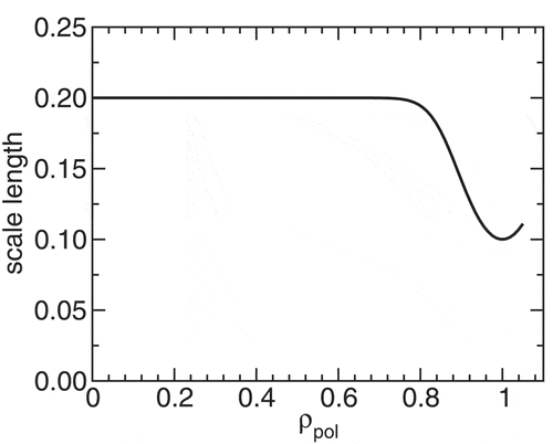
For the reconstruction of kinetic profiles, where different gradient lengths at the plasma core and at the plasma edge occur, nonlocal GPR has to be used, which poses the challenge of selecting different appropriate scale lengths for routine and unsupervised data analyses. Gibbs¹⁰ derived the nonstationary covariance function

(14) $k(x_1,x_2)={\sigma }_f^2\sqrt{\frac{2l(x_1)l(x_2)}{l^2(x_1)+l^2(x_2)}}exp\left(-\frac{{(x_1-x_2)}^2}{l^2(x_1)+l^2(x_2)}\right),$(14)

which is equivalent to the squared exponential covariance function if the length scale is independent of $x$, $l(x)=l.$ The term ${\sigma }_f^2$ is the signal variance, which is typically on the order of the signal amplitude squared to be expected. The length scale $l(x)$ is an arbitrary positive function of $x$.

Similar to the nonstationary scale length in Ref. 7, a hyperbolic tangent was chosen with a core saturation value and a shorter separatrix value to allow for steep edge gradients and a smooth transition in-between:

(15) $l(x)=a\times tanh\left[{\left|\frac{x-x_0}{c}\right|}^{\nu }\right]+b.$(15)

In addition to the four hyperparameters $a$, $b$, $c$, and $x_0$, used in a similar way in Ref. 7, an exponent $\nu$ was introduced to allow for some flexibility in the transition shape. In contrast to Ref. 7, the SOL region has a larger scale length because the largest profile gradients are expected close to the separatrix. Figure 2 shows a realization of the scale-length function with reduced scale length around the separatrix allowing for a steep gradient. The parameters are given by $a=b=0.1$, $c=0.15$, $\nu =2,$ and $x_0=1.0$.

Fig. 2. Scale-length function used for nonstationary GPR

For a refined analysis, the hyperparameters have to be selected in a data-driven way.⁷ The preferred, full-Bayesian approach is given by marginalizing the hyperparameters using a proper prior and an MCMC technique. Since MCMC marginalization can be too expensive for routine analysis, a less elaborate way can be chosen by calculating a point estimate for the hyperparameters applying a maximum likelihood (ML) estimator or a Bayesian MAP estimator including prior information about the hyperparameters.⁷ For the present work, the hyperparameters are selected using a Bayesian MAP estimator because it is observed that a ML estimator might result in oversmoothing or undersmoothing of the data depending on the data coverage. In a routine analysis the data sets typically vary in quality (signal-to-noise ratio) and coverage. For example, if the data coverage is large in regions with small profile curvature, the resulting profile might oversmooth the data in regions with larger profile curvature and less data coverage. Oversmoothing is easily recognized if the residuals do not scatter symmetrically around zero. Therefore, the Bayesian MAP estimator is used with a prior on the hyperparameters, which includes information from scenarios with good data coverage in all profile regions. This prior knowledge about the hyperparameters is supported by typical correlation length scales expected in the plasma core ($\approx 0.2$) and around the last-closed flux surface ($\approx 0.05\mathrm{t}\mathrm{o}0.1$). The physical interpretation of the kernel parameters allows one to provide a plausible range of values for the hyperparameters in the various regions.

Problems might arise with a nonstationary kernel if the change in the length scale is larger than the change in the covariate $x$ (Ref. 10). If the length scale varies too rapidly, then the covariance drops off quite sharply due to the prefactor in Eq. (14)(14) $k(x_1,x_2)={\sigma }_f^2\sqrt{\frac{2l(x_1)l(x_2)}{l^2(x_1)+l^2(x_2)}}exp\left(-\frac{{(x_1-x_2)}^2}{l^2(x_1)+l^2(x_2)}\right),$(14) . This might lead to undesirable profile shapes. In the extreme case of discontinuous scale functions, the sample profiles show a discontinuity where the length scale changes.^7,11 Therefore, the gradient of the length scale is preferred to be $dl/dx<1$.

The estimated profiles, gradient profiles, logarithmic-gradient profiles, and their uncertainties evaluated with this GPR approach (at ASDEX Upgrade referred to as the IDI code) are written into the ASDEX Upgrade database. Figure 3 shows as black dots ion temperatures measured with CXRS. Note that this data set is not representative for the CXRS data at ASDEX Upgrade.⁸ In contrast to the high noise level of the temperatures shown, the CXRS system at ASDEX Upgrade usually provides ion temperatures with much less scatter and uncertainties. The presented data are taken from short beam blips where the signal-to-noise ratio can be small. In addition to that, small signals often suffer from uncertainties in the estimation of the background. This data set was chosen to launch a study about the sensitivity of GENE calculations in a worst-case scenario considering ion profiles.

Fig. 3. (a) Profiles of the measured and estimated ion temperature $T_{\mathrm{i}}$, (b) the corresponding gradient, and (c) the logarithmic gradient

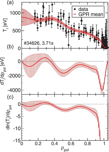
The red lines in Fig. 3 depict the mean and standard deviation of the GPR of the temperature, its gradient, and logarithmic gradient. The profile and its gradient are calculated from the corresponding conditional mean and square root of the covariance diagonal elements, whereas the mean of the logarithmic gradient $f_{\mathrm{s}}^{\prime }/f_{\mathrm{s}}$ and its standard deviation are evaluated from (2000) samples of the conditional distributions of $f_{\mathrm{s}}$ and $f_{\mathrm{s}}^{\prime }$. The large uncertainty of the profile close to the magnetic axis is due to missing data that can only partly be compensated by gradient data. Note that the amplitude in areas without data critically depends on the selection of the hyperparameter ${\sigma }_f$.

The uncertainties of the measured data were validated by reviewing the residuals and the reduced ${\chi }^2/N_{\mathrm{d}\mathrm{a}\mathrm{t}\mathrm{a}}$ value using scenarios with different levels of signal-to-noise ratio. The example depicted in Fig. 3 has a ${\chi }^2/N_{\mathrm{d}\mathrm{a}\mathrm{t}\mathrm{a}}$ value of about 1. A small number of data are about 3σ separated from the fitting curve, which, because of the large number of data, is not appropriate to be interpreted as outliers or misspecification of the uncertainty. Although the signal-to-noise ratio for this example is rather small, the structures in the ion temperature gradient $d{T}_{\mathrm{i}}/d{\rho }_{\mathrm{p}\mathrm{o}\mathrm{l}}$ profiles can also be seen in the electron temperature profile (Fig. 1). The electron temperature is a factor of about 4 larger than $T_{\mathrm{i}}$ but shows a similar flat profile within ${\rho }_{\mathrm{p}\mathrm{o}\mathrm{l}}<0.3$, a steepening within ${\rho }_{\mathrm{p}\mathrm{o}\mathrm{l}}=0.3\mathrm{t}\mathrm{o}0.4,$ and a flattening by nearly a factor of 2 starting at ${\rho }_{\mathrm{p}\mathrm{o}\mathrm{l}}=$0.4 and going until 0.8. Despite the similarities, note that the depicted error margin reflects 1σ only. The structures in the gradient of $T_{\mathrm{i}}$ are on the order of about 3σ, which is also reflected in the samples drawn from the probability distribution.

Figure 4 shows as blue lines candidate profiles by drawing samples from the conditional distributions of $f_{\mathrm{s}}$ and $f_{\mathrm{s}}^{\prime }$. Note that the augmented data with zero gradient at the plasma center (${\rho }_{\mathrm{p}\mathrm{o}\mathrm{l}}=0$) can clearly be seen.

Fig. 4. (a) Candidate profiles of the ion temperature $T_{\mathrm{i}}$, (b) the corresponding gradient, and (c) the logarithmic gradient from sampling the conditional distributions

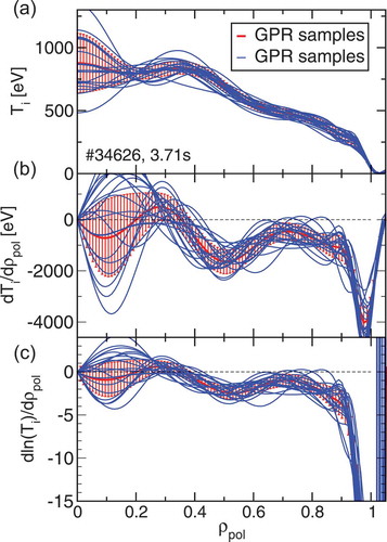
The sampled profiles are only specified by the measured data. No positivity constraint for $T_{\mathrm{i}}$ was applied (although highly desirable). Some samples might disagree with transport modeling (or our physical intuition) especially when the signal-to-noise ratio of the data is small or in regions with missing data. The Bayesian approach allows one to include any kind of information as (uncertain) prior information, e.g., the assumption of a zero gradient at the plasma center. Providing additional information from, e.g., transport modeling, allows one to penalize unphysical results. Frequently, the interpretation of profiles to be unphysical depends on the fidelity of the transport model used. Using only measured data has the advantage to provide a set of profiles not restricted by a model with an uncertainty difficult to be quantified. The Bayesian method allows one to include prior information directly in the GPR or in a second step (GPR being the first step) where the sample distribution is weighted with information from, e.g., transport modeling. The two approaches are equivalent if the measured data and the modeling can be considered to be independent. This assumption is usually valid if the data are not used in the modeling process. The advantages of a multistep approach are that the GPR keeps its analytic solution and different modeling approaches can be tested subsequently.

Figure 5 shows the profiles and profile gradients of the angular velocity $v_{\mathrm{t}\mathrm{o}\mathrm{r}}$ measured with CXRS. Only data from the core CXRS system were used. Data from the edge CXRS system are included as available, which reduces the uncertainties between 0.9 and 1. To have a reasonable transition from the last closed flux surface into the SOL if no reliable data do exist, the $T_{\mathrm{i}}$ or $v_{\mathrm{t}\mathrm{o}\mathrm{r}}$ data can be augmented in the SOL with reasonable (small) values and corresponding large uncertainties (prior information in the SOL). Note that uncertainties in the position of the CXRS measurements are not included in the examples shown. A pragmatic method to consider errors in both coordinates is given by replacing ${\sigma }_{\mathrm{t}}^2$ with ${{ }^{\sim }\sigma }_{\mathrm{t}}^2={\sigma }_{\mathrm{t}}^2+b^2{\sigma }_{\mathrm{p}\mathrm{o}\mathrm{s}}^2,$ where $b$ is the local slope of the profile and ${\sigma }_{\mathrm{p}\mathrm{o}\mathrm{s}}^2$ is the variance of the uncertainty on the position. This example shows the typical uncertainty level for both, ion temperature and velocity measurements at ASDEX Upgrade.

Fig. 5. (a) Profiles of the measured and estimated angular velocity $v_{\mathrm{t}\mathrm{o}\mathrm{r}},$ (b) the corresponding gradient, and (c) the logarithmic gradient

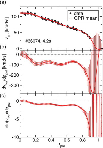
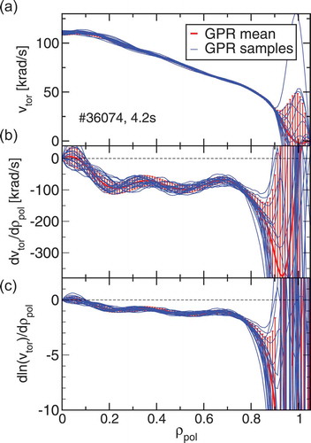
Figure 6 shows as blue lines candidate profiles of $v_{\mathrm{t}\mathrm{o}\mathrm{r}}$ by drawing samples from the conditional distributions. Because of the small uncertainties of the measured data, the scatter of the profiles is much smaller compared to the previous example of the ion temperature.

Fig. 6. (a) Candidate profiles of the angular velocity $v_{\mathrm{t}\mathrm{o}\mathrm{r}},$ (b) the corresponding gradient, and (c) the logarithmic gradient from sampling the conditional distributions

IV. EFFECTIVE ION CHARGE

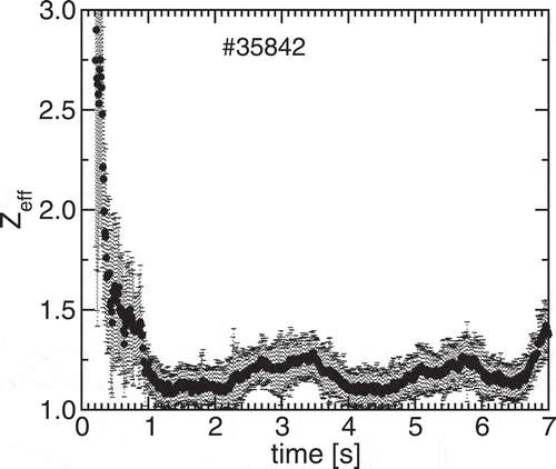
For transport analyses the effective ion charge $Z_{\mathrm{e}\mathrm{f}\mathrm{f}}$ plays a major role. Figure 7 shows $Z_{\mathrm{e}\mathrm{f}\mathrm{f}}$ as a function of time estimated from the bremsstrahlung background of CXRS spectra.¹² Because they are not significantly affected by wall reflections, 5 LOSs out of 25 LOSs were selected. The wall reflection problem is significantly reduced because these LOSs terminate inside of an A-port, opposed to intersecting W limiter surfaces or ion cyclotron range of frequency antennas, although reflections may not be entirely removed. All of the selected LOSs integrate the bremsstrahlung intensity nearly up to the plasma center. Since no spatial resolution is achievable with this LOS setting, a spatially constant $Z_{\mathrm{e}\mathrm{f}\mathrm{f}}$ value is assumed. An extension of the setting with further LOSs not affected by wall reflections for estimating $Z_{\mathrm{e}\mathrm{f}\mathrm{f}}$ profiles is in progress. The uncertainty includes the uncertainty of the bremsstrahlung background and the uncertainties of the temperature and density profiles. The uncertainty of the density profile contributes most to the uncertainty of $Z_{\mathrm{e}\mathrm{f}\mathrm{f}}$ because the bremsstrahlung intensity scales quadratically with the density. Overall, an uncertainty of $Z_{\mathrm{e}\mathrm{f}\mathrm{f}}$ of about 20% is achieved.

Fig. 7. Effective ion charge $Z_{\mathrm{e}\mathrm{f}\mathrm{f}}$ as a function of time including uncertainty

V. MAGNETIC EQUILIBRIUM

For an IDA approach all diagnostics have to be mapped to a magnetic coordinate system, where the electron and ion temperatures and densities are assumed to be constant on flux surfaces. Since the magnetic equilibrium is reconstructed from noisy measurements, uncertain pressure profiles, and uncertain modeling and calibration assumptions, it also suffers from uncertainties. Geometric quantities such as the coordinates of the magnetic axis and the position of the separatrix contour are often uncertain to an extent where it matters for diagnostic or modeling analyses. The uncertainty of equilibrium profiles, e.g., the current density and $q$-profile, are of particular importance to assess the reliability of plasma transport studies.

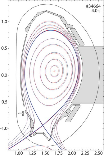
The reliability of equilibrium quantities depends on the coverage of the diagnostic data constraining the equilibrium as well as on the statistical and systematic uncertainty of the individual data. Figure 8 shows contours of the poloidal flux of two equilibria at ASDEX Upgrade evaluated with the CLISTE code¹³ using the standard set of magnetic measurements only and with the recently developed IDE code¹⁴ using additional pressure (kinetic) constraints and current diffusion modeling solving the current diffusion equation (CDE). Details of the analysis of this plasma discharge can be found in Ref. 15. Note that the CLISTE code can also apply kinetic constraints as well as internal measurements from motional Stark effect (MSE) or Faraday rotation measurements. This work shows only CLISTE results obtained using the setting for routine analysis shortly after the plasma discharge using magnetic data only and results using additional pressure (kinetic) constraints. Although the two equilibria appear to be rather similar, there are differences due to the different amount of constraining data and modeling assumptions.

Fig. 8. Poloidal view of magnetic equilibria evaluated with magnetic measurements only (blue) and with additional kinetic constraints and current diffusion modeling (red)

This section shows a selection of examples of equilibrium quantities and their uncertainties as relevant for modeling codes. The chosen examples are not exhaustive. The uncertainties depend on the plasma discharge and time points selected and can vary significantly depending on various parameters, such as if the plasma is in L-mode or H-mode or the calibration precision available for the measurement campaign. The purpose of the examples shown is to give an overview of sources of uncertainty and their typical size at ASDEX Upgrade but should not be interpreted as uncertainties that are always present at this size.

V.A. Scalar Quantities

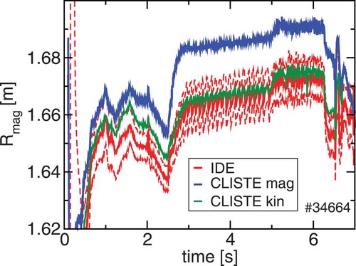
The radial position of the magnetic axis $R_{\mathrm{m}\mathrm{a}\mathrm{g}}$ of the plasma shown in Fig. 8 is depicted in Fig. 9 as a function of time for different evaluations. A reliable estimation of $R_{\mathrm{m}\mathrm{a}\mathrm{g}}$ and of the position of the core flux surfaces is important for profile analysis especially if simultaneous measurements from the low-field side and high-field side are available. If the positions of flux surfaces are erroneously determined, diagnostic data cannot be analyzed uniquely assuming constant quantities on flux surfaces. Additionally, a reliable estimate of $R_{\mathrm{m}\mathrm{a}\mathrm{g}}$ is of utmost importance if MSE measurements have to be analyzed.¹⁵ In the present example, the magnetic axis of the equilibrium using magnetic data only (CLISTE mag) is shifted about 2 cm outward compared to the equilibrium using the extended data and modeling constraints (IDE). The difference in the position of the flux surfaces is mainly due to different reconstructed pressure profiles. In particular, the shape of the pressure profile in the plasma core benefits from kinetic constraints from the sum of thermal electron and ion pressures as well as the fast-ion pressure evaluated, e.g., with the RABBIT code.¹⁶ The improved pressure profile is observed at ASDEX Upgrade to be less peaked applying kinetic constraints, resulting in a smaller Shafranov shift. Even if only thermal pressure constraints are applied at the plasma edge, where no significant contribution from fast ions is expected, the equilibrium pressure profile and the position of the magnetic axis improve (CLISTE kin).

Fig. 9. Comparison of the radial position of the magnetic axis evaluated with magnetic measurements only (CLISTE mag, blue); magnetic and plasma edge thermal pressure (kinetic) constraints (CLISTE kin, green); and with magnetic, full (thermal and fast-ion) pressure constraints and current diffusion modeling (IDE, red lines with upper and lower 1σ uncertainty band)

The uncertainty of the position of the magnetic axis $(R_{\mathrm{m}\mathrm{a}\mathrm{g}},z_{\mathrm{m}\mathrm{a}\mathrm{g}})$ is calculated using

(16) $\mathrm{\Delta }\xi =\sqrt{{\left\{\frac{\mathrm{\partial }\xi }{\mathrm{\partial }{c}_k}\right\}}^{T}C\left\{\frac{\mathrm{\partial }\xi }{\mathrm{\partial }{c}_k}\right\}},$(16)

where $\xi \in (R,z)$. The term $\{c_k\}$ is the set of fitting coefficients of the flux-function basis functions $\{{\psi }_k\}$, where $\psi ={\sum }_k{c}_k{\psi }_k$. The term $C$ is the covariance matrix of the coefficients $\{c_k\}$, $C=(R^T{\mathrm{\Sigma }}^{-1}R{)}^{-1}$, evaluated with the response matrix $R$. The term $R$ links the coefficients with the measurement data $d$, constraining the equilibrium, $\vec{d}=R\vec{c}+\epsilon$. The term $\mathrm{\Sigma }$ is a diagonal matrix with the variances ${\sigma }^2=⟨\mathrm{\Delta }{\epsilon }^2⟩$ on the diagonal. The gradients are calculated using

(17) $\frac{\mathrm{\partial }R}{\mathrm{\partial }{c}_k}=\frac{{\psi }_k{|}_{(R_2,z_{\mathrm{m}\mathrm{a}\mathrm{g}})}-{\psi }_k{|}_{(R_1,z_{\mathrm{m}\mathrm{a}\mathrm{g}})}}{||\mathrm{\nabla }\psi (R_1,z_{\mathrm{m}\mathrm{a}\mathrm{g}})||}$(17)

and

(18) $\frac{\mathrm{\partial }z}{\mathrm{\partial }{c}_k}=\frac{{\psi }_k{|}_{(R_{\mathrm{m}\mathrm{a}\mathrm{g}},z_2)}-{\psi }_k{|}_{(R_{\mathrm{m}\mathrm{a}\mathrm{g}},z_1)}}{||\mathrm{\nabla }\psi (R_{\mathrm{m}\mathrm{a}\mathrm{g}},z_1)||}.$(18)

Since at the magnetic axis $\mathrm{\nabla }\psi (R_{\mathrm{m}\mathrm{a}\mathrm{g}},z_{\mathrm{m}\mathrm{a}\mathrm{g}})=0$, two nearby points on the same flux surface are used with $\psi (R_1,z_{\mathrm{m}\mathrm{a}\mathrm{g}})=\psi (R_2,z_{\mathrm{m}\mathrm{a}\mathrm{g}})$ and $\psi (R_{\mathrm{m}\mathrm{a}\mathrm{g}},z_1)=\psi (R_{\mathrm{m}\mathrm{a}\mathrm{g}},z_2)$.

The 1σ uncertainty of $R_{\mathrm{m}\mathrm{a}\mathrm{g}}$ evaluated with the IDE setting (thin red lines in Fig. 9) is about 6 mm whereas the uncertainty of $R_{\mathrm{m}\mathrm{a}\mathrm{g}}$ using magnetic data only (CLISTE mag) is about 10 mm (not shown). The sawtooth crashes in the time interval 3 to 5 s can clearly be seen in the IDE equilibrium.¹⁵ As with the position of the magnetic axis, the reconstructed plasma energy $W_{\mathrm{m}\mathrm{h}\mathrm{d}}$ also is closely related to the equilibrium pressure profile. The value $W_{\mathrm{m}\mathrm{h}\mathrm{d}}$ of the equilibrium constrained with the kinetic profiles is expected to be more reliable than from magnetic data only. Figure 10 shows the temporal evolution of the $W_{\mathrm{m}\mathrm{h}\mathrm{d}}$ values for the equilibria evaluated with the magnetic measurements only (CLISTE mag, blue); the magnetic and plasma edge thermal pressure (kinetic) constraints (CLISTE kin, green); and with magnetic, full (thermal and fast-ion) pressure constraints and current diffusion modeling (IDE, red). The $W_{\mathrm{m}\mathrm{h}\mathrm{d}}$ values match if pressure constraints are applied (CLISTE kin and IDE). Nevertheless, the internal inductance $l_{\mathrm{i}}$ differs comparing equilibria with (IDE) and without (CLISTE kin) current diffusion modeling. For the two CLISTE equilibria, the quantity ${\beta }_{\mathrm{p}\mathrm{o}\mathrm{l}}+l_{\mathrm{i}}/2$, which is expected to be estimated reliably from magnetic data, agrees because no internal constraints on the current profile are applied (not shown). It is somewhat surprising that the Shafranov shift between the two CLISTE equilibria is different although the ${\beta }_{\mathrm{p}\mathrm{o}\mathrm{l}}+l_{\mathrm{i}}/2$ values are very much the same (not shown). The reason is that in addition to the value of ${\beta }_{\mathrm{p}\mathrm{o}\mathrm{l}}+l_{\mathrm{i}}/2$, the shape of the pressure profile contributes to the Shafranov shift.

Fig. 10. Comparison of the plasma energy $W_{\mathrm{m}\mathrm{h}\mathrm{d}}$ and internal inductance $l_{\mathrm{i}}$ evaluated with magnetic measurements only (CLISTE mag, blue); magnetic and plasma edge thermal pressure (kinetic) constraints (CLISTE kin, green); and with magnetic, full (thermal and fast-ion) pressure constraints and current diffusion modeling (IDE, red)

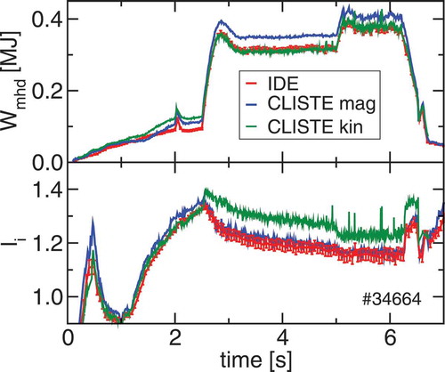
Summarizing, scalar equilibrium quantities, i.e., $R_{\mathrm{m}\mathrm{a}\mathrm{g}}$, $W_{\mathrm{m}\mathrm{h}\mathrm{d}}$, and $l_{\mathrm{i}}$, have not only statistical uncertainties due to measurement noise but also uncertainties depending on the coverage of the diagnostic data constraining the equilibrium and the applied modeling assumptions, e.g., neoclassical current diffusion.

V.B. Profiles

The current and $q$-profiles benefit from internal measurement, i.e., MSE data or Faraday rotation measurements, as well as from current diffusion modeling.¹⁴

Figures 11 and 12 show flux-surface–averaged current density and $q$-profiles evaluated without internal measurements from MSE or Faraday rotation. Only CDE modeling constrains the current profile. The blue and red profiles shown in each of Figs. 11 and 12 are identical as they are both estimated with the same CDE modeling. The only difference is given by the error bars, which are calculated with (red) and without (blue) the CDE modeling constraints. Although for both profiles the current constraints from the CDE are applied, the blue uncertainty bands pretend not to have information from the CDE.

Fig. 11. Current density profile estimated applying constraints from the CDE. The uncertainties are calculated without (blue) and with (red) current constraint included

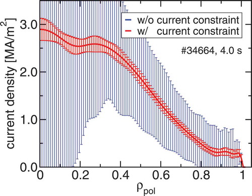
Fig. 12. The $q$-profile estimated applying constraints from the CDE. The uncertainties are calculated without (blue) and with (red) current constraint included

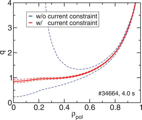
The uncertainty of the current density profile is calculated equivalently to Eq. (16)(16) $\mathrm{\Delta }\xi =\sqrt{{\left\{\frac{\mathrm{\partial }\xi }{\mathrm{\partial }{c}_k}\right\}}^{T}C\left\{\frac{\mathrm{\partial }\xi }{\mathrm{\partial }{c}_k}\right\}},$(16) but using the gradients of the flux-surface–averaged current density with respect to the coefficients. The uncertainty of the $q(=1/\iota )$ values is calculated assuming toroidal flux conservation ${\psi }^{\prime }/\iota ={ }^{\sim }{\psi }^{\prime }{/}^{\sim }\iota$ near the plasma midplane $(R,z_{\mathrm{m}\mathrm{a}\mathrm{g}})$, where ${\psi }^{\prime }=\mathrm{\partial }\psi /\mathrm{\partial }R$ is the true, but unknown, poloidal flux gradient and ${ }^{\sim }{\psi }^{\prime }=\mathrm{\partial }{ }^{\sim }\psi /\mathrm{\partial }R$ is the uncertain equilibrium estimate. From $\mathrm{\Delta }{\psi }^{\prime }:={ }^{\sim }{\psi }^{\prime }-{\psi }^{\prime }={\psi }^{\prime }{(}^{\sim }\iota -\iota )/\iota ={\psi }^{\prime }\mathrm{\Delta }\iota /\iota$ and $\mathrm{\Delta }{\psi }^{\prime }={\sum }_k({ }^{\sim }{c}_k-c_k){{\psi }^{\prime }}_k$, the uncertainty of the rotational transform $\iota$ is obtained by

(19) $\mathrm{\Delta }\iota =\frac{\iota }{{\psi }^{\prime }}\sqrt{{{{\vec{\psi }}^{\prime }}_k}^{T}C{{\vec{\psi }}^{\prime }}_k.}$(19)

The uncertainties in $q$ are asymmetric with $q_{\pm }=1/(\iota \mp \mathrm{\Delta }\iota )$.

In Fig. 12, since no internal measurements are applied, the blue uncertainties increase considerably going from the plasma edge to the plasma core, as expected. The large (blue) uncertainties for both, the current density as well as the $q$-profile, are somewhat surprising because pressure constraints (also known as kinetic constraints) are applied. Since the pressure data only constrain the pressure $p^{\prime }$ term in the Grad-Shafranov equation (GSE) and not the poloidal current $F{F}^{\prime }$ term, the pressure data are not sufficient to regularize the ill-conditioned GSE such that the current density can be inferred.

If the current constraint is applied for the evaluation of the uncertainty, the uncertainty bands become much smaller depending on how much we think the current constraint from neoclassical current diffusion is applicable. Weakening the current constraint results in an increase of the uncertainties on the estimated equilibrium current and $q$-profiles. Nearly independent of how large we select the uncertainty of the current constraint, if no internal current measurements are available, the current constraint determines the estimated current profile because it is the only information available. If other current redistribution mechanisms are present, e.g., by sawtooth reconnection¹⁵ or flux pumping,¹⁷ internal measurements have to be provided to overrule the CDE constraint.

V.C. Separatrix Position

A key quantity for the analysis of data measured at the plasma edge and SOL and for edge modeling is the position of the separatrix contour and its estimation uncertainty. As the separatrix separates the closed flux surfaces from the open field lines, that is, field lines connected to structural components, the transport regime changes significantly. Even small errors in the estimated separatrix position might have significant effects for diagnostic analyses as well as for modeling if steep profile gradients are present.

The analysis of data from various diagnostics often requires an alignment procedure due to uncertainties in the measurement positions as well as due to uncertainties in the equilibrium. For some diagnostics at ASDEX Upgrade, the alignment required between the different diagnostics was observed to be outside of the uncertainties on the measurement locations. Physical criteria such as the separatrix temperature might be employed where the alignment as well as the estimated separatrix temperature itself depends on the separatrix position. Various measurement uncertainties as well as different flexibilities in the equilibrium reconstruction can contribute to the uncertainty of the separatrix position, such as the statistical measurement uncertainty and systematic uncertainty from the calibration of the poloidal field coil arrays; the uncertainties of the currents in the active and passive poloidal field coils; and the modeling of the induced vessel currents.¹⁸

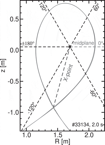
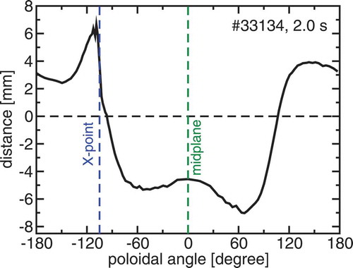
To depict the distance between two separatrix contours, a poloidal coordinate system is introduced unwrapping the last closed flux surface as a function of the poloidal angle. Figure 13 shows two separatrix contours being unwrapped using the poloidal angle fixed at the magnetic axis starting from the outer midplane in counterclockwise direction.

Fig. 13. Separatrix contours and poloidal coordinate system to unwrap the distance of two separatrices

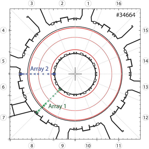
The separatrix position is usually expected to be determined with rather small uncertainties due to the large number ($\approx 50$) of coils measuring the poloidal field close to the plasma. In spite of the small statistical uncertainty of the data ($\approx 1$ mT), the measurement has to be calibrated, which involves systematic uncertainties. Figure 14 shows the toroidal location of two poloidal field coil arrays at ASDEX Upgrade that can be used independently for equilibrium reconstruction.

Fig. 14. Toroidal location of two poloidal field coil arrays

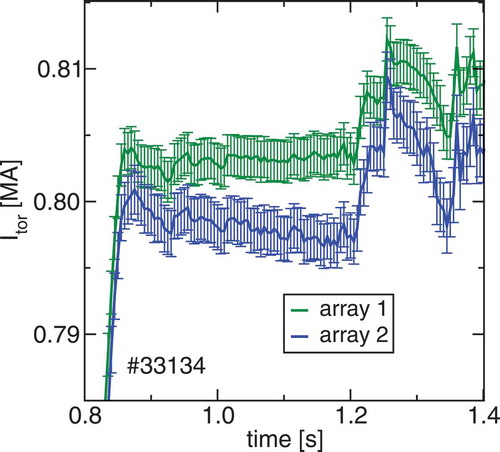
Figure 15 shows the distance between the separatrices (shown in Fig. 13) evaluated with the two poloidal field coil arrays 1 and 2 as a function of the poloidal angle. The separatrix contour estimated with array 2 is nearly everywhere closer to the magnetic axis compared to the separatrix contour estimated with array 1. A sensitivity analysis showed that the difference in the separatrix position could not be associated with shifts in the position of the coil arrays. Consequently, the different separatrix enclosed areas are seen also in the plasma volume (Fig. 16), which is about 1% smaller using array 2 compared to array 1. The same difference of 1% also appears in the reconstructed plasma current (Fig. 17). This 1% deviation in these equilibrium quantities can well be attributed to a systematic calibration uncertainty of about 1%. Current measurements in poloidal field coils are intended to be improved to reduce the calibration uncertainties at ASDEX Upgrade.

Fig. 15. Distance between the separatrices evaluated with either poloidal field coil array 1 or array 2

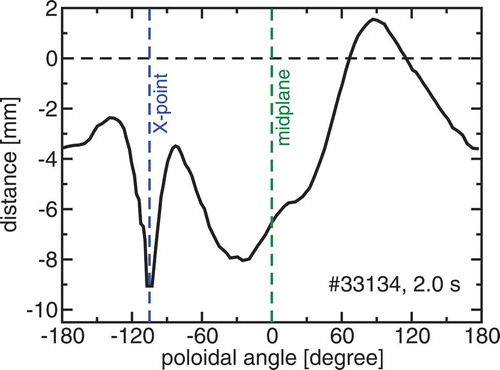
Fig. 16. Temporal evolution of the plasma volume comparing two equilibria using poloidal field array 1 or array 2

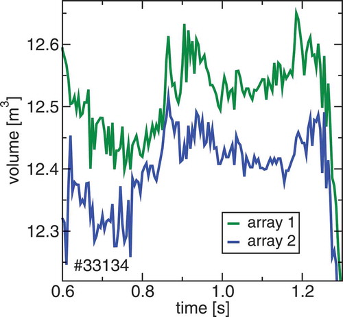
Fig. 17. Temporal evolution of the plasma current comparing two equilibria using poloidal field array 1 or array 2

Another source of uncertainty of the separatrix position arises due to the adjustment of the fitting of the currents in the poloidal field coils. On one hand, the measurements of the currents in the active coils are not known precisely, and on the other hand, there might be induced vessel currents with a poloidal component that might be modeled by fitting coil currents with some flexibility around the measured values. Furthermore, the measurement of the current in the passive stabilization loop (PSL) might be disturbed by toroidally asymmetric PSL currents that might disturb the poloidal field measurements. All of these effects can (partly) be accounted for by relaxing the current in the coils and introducing some flexibility (uncertainty) in the coil currents being fitted together with the equilibrium coefficients. Figure 18 shows the distance between the separatrices evaluated with two different settings: First, use the coil currents as measured, and second, allow some flexibility in the coil currents resulting in an improved fit of the poloidal field measurements. Close to the outer midplane, the separatrix is shifted inward (toward the magnetic axis) by about 5 to 7 mm assuming less flexibility in the coil currents. In contrast, on the high-field side (inner midplane), the separatrix is shifted outward (away from the magnetic axis). The estimated plasma volumes, plasma currents, and plasma energies $W_{\mathrm{m}\mathrm{h}\mathrm{d}}$ are affected only to a minor degree by different flexibilities in the coil current fitting. The only significant effect is a shift of the plasma column in the radial direction. This inward shift is observed to be less consistent with the TS profile diagnostic because it implies to have temperature larger than expected close to the separatrix and in the SOL. Therefore, it is concluded that allowing for some flexibility in the coil current fitting is preferred at ASDEX Upgrade.

Fig. 18. Distance between the separatrices evaluated with less uncertainty in the fitting of the currents in the poloidal field coils compared to allowing for more flexibility to address uncertainties in the current measurements and induced vessel current

VI. SUMMARY

To determine the uncertainty of the results of modeling codes, the uncertainty of various input quantities have to be provided. For the estimation of electron temperature and density profiles and their gradients, MCMC sampling of the posterior pdf of an IDA approach is compared to the frequently used MAP solution. For the estimation of ion temperature and velocity profiles and their gradients, nonstationary GPR is proposed. In addition to the profiles, both methods provide profile gradients, logarithmic gradients, and their uncertainties. Candidate profiles are provided by Monte Carlo sampling. Profile uncertainties can be used for error propagation studies and candidate profiles for sensitivity studies using modeling codes.

The estimation of the uncertainty of various equilibrium quantities is shown. The position and uncertainty of flux surfaces and of the magnetic axis are relevant for the analysis of diagnostics data. The uncertainty of current and $q$-profiles is relevant for uncertainty propagation using plasma transport and stability codes. For plasma edge codes the position of the separatrix contour and its uncertainty at various poloidal positions are of primary interest especially if steep profile gradients are present. Uncertainties in the position of the separatrix contour on the order of 5 mm can be obtained depending on the constraints applied for equilibrium reconstruction as well as depending on the intermittency of the plasma scenario.

Acknowledgments

This work has been carried out within the framework of the EUROfusion Consortium and has received funding from the Euratom research and training programme 2014–2018 and 2019–2020 under grant agreement No. 633053. The views and opinions expressed herein do not necessarily reflect those of the European Commission.

References

- F. JENKO et al., “Electron Temperature Gradient Driven Turbulence,” Phys. Plasmas, 7, 5, 1904 (2000); https://doi.org/10.1063/1.874014.
- S. WIESEN et al., “The New SOLPS-ITER Code Package,” J. Nucl. Mater., 463, 480 (2015); https://doi.org/10.1016/j.jnucmat.2014.10.012.
- R. FISCHER et al., “Probabilistic Lithium Beam Data Analysis,” Plasma Phys. Control. Fusion, 50, 1 (2008); https://doi.org/10.1088/0741-3335/50/8/085009.
- S. S. DENK et al., “Analysis of Electron Cyclotron Emission with Extended Electron Cyclotron Forward Modeling,” Plasma Phys. Control. Fusion, 60, 105010 (2018); https://doi.org/10.1088/1361-6587/aadb2f.
- R. FISCHER et al., “Integrated Data Analysis of Profile Diagnostics at ASDEX Upgrade,” Fusion Sci. Technol., 58, 675 (2010); https://doi.org/10.13182/FST10-110.
- C. E. RASMUSSEN and C. K. I. WILLIAMS, Gaussian Processes for Machine Learning, MIT Press, Cambridge, Massachusetts (2006).
- M. A. CHILENSKI et al., “Improved Profile Fitting and Quantification of Uncertainty in Experimental Measurements of Impurity Transport Coefficients Using Gaussian Process Regression,” Nucl. Fusion, 55, 23012 (2015); https://doi.org/10.1088/0029-5515/55/2/023012.
- E. VIEZZER et al., “High-Resolution Charge Exchange Measurements at ASDEX Upgrade,” Rev. Sci. Instrum., 83, 103501 (2012); https://doi.org/10.1063/1.4755810.
- R. M. McDERMOTT et al., “Extensions to the Charge Exchange Recombination Spectroscopy Diagnostic Suite at ASDEX Upgrade,” Rev. Sci. Instrum., 88, 73508 (2017); https://doi.org/10.1063/1.4993131.
- M. N. GIBBS, “Bayesian Gaussian Processes for Regression and Classification,” PhD Thesis, Cambridge University, Department of Physics (1997).
- S. REECE et al., “Anomaly Detection and Removal Using Non-Stationary Gaussian Processes,” arXiv:1507.00566 [stat.ML] (2015).
- S. K. RATHGEBER et al., “Estimation of Profiles of the Effective Ion Charge at ASDEX Upgrade with Integrated Data Analysis,” Plasma Phys. Control. Fusion, 52, 95008 (2010); https://doi.org/10.1088/0741-3335/52/9/095008.
- P. J. McCARTHY, “Analytical Solutions to the Grad-Shafranov Equation for Tokamak Equilibrium with Dissimilar Source Functions,” Phys. Plasmas, 6, 3554 (1999); https://doi.org/10.1063/1.873630.
- R. FISCHER et al., “Coupling of the Flux Diffusion Equation with the Equilibrium Reconstruction at ASDEX Upgrade,” Fusion Sci. Technol., 69, 526 (2016); https://doi.org/10.13182/FST15-185.
- R. FISCHER et al., “Sawtooth Induced Q-Profile Evolution at ASDEX Upgrade,” Nucl. Fusion, 59, 56010 (2019); https://doi.org/10.1088/1741-4326/ab0b65.
- M. WEILAND et al., “RABBIT: Real-Time Simulation of the NBI Fast-Ion Distribution,” Nucl. Fusion, 58, 82032 (2018); https://doi.org/10.1088/1741-4326/aabf0f.
- I. KREBS et al., “Magnetic Flux Pumping in 3D Nonlinear Magnetohydrodynamic Simulations,” Phys. Plasmas, 24, 102511 (2017); https://doi.org/10.1063/1.4990704.
- J. ILLERHAUS, “Estimation, Validation and Uncertainty of the Position of the Separatrix Contour at ASDEX Upgrade,” IPP 2019-08, Max-Planck-Institut für Plasmaphysik (2019).