A hierarchical asymptotic homogenization approach for viscoelastic composites

Abstract

Effective properties of non-aging linear viscoelastic and hierarchical composites are investigated via a three-scale asymptotic homogenization method. In this approach, we consider the assumption of a generalized periodicity in the different structural levels and their characterization through the so-called stratified functions. The expressions for the associated local and homogenized problems, and the effective coefficients are derived at each level of organization by using the correspondence principle and the Laplace-Carson transform. Considering isotropic components and a perfect contact at the interfaces between the constituents, analytical solutions, in the Laplace-Carson space, are found for the local problems and the effective coefficients are computed. An interconversion procedure between the effective relaxation modulus and the effective creep compliance is carried out for obtaining information about both viscoelastic properties. The numerical inversion to the original temporal space is also performed. Finally, we exploit the potential of the approach and study the overall properties of a hierarchical viscoelastic composite structure representing the dermis.

Keywords:

• Dermis
• hierarchical structures
• viscoelastic composites
• non-aging
• three-scale asymptotic homogenization method
• generalized periodicity

1. Introduction

In the scientific literature there exist several works focusing on the development of micromechanical techniques to predict the macroscopic properties of composite materials. An excellent review on these methods can be found in Sevostianov and Giraud [1]; Davit et al. [2]. In particular, multiscale asymptotic homogenization methods take advantage of the information available at the smaller scales of a given heterogeneous medium to predict the effective properties at its larger scales (see e.g. Lukkassen and Milton [3]; Penta and Gerisch [4]; Ramírez-Torres et al. [5]; Ramírez-Torres et al. [6]; Yang et al. [7]; Dong et al. [8]). This homogenization procedure requires the solution of cell problems with input data corresponding to the homogenized material properties resulting in previous steps. In addition, the use of more general periodic or stratification functions (see e.g. Tsalis, Chatzigeorgiou, and Charalambakis [9]; Tsalis et al. [10]) permits to describe the different length scales of the composite materials. They can be applied to homogenization problems related to hierarchical real-world composites as human tissue (see e.g. Penta et al. [11] for bone and tendons) that generally form geometries which cannot be produced by the repetition of one elementary volume.

In the present work, the three-scale Asymptotic Homogenization Method (AHM) introduced in Ramírez-Torres et al. [5]; Ramírez-Torres et al. [6]; Ramírez-Torres et al. [12] is used to model a non-aging linear viscoelastic composite material with generalized periodicity and two hierarchical levels. This three-scale asymptotic approach has been used for modeling hierarchical laminated and fiber-reinforced elastic composites in Ramírez-Torres et al. [5] and Ramírez-Torres et al. [6]; Ramírez-Torres et al. [12], respectively. Also, there are several other works dealing with the modeling of multiscale hierarchical heterogeneous media. For example, from the theoretical point of view we find the works Allaire and Briane [13]; Bensoussan, Papanicolau, and Lions [14]; Trucu, Chaplain, and Marciniak-Czochra [15]. Regarding these results, a rigorous study about the multiscale convergence is developed in Bensoussan, Papanicolau, and Lions [14]; here the authors consider that $y=x/\epsilon$ and $z=x/{\epsilon }^2$ are the local variables. Subsequently, and applied to the heat equation for composites, the method of reiterate homogenization is well founded in Allaire and Briane [13]. An additional overview of reiterated homogenization is presented in Trucu, Chaplain, and Marciniak-Czochra [15] via a three-scale convergence approach where the asymptotic parameters independently approach zero. More recently, in Dong et al. [8]; Yang et al. [7, 16], the authors study the properties of thermo-mechanical, non-aging and aging viscoelastic composites with multiple spatial scales by using a three-scale asymptotic expansion and a periodic layout of the heterogeneities in the structures. They also provide a finite element algorithm based on inverse Laplace transform and the three-scale asymptotic homogenization to obtain the numerical results.

The article presents some novelties with respect to previous works of ours [5, 17] and, to the best of our knowledge, with others in the literature [7, 16, 18–20]). Specifically, we generalize the results obtained in [5] for linear elasticity by extending them to a non-aging, linear viscoelasticity framework; we deal with the stratified functions in the homogenization procedure; an analytical solution for the local problems associated with each hierarchical level is obtained; the expressions for the effective coefficients for hierarchical laminated composites with generalized periodicity, isotropic components and perfect contact at the interfaces are provided; and the methodology is used to model the overall behavior of the dermis in the skin. A better understanding of this tissue has a real impact on biomedical applications and in the development of modern technology such as flexible instance electronics, soft robotics and prosthetics (see Ref. [21]). Many researches are focused on the study of the viscoelastic, non-linear hyperelastic and anisotropic behavior of the structural components of the skin (see Ref. [22, 23]) and the relation with its hierarchical structure (see Ref. [21, 24]). An inherent characteristic of the mechanical properties of the skin lies in the fact that its properties vary according to the skin type, age, gender, location, and other environmental factors Panchal et al. [25]. In particular, skin has three main layers: the epidermis, the dermis and the hypodermis, in addition to the stratum corneum that acts as the outermost barrier of human skin Muha et al. [26]. Our research is focused on the dermis which represents the most important mechanical and thermal unit of the skin, as it occupies around 90% of the skin’s thickness (see Ref. [27]). In the present work, the dermis is assumed to behave as a non-aging linear viscoelastic and hierarchical composite material, and thus, the investigation of its effective properties is based on the correspondence principle and the Laplace transform (see Ref. [28]). The procedure, see for instance To et al. [29] and Yang et al. [16], consists in the change of the convolution constitutive law by a fictitious elastic one in the Laplace domain. Then, the inversion of the Laplace transform is considered to derive the effective behavior in the time domain.

The article is organized as follows. The mathematical framework of the problem and the homogenization steps are illustrated in Sections 2 and 3, respectively. In Section 4, we present the analytical solution of the local problems and the calculation of the effective coefficients. In Section 5, we highlight the potential of the current approach in the investigation of the effective relaxation and creep compliance properties of the dermis.

2. The linear viscoelastic problem for hierarchical structures

2.1. Separation of scales

Let us consider the dimensionless, scaling parameters ${\epsilon }_1$ and ${\epsilon }_2,$ defined as follows, (see Ref. [12]) (1) $${\epsilon }_1:=\frac{{\ell }_1}{L}\ll 1\hspace{1em}\text{and}\hspace{1em}{\epsilon }_2:=\frac{{\ell }_2}{L}\ll {\epsilon }_1.$$(1)

In addition, the well-separated characteristic length scales ${\ell }_1,{\ell }_2$ and L introduce three dimensionless spatial variables in the reference configuration, (2) $$\overline{x}:=\frac{x}{L},\hspace{1em}\overline{y}:=\frac{x}{{\ell }_1}\hspace{1em}\text{and}\hspace{1em}\overline{z}:=\frac{x}{{\ell }_2},$$(2) where x is said to be the physical spatial variable, whereas $\overline{x},\overline{y}$ and $\overline{z}$ represent the macroscopic, mesoscopic and the microscopic dimensionless spatial variables, respectively.

By using Eq. (1(1) $${\epsilon }_1:=\frac{{\ell }_1}{L}\ll 1\hspace{1em}\text{and}\hspace{1em}{\epsilon }_2:=\frac{{\ell }_2}{L}\ll {\epsilon }_1.$$(1) ), $\overline{x},\overline{y}$ and $\overline{z}$ can be related through the expressions, (3) $$\overline{y}=\frac{x}{{\ell }_1}=\frac{x/L}{{\ell }_1/L}=\frac{\overline{x}}{{\epsilon }_1},$$(3) (4) $$\overline{z}=\frac{x}{{\ell }_2}=\frac{x/L}{{\ell }_2/L}=\frac{\overline{x}}{{\epsilon }_2}.$$(4)

Now, by defining a field $\varphi$ over the region of interest, the separation of scales allows to rephrase the space dependence of $\varphi$ as $\varphi (x)=\check{\varphi }(\overline{x}(x),\overline{y}(x),\overline{z}(x)),$ and taking into account Eqs. (1)–(4), the spatial derivative of $\varphi$ can be computed as follows, (5) $$\begin{array}{c}\frac{\partial {\varphi }_i}{\partial x_j}=\frac{1}{L}\frac{\partial {\check{\varphi }}_i}{\partial {\overline{x}}_j}+\frac{1}{{\ell }_1}\frac{\partial {\check{\varphi }}_i}{\partial {\overline{y}}_n}+\frac{1}{{\ell }_2}\frac{\partial {\check{\varphi }}_i}{\partial {\overline{z}}_m},\\ =\frac{1}{L}\left[\frac{\partial {\check{\varphi }}_i}{\partial {\overline{x}}_j}+\frac{1}{{\epsilon }_1}\frac{\partial {\check{\varphi }}_i}{\partial {\overline{y}}_n}+\frac{1}{{\epsilon }_2}\frac{\partial {\check{\varphi }}_i}{\partial {\overline{z}}_m}\right].\end{array}$$(5)

In the present work, we consider the generalized periodicity (see Ref. [9, 10]) as an additional condition in our model, and thus, we rewrite the three dimensionless spatial variables in Eq. (2(2) $$\overline{x}:=\frac{x}{L},\hspace{1em}\overline{y}:=\frac{x}{{\ell }_1}\hspace{1em}\text{and}\hspace{1em}\overline{z}:=\frac{x}{{\ell }_2},$$(2) ) as follows (6) $$\overline{x}:=\frac{x}{L},\hspace{1em}\overline{y}:=\frac{{\rho }^{(y)}(x)}{{\ell }_1}\hspace{1em}\text{and}\hspace{1em}\overline{z}:=\frac{{\rho }^{(z)}(x)}{{\ell }_2},$$(6) where ${\rho }^{(\alpha )}:{\mathbb{R}}^3\to {\mathbb{R}}^3,$ with $\alpha =y,z$ and the property ${\rho }^{(\alpha )}\in C^{\infty }(\Omega ),$ represent the so-called stratified functions. It is worthy to note that the parametric equations ${\rho }^{(\alpha )}(x)=\text{constant},$ describe the structural organization of the constituents at the ${\epsilon }_1$ and ${\epsilon }_2$ hierarchical levels, respectively.

Therefore, we have that (7) $$\overline{y}=\frac{{\rho }^{(y)}(x)}{{\ell }_1}=\frac{{\rho }^{(y)}(x)/L}{{\ell }_1/L}=\frac{{\overline{\rho }}^{(y)}(x)}{{\epsilon }_1},$$(7) (8) $$\overline{z}=\frac{{\rho }^{(z)}(x)}{{\ell }_2}=\frac{{\rho }^{(z)}(x)/L}{{\ell }_2/L}=\frac{{\overline{\rho }}^{(z)}(x)}{{\epsilon }_2}.$$(8)

In addition, the spatial derivative of $\varphi$ is given by the formula (9) $$\frac{\partial {\varphi }_i}{\partial x_j}=\frac{1}{L}\left[\frac{\partial {\check{\varphi }}_i}{\partial {\overline{x}}_j}+\frac{1}{{\epsilon }_1}\frac{\partial {\check{\varphi }}_i}{\partial {\overline{y}}_n}\frac{\partial {\rho }_n^{(y)}}{\partial x_j}+\frac{1}{{\epsilon }_2}\frac{\partial {\check{\varphi }}_i}{\partial {\overline{z}}_m}\frac{\partial {\rho }_m^{(z)}}{\partial x_j}\right].$$(9)

By following this approach, all equations should be written in dimensionless form. In the literature, the switch to auxiliary variables $\overline{x},\overline{y}$ and $\overline{z}$ is often omitted. However, as shown for example in Auriault, Boutin, and Geindreau [30], both paths are equivalent. Therefore, in the article, the analysis is carried out directly in a system of physical variables x, y and z, where (10) $$y=\frac{{\rho }^{(y)}(x)}{{\epsilon }_1}\hspace{1em}\text{and}\hspace{1em}z=\frac{{\rho }^{(z)}(x)}{{\epsilon }_2}.$$(10)

Similar ideas are developed in Ramírez-Torres et al. [31] to the case of two scales.

2.2. The physical model

Let us denote by $\Omega \in {\mathbb{R}}^3$ a linear multiscale viscoelastic composite material (see Figure 1) characterized by a generalized periodicity at the different levels of organization.

Figure 1. (a) Macroscale: viscoelastic heterogeneous material. (b) ${\epsilon }_1$-structural level. Mesoscale: quasi-periodic cell. (c) ${\epsilon }_2$-structural level. Microscale: quasi-periodic cell. The inclusions do not intersect the boundaries.

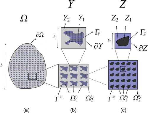
First stage: ${\epsilon }_1$-structural level:

The domain Ω is considered to be a two-phase quasi-periodic composite such that $\overline{\Omega }={\overline{\Omega }}_1^{{\epsilon }_1}\cup {\overline{\Omega }}_2^{{\epsilon }_1}$ and ${\overline{\Omega }}_1^{{\epsilon }_1}\cap {\Omega }_2^{{\epsilon }_1}={\Omega }_1^{{\epsilon }_1}\cap {\overline{\Omega }}_2^{{\epsilon }_1}=\varnothing$ (see Figure 1(b)). It is assumed that ${\Omega }_1^{{\epsilon }_1}={\cup }_{i=1}^{N_1}{}_i{\Omega }_1^{{\epsilon }_1},$ where N₁ denotes the number of inclusions, and we denote with ${\Gamma }^{{\epsilon }_1}$ the interface between ${\Omega }_1^{{\epsilon }_1}$ and ${\Omega }_2^{{\epsilon }_1}.$ In this description, Y represents the unitary periodic cell and the its constituents fulfill the constraint $\overline{Y}={\overline{Y}}_1\cup {\overline{Y}}_2$ and ${\overline{Y}}_1\cap Y_2=Y_1\cap {\overline{Y}}_2=\varnothing .$ The interface between Y₁ and Y₂ is denoted with Γ_Y.

Second stage: ${\epsilon }_2$-structural level

At this structural level we consider that, at the same time, each phase ${}_i{\Omega }_1^{{\epsilon }_1}$ ($i=1,\dots ,N_1$) is a two-phase quasi-periodic composite material, where ${}_i{\overline{\Omega }}_1^{{\epsilon }_1}={\overline{\Omega }}_1^{{\epsilon }_2}\cup {\overline{\Omega }}_2^{{\epsilon }_2}$ and ${\overline{\Omega }}_1^{{\epsilon }_2}\cap {\Omega }_2^{{\epsilon }_2}={\Omega }_1^{{\epsilon }_2}\cap {\overline{\Omega }}_2^{{\epsilon }_2}=\varnothing$ (see Figure 1(c)). Besides, ${\Omega }_1^{{\epsilon }_2}={\cup }_{j=1}^{N_2}{}_j{\Omega }_1^{{\epsilon }_2}$ and ${\Gamma }^{{\epsilon }_2}$ represents the interface between ${\Omega }_1^{{\epsilon }_2}$ and ${\Omega }_2^{{\epsilon }_2}.$ Besides, Z is the corresponding unitary periodic cell, in which we enforce that the constituents satisfy the following relation $\overline{Z}={\overline{Z}}_1\cup {\overline{Z}}_2$ and ${\overline{Z}}_1\cap Z_2=Z_1\cap {\overline{Z}}_2=\varnothing .$ The interface between Z₁ and Z₂ is indicated with Γ_Z.

At this point, we extend the concept of generalized or quasi-periodicity, given in Tsalis, Chatzigeorgiou, and Charalambakis [9]; Tsalis et al. [10], to the case of hierarchical composites with three scales. The definition is presented as follows,

Definition 2.1.

(Generalized periodicity) A composite material with two structural levels of organization is said to have generalized periodicity (or quasi-periodicity) if there exists a global spatial coordinate system x and functions ${\rho }^{(\alpha )}:{\mathbb{R}}^3\to {\mathbb{R}}^3,$ with $\alpha =y,z$ (see Eq. (10(10) $$y=\frac{{\rho }^{(y)}(x)}{{\epsilon }_1}\hspace{1em}\text{and}\hspace{1em}z=\frac{{\rho }^{(z)}(x)}{{\epsilon }_2}.$$(10) )) such that the operator $\mathcal{F}$ which relates the second-order stress tensor $\mathit{\sigma }$ and the second-order strain tensor $\mathit{\xi },$ by the relation $$\mathit{\sigma }=\mathcal{F}(\mathit{\xi };x,y,z),$$ is regular in x, and periodic in y and z.

This concept will permit us to study different structural effects in the composite.

Remark 1.

From now on, we consider the following notation ${\varphi }^{\epsilon }(x,t)=\varphi (x,y,z,t),$ where ${\varphi }^{\epsilon }$ is assumed to be periodic in y and z.

2.3. Formulation of the problem

Considering that the constitutive response of all the constituents of the composite body is linear viscoelastic, and ignoring inertial terms, the problem in Ω reads, (11a) $$\nabla ·{\mathit{\sigma }}^{\epsilon }(x,t)+\mathit{f}(x,t)=\mathbf{0}\text{in}\Omega \setminus ({\Gamma }^{{\epsilon }_1}\cup {\Gamma }^{{\epsilon }_2})\times \mathbb{R},$$(11a) (11b) $${\mathit{u}}^{\epsilon }(x,t)=\overline{\mathit{u}}\text{on}\partial {\Omega }_d\times \mathbb{R},$$(11b) (11c) $${\mathit{\sigma }}^{\epsilon }(x,t)·\mathit{n}=\overline{\mathit{S}}\text{on}\partial {\Omega }_n\times \mathbb{R},$$(11c) (11d) $${\mathit{u}}^{\epsilon }(x,t)=\mathbf{0}\text{in}\Omega \times \left\{0\right\},$$(11d) where, by taking into account Definition 1, $\mathit{\sigma }$ is given by the following scale-dependent constitutive law (see Ref. [32]), (12) $${\mathit{\sigma }}^{\epsilon }(x,t)=\underset{0}{\overset{t}{\int }}{\mathcal{R}}^{\epsilon }(x,t-\tau ):\frac{\partial \mathit{\xi }({\mathit{u}}^{\epsilon }(x,\tau ))}{\partial \tau }d\tau .$$(12)

In Eq. (12(12) $${\mathit{\sigma }}^{\epsilon }(x,t)=\underset{0}{\overset{t}{\int }}{\mathcal{R}}^{\epsilon }(x,t-\tau ):\frac{\partial \mathit{\xi }({\mathit{u}}^{\epsilon }(x,\tau ))}{\partial \tau }d\tau .$$(12) ), $\mathit{\xi }$ denotes the second-order strain tensor determined by the formula (13) $$\mathit{\xi }\left({\mathit{u}}^{\epsilon }(x,t)\right)=\frac{1}{2}\left(\nabla {\mathit{u}}^{\epsilon }(x,t)+{(\nabla {\mathit{u}}^{\epsilon }(x,t))}^T\right),$$(13) and u is the displacement field. Moreover, f denotes the action of external volume forces that satisfies $\mathit{f}(x,t)\in L^2(\Omega \times \mathbb{R}),\overline{\mathit{u}}$ and $\overline{\mathit{S}}$ are the prescribed displacement and traction on the boundary $\partial \Omega =\partial {\Omega }_d\cup \partial {\Omega }_n,$ with $\partial {\Omega }_d\cap \partial {\Omega }_n=\varnothing$ and n is the outward unit vector normal to the surface $\partial \Omega .$ The relaxation modulus is denoted by ${\mathcal{R}}^{\epsilon }$ with the following symmetry properties ${\mathcal{R}}_{\mathit{ijkl}}^{\epsilon }={\mathcal{R}}_{\mathit{jikl}}^{\epsilon }={\mathcal{R}}_{\mathit{ijlk}}^{\epsilon }={\mathcal{R}}_{\mathit{klij}}^{\epsilon }.$ Furthermore, we assume that ${\mathcal{R}}^{\epsilon }\in L^{\infty }(\Omega \times \mathbb{R})$ and that it is positively defined, i.e. the relation ${\mathcal{R}}_{\mathit{ijkl}}^{\epsilon }{\eta }_{ij}{\eta }_{kl}\ge \beta {\eta }^{ij}{\eta }^{kl}$ is verified for all symmetric real valued second-order tensors $\mathit{\eta }$ and some positive constant β.

We further impose continuity conditions for displacements and tractions on both ${\Gamma }^{{\epsilon }_1}$ and ${\Gamma }^{{\epsilon }_2},$ i.e. (14) $$⟦{\mathit{u}}^{\epsilon }(x,t)⟧=\mathbf{0},\hspace{1em}⟦{\mathit{\sigma }}^{\epsilon }(x,t)·{\mathit{n}}^{(\alpha )}⟧=\mathbf{0},\hspace{1em}(\alpha =y,z),$$(14) where the outward unit vectors to the surfaces ${\Gamma }^{{\epsilon }_1}$ and ${\Gamma }^{{\epsilon }_2}$ are represented by ${\mathit{n}}^{(y)}$ and ${\mathit{n}}^{(z)},$ respectively. The operator $⟦{\varphi }^{\epsilon }⟧$ denotes the “jump” of ${\varphi }^{\epsilon }$ across the interface between the constituents.

2.4. Re-formulation of the problem in Laplace-Carson space

The scale-dependent constitutive law Eq. (12(12) $${\mathit{\sigma }}^{\epsilon }(x,t)=\underset{0}{\overset{t}{\int }}{\mathcal{R}}^{\epsilon }(x,t-\tau ):\frac{\partial \mathit{\xi }({\mathit{u}}^{\epsilon }(x,\tau ))}{\partial \tau }d\tau .$$(12) ) corresponds to the special form of a non-aging linear viscoelastic materials where we emphasize the specific functional dependency on $t-\tau$ (see Ref. [33]). Therefore, the viscoelastic problem given by Eqs. (11a–14) can be transformed into an elastic one using the Laplace-Carson transform. It is defined for all real numbers $t\ge 0$ as (see Appendix B in Christensen [32]) $${\varphi }^{\epsilon }(x,p)=p{\int }_0^{\infty }{e}^{-pt}{\varphi }^{\epsilon }(x,t)dt,$$ where the variable p denotes the Laplace-Carson space.

The aforementioned transformation is known as the correspondence principle and permits us to rewrite the system Eqs. (11a–11d) in the Laplace-Carson space, (15a) $$\nabla ·\left[{\mathcal{R}}^{\epsilon }\left(x,p\right):\mathit{\xi }\left({\mathit{u}}^{\epsilon }\left(x,p\right)\right)\right]+\mathit{f}(x,p)=\mathbf{0},\text{in}(\Omega \setminus ({\Gamma }^{{\epsilon }_1}\cup {\Gamma }^{{\epsilon }_2}))\times [0,+\infty ),$$(15a) (15b) $${\mathit{u}}^{\epsilon }\left(x,p\right)=\overline{\mathit{u}}\text{on}\partial {\Omega }_d\times [0,+\infty ),$$(15b) (15c) $${\mathcal{R}}^{\epsilon }\left(x,p\right):\mathit{\xi }\left({\mathit{u}}^{\epsilon }\left(x,p\right)\right)·\mathit{n}=\overline{\mathit{S}}\text{on}\partial {\Omega }_n\times [0,+\infty ),$$(15c) (15d) $${\mathit{u}}^{\epsilon }(x,p)=\mathbf{0}\text{in}\Omega \times \left\{0\right\}.$$(15d)

Furthermore, the interface contact conditions become, (16) $$⟦{\mathit{u}}^{\epsilon }(x,p)⟧=\mathbf{0},\hspace{1em}⟦{\mathcal{R}}^{\epsilon }\left(x,p\right):\mathit{\xi }\left({\mathit{u}}^{\epsilon }\left(x,p\right)\right)·{\mathit{n}}^{(\alpha )}⟧=\mathbf{0}\hspace{1em}\left(\alpha =y,z\right).$$(16)

Remark 2.

In what follows the functions depending on the variable p (e.g. ${\varphi }^{\epsilon }(x,p)$) are defined in the Laplace-Carson space and the homogenization process is developed in Laplace-Carson space.

3. The three-scale asymptotic homogenization approach

In this section we recall the three-scale asymptotic homogenization approach introduced in Ramírez-Torres et al. [5] and we adapt it to the investigation of the overall behavior of hierarchical, linear viscoelastic composites with generalized periodicity of its internal structure.

We first notice that, since each field and material property ${\varphi }^{\epsilon }(x,p)$ are assumed to be regular in x and periodic in y and z, the separation of scales together with Eq. (10(10) $$y=\frac{{\rho }^{(y)}(x)}{{\epsilon }_1}\hspace{1em}\text{and}\hspace{1em}z=\frac{{\rho }^{(z)}(x)}{{\epsilon }_2}.$$(10) ) imply that, (17) $$\frac{\partial {\varphi }_i{}^{\epsilon }\left(x,p\right)}{\partial x_j}=\frac{\partial {\varphi }_i\left(x,y,z,p\right)}{\partial x_j}+\frac{1}{{\epsilon }_1}\frac{\partial {\rho }_n^{\left(y\right)}\left(x\right)}{\partial x_j}\frac{\partial {\varphi }_i\left(x,y,z,p\right)}{\partial y_n}+\frac{1}{{\epsilon }_2}\frac{\partial {\rho }_m^{\left(z\right)}\left(x\right)}{\partial x_j}\frac{\partial {\varphi }_i\left(x,y,z,p\right)}{\partial z_m},$$(17) and using a similar idea, the Eq. (13)(13) $$\mathit{\xi }\left({\mathit{u}}^{\epsilon }(x,t)\right)=\frac{1}{2}\left(\nabla {\mathit{u}}^{\epsilon }(x,t)+{(\nabla {\mathit{u}}^{\epsilon }(x,t))}^T\right),$$(13) becomes, (18) $${\xi }_{kl}\left({\varphi }^{\epsilon }\left(x,p\right)\right)={\xi }_{kl}\left(\varphi \left(x,y,z,p\right)\right)+\frac{1}{{\epsilon }_1}{\xi }_{kl}^{(y)}\left(\varphi \left(x,y,z,p\right)\right)+\frac{1}{{\epsilon }_2}{\xi }_{kl}^{(z)}\left(\varphi \left(x,y,z,p\right)\right),$$(18) where (19a) $${\xi }_{kl}^{(y)}\left(\varphi \left(x,y,z,p\right)\right)=\frac{1}{2}\frac{\partial }{\partial y_m}(\frac{\partial {\rho }_m^{\left(y\right)}(x)}{\partial x_l}{\varphi }_k\left(x,y,z,p\right)+\frac{\partial {\rho }_m^{\left(y\right)}(x)}{\partial x_k}{\varphi }_l\left(x,y,z,p\right)),$$(19a) (19b) $${\xi }_{kl}^{(z)}\left(\varphi \left(x,y,z,p\right)\right)=\frac{1}{2}\frac{\partial }{\partial z_n}(\frac{\partial {\rho }_n^{\left(z\right)}(x)}{\partial x_l}{\varphi }_k\left(x,y,z,p\right)+\frac{\partial {\rho }_n^{\left(z\right)}(x)}{\partial x_k}{\varphi }_l\left(x,y,z,p\right)).$$(19b)

3.1. Three-scale homogenization procedure

Following Ramírez-Torres et al. [5], the solution to the problem Eqs. (15a–16) is given as follows, (20) $${\mathit{u}}^{\epsilon }\left(x,p\right)={\tilde{\mathit{u}}}^{\left(0\right)}\left(x,y,z,p\right)+\sum _{i=1}^{+\infty }{\tilde{\mathit{u}}}^{(i)}\left(x,y,z,p\right){\epsilon }_2^i,$$(20) where ${\tilde{\mathit{u}}}^{(0)}$ is defined as (21) $${\tilde{\mathit{u}}}^{\left(0\right)}\left(x,y,z,p\right)={\mathit{u}}^{\left(0\right)}\left(x,y,z,p\right)+\sum _{i=1}^{+\infty }{\mathit{u}}^{\left(i\right)}\left(x,y,z,p\right){\epsilon }_1^i.$$(21)

Here and subsequently (unless necessary), the variable dependence is dropped out for convenience.

Replacing expansion Eq. (20(20) $${\mathit{u}}^{\epsilon }\left(x,p\right)={\tilde{\mathit{u}}}^{\left(0\right)}\left(x,y,z,p\right)+\sum _{i=1}^{+\infty }{\tilde{\mathit{u}}}^{(i)}\left(x,y,z,p\right){\epsilon }_2^i,$$(20) ) into Eq. (15a(15a) $$\nabla ·\left[{\mathcal{R}}^{\epsilon }\left(x,p\right):\mathit{\xi }\left({\mathit{u}}^{\epsilon }\left(x,p\right)\right)\right]+\mathit{f}(x,p)=\mathbf{0},\text{in}(\Omega \setminus ({\Gamma }^{{\epsilon }_1}\cup {\Gamma }^{{\epsilon }_2}))\times [0,+\infty ),$$(15a) ) and using the relations Eqs. (17(17) $$\frac{\partial {\varphi }_i{}^{\epsilon }\left(x,p\right)}{\partial x_j}=\frac{\partial {\varphi }_i\left(x,y,z,p\right)}{\partial x_j}+\frac{1}{{\epsilon }_1}\frac{\partial {\rho }_n^{\left(y\right)}\left(x\right)}{\partial x_j}\frac{\partial {\varphi }_i\left(x,y,z,p\right)}{\partial y_n}+\frac{1}{{\epsilon }_2}\frac{\partial {\rho }_m^{\left(z\right)}\left(x\right)}{\partial x_j}\frac{\partial {\varphi }_i\left(x,y,z,p\right)}{\partial z_m},$$(17) ) and (18(18) $${\xi }_{kl}\left({\varphi }^{\epsilon }\left(x,p\right)\right)={\xi }_{kl}\left(\varphi \left(x,y,z,p\right)\right)+\frac{1}{{\epsilon }_1}{\xi }_{kl}^{(y)}\left(\varphi \left(x,y,z,p\right)\right)+\frac{1}{{\epsilon }_2}{\xi }_{kl}^{(z)}\left(\varphi \left(x,y,z,p\right)\right),$$(18) ), it is obtained (22) $$\begin{array}{c}\frac{\partial }{\partial x_j}\left[{\mathcal{R}}_{\mathit{ijkl}}{\xi }_{kl}\left({\tilde{\mathit{u}}}^{\left(0\right)}+\sum _{i=1}^{+\infty }{\tilde{\mathit{u}}}^{(i)}{\epsilon }_2^i\right)\right]\\ +{\epsilon }_1^{-1}\frac{\partial }{\partial x_j}\left[{\mathcal{R}}_{\mathit{ijkl}}{\xi }_{kl}^{(y)}\left({\tilde{\mathit{u}}}^{\left(0\right)}+\sum _{i=1}^{+\infty }{\tilde{\mathit{u}}}^{(i)}{\epsilon }_2^i\right)\right]\\ +{\epsilon }_2^{-1}\frac{\partial }{\partial x_j}\left[{\mathcal{R}}_{\mathit{ijkl}}{\xi }_{kl}^{(z)}\left({\tilde{\mathit{u}}}^{\left(0\right)}+\sum _{i=1}^{+\infty }{\tilde{\mathit{u}}}^{(i)}{\epsilon }_2^i\right)\right]\\ +{\epsilon }_1^{-1}\frac{\partial {\rho }_n^{\left(y\right)}}{\partial x_j}\frac{\partial }{\partial y_n}\left[{\mathcal{R}}_{\mathit{ijkl}}{\xi }_{kl}\left({\tilde{\mathit{u}}}^{\left(0\right)}+\sum _{i=1}^{+\infty }{\tilde{\mathit{u}}}^{(i)}{\epsilon }_2^i\right)\right]\\ +{\epsilon }_1^{-2}\frac{\partial {\rho }_n^{\left(y\right)}}{\partial x_j}\frac{\partial }{\partial y_n}\left[{\mathcal{R}}_{\mathit{ijkl}}{\xi }_{kl}^{(y)}\left({\tilde{\mathit{u}}}^{\left(0\right)}+\sum _{i=1}^{+\infty }{\tilde{\mathit{u}}}^{(i)}{\epsilon }_2^i\right)\right]\\ +{\epsilon }_1^{-1}{\epsilon }_2^{-1}\frac{\partial {\rho }_n^{\left(y\right)}}{\partial x_j}\frac{\partial }{\partial y_n}\left[{\mathcal{R}}_{\mathit{ijkl}}{\xi }_{kl}^{(z)}\left({\tilde{\mathit{u}}}^{\left(0\right)}+\sum _{i=1}^{+\infty }{\tilde{\mathit{u}}}^{(i)}{\epsilon }_2^i\right)\right]\\ +{\epsilon }_2^{-1}\frac{\partial {\rho }_m^{\left(z\right)}}{\partial x_j}\frac{\partial }{\partial z_m}\left[{\mathcal{R}}_{\mathit{ijkl}}{\xi }_{kl}\left({\tilde{\mathit{u}}}^{\left(0\right)}+\sum _{i=1}^{+\infty }{\tilde{\mathit{u}}}^{(i)}{\epsilon }_2^i\right)\right]\\ +{\epsilon }_2^{-1}{\epsilon }_1^{-1}\frac{\partial {\rho }_m^{\left(z\right)}}{\partial x_j}\frac{\partial }{\partial z_m}\left[{\mathcal{R}}_{\mathit{ijkl}}{\xi }_{kl}^{(y)}\left({\tilde{\mathit{u}}}^{\left(0\right)}+\sum _{i=1}^{+\infty }{\tilde{\mathit{u}}}^{(i)}{\epsilon }_2^i\right)\right]\\ +{\epsilon }_2^{-2}\frac{\partial {\rho }_m^{\left(z\right)}}{\partial x_j}\frac{\partial }{\partial z_m}\left[{\mathcal{R}}_{\mathit{ijkl}}{\xi }_{kl}^{(z)}\left({\tilde{\mathit{u}}}^{\left(0\right)}+\sum _{i=1}^{+\infty }{\tilde{\mathit{u}}}^{(i)}{\epsilon }_2^i\right)\right]+f_i=0,\end{array}$$(22) and analogously, the interface conditions Eq. (16(16) $$⟦{\mathit{u}}^{\epsilon }(x,p)⟧=\mathbf{0},\hspace{1em}⟦{\mathcal{R}}^{\epsilon }\left(x,p\right):\mathit{\xi }\left({\mathit{u}}^{\epsilon }\left(x,p\right)\right)·{\mathit{n}}^{(\alpha )}⟧=\mathbf{0}\hspace{1em}\left(\alpha =y,z\right).$$(16) ) read, (23a) $$⟦{\epsilon }_2^{-2}{\tilde{u}}_i^{(0)}+{\epsilon }_2^{-1}{\tilde{u}}_i^{(1)}+\dots ⟧=0,$$(23a) (23b) $$⟦{\mathcal{R}}_{\mathit{ijkl}}[{\epsilon }_2^{-2}{\xi }_{kl}^{(z)}({\tilde{\mathit{u}}}^{(0)})+{\epsilon }_2^{-1}({\xi }_{kl}({\tilde{\mathit{u}}}^{(0)})+{\epsilon }_1^{-1}{\xi }_{kl}^{(y)}({\tilde{\mathit{u}}}^{(0)})+{\xi }_{kl}^{(z)}({\tilde{\mathit{u}}}^{(1)}))]n_j^{(\mathrm{z})}+\dots ⟧=0,$$(23b) (23c) $$⟦{\mathcal{R}}_{\mathit{ijkl}}[{\epsilon }_1^{-2}{\xi }_{kl}^{(y)}({\tilde{\mathit{u}}}^{(0)})+{\epsilon }_1^{-1}({\xi }_{kl}({\tilde{\mathit{u}}}^{(0)})+{\epsilon }_2^{-1}{\xi }_{kl}^{(z)}({\tilde{\mathit{u}}}^{(0)})+{\xi }_{kl}^{(z)}({\tilde{\mathit{u}}}^{(1)}))]n_j^{(\mathrm{y})}+\dots ⟧=0.$$(23c)

Before proceeding, the following cell average operators are introduced, (24) $${〈{\varphi }^{\epsilon }〉}_z=\frac{1}{\left|Z\right|}\underset{Z}{\int }{\varphi }^{\epsilon }dz,{〈{\varphi }^{\epsilon }〉}_y=\frac{1}{\left|Y\right|}\underset{Y}{\int }{\varphi }^{\epsilon }dy,$$(24) where $\left|Z\right|$ and $\left|Y\right|$ represents the volume of the periodic cell Z and Y, respectively.

3.1.1. First level of the hierarchical structure

Grouping in powers of ε₂ Eqs. (22–23b), and after some algebraic manipulations, the sequence of problems depicted below can be solved in recursive form. A summary for each problem is proposed.

Problem for ${\epsilon }_2^{-2}$ (25a) $$\frac{\partial {\rho }_m^{\left(z\right)}}{\partial x_j}\frac{\partial }{\partial z_m}\left[{\mathcal{R}}_{\mathit{ijkl}}{\xi }_{kl}^{(z)}\left({\tilde{\mathit{u}}}^{\left(0\right)}\right)\right]=0,\text{in}(Z\backslash {\Gamma }_Z)\times [0,+\infty ),$$(25a) (25b) $$⟦{\tilde{u}}_i^{\left(0\right)}⟧=0,\text{on}{\Gamma }_Z\times [0,+\infty ),$$(25b) (25c) $$⟦{\mathcal{R}}_{\mathit{ijkl}}{\xi }_{kl}^{(z)}\left({\tilde{\mathit{u}}}^{\left(0\right)}\right)n_j^{(\mathrm{z})}⟧=0,\text{in}{\Gamma }_Z\times [0,+\infty ).$$(25c)

Since the right hand side of Eq. (25a(25a) $$\frac{\partial {\rho }_m^{\left(z\right)}}{\partial x_j}\frac{\partial }{\partial z_m}\left[{\mathcal{R}}_{\mathit{ijkl}}{\xi }_{kl}^{(z)}\left({\tilde{\mathit{u}}}^{\left(0\right)}\right)\right]=0,\text{in}(Z\backslash {\Gamma }_Z)\times [0,+\infty ),$$(25a) ) is zero, ${\tilde{\mathit{u}}}^{(0)}$ is a solution of Eq. (25a(25a) $$\frac{\partial {\rho }_m^{\left(z\right)}}{\partial x_j}\frac{\partial }{\partial z_m}\left[{\mathcal{R}}_{\mathit{ijkl}}{\xi }_{kl}^{(z)}\left({\tilde{\mathit{u}}}^{\left(0\right)}\right)\right]=0,\text{in}(Z\backslash {\Gamma }_Z)\times [0,+\infty ),$$(25a) ) if and only if it is constant in relation to the variable z, i.e. (26) $${\tilde{\mathit{u}}}^{\left(0\right)}={\tilde{\mathit{u}}}^{\left(0\right)}(\mathit{x},\mathit{y},p)$$(26)

The validity of Eq. (26)(26) $${\tilde{\mathit{u}}}^{\left(0\right)}={\tilde{\mathit{u}}}^{\left(0\right)}(\mathit{x},\mathit{y},p)$$(26) is analyzed in Tsalis, Chatzigeorgiou, and Charalambakis [9]. Thus, taking into account Eq. (26(26) $${\tilde{\mathit{u}}}^{\left(0\right)}={\tilde{\mathit{u}}}^{\left(0\right)}(\mathit{x},\mathit{y},p)$$(26) ) and Eq. (21(21) $${\tilde{\mathit{u}}}^{\left(0\right)}\left(x,y,z,p\right)={\mathit{u}}^{\left(0\right)}\left(x,y,z,p\right)+\sum _{i=1}^{+\infty }{\mathit{u}}^{\left(i\right)}\left(x,y,z,p\right){\epsilon }_1^i.$$(21) ) is obtained (27a) $${\mathit{u}}^{\left(0\right)}={\mathit{u}}^{\left(0\right)}\left(\mathit{x},\mathit{y},p\right),$$(27a) (27b) $${\mathit{u}}^{\left(i\right)}={\mathit{u}}^{\left(i\right)}\left(\mathit{x},\mathit{y},p\right).$$(27b)

Problem for ${\epsilon }_2^{-1}$

Using the fact that ${\xi }_{kl}^{(z)}({\tilde{\mathit{u}}}^{(0)})=0,$ the problem reads (28a) $$\begin{array}{c}\frac{\partial {\rho }_m^{(z)}}{\partial x_j}\frac{\partial }{\partial z_m}[{\mathcal{R}}_{\mathit{ijkl}}({\xi }_{kl}^{(z)}({\tilde{\mathit{u}}}^{(1)})+{\xi }_{kl}({\tilde{\mathit{u}}}^{(0)})\\ +{\epsilon }_1^{-1}{\xi }_{kl}^{(y)}({\tilde{\mathit{u}}}^{(0)}))]=0\text{in}(Z\setminus {\Gamma }_Z)\times [0,+\infty )\end{array}$$(28a) (28b) $$⟦{\tilde{u}}_i^{\left(1\right)}⟧=0,\text{in}{\Gamma }_Z\times [0,+\infty )$$(28b) (28c) $$\begin{array}{c}⟦{\mathcal{R}}_{\mathit{ijkl}}[{\xi }_{kl}^{(z)}\left({\tilde{\mathit{u}}}^{(1)}\right)+{\xi }_{kl}\left({\tilde{\mathit{u}}}^{(0)}\right)+\\ \hspace{1em}+{\epsilon }_1^{-1}{\xi }_{kl}^{(y)}\left({\tilde{\mathit{u}}}^{(0)}\right)]n_j^{(z)}⟧=0\text{in}{\Gamma }_Z\times [0,+\infty ).\end{array}$$(28c)

The existence and uniqueness of a solution for problem Eqs. (28a–28c) is proved in Tsalis, Chatzigeorgiou, and Charalambakis [9] (Proposition 1, page 18), which is based on Lax-Milgram’s theorem and Korn’s inequality (see Ref. [34]). The divergence theorem and the periodicity of $\mathcal{R}$ in the variable z ensure the fulfillment of the solvability conditions in Eq. (28a)(28a) $$\begin{array}{c}\frac{\partial {\rho }_m^{(z)}}{\partial x_j}\frac{\partial }{\partial z_m}[{\mathcal{R}}_{\mathit{ijkl}}({\xi }_{kl}^{(z)}({\tilde{\mathit{u}}}^{(1)})+{\xi }_{kl}({\tilde{\mathit{u}}}^{(0)})\\ +{\epsilon }_1^{-1}{\xi }_{kl}^{(y)}({\tilde{\mathit{u}}}^{(0)}))]=0\text{in}(Z\setminus {\Gamma }_Z)\times [0,+\infty )\end{array}$$(28a) .

We can use the method of separation of variables to obtain a general solution for Eq. (28a–28c) as follows (29) $${\tilde{u}}_m^{(1)}\left(x,y,z,p\right)={\tilde{\chi }}_{\mathit{klm}}\left(x,y,z,p\right){\tilde{U}}_{kl}^{(0)}(x,y,p),$$(29) where the third order tensor ${\tilde{\chi }}_{\mathit{klm}}$ is periodic in y and z and (30) $${\tilde{U}}_{kl}^{(0)}(x,y,p)={\xi }_{kl}\left({\tilde{\mathit{u}}}^{\left(0\right)}(x,y,p)\right)+{\epsilon }_1^{-1}{\xi }_{kl}^{(y)}\left({\tilde{\mathit{u}}}^{\left(0\right)}(x,y,p)\right).$$(30)

Then, substituting Eq. (29(29) $${\tilde{u}}_m^{(1)}\left(x,y,z,p\right)={\tilde{\chi }}_{\mathit{klm}}\left(x,y,z,p\right){\tilde{U}}_{kl}^{(0)}(x,y,p),$$(29) ) into Eq. (28a–28c), and after some simplifications, the following auxiliary problem, which we call the ${\epsilon }_2$-cell problem, is obtained (31a) $$\frac{\partial {\rho }_m^{(z)}}{\partial x_j}\frac{\partial }{\partial z_m}\left[{\mathcal{R}}_{\mathit{ijkl}}+{\mathcal{R}}_{\mathit{ijpq}}{\xi }_{pq}^{(z)}\left({\tilde{\mathit{\chi }}}_{kl}\right)\right]=0,\text{in}(Z\setminus {\Gamma }_z)\times [0,+\infty ),$$(31a) (31b) $$⟦{\tilde{\chi }}_{\mathit{klm}}⟧=0,\text{on}{\Gamma }_Z\times [0,+\infty ),$$(31b) (31c) $$⟦\left({\mathcal{R}}_{\mathit{ijkl}}+{\mathcal{R}}_{\mathit{ijpq}}{\xi }_{pq}^{(z)}\left({\tilde{\mathit{\chi }}}_{kl}\right)\right)n_j^{(\mathrm{z})}⟧=0,\text{on}{\Gamma }_Z\times [0,+\infty ).$$(31c)

The expression ${\xi }_{pq}^{(z)}({\tilde{\mathit{\chi }}}_{kl})$ in Eq. (31a)(31a) $$\frac{\partial {\rho }_m^{(z)}}{\partial x_j}\frac{\partial }{\partial z_m}\left[{\mathcal{R}}_{\mathit{ijkl}}+{\mathcal{R}}_{\mathit{ijpq}}{\xi }_{pq}^{(z)}\left({\tilde{\mathit{\chi }}}_{kl}\right)\right]=0,\text{in}(Z\setminus {\Gamma }_z)\times [0,+\infty ),$$(31a) is defined taking into account Eq. (19b)(19b) $${\xi }_{kl}^{(z)}\left(\varphi \left(x,y,z,p\right)\right)=\frac{1}{2}\frac{\partial }{\partial z_n}(\frac{\partial {\rho }_n^{\left(z\right)}(x)}{\partial x_l}{\varphi }_k\left(x,y,z,p\right)+\frac{\partial {\rho }_n^{\left(z\right)}(x)}{\partial x_k}{\varphi }_l\left(x,y,z,p\right)).$$(19b) as follows (32) $${\xi }_{pq}^{(z)}\left({\tilde{\mathit{\chi }}}_{kl}\left(x,y,z,p\right)\right)=\frac{1}{2}\frac{\partial }{\partial z_n}(\frac{\partial {\rho }_n^{\left(z\right)}(x)}{\partial x_q}{\tilde{\chi }}_{\mathit{klp}}\left(x,y,z,p\right)+\frac{\partial {\rho }_n^{\left(z\right)}(x)}{\partial x_p}{\tilde{\chi }}_{\mathit{klq}}\left(x,y,z,p\right)).$$(32)

Problem for ${\epsilon }_2^0$

From Eq. (22(22) $$\begin{array}{c}\frac{\partial }{\partial x_j}\left[{\mathcal{R}}_{\mathit{ijkl}}{\xi }_{kl}\left({\tilde{\mathit{u}}}^{\left(0\right)}+\sum _{i=1}^{+\infty }{\tilde{\mathit{u}}}^{(i)}{\epsilon }_2^i\right)\right]\\ +{\epsilon }_1^{-1}\frac{\partial }{\partial x_j}\left[{\mathcal{R}}_{\mathit{ijkl}}{\xi }_{kl}^{(y)}\left({\tilde{\mathit{u}}}^{\left(0\right)}+\sum _{i=1}^{+\infty }{\tilde{\mathit{u}}}^{(i)}{\epsilon }_2^i\right)\right]\\ +{\epsilon }_2^{-1}\frac{\partial }{\partial x_j}\left[{\mathcal{R}}_{\mathit{ijkl}}{\xi }_{kl}^{(z)}\left({\tilde{\mathit{u}}}^{\left(0\right)}+\sum _{i=1}^{+\infty }{\tilde{\mathit{u}}}^{(i)}{\epsilon }_2^i\right)\right]\\ +{\epsilon }_1^{-1}\frac{\partial {\rho }_n^{\left(y\right)}}{\partial x_j}\frac{\partial }{\partial y_n}\left[{\mathcal{R}}_{\mathit{ijkl}}{\xi }_{kl}\left({\tilde{\mathit{u}}}^{\left(0\right)}+\sum _{i=1}^{+\infty }{\tilde{\mathit{u}}}^{(i)}{\epsilon }_2^i\right)\right]\\ +{\epsilon }_1^{-2}\frac{\partial {\rho }_n^{\left(y\right)}}{\partial x_j}\frac{\partial }{\partial y_n}\left[{\mathcal{R}}_{\mathit{ijkl}}{\xi }_{kl}^{(y)}\left({\tilde{\mathit{u}}}^{\left(0\right)}+\sum _{i=1}^{+\infty }{\tilde{\mathit{u}}}^{(i)}{\epsilon }_2^i\right)\right]\\ +{\epsilon }_1^{-1}{\epsilon }_2^{-1}\frac{\partial {\rho }_n^{\left(y\right)}}{\partial x_j}\frac{\partial }{\partial y_n}\left[{\mathcal{R}}_{\mathit{ijkl}}{\xi }_{kl}^{(z)}\left({\tilde{\mathit{u}}}^{\left(0\right)}+\sum _{i=1}^{+\infty }{\tilde{\mathit{u}}}^{(i)}{\epsilon }_2^i\right)\right]\\ +{\epsilon }_2^{-1}\frac{\partial {\rho }_m^{\left(z\right)}}{\partial x_j}\frac{\partial }{\partial z_m}\left[{\mathcal{R}}_{\mathit{ijkl}}{\xi }_{kl}\left({\tilde{\mathit{u}}}^{\left(0\right)}+\sum _{i=1}^{+\infty }{\tilde{\mathit{u}}}^{(i)}{\epsilon }_2^i\right)\right]\\ +{\epsilon }_2^{-1}{\epsilon }_1^{-1}\frac{\partial {\rho }_m^{\left(z\right)}}{\partial x_j}\frac{\partial }{\partial z_m}\left[{\mathcal{R}}_{\mathit{ijkl}}{\xi }_{kl}^{(y)}\left({\tilde{\mathit{u}}}^{\left(0\right)}+\sum _{i=1}^{+\infty }{\tilde{\mathit{u}}}^{(i)}{\epsilon }_2^i\right)\right]\\ +{\epsilon }_2^{-2}\frac{\partial {\rho }_m^{\left(z\right)}}{\partial x_j}\frac{\partial }{\partial z_m}\left[{\mathcal{R}}_{\mathit{ijkl}}{\xi }_{kl}^{(z)}\left({\tilde{\mathit{u}}}^{\left(0\right)}+\sum _{i=1}^{+\infty }{\tilde{\mathit{u}}}^{(i)}{\epsilon }_2^i\right)\right]+f_i=0,\end{array}$$(22) ), the expressions are grouped in powers of ${\epsilon }_2^0.$ Using Eq. (29(29) $${\tilde{u}}_m^{(1)}\left(x,y,z,p\right)={\tilde{\chi }}_{\mathit{klm}}\left(x,y,z,p\right){\tilde{U}}_{kl}^{(0)}(x,y,p),$$(29) ), the problem is given by (33) $$\begin{array}{c}\left(\frac{\partial }{\partial x_j}+{\epsilon }_1^{-1}\frac{\partial {\rho }_n^{\left(y\right)}}{\partial x_j}\frac{\partial }{\partial y_n}\right)({\mathcal{R}}_{\mathit{ijkl}}{\tilde{U}}_{kl}^{\left(0\right)}+{\mathcal{R}}_{\mathit{ijpq}}{\xi }_{pq}^{(z)}\left({\tilde{\mathit{\chi }}}_{kl}\right){\tilde{U}}_{kl}^{\left(0\right)})\\ \hspace{1em}+\frac{\partial {\rho }_m^{(\mathrm{z})}}{\partial x_j}\frac{\partial }{\partial z_m}\left[{\mathcal{R}}_{\mathit{ijpq}}{\xi }_{pq}\left({\tilde{\mathit{\chi }}}_{kl}{\tilde{U}}_{kl}^{\left(0\right)}\right)+{\epsilon }_1^{-1}{\mathcal{R}}_{\mathit{ijpq}}{\xi }_{pq}^{(y)}\left({\tilde{\mathit{\chi }}}_{kl}{\tilde{U}}_{kl}^{\left(0\right)}\right)\right]\\ \hspace{1em}+\frac{{\rho }_m^{(\mathrm{z})}}{\partial x_j}\frac{\partial }{\partial z_m}\left[{\mathcal{R}}_{\mathit{ijkl}}{\xi }_{rs}^{(z)}\left({\tilde{\mathit{u}}}^{\left(2\right)}\right)\right]+f_i=0,\hspace{1em}\text{in}(Z\setminus {\Gamma }_Z)\times [0,+\infty ).\end{array}$$(33)

Averaging Eq. (33)(33) $$\begin{array}{c}\left(\frac{\partial }{\partial x_j}+{\epsilon }_1^{-1}\frac{\partial {\rho }_n^{\left(y\right)}}{\partial x_j}\frac{\partial }{\partial y_n}\right)({\mathcal{R}}_{\mathit{ijkl}}{\tilde{U}}_{kl}^{\left(0\right)}+{\mathcal{R}}_{\mathit{ijpq}}{\xi }_{pq}^{(z)}\left({\tilde{\mathit{\chi }}}_{kl}\right){\tilde{U}}_{kl}^{\left(0\right)})\\ \hspace{1em}+\frac{\partial {\rho }_m^{(\mathrm{z})}}{\partial x_j}\frac{\partial }{\partial z_m}\left[{\mathcal{R}}_{\mathit{ijpq}}{\xi }_{pq}\left({\tilde{\mathit{\chi }}}_{kl}{\tilde{U}}_{kl}^{\left(0\right)}\right)+{\epsilon }_1^{-1}{\mathcal{R}}_{\mathit{ijpq}}{\xi }_{pq}^{(y)}\left({\tilde{\mathit{\chi }}}_{kl}{\tilde{U}}_{kl}^{\left(0\right)}\right)\right]\\ \hspace{1em}+\frac{{\rho }_m^{(\mathrm{z})}}{\partial x_j}\frac{\partial }{\partial z_m}\left[{\mathcal{R}}_{\mathit{ijkl}}{\xi }_{rs}^{(z)}\left({\tilde{\mathit{u}}}^{\left(2\right)}\right)\right]+f_i=0,\hspace{1em}\text{in}(Z\setminus {\Gamma }_Z)\times [0,+\infty ).\end{array}$$(33) and taking into account the divergence theorem and the periodicity of the involved functions in the variable z (see Ref. [9, 34]), we obtain that (34) $$\left(\frac{\partial }{\partial x_j}+{\epsilon }_1^{-1}\frac{\partial {\rho }_n^{(y)}}{\partial x_j}\frac{\partial }{\partial y_n}\right){\check{\mathcal{R}}}_{\mathit{ijkl}}{\tilde{U}}_{kl}^{\left(0\right)}+f_i=0\hspace{1em}\text{in}{\Omega }_1^{{\mathrm{h}}_{{\epsilon }_1}}\times [0,+\infty ),$$(34) where (35) $${\check{\mathcal{R}}}_{\mathit{ijkl}}={〈{\mathcal{R}}_{\mathit{ijkl}}+{\mathcal{R}}_{\mathit{ijpq}}{\xi }_{pq}^{(z)}\left({\tilde{\mathit{\chi }}}_{kl}\right)〉}_z$$(35)

is the effective coefficient at the ${\epsilon }_1$-structural level.

3.1.2. Second level of the hierarchical structure

In the previous Section, we have carried out an analysis for finding the homogenized properties at the ${\epsilon }_1$-structural level. Now, in order to find the overall behavior of the hierarchical composite, we follow a similar procedure where the results found so far become the new input values for the new problems.

Using relations Eqs. (21(21) $${\tilde{\mathit{u}}}^{\left(0\right)}\left(x,y,z,p\right)={\mathit{u}}^{\left(0\right)}\left(x,y,z,p\right)+\sum _{i=1}^{+\infty }{\mathit{u}}^{\left(i\right)}\left(x,y,z,p\right){\epsilon }_1^i.$$(21) ) and (30(30) $${\tilde{U}}_{kl}^{(0)}(x,y,p)={\xi }_{kl}\left({\tilde{\mathit{u}}}^{\left(0\right)}(x,y,p)\right)+{\epsilon }_1^{-1}{\xi }_{kl}^{(y)}\left({\tilde{\mathit{u}}}^{\left(0\right)}(x,y,p)\right).$$(30) ) into Eq. (34)(34) $$\left(\frac{\partial }{\partial x_j}+{\epsilon }_1^{-1}\frac{\partial {\rho }_n^{(y)}}{\partial x_j}\frac{\partial }{\partial y_n}\right){\check{\mathcal{R}}}_{\mathit{ijkl}}{\tilde{U}}_{kl}^{\left(0\right)}+f_i=0\hspace{1em}\text{in}{\Omega }_1^{{\mathrm{h}}_{{\epsilon }_1}}\times [0,+\infty ),$$(34) , it can be verified that (36) $$\begin{array}{c}{\epsilon }_1^{-1}\frac{\partial {\rho }_n^{(\mathrm{y})}}{\partial x_j}\frac{\partial }{\partial y_n}\left[{\check{\mathcal{R}}}_{\mathit{ijkl}}{\xi }_{kl}\left({\mathit{u}}^{\left(0\right)}+\sum _{i=1}^{+\infty }{\mathit{u}}^{\left(i\right)}{\epsilon }_1^i\right)\right]+{\epsilon }_1^{-1}\frac{\partial }{\partial x_j}\left[{\check{\mathcal{R}}}_{\mathit{ijkl}}{\xi }_{kl}^{(y)}\left({\mathit{u}}^{\left(0\right)}+\sum _{i=1}^{+\infty }{\mathit{u}}^{\left(i\right)}{\epsilon }_1^i\right)\right]\\ +{\epsilon }_1^{-2}\frac{\partial {\rho }_n^{(\mathrm{y})}}{\partial x_j}\frac{\partial }{\partial y_n}\left[{\check{\mathcal{R}}}_{\mathit{ijkl}}{\xi }_{kl}^{(y)}\left({\mathit{u}}^{\left(0\right)}+\sum _{i=1}^{+\infty }{\mathit{u}}^{\left(i\right)}{\epsilon }_1^i\right)\right]+\frac{\partial }{\partial x_j}\left[{\check{\mathcal{R}}}_{\mathit{ijkl}}{\xi }_{kl}\left({\mathit{u}}^{\left(0\right)}+\sum _{i=1}^{+\infty }{\mathit{u}}^{\left(i\right)}{\epsilon }_1^i\right)\right]+f_i=0.\end{array}$$(36)

Considering the representation Eq. (21(21) $${\tilde{\mathit{u}}}^{\left(0\right)}\left(x,y,z,p\right)={\mathit{u}}^{\left(0\right)}\left(x,y,z,p\right)+\sum _{i=1}^{+\infty }{\mathit{u}}^{\left(i\right)}\left(x,y,z,p\right){\epsilon }_1^i.$$(21) ) and relation Eq. (23a)(23a) $$⟦{\epsilon }_2^{-2}{\tilde{u}}_i^{(0)}+{\epsilon }_2^{-1}{\tilde{u}}_i^{(1)}+\dots ⟧=0,$$(23a) , the following equation is obtained (37) $$⟦u_m^{\left(0\right)}+u_m^{\left(1\right)}{\epsilon }_1+u_m^{\left(2\right)}{\epsilon }_1^2+\dots ⟧=0\hspace{1em}\text{on}{\Gamma }_y\times [0,+\infty ).$$(37)

Substituting Eq. (21(21) $${\tilde{\mathit{u}}}^{\left(0\right)}\left(x,y,z,p\right)={\mathit{u}}^{\left(0\right)}\left(x,y,z,p\right)+\sum _{i=1}^{+\infty }{\mathit{u}}^{\left(i\right)}\left(x,y,z,p\right){\epsilon }_1^i.$$(21) ) and Eqs. (29)–(30) into Eq. (23c(23c) $$⟦{\mathcal{R}}_{\mathit{ijkl}}[{\epsilon }_1^{-2}{\xi }_{kl}^{(y)}({\tilde{\mathit{u}}}^{(0)})+{\epsilon }_1^{-1}({\xi }_{kl}({\tilde{\mathit{u}}}^{(0)})+{\epsilon }_2^{-1}{\xi }_{kl}^{(z)}({\tilde{\mathit{u}}}^{(0)})+{\xi }_{kl}^{(z)}({\tilde{\mathit{u}}}^{(1)}))]n_j^{(\mathrm{y})}+\dots ⟧=0.$$(23c) ) and taking into account that ${\mathit{u}}^{(0)}$ is z-constant, (38) $$\begin{array}{c}⟦{\check{\mathcal{R}}}_{\mathit{ijkl}}[{\epsilon }_1^{-1}{\xi }_{kl}\left({\mathit{u}}^{\left(0\right)}+\sum _{i=1}^{+\infty }{\mathit{u}}^{\left(i\right)}{\epsilon }_1^i\right)+{\epsilon }_1^{-2}{\xi }_{kl}^{(y)}\left({\mathit{u}}^{\left(0\right)}+\sum _{i=1}^{+\infty }{\mathit{u}}^{\left(i\right)}{\epsilon }_1^i\right)\\ +{\epsilon }_1^{-1}{\xi }_{kl}^{(z)}\left({\tilde{\mathit{\chi }}}_{pq}\right){\xi }_{pq}\left({\mathit{u}}^{\left(0\right)}+\sum _{i=1}^{+\infty }{\mathit{u}}^{\left(i\right)}{\epsilon }_1^i\right)\\ +{\epsilon }_1^{-2}{\xi }_{kl}^{(z)}\left({\tilde{\mathit{\chi }}}_{pq}\right){\xi }_{pq}^{(y)}\left({\mathit{u}}^{\left(0\right)}+\sum _{i=1}^{+\infty }{\mathit{u}}^{\left(i\right)}{\epsilon }_1^i\right)]n_j^{(\mathrm{y})}+\dots ⟧=0.\end{array}$$(38)

Working with Eqs. (36–38) and grouping in powers of ${\epsilon }_1,$ the following sequence of problems are analyzed.

Problem for ${\epsilon }_1^{-2}$ (39) $$\frac{\partial {\rho }_n^{(\mathrm{y})}}{\partial x_j}\frac{\partial }{\partial y_n}\left[{\check{\mathcal{R}}}_{\mathit{ijkl}}{\xi }_{kl}^{(y)}\left({\mathit{u}}^{\left(0\right)}\right)\right]=0\hspace{1em}\text{in}(Y\setminus {\Gamma }_{\mathrm{y}})\times [0,+\infty ),$$(39) where the following result is reached (see Ref. [9]) (40) $${\mathit{u}}^{\left(0\right)}={\mathit{u}}^{\left(0\right)}\left(\mathit{x},p\right).$$(40)

From Eqs. (37–38) and applying the cell average operator over $\mathrm{Z},$ (41) $$⟦u_m^{\left(0\right)}⟧=0\hspace{1em}\text{and}\hspace{1em}⟦{\check{\mathcal{R}}}_{\mathit{ijkl}}{\xi }_{kl}^{(y)}\left({\mathit{u}}^{\left(0\right)}\right)n_j^{(\mathrm{y})}⟧=0,\hspace{1em}\text{on}\hspace{1em}{\Gamma }_y\times [0,+\infty ).$$(41)

Problem for ${\epsilon }_1^{-1}$

At this point, using Eqs. (36–38), the fact that ${\xi }_{kl}^{(y)}({\mathit{u}}^{(0)})=0$ and applying the cell average operator over the unit cell Z, we obtain that (42a) $$\frac{\partial {\rho }_n^{(\mathrm{y})}}{\partial x_j}\frac{\partial }{\partial y_n}\left[{\check{\mathcal{R}}}_{\mathit{ijkl}}({\xi }_{kl}^{(y)}\left({\mathit{u}}^{\left(1\right)}\right)+{\xi }_{kl}\left({\mathit{u}}^{\left(0\right)}\right))\right]=0\text{in}(Y\setminus {\Gamma }_Y)\times [0,+\infty ),$$(42a) (42b) $$⟦u_m^{\left(1\right)}⟧=0\text{on}{\Gamma }_Y\times [0,+\infty ),$$(42b) (42c) $$⟦{\check{\mathcal{R}}}_{\mathit{ijkl}}({\xi }_{kl}^{(y)}\left({\mathit{u}}^{\left(1\right)}\right)+{\xi }_{kl}\left({\mathit{u}}^{\left(0\right)}\right))n_j^{(\mathrm{y})}⟧=0\text{on}{\Gamma }_Y\times [0,+\infty ).$$(42c)

Similarly to what was said in the previous Section, the existence and uniqueness of a solution for the problem given by Eqs. (42a–42c) is guaranteed (see Proposition 1 in Tsalis, Chatzigeorgiou, and Charalambakis [9] for more details). Then, a general solution can be given by (43) $$u_m^{(1)}\left(x,y,p\right)={\chi }_{\mathit{klm}}\left(x,y,p\right){\xi }_{kl}\left({\mathit{u}}^{\left(0\right)}\left(x,p\right)\right).$$(43)

By substituting Eq. (43(43) $$u_m^{(1)}\left(x,y,p\right)={\chi }_{\mathit{klm}}\left(x,y,p\right){\xi }_{kl}\left({\mathit{u}}^{\left(0\right)}\left(x,p\right)\right).$$(43) ) in Eqs. (42a–42c), the third order tensor χ_klm, periodic in y, is the solution of the following problem referred to as the ${\epsilon }_1$-cell problem, (44a) $$\frac{\partial {\rho }_m^{(\mathrm{y})}}{\partial x_j}\frac{\partial }{\partial y_m}\left[{\check{\mathcal{R}}}_{\mathit{ijkl}}+{\check{\mathcal{R}}}_{\mathit{ijpq}}{\xi }_{pq}^{(y)}\left({\mathit{\chi }}_{kl}\right)\right]=0\text{in}(Y\setminus {\Gamma }_Y)\times [0,+\infty ),$$(44a) (44b) $$⟦{\chi }_{\mathit{klm}}⟧=0\text{on}{\Gamma }_Y\times [0,+\infty ),$$(44b) (44c) $$⟦\left({\check{\mathcal{R}}}_{\mathit{ijkl}}+{\check{\mathcal{R}}}_{\mathit{ijpq}}{\xi }_{pq}^{(y)}\left({\mathit{\chi }}_{kl}\right)\right)n_j^{(\mathrm{y})}⟧=0\text{on}{\Gamma }_Y\times [0,+\infty ).$$(44c)

Analogously to Eq. (32(32) $${\xi }_{pq}^{(z)}\left({\tilde{\mathit{\chi }}}_{kl}\left(x,y,z,p\right)\right)=\frac{1}{2}\frac{\partial }{\partial z_n}(\frac{\partial {\rho }_n^{\left(z\right)}(x)}{\partial x_q}{\tilde{\chi }}_{\mathit{klp}}\left(x,y,z,p\right)+\frac{\partial {\rho }_n^{\left(z\right)}(x)}{\partial x_p}{\tilde{\chi }}_{\mathit{klq}}\left(x,y,z,p\right)).$$(32) ), the expression ${\xi }_{pq}^{(y)}({\mathit{\chi }}_{kl})$ in Eq. (44a)(44a) $$\frac{\partial {\rho }_m^{(\mathrm{y})}}{\partial x_j}\frac{\partial }{\partial y_m}\left[{\check{\mathcal{R}}}_{\mathit{ijkl}}+{\check{\mathcal{R}}}_{\mathit{ijpq}}{\xi }_{pq}^{(y)}\left({\mathit{\chi }}_{kl}\right)\right]=0\text{in}(Y\setminus {\Gamma }_Y)\times [0,+\infty ),$$(44a) is defined, (45) $${\xi }_{pq}^{(y)}\left({\mathit{\chi }}_{kl}\left(x,y,p\right)\right)=\frac{1}{2}\frac{\partial }{\partial y_m}\left(\frac{\partial {\rho }_m^{\left(y\right)}(x)}{\partial x_q}{\chi }_{\mathit{klp}}\left(x,y,p\right)+\frac{\partial {\rho }_m^{\left(y\right)}(x)}{\partial x_p}{\chi }_{\mathit{klq}}\left(x,y,p\right)\right).$$(45)

Problem for ${\epsilon }_1^0,$

Equating in powers of ${\epsilon }_1^0,$ (46) $$\begin{array}{c}\frac{\partial }{\partial x_j}\left[{\check{\mathcal{R}}}_{\mathit{ijkl}}{\xi }_{kl}\left({\mathit{u}}^{\left(0\right)}\right)\right]+\frac{\partial }{\partial x_j}\left[{\check{\mathcal{R}}}_{\mathit{ijkl}}{\xi }_{kl}^{(y)}\left({\mathit{\chi }}_{pq}\right){\xi }_{pq}\left({\mathit{u}}^{\left(0\right)}\right)\right]\\ \hspace{1em}+\frac{\partial {\rho }_n^{(\mathrm{y})}}{\partial x_j}\frac{\partial }{\partial y_n}\left[{\check{\mathcal{R}}}_{\mathit{ijkl}}{\xi }_{kl}\left({\mathit{\chi }}_{pq}{\xi }_{pq}\left({\mathit{u}}^{\left(0\right)}\right)\right)\right]\\ \hspace{1em}+\frac{\partial {\rho }_n^{(\mathrm{y})}}{\partial x_j}\frac{\partial }{\partial y_n}\left[{\check{\mathcal{R}}}_{\mathit{ijkl}}{\xi }_{kl}^{(y)}\left({\mathit{u}}^{\left(2\right)}\right)\right]+f_i=0.\end{array}$$(46)

Averaging Eq. (46)(46) $$\begin{array}{c}\frac{\partial }{\partial x_j}\left[{\check{\mathcal{R}}}_{\mathit{ijkl}}{\xi }_{kl}\left({\mathit{u}}^{\left(0\right)}\right)\right]+\frac{\partial }{\partial x_j}\left[{\check{\mathcal{R}}}_{\mathit{ijkl}}{\xi }_{kl}^{(y)}\left({\mathit{\chi }}_{pq}\right){\xi }_{pq}\left({\mathit{u}}^{\left(0\right)}\right)\right]\\ \hspace{1em}+\frac{\partial {\rho }_n^{(\mathrm{y})}}{\partial x_j}\frac{\partial }{\partial y_n}\left[{\check{\mathcal{R}}}_{\mathit{ijkl}}{\xi }_{kl}\left({\mathit{\chi }}_{pq}{\xi }_{pq}\left({\mathit{u}}^{\left(0\right)}\right)\right)\right]\\ \hspace{1em}+\frac{\partial {\rho }_n^{(\mathrm{y})}}{\partial x_j}\frac{\partial }{\partial y_n}\left[{\check{\mathcal{R}}}_{\mathit{ijkl}}{\xi }_{kl}^{(y)}\left({\mathit{u}}^{\left(2\right)}\right)\right]+f_i=0.\end{array}$$(46) over the unit cell Y, the homogenized problem is obtained and it can be written in the form (47) $$\frac{\partial }{\partial x_j}\left[{\widehat{\mathcal{R}}}_{\mathit{ijkl}}{\xi }_{kl}\left({\mathit{u}}^{\left(0\right)}\right)\right]+f_i=0\hspace{1em}\text{in}{\Omega }^h\times [0,+\infty ),$$(47) where (48) $${\widehat{\mathcal{R}}}_{\mathit{ijkl}}={〈{\check{\mathcal{R}}}_{\mathit{ijkl}}+{\check{\mathcal{R}}}_{\mathit{ijpq}}{\xi }_{pq}^{(y)}\left({\mathit{\chi }}_{kl}\right)〉}_y.$$(48) is the expression for the effective relaxation modulus of the hierarchical composite media. Furthermore, from Eqs. (15b–15d), the boundary conditions associated to the problem Eq. (47(47) $$\frac{\partial }{\partial x_j}\left[{\widehat{\mathcal{R}}}_{\mathit{ijkl}}{\xi }_{kl}\left({\mathit{u}}^{\left(0\right)}\right)\right]+f_i=0\hspace{1em}\text{in}{\Omega }^h\times [0,+\infty ),$$(47) ) are (49) $${\widehat{\mathcal{R}}}_{\mathit{ijkl}}{\xi }_{kl}({\mathit{u}}^{\left(0\right)})n_j={\overline{S}}_i\text{on}\partial {\Omega }_n^h\times [0,+\infty ),$$(49) (50) $$u_i^{\left(0\right)}={\overline{u}}_i\text{on}\partial {\Omega }_d^h\times [0,+\infty ),$$(50) and the initial condition is given by (51) $$u_i^{\left(0\right)}=0\hspace{1em}\text{in}\Omega \times \left\{0\right\}.$$(51)

Remark 3.

In the previous sections and as a consequence of the application of the three-scale Asymptotic Homogenization Method, we were able to obtain the homogenized problem Eqs. (47–51) that describes the overall behavior of a hierarchical, non-aging, linear viscoelastic composite material with generalized periodicity; the respective cell problems Eqs. (31a–31c) and Eqs. (44a–44c) and the effective coefficients Eqs. (35(35) $${\check{\mathcal{R}}}_{\mathit{ijkl}}={〈{\mathcal{R}}_{\mathit{ijkl}}+{\mathcal{R}}_{\mathit{ijpq}}{\xi }_{pq}^{(z)}\left({\tilde{\mathit{\chi }}}_{kl}\right)〉}_z$$(35) ) and (48(48) $${\widehat{\mathcal{R}}}_{\mathit{ijkl}}={〈{\check{\mathcal{R}}}_{\mathit{ijkl}}+{\check{\mathcal{R}}}_{\mathit{ijpq}}{\xi }_{pq}^{(y)}\left({\mathit{\chi }}_{kl}\right)〉}_y.$$(48) ) for each level of organization. The procedure can be used in order to solve a linear elastic problem (t = 0) in composites with the same structural characteristics. Also, we can recover the classical results of two-scale as particular cases of the formulation (see e.g. Cruz-González et al. [17]).

4. Effective coefficients for hierarchical laminated composites with generalized periodicity

Laminated composites materials can be described by using a stratified function such that $\rho :{\mathbb{R}}^n\to \mathbb{R}$ with n = 2, 3 (see Ref. [9]). Here, we consider the general case when the stratified functions are given by ${\rho }^{(\alpha )}:{\mathbb{R}}^3\to \mathbb{R}$ i.e. ${\rho }^{(\alpha )}\equiv {\rho }^{(\alpha )}(x_1,x_2,x_3)$ with $\alpha =y,z.$ Taking into account Voigt’s notation, the symmetry properties of the relaxation modulus and expressions Eqs. (32(32) $${\xi }_{pq}^{(z)}\left({\tilde{\mathit{\chi }}}_{kl}\left(x,y,z,p\right)\right)=\frac{1}{2}\frac{\partial }{\partial z_n}(\frac{\partial {\rho }_n^{\left(z\right)}(x)}{\partial x_q}{\tilde{\chi }}_{\mathit{klp}}\left(x,y,z,p\right)+\frac{\partial {\rho }_n^{\left(z\right)}(x)}{\partial x_p}{\tilde{\chi }}_{\mathit{klq}}\left(x,y,z,p\right)).$$(32) ) and (45(45) $${\xi }_{pq}^{(y)}\left({\mathit{\chi }}_{kl}\left(x,y,p\right)\right)=\frac{1}{2}\frac{\partial }{\partial y_m}\left(\frac{\partial {\rho }_m^{\left(y\right)}(x)}{\partial x_q}{\chi }_{\mathit{klp}}\left(x,y,p\right)+\frac{\partial {\rho }_m^{\left(y\right)}(x)}{\partial x_p}{\chi }_{\mathit{klq}}\left(x,y,p\right)\right).$$(45) ), the effective coefficients Eqs. (35(35) $${\check{\mathcal{R}}}_{\mathit{ijkl}}={〈{\mathcal{R}}_{\mathit{ijkl}}+{\mathcal{R}}_{\mathit{ijpq}}{\xi }_{pq}^{(z)}\left({\tilde{\mathit{\chi }}}_{kl}\right)〉}_z$$(35) ) and (48(48) $${\widehat{\mathcal{R}}}_{\mathit{ijkl}}={〈{\check{\mathcal{R}}}_{\mathit{ijkl}}+{\check{\mathcal{R}}}_{\mathit{ijpq}}{\xi }_{pq}^{(y)}\left({\mathit{\chi }}_{kl}\right)〉}_y.$$(48) ) can be written, respectively, as follows (52a) $$\begin{array}{c}{\check{\mathcal{R}}}_{ij}={\mathcal{R}}_{ij}+({\mathcal{R}}_{i1}\frac{\partial {\rho }^{(z)}}{\partial x_1}+{\mathcal{R}}_{i6}\frac{\partial {\rho }^{(z)}}{\partial x_2}+{\mathcal{R}}_{i5}\frac{\partial {\rho }^{(z)}}{\partial x_3})\frac{\partial {\tilde{\chi }}_{j1}^{(1)}}{\partial z}+({\mathcal{R}}_{i6}\frac{\partial {\rho }^{(z)}}{\partial x_1}〉\\ \hspace{1em}+{\mathcal{R}}_{i2}\frac{\partial {\rho }^{(z)}}{\partial x_2}+{\mathcal{R}}_{i4}\frac{\partial {\rho }^{(z)}}{\partial x_3})\frac{\partial {\tilde{\chi }}_{j2}^{(1)}}{\partial z}+({\mathcal{R}}_{i5}\frac{\partial {\rho }^{(z)}}{\partial x_1}+{\mathcal{R}}_{i4}\frac{\partial {\rho }^{(z)}}{\partial x_2}\\ \hspace{1em}{〈+{\mathcal{R}}_{i3}\frac{\partial {\rho }^{(z)}}{\partial x_3})\frac{\partial {\tilde{\chi }}_{j3}^{(1)}}{\partial z}}_z,\end{array}$$(52a) (52b) $$\begin{array}{c}{\widehat{\mathcal{R}}}_{ij}={\check{\mathcal{R}}}_{ij}+({\check{\mathcal{R}}}_{i1}\frac{\partial {\rho }^{(y)}}{\partial x_1}+{\check{\mathcal{R}}}_{i6}\frac{\partial {\rho }^{(y)}}{\partial x_2}+{\check{\mathcal{R}}}_{i5}\frac{\partial {\rho }^{(y)}}{\partial x_3})\frac{\partial {\chi }_{j1}^{(1)}}{\partial y}+({\check{\mathcal{R}}}_{i6}\frac{\partial {\rho }^{(y)}}{\partial x_1}〉\\ \hspace{1em}+{\check{\mathcal{R}}}_{i2}\frac{\partial {\rho }^{(y)}}{\partial x_2}+{\check{\mathcal{R}}}_{i4}\frac{\partial {\rho }^{(y)}}{\partial x_3})\frac{\partial {\chi }_{j2}^{(1)}}{\partial y}+({\check{\mathcal{R}}}_{i5}\frac{\partial {\rho }^{(y)}}{\partial x_1}+{\check{\mathcal{R}}}_{i4}\frac{\partial {\rho }^{(y)}}{\partial x_2}\\ \hspace{1em}{〈+{\check{\mathcal{R}}}_{i3}\frac{\partial {\rho }^{(y)}}{\partial x_3})\frac{\partial {\chi }_{j3}^{(1)}}{\partial y}}_y,\end{array}$$(52b) for $i,j=1,2,\dots ,6.$

Additionally, the local problem Eq. (31a)(31a) $$\frac{\partial {\rho }_m^{(z)}}{\partial x_j}\frac{\partial }{\partial z_m}\left[{\mathcal{R}}_{\mathit{ijkl}}+{\mathcal{R}}_{\mathit{ijpq}}{\xi }_{pq}^{(z)}\left({\tilde{\mathit{\chi }}}_{kl}\right)\right]=0,\text{in}(Z\setminus {\Gamma }_z)\times [0,+\infty ),$$(31a) can be transformed into the following partial differential equations system by using the Voigt’s notation (53) $$\frac{\partial }{\partial z}\left({\tilde{B}}_{ij}+{\tilde{A}}_{ik}\frac{\partial {\tilde{\chi }}_{jk}^{(1)}}{\partial z}\right)=0,$$(53) where $i,k=1,2,3,j=1,2,\dots ,6$ and the expressions for the components are (54a) $${\tilde{B}}_{1j}=\frac{\partial {\rho }^{(z)}}{\partial x_1}{\mathcal{R}}_{1j}+\frac{\partial {\rho }^{(z)}}{\partial x_2}{\mathcal{R}}_{6j}+\frac{\partial {\rho }^{(z)}}{\partial x_3}{\mathcal{R}}_{5j},$$(54a) (54b) $${\tilde{B}}_{2j}=\frac{\partial {\rho }^{(z)}}{\partial x_1}{\mathcal{R}}_{6j}+\frac{\partial {\rho }^{(z)}}{\partial x_2}{\mathcal{R}}_{2j}+\frac{\partial {\rho }^{(z)}}{\partial x_3}{\mathcal{R}}_{4j},$$(54b) (54c) $${\tilde{B}}_{3j}=\frac{\partial {\rho }^{(z)}}{\partial x_1}{\mathcal{R}}_{5j}+\frac{\partial {\rho }^{(z)}}{\partial x_2}{\mathcal{R}}_{4j}+\frac{\partial {\rho }^{(z)}}{\partial x_3}{\mathcal{R}}_{3j},$$(54c) (54d) $${\tilde{A}}_{ik}=\frac{\partial {\rho }^{(z)}}{\partial x_j}{\mathcal{R}}_{\mathit{ijkl}}\frac{\partial {\rho }^{(z)}}{\partial x_l}.$$(54d)

Analogously, the local problem Eq. (44a)(44a) $$\frac{\partial {\rho }_m^{(\mathrm{y})}}{\partial x_j}\frac{\partial }{\partial y_m}\left[{\check{\mathcal{R}}}_{\mathit{ijkl}}+{\check{\mathcal{R}}}_{\mathit{ijpq}}{\xi }_{pq}^{(y)}\left({\mathit{\chi }}_{kl}\right)\right]=0\text{in}(Y\setminus {\Gamma }_Y)\times [0,+\infty ),$$(44a) is expressed as follows, (55) $$\frac{\partial }{\partial y}\left(B_{ij}+A_{ik}\frac{\partial {\chi }_{jk}^{(1)}}{\partial y}\right)=0,$$(55) where (56a) $$B_{1j}=\frac{\partial {\rho }^{(y)}}{\partial x_1}{\check{\mathcal{R}}}_{1j}+\frac{\partial {\rho }^{(y)}}{\partial x_2}{\check{\mathcal{R}}}_{6j}+\frac{\partial {\rho }^{(y)}}{\partial x_3}{\check{\mathcal{R}}}_{5j},$$(56a) (56b) $$B_{2j}=\frac{\partial {\rho }^{(y)}}{\partial x_1}{\check{\mathcal{R}}}_{6j}+\frac{\partial {\rho }^{(y)}}{\partial x_2}{\check{\mathcal{R}}}_{2j}+\frac{\partial {\rho }^{(y)}}{\partial x_3}{\check{\mathcal{R}}}_{4j},$$(56b) (56c) $$B_{3j}=\frac{\partial {\rho }^{(y)}}{\partial x_1}{\check{\mathcal{R}}}_{5j}+\frac{\partial {\rho }^{(y)}}{\partial x_2}{\check{\mathcal{R}}}_{4j}+\frac{\partial {\rho }^{(y)}}{\partial x_3}{\check{\mathcal{R}}}_{3j},$$(56c) (56d) $$A_{ik}=\frac{\partial {\rho }^{(y)}}{\partial x_j}{\check{\mathcal{R}}}_{\mathit{ijkl}}\frac{\partial {\rho }^{(y)}}{\partial x_l}.$$(56d)

Systems of Eqs. (53–54d) and (55–56d) can be solved analytically by integrating each equation with respect to the local variables and by determining the constants of integration using the corresponding cell average operator (see Ref. [35] for more details). The resolution scheme to obtain the effective viscoelastic properties of a hierarchical composite can be summarized as following:

1. To solve the system Eqs. (53–54d), and then the expressions for $\partial {\tilde{\chi }}_{\beta i}^{(1)}/\partial z,$ with i = 1, 2, 3, can be substituted into Eq. (52a)(52a) $$\begin{array}{c}{\check{\mathcal{R}}}_{ij}={\mathcal{R}}_{ij}+({\mathcal{R}}_{i1}\frac{\partial {\rho }^{(z)}}{\partial x_1}+{\mathcal{R}}_{i6}\frac{\partial {\rho }^{(z)}}{\partial x_2}+{\mathcal{R}}_{i5}\frac{\partial {\rho }^{(z)}}{\partial x_3})\frac{\partial {\tilde{\chi }}_{j1}^{(1)}}{\partial z}+({\mathcal{R}}_{i6}\frac{\partial {\rho }^{(z)}}{\partial x_1}〉\\ \hspace{1em}+{\mathcal{R}}_{i2}\frac{\partial {\rho }^{(z)}}{\partial x_2}+{\mathcal{R}}_{i4}\frac{\partial {\rho }^{(z)}}{\partial x_3})\frac{\partial {\tilde{\chi }}_{j2}^{(1)}}{\partial z}+({\mathcal{R}}_{i5}\frac{\partial {\rho }^{(z)}}{\partial x_1}+{\mathcal{R}}_{i4}\frac{\partial {\rho }^{(z)}}{\partial x_2}\\ \hspace{1em}{〈+{\mathcal{R}}_{i3}\frac{\partial {\rho }^{(z)}}{\partial x_3})\frac{\partial {\tilde{\chi }}_{j3}^{(1)}}{\partial z}}_z,\end{array}$$(52a) .

2. At this point, it is possible to solve the system given in Eq. (55–56d) and to obtain the expressions for $\partial {\chi }_{\beta j}^{(1)}/\partial y,$ with j = 1, 2, 3.

3. Finally, the effective viscoelastic properties can be obtained by using formula Eq. (52b)(52b) $$\begin{array}{c}{\widehat{\mathcal{R}}}_{ij}={\check{\mathcal{R}}}_{ij}+({\check{\mathcal{R}}}_{i1}\frac{\partial {\rho }^{(y)}}{\partial x_1}+{\check{\mathcal{R}}}_{i6}\frac{\partial {\rho }^{(y)}}{\partial x_2}+{\check{\mathcal{R}}}_{i5}\frac{\partial {\rho }^{(y)}}{\partial x_3})\frac{\partial {\chi }_{j1}^{(1)}}{\partial y}+({\check{\mathcal{R}}}_{i6}\frac{\partial {\rho }^{(y)}}{\partial x_1}〉\\ \hspace{1em}+{\check{\mathcal{R}}}_{i2}\frac{\partial {\rho }^{(y)}}{\partial x_2}+{\check{\mathcal{R}}}_{i4}\frac{\partial {\rho }^{(y)}}{\partial x_3})\frac{\partial {\chi }_{j2}^{(1)}}{\partial y}+({\check{\mathcal{R}}}_{i5}\frac{\partial {\rho }^{(y)}}{\partial x_1}+{\check{\mathcal{R}}}_{i4}\frac{\partial {\rho }^{(y)}}{\partial x_2}\\ \hspace{1em}{〈+{\check{\mathcal{R}}}_{i3}\frac{\partial {\rho }^{(y)}}{\partial x_3})\frac{\partial {\chi }_{j3}^{(1)}}{\partial y}}_y,\end{array}$$(52b) .

It is worthy to remark that the expressions to the local problems Eqs. (53–54d) and Eqs. (55–56d) are developed for anisotropic composites.

5. An approach for modeling the mechanical properties of the dermis

The dermis is considered as a multilayer collagen-reinforced structure (see Ref. [27]). Two of its principal components are collagen and ground substance (also known as supporting matrix). On the one hand, the collagen contributes to 75% of the fat-free dry mass, 18%-30% of the volume of the dermis and can be considered to behave as a linear elastic material (see Ref. [36, 37]). On the other hand, the ground substance is responsible for the viscoelastic behavior of the dermis and comprises about 20% of the dry weight of skin and makes up to between 70% and 90% of the skin’s volume. It is a gel-like substance containing a class of chemicals including glycosaminoglycans (GAG), proteoglycans and glycoproteins (see Ref. [37]). In this section, an approach for modeling the dermis as a hierarchical viscoelastic composite material is proposed. We follow the structural ideas depicted in Figure 3 of Sherman et al. [21]. It is stated that the stiffness of collagenous materials is a consequence of the properties, arrangement, and geometric distribution of collagen fibrils, which are embedded in the ground substance (see Ref. [36]) and forming the dermis. These structures are long strands with wavy effects and are arranged in wavy parallel fibers, which are flattened in the plane of the dermis and determine its properties.

In this work, we present the problematic from the point of view of laminated composite materials (as represented in Figure 2). We notice that, in doing this, we take inspiration in the work of Sherman et al. [21]. In fact, Figure 2(ii) corresponds to Figure 3(b) of Sherman et al. [21] and Figure 2(i) corresponds to Figure 3(d) of Sherman et al. [21], respectively.

Figure 2. The hierarchical structure of the dermis similar to Figure 3(v–vi) of Sherman et al. [39]. The figure presents a relation with the Figure 1, where Figure 1 (b) and (c) correspond to Figure 2 (i) and (ii), respectively.

Moreover, we consider the dermis as a two-phase composite made of collagen (elastic constituent) and ground substance (viscoelastic constituent) organized in a hierarchical form. The mechanical properties of the ground substance can be taken approximately from McBride et al. [38]; Panchal et al. [25]; Xu and Lu [37] and the collagen’s mechanical properties are obtained from Benítez and Montáns [27]; Xu and Lu [37]. They are listed in Table 1.

Table 1. Mechanical properties for the constituents of the dermis (see Ref. [27, 37]).

	Young modulus (MPa)	Poisson ratio
Collagen	100	0.48
Ground of substance	10.2	0.48

The viscoelastic constituent (ground substance) is modeled using the normalized Prony series (see Ref. [36]), (57) $$G(t)=G_{\infty }+\sum _{n=1}^N{G}_n{e}^{-t/{\tau }_n},$$(57) where G(t) is the time dependent relaxation shear modulus, τ_n denote the relaxation times, G_n represent the modulus coefficients and $G_{\infty }$ is the long-term modulus (see Table 2). For the sake of simplicity in the model, only two term in the Prony series are considered (see Ref. [36]).

Table 2. Coefficients of the Prony series for a mice dermis (see Ref. [36]).

	G1	G2	τ1	τ1
Ground of substance	0.3	0.35	0.33	4.59

The notation V_i with i = 1, 2 represents the volumetric fractions of each constituent (see Fig. 2). The values of the volume fraction in the ${\epsilon }_1$-structural level for the fiber and ground substance (see Fig. 2(i)) are found in pages 10 and 14 of Xu 2011, respectively). However, in the case of the values of the volume fraction at the ${\epsilon }_2$-structural level for the fibril and ground substance see Fig. 2(ii)), to the best of our knowledge and understanding, there is no experimental data available and therefore we take approximate values having into account the transmission electron micrograph of collagen fibrils shown in Figure 3(b) of Sherman et al. [21].

The stratification functions (58) $${\varrho }^{(\alpha )}(x_1,x_2,x_3)=x_3-H\hspace{0.17em}\text{sin}\hspace{0.17em}\left(\frac{2\pi x_2}{L}\right)\hspace{1em}\text{with}\alpha =y,z$$(58) describe the wavy effect in the meso- and nano-structures, respectively (see Figure 2).

5.1. Results and discussion

The previously developed methodology and the corresponding data for the dermis constituents allow to estimate the effective relaxation module and creep compliance of this biological tissue. In the formulation, the dermis was considered as a non-aging linear viscoelastic and hierarchical composite with isotropic constituents. The presence of a generalized periodicity at the different length scales, determined by the stratified functions ${\rho }^{(\alpha )}:{\mathbb{R}}^3\to \mathbb{R},$ with $\alpha =y,z,$ and the consideration of x₂, x₃ as principal axes (see Fig. 2(ii)) have an influence in the anisotropic character of the structure. In this sense, the homogenized viscoelastic tensor ${\widehat{\mathcal{R}}}_{\alpha \beta }$ given in Eq. (52b) has a monoclinic symmetry (13 independent viscoelastic coefficients). This result is not true when the stratification function coincides with the identity function where it is obtained instead a material with transversal isotropic symmetry.

For the completeness of the analysis, we present the mathematical relationship between the effective relaxation modulus and the effective creep compliance, given in the Laplace-Carson space, (59) $${\widehat{\mathcal{R}}}_{\mathit{ijmn}}(p){\widehat{\mathcal{J}}}_{\mathit{mnkl}}(p)=I_{\mathit{ijkl}},$$(59) where I is the fourth order identity tensor. The expression Eq. (59(59) $${\widehat{\mathcal{R}}}_{\mathit{ijmn}}(p){\widehat{\mathcal{J}}}_{\mathit{mnkl}}(p)=I_{\mathit{ijkl}},$$(59) ) is reported in Hashin [39] and it is used to compute the effective creep compliance once $\widehat{\mathcal{R}}$ is known.

The final results in the temporal space are displayed in Table 3 and Figure 3. The MATLAB’s functions INVLAP and GAVSTEH developed by Hollenbeck [40] and Srigutomo [41], respectively are used in the inversion of Laplace-Carson transform. The algorithms can transform functions of complex variable $s^{\alpha },$ where α is a real exponent. They can also transform functions which contain rational, irrational and transcendent expressions. As a negative aspect, they present problems close to zero.

Figure 3. Computation of the effective relaxation modulus for the dermis. $H/L=0.25$ and $x_2=0.5.$

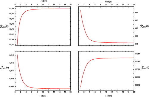
Table 3. Computation of the effective relaxation modulus and the effective creep compliance for the dermis. The input parameters are given in Tables 1, 2 and Figure 2.

Time (days)	${\widehat{\mathcal{R}}}_{1111}$ (Gpa)	${\widehat{\mathcal{R}}}_{1122}$ (Gpa)	${\widehat{\mathcal{R}}}_{2222}$ (Gpa)	${\widehat{\mathcal{R}}}_{3333}$ (Gpa)	${\widehat{\mathcal{R}}}_{1313}$ (Gpa)	${\widehat{\mathcal{R}}}_{1212}$ (Gpa)
0.8	135.0019	106.9072	112.8124	123.5786	8.3665	4.8150
2.9	134.9209	106.9500	112.6385	123.4420	8.2800	4.6759
5.1	134.9042	106.9588	112.6021	123.4137	8.2621	4.6441
7.2	134.9008	106.9606	112.5948	123.4080	8.2585	4.6377
9.3	134.8996	106.9612	112.5923	123.4060	8.2573	4.6357
11.5	134.8991	106.9615	112.5912	123.4052	8.2568	4.6348
13.6	134.8989	106.9616	112.5907	123.4048	8.2565	4.6343
15.7	134.8987	106.9617	112.5903	123.4045	8.2563	4.6340
17.9	134.8986	106.9617	112.5901	123.4043	8.2562	4.6338
20	134.8986	106.9618	112.5900	123.4042	8.2561	4.6337
time (days)	${\widehat{\mathcal{J}}}_{1111}$ (Gpa)	${\widehat{\mathcal{J}}}_{1122}$ (Gpa)	${\widehat{\mathcal{J}}}_{2222}$ (Gpa)	${\widehat{\mathcal{J}}}_{3333}$ (Gpa)	${\widehat{\mathcal{J}}}_{1313}$ (Gpa)	${\widehat{\mathcal{J}}}_{1212}$ (Gpa)
0.8	0.031562	−0.02154	0.06103	0.04534	0.031020	0.053881
2.9	0.031766	−0.02192	0.06215	0.04585	0.031324	0.055452
5.1	0.031806	−0.02201	0.06239	0.04594	0.031379	0.055813
7.2	0.031815	−0.02202	0.06243	0.04596	0.031391	0.055885
9.3	0.031817	−0.02203	0.06245	0.04597	0.031395	0.055908
11.5	0.031819	−0.02203	0.06246	0.04597	0.031396	0.055918
13.6	0.031819	−0.02203	0.06246	0.04597	0.031397	0.055923
15.7	0.03182	−0.02203	0.06246	0.04597	0.031398	0.055926
17.9	0.03182	−0.02203	0.06246	0.04597	0.031398	0.055928
20	0.03182	−0.02203	0.06246	0.04597	0.031398	0.05593

In Figure 3, we focus on the behavior of some chosen coefficients: ${\widehat{\mathcal{R}}}_{2233},{\widehat{\mathcal{R}}}_{2323},{\widehat{\mathcal{J}}}_{2233},{\widehat{\mathcal{J}}}_{2323}.$ As observed, the curves present an asymptotic behavior, which have a good agreement with the physical relaxation and creep response in viscoelastic materials for long times. Moreover, the monotony changes and the convexities for $\widehat{\mathcal{R}}$ and $\widehat{\mathcal{J}}$ in the same components, for instance, ${\widehat{\mathcal{R}}}_{2233}$ and ${\widehat{\mathcal{J}}}_{2233}$ are opposite. This behavior is a consequence of the Eq. (59)(59) $${\widehat{\mathcal{R}}}_{\mathit{ijmn}}(p){\widehat{\mathcal{J}}}_{\mathit{mnkl}}(p)=I_{\mathit{ijkl}},$$(59) and the fact that ${\widehat{\mathcal{R}}}_{\mathit{ijmn}}(p)$ and ${\widehat{\mathcal{J}}}_{\mathit{mnkl}}(p)$ are inverse tensors. Similar patterns have been remarked in other works (see Ref. 42, 43]).

6. Conclusions

A general methodology in the use of the three-scale Asymptotic Homogenization Method (AHM) is considered for modeling non-aging, quasi-periodic, hierarchical and linear viscoelastic composite materials. The present work takes into account the stratified functions in the homogenization procedure allowing the study with more general periodic structures. The analytical solution for the local problems and the expressions of the effective coefficients for hierarchical laminated composites with anisotropic components and perfect contact at the interfaces are derived. Also, the interconnection between the effective relaxation modulus and the effective creep compliance is performed. The approach is applied to study the overall viscoelastic behavior of the dermis. The results shown in Table 3 and Figure 3 could have a special interest in clinical applications, for instance, in the study of the epidural anesthesia procedure and in the development of haptic devices used in surgical operations. Its study is important in order to provide a location as accurate as possible for the insertion of the needle and the mechanical response of the skin (see Ref. [44]). The results can be used in the automation of the needle insertion procedure (see Ref. [45]).

The theoretical framework that we have developed here can be applied to large variety of hierarchical tissues which exhibit a viscoelastic mechanical response and are characterized by a complex, tortuous geometry, such as solid tumors, see, e.g. Netti et al. [46]; Penta and Ambrosi [47]; Ramírez-Torres et al. [48]. A further development also includes the generalization to a viscoplastic framework by considering remodeling aspects Ramírez-Torres et al. [31]. Although in the most general case numerical simulations cannot be avoided, application of our generalized framework would enable us to encode most of the geometrical complexity analytically, rather than enforce it directly in the setup of the computational grid, thus leading to a substantial reduction of the computational cost.

Also, the article is open to several improvements; for instance, with the framework established to layered materials, it is possible to work with more realistic geometries (e.g. fiber-reinforced composites) by using the stratified functions in the general form ${\rho }^{(\alpha )}:{\mathbb{R}}^3\to {\mathbb{R}}^3,$ with $\alpha =y,z$ (see Ref. [10]). It represents a novel point of view in order to make comparisons with framework entirely developed to fiber elastic [12] and viscoelastic [16, 42] reinforced composites. Besides, the results can be extended to the case of imperfect contact conditions by following the methodology in Guinovart-Sanjuán et al. [35] and considering viscoelastic interfaces (see e.g. Ref. [49]) for each structural level. Another natural step is to generalize the present work to aging viscoelastic solids, see e.g. Sanahuja [50]. This way, the model will be applicable to much larger variety of biophysical (diseased and healthy) scenarios of interest.

Acknowledgements

OLCG kindly thanks to Ecole Doctorale no. 353 de L’Université de Aix Marseille and L’équipe Matériaux & Structures du Laboratoire de Mécanique et d’Acoustique LMA - UMR 7031 AMU - CNRS - Centrale Marseille 4 impasse Nikola Tesla CS 40006 13453 Marseille Cedex 13, France. RRR thanks to Departamento de Matemáticas y Mecánica, IIMAS and PREI-DGAPA at UNAM, for its support to his research project and the Aix-Marseille Université. The authors are thankful to Ana Pérez Arteaga and Ramiro Chávez Tovar for technical assistance. ART kindly acknowledges the Dipartimento di Scienze Matematiche (DISMA) “G.L. Lagrange” of the Politecnico di Torino, “Dipartimento di Eccellenza 2018–2022”, Project code: E11G18000350001. RP is partially supported by EPSRC grant (EP/S030875/1). Also, FJS thanks funding from DGAPA, UNAM.

References

- I. Sevostianov and A. Giraud, Generalization of Maxwell homogenization scheme for elastic material containing inhomogeneities of diverse shape, Int. J. Eng. Sci., vol. 64, pp. 23–36, 2013. DOI: https://doi.org/10.1016/j.ijengsci.2012.12.004.
- Y. Davit, et al., Homogenization via formal multiscale asymptotics and volume averaging: How do the two techniques compare? Adv. Water Resource., vol. 62, pp. 178–206, 2013. DOI: https://doi.org/10.1016/j.advwatres.2013.09.006.
- D. Lukkassen and G. W. Milton, On hierarchical structures and reiterated homogenization. Proceedings of the International Conference in Honour of Jaak Peetre on his 65th birthday: Function Spaces, Interpolation Theory and Related Topics [Series: De Gruyter Proceedings in Mathematics], pp. 355–368, August 17–22, Lund, Sweden, 2000.
- R. Penta and A. Gerisch, The asymptotic homogenization elasticity tensor properties for composites with material discontinuities, Continuum Mech. Thermodyn., vol. 29, no. 1, pp. 187–206, 2017. DOI: https://doi.org/10.1007/s00161-016-x.
- A. Ramírez-Torres, S. D. Stefano, A. Grillo, R. Rodríguez-Ramos, J. Merodio, and J. Penta, Three scales asymptotic homogenization and its application to layered hierarchical hard tissues, Int. J. Solids Struct., vol. 130–131, pp. 190–198, 2018a. DOI: https://doi.org/10.1016/j.ijsolstr.2017.09.035.
- A. Ramírez-Torres, P. Penta, R. Rodríguez-Ramos, and A. Grillo, Homogenized out-of-plane shear response of three-scale fiberreinforced composites, Comput. Visual. Sci., vol. 20, no. 3–6, pp. 85–93, 2019a. DOI: https://doi.org/10.1007/s00791-018-0301-6.
- Z. Yang, Y. Sun, Y. Liu, T. Guan, and H. Dong, A three-scale asymptotic expansion for predicting viscoelastic properties of composites with multiple configuration, Eur. J. Mech. A. Solids., vol. 76, pp. 235–246, 2019b. DOI: https://doi.org/10.1016/j.euromechsol.2019.04.016.
- H. Dong, X. Zheng, J. Cui, Y. Nie, Z. Yang, and Z. Yang, High-order three-scale computational method for dynamic thermo-mechanical problems of composite structures with multiple spatial scales, Int. J. Solids Struct., vol. 169, pp. 95–121, 2019. DOI: https://doi.org/10.1016/j.ijsolstr.2019.04.017.
- D. Tsalis, G. Chatzigeorgiou, and N. Charalambakis, Homogenization of structures with generalized periodicity, Composites Part B. Eng., vol. 43, no. 6, pp. 2495–2512, 2012. DOI: https://doi.org/10.1016/j.compositesb.2012.01.054.
- D. Tsalis, T. Baxevanis, G. Chatzigeorgiou, and N. Charalambakis, Homogenization of elastoplastic composites with generalized periodicity in the microstructure, Int. J. Plasti., vol. 51, pp. 161–187, 2013. DOI: https://doi.org/10.1016/j.ijplas.2013.05.006.
- R. Penta, K. Raum, Q. Grimal, S. Schrof, and A. Gerisch, Can a continuous mineral foam explain the stiffening of aged bone tissue? A micromechanical approach to mineral fusion in musculoskeletal tissues, Bioinspir. Biomim., vol. 11, no. 3, pp. 035004, 2016. DOI: https://doi.org/10.1088/1748-3190/11/3/035004.
- A. Ramírez-Torres, et al., Effective properties of hierarchical fiber-reinforced composites via a three-scale asymptotic homogenization approach, Math. Mech. Solid., vol. 24, no. 11, pp. 3554–3574, 2019b. DOI: https://doi.org/10.1177/1081286519847687.
- G. Allaire and M. Briane, Multiscale convergence and reiterated homogenisation, Proc. R. Soc. Edin. Sec. A. Math., vol. 126, no. 2, pp. 297–342, 1996. DOI: https://doi.org/10.1017/S0308210500022757.
- A. Bensoussan, G. Papanicolau, and J.-L. Lions, Asymptotic Analysis for Periodic Structures, 1st ed., Vol. 5. Elsevier, North-Holland, 1978.
- D. Trucu, M. Chaplain, and A. Marciniak-Czochra, Three-scale convergence for processes in heterogeneous media, Applicable Anal., vol. 91, no. 7, pp. 1351–1373, 2012. DOI: https://doi.org/10.1080/00036811.2011.569498.
- Z. Yang, Y. Sun, J. Cui, and J. Ge, A three-scale asymptotic analysis for ageing linear viscoelastic problems of composites with multiple configurations, Appl. Mathe. Model., vol. 71, pp. 223–242, 2019a. DOI: https://doi.org/10.1016/j.apm.2019.02.021.
- O. L. Cruz-González, et al., An approach for modeling non-ageing linear viscoelastic composites with general periodicity, Composite Structures., vol. 223, pp. 110927, 2019. DOI: https://doi.org/10.1016/j.compstruct.2019.110927.
- Y.-M. Yi, S.-H. Park, and S.-K. Youn, Asymptotic homogenization of viscoelastic composites with periodic microstructures, Int. J. Solids Struct., vol. 35, no. 17, pp. 2039–2055, 1998. DOI: https://doi.org/10.1016/S0020-7683(97)00166-2.
- S. Liu, K.-Z. Chen, and X.-A. Feng, Prediction of viscoelastic property of layered materials, Int. J. Solids Struct., vol. 41, no. 13, pp. 3675–3688, 2004. DOI: https://doi.org/10.1016/j.ijsolstr.2004.01.015.
- A. B. Tran, J. Yvonnet, Q.-C. He, C. Toulemonde, and J. Sanahuja, A simple computational homogenization method for structures made of linear heterogeneous viscoelastic materials, Comput. Method. Appl. Mech. Eng., vol. 200, no. 45–46, pp. 2956–2970, 2011. DOI: https://doi.org/10.1016/j.cma.2011.06.012.
- V. R. Sherman, Y. Tang, S. Zhao, W. Yang, and M. A. Meyers, Structural characterization and viscoelastic constitutive modeling of skin, Acta Biomater., vol. 53, pp. 460–469, 2017. DOI: https://doi.org/10.1016/j.actbio.2017.02.011.
- A. N. Annaidh, K. Bruyère, M. Destrade, M. D. Gilchrist, and M. Otténio, Characterization of the anisotropic mechanical properties of excised human skin, J. Mech. Beh. Biomed. Materi., vol. 5, no. 1, pp. 139–148, 2012. DOI: https://doi.org/10.1016/j.jmbbm.2011.08.016.
- D. Malhotra, et al., Linear viscoelastic and microstructural properties of native male human skin and in vitro 3D reconstructed skin models, J. Mech. Behav. Biomed. Mater., vol. 90, pp. 644–654, 2019. DOI: https://doi.org/10.1016/j.jmbbm.2018.11.013.
- W. Yang, et al., On the tear resistance of skin, Nat. Commun., vol. 6, no. 6649, pp. 6, 2015. DOI: https://doi.org/10.1038/ncomms7649.
- R. Panchal, L. Horton, P. Poozesh, J. Baqersad, and M. Nasiriavanaki, Vibration analysis of healthy skin: toward a noninvasive skin diagnosis methodology, J. Biomed. Opt., vol. 24, no. 1, 2019. DOI: https://doi.org/10.1117/1.JBO.24.1.015001.
- I. Muha, A. Naegel, S. Sabine, A. Grillo, M. Heisig, and G. Wittum, Effective diffusivity in membranes with tetrakaidekahedral cells and implications for the permeability of human stratum corneum, J. Membr. Sci., vol. 368, no. 1-2, pp. 18–25, 2011. DOI: https://doi.org/10.1016/j.memsci.2010.10.020.
- J. M. Benítez and F. J. Montáns, The mechanical behavior of skin: Structures and models for the finite element analysis, Comput. Struct., vol. 190, pp. 75–107, 2017. DOI: https://doi.org/10.1016/j.compstruc.2017.05.003.
- Z. Hashin, Viscoelastic Behavior of Heterogeneous Media, J. Appl. Mech., vol. 32, no. 3, pp. 630–636, 1965. DOI: https://doi.org/10.1115/1.3627270.
- Q.-D. To, S.-T. Nguyen, G. Bonnet and M.-N. Vu, Overall viscoelastic properties of 2D and two-phase periodic composites constituted of elliptical and rectangular heterogeneities, Eur. J. Mech. A. Solids., vol. 64, pp. 186–201, 2017. DOI: https://doi.org/10.1016/j.euromechsol.2017.03.004.
- J. L. Auriault, C. Boutin, and C. Geindreau, Homogenization of Coupled Phenomena in Heterogenous Media, Wiley, New York, 2009.
- A. Ramírez-Torres, et al., An asymptotic homogenization approach to the microstructural evolution of heterogeneous media, Int. J. Non- Linear Mech., vol. 106, pp. 245–257, 2018b. DOI: https://doi.org/10.1016/j.ijnonlinmec.2018.06.012.
- R. M. Christensen, Theory of Viscoelasticity - 2nd Edition an Introduction, Academic Press, Cambridge, MA, 1982.
- S. Maghous and G. J. Creus, Periodic homogenization in thermoviscoelasticity: case of multilayered media with ageing, Int. J. Solids Struct., vol. 40, no. 4, pp. 851–870, 2003. DOI: https://doi.org/10.1016/S0020-7683(02)00549-8.
- E. Sanchez-Palencia, Non-Homogeneous Media and Vibration Theory. Lecture Notes in Physics. Berlin: Springer-Verlag, 1980.
- D. Guinovart-Sanjuán, et al., Analysis of effective elastic properties for shell with complex geometrical shapes, Composite Struct., vol. 203, pp. 278–285, 2018. DOI: https://doi.org/10.1016/j.compstruct.2018.07.036.
- H. Joodaki and M. B. Panzer, Skin mechanical properties and modeling: A review, Proc. Inst. Mech. Eng. H., vol. 232, no. 4, pp. 323–343, 2018. DOI: https://doi.org/10.1177/0954411918759801.
- F. Xu and T. Lu, Introduction to Skin Bio-Thermo Mechanics and Thermal Pain, Vol. 7. New York: Springer, 2011.
- A. McBride, S. Bargmann, D. Pond, and G. Limbert, Thermoelastic modelling of the skin at finite deformations, J. Therm. Biol., vol. 62, pp. 201–209, 2016. DOI: https://doi.org/10.1016/j.jtherbio.2016.06.017.
- Z. Hashin, Theory of fiber reinforced materials. NASA Contractor Report, Washington DC, USA, Rep. NASA CR-1974, 1972.
- K. J. Hollenbeck, Invlap. M: A Matlab function for numerical inversion of Laplace transforms by the Hoog algorithm. 1998. http://www.isva.dtu.dk/staff/karl/invlap.html.
- W. Srigutomo, Gaver-Stehfest algorithm for inverse Laplace transform, 2006. www.mathworks.com/matlabcentral/fileexchange/9987.
- M. A. Araújo-Cavalcante and S. P. Cavalcanti-Marques, Homogenization of periodic materials with viscoelastic phases using the generalized FVDAM theory, Comput. Mater. Sci., vol. 87, pp. 43–53, 2014. DOI: https://doi.org/10.1016/j.commatsci.2014.01.053.
- M. A. Araújo-Cavalcante and S. P. Cavalcanti-Marques, Microstructure effects in wavy-multilayers with viscoelastic phases, Eur. J. Mech. A. Solids., vol. 64, pp. 178–185, 2017. DOI: https://doi.org/10.1016/j.euromechsol.2017.03.003.
- D. Gao, Y. Lei, and B. Yao, Analysis of dynamic tissue deformation during needle insertion into soft tissue, IFAC Proc., vol. 46, no. 5, pp. 684–691, 2013.
- N. Abolhassani, R. Patel, and M. Moallem, Experimental study of robotic needle insertion in soft tissue, Int. Congr. Ser., vol. 1268, pp. 797–802, 2004. DOI: https://doi.org/10.1016/j.ics.2004.03.110.
- P. A. Netti, D. A. Berk, M. A. Swartz, A. J. Grodzinsky, and R. K. Jain, Role of extracellular matrix assembly in interstitial transport in solid tumors, Cancer Res., vol. 60, no. 9, pp. 2497–2503, 2000.
- R. Penta and D. Ambrosi, The role of the microvascular tortuosity in tumor transport phenomena, J. Theoret. Biol., vol. 364, pp. 80–97, 2015. DOI: https://doi.org/10.1016/j.jtbi.2014.08.007.
- A. Ramírez-Torres, et al., The role of malignant tissue on the thermal distribution of cancerous breast, J. Theoret. Biol., vol. 426, pp. 152–161, 2017. DOI: https://doi.org/10.1016/j.jtbi.2017.05.031.
- L. Daridon, C. Licht, S. Orankitjaroen, and S. Pagano, Periodic homogenization for Kelvin-Voigt viscoelastic media with a Kelvin-Voigt viscoelastic interphase, Eur. J. Mech. A. Solids., vol. 58, pp. 163–171, 2016. DOI: https://doi.org/10.1016/j.euromechsol.2015.12.007.
- J. Sanahuja, Effective behaviour of ageing linear viscoelastic composites: Homogenization approach, Int. J. Solids Struct., vol. 50, no. 19, pp. 2846–2856, 2013. DOI: https://doi.org/10.1016/j.ijsolstr.2013.04.023.