Stiffness and stress fluctuations in dental cement paste: a continuum micromechanics approach

Abstract

Calcite-reinforced hydrates provide the superior mechanical properties of Biodentine, a cementitious material used in dentistry. Herein, a self-consistent micromechanics model links two nanoindentation-probed, lognormally distributed microstiffness distributions of infinitely many hydrate phases, to the material’s macrostiffness, quantified from longitudinal and transverse ultrasonic wave transmission experiments. Thereby, the model provides values for the Poisson’s ratio of the hydrates and for a microcrack density reflecting grain boundary defects. Moreover, the model-predicted hydrate microstresses turn out as beta-distributed, while the overall stiffness can be equally well upscaled from only two, piecewise uniform, hydrate phases exhibiting median microstiffness values.

Highlights

• Grid nanoindentation provides lognormal distributions of hydrate stiffness

• They enter a microelastic model for dental cement paste

• This model considers grain boundary defects as isotropically-oriented closed cracks

• It provides micro-stress fluctuations resulting from hydrate stiffness distributions

• Median values of hydrate stiffness govern the overall paste stiffness

Keywords:

• Stiffness homogenization
• stiffness fluctuations
• stress fluctuations
• dental cement paste
• continuum micromechanics
• lognormal microelasticity model
• piecewise uniform microelasticity model

1. Introduction

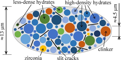
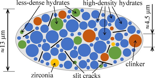
Biodentine is a cementitious material used in dentistry. The main hydraulic component is tricalcium silicate (“clinker”), making up 74 wt% of the dry binder powder [1, 2]. Calcite (16.5 wt%) acts as a filler and reinforcement [3]. Zirconium dioxide (“zirconia”, 5 wt%) provides X-ray opacity. The mixing liquid consists of water, a modified polycarboxylate polymer (= superplasticizer), and calcium chloride accelerating the setting reaction [1, 2]. The present paper refers to micromechanics modeling of the elastic stiffness of well-hardened Biodentine, based on results from a grid nanoindentation testing campaign [3].

Using results from grid nanoindentation as microscopic input for microelastic modeling of cement paste was introduced by Constantinides and Ulm [4]. They performed 200 indentation tests into the calcium-silicate-hydrate matrix. The 200 resulting values of indentation moduli were translated into moduli of elasticity, assuming a Poisson’s ratio of 0.24 [5]. The histogram of the moduli of elasticity showed two peaks. They were represented by the superposition of two Gaussian probability density functions. Their mean values were used as input for upscaling of the elastic stiffness of cement paste, delivering a homogenized modulus of elasticity amounting to $23.2\text{GPa}.$ As for validation, the speed of longitudinal ultrasonic waves passing through the tested material, its mass density, and its Poisson’s ratio (set equal to 0.24) were translated, based on the theory of elastic wave propagation through isotropic media, into the macroscopic modulus of elasticity: $22.8\text{GPa}$ [4]. This success motivated follow-up developments, see the discussion section, and it provides the motivation for the present contribution. Focused on Biodentine, it is aimed at linking microstructural stiffness distributions by means of a micromechanics model to the macroscopic effective (= homogenized) stiffness of the material.

As regards microscopic characterization of Biodentine, results from a grid nanoindentation testing campaign are taken from [3]. 5748 nanoindentation tests were performed with a Berkovich tip. Imposing maximum indentation forces of $1\text{mN}$ resulted in maximum indentation depths of on average $140\text{nm}.$ Only two experiments had to be excluded, because their maximum indentation depths were smaller than $45\text{nm}$ and, therefore, did not satisfy the requirement of being at least 2.5-times larger than the root-mean-squared average surface roughness [6, 7], which amounted to $18\text{nm}$ [3]. 5746 force-displacement diagrams were evaluated based on the Oliver-Pharr formulae for nanoindentation into infinite halfspaces [8]. The obtained histogram of the indentation modulus was represented by the superposition of three lognormal probability density functions, see Fig. 1. Lognormal distributions were used rather than Gaussians, because (i) indentation moduli are strictly positive quantities, and (ii) the large number of indentation experiments revealed skewed rather than symmetric stiffness distributions. The rightmost lognormal distribution in Fig. 1 refers to both clinker and zirconia, the central distribution to high-density calcite-reinforced hydrates (“HDCR hydrates”), and the leftmost to lower-density calcite-reinforced hydrates (“LDCR hydrates”), see [3] and Table 1. This reveals the existence of two types of hydrates reinforced by calcite particles of single-to-submicrometric size [9]. The two populations of hydrates are reminiscent of construction cement pastes in which inner and outer products [10], phenograin and groundmass [11], low-density and high-density C-S-H [12, 13], as well as class-A and class-B C-S-H [14] are distinguished.

Figure 1. Histogram of indentation modulus approximated by the superposition of three lognormal distributions; after [3].

Table 1. Results obtained from grid nanoindentation testing [3]: values of medians, modes, and volume fractions associated with the three lognormal distributions representing the histogram of indentation moduli in Fig. 1.

Lognormal distribution	Median [GPa]	Mode [GPa]	Volume fraction [–]
LDCR hydrates	45.1	24.5	0.1228
HDCR hydrates	62.6	60.2	0.7420
clinker and zirconia	92.2	89.0	0.1352
		sum:	1.0000

Evaluation of nanoindentation tests into the stiff clinker and zirconia grains, based on the Oliver-Pharr formulae mentioned above, led to smaller-than-expected indentation moduli, because the grains acted as a kind of larger indenters pressed into the softer surrounding hydrated material. This effect has been shown explicitly by image-supported grid nanoindentation, applied to two different types of cementitious materials [15, 16]. Hence, we resort to the well-known elastic properties of clinker and zirconia which are taken from the literature, see Table 2. The volume fractions of all four types of solid constituents are taken from [3].

Table 2. Input quantities of the solid material constituents: bulk moduli, k_i, shear moduli g_i, as well as lognormal parameters μ_i and σ_i which are consistent with median and mode values listed in Table 1; input values taken from [3, 17, 18].

Phase	Index	Stiffness properties		Volume fraction
zirconia	i = 1	$k_1=170.8$ GPa	$g_1=78.8$ GPa	$f_1=0.0182$
clinker	i = 2	$k_2=116.7$ GPa	$g_2=53.8$ GPa	$f_2=0.1170$
HDCR hydrates	i = 3	${\mu }_3=4.14$	${\sigma }_3=0.20$	$f_3=0.7420$
LDCR hydrates	i = 4	${\mu }_4=3.81$	${\sigma }_4=0.78$	$f_4=0.1228$

As regards macroscopic characterization of Biodentine, the speed of longitudinal ultrasonic waves and the mass density were reported in [3]. Herein, also the speed of transversal ultrasonic waves sent through well-hardened Biodentine is provided, see Appendix A. This allows for the complete characterization of the macroscopic isotropic stiffness of the material: (1) $$k_{\mathit{bio}}^{\hspace{0.17em}\mathit{\text{exp}}\hspace{0.17em}}=38.4\text{GPa},$$(1) (2) $$g_{\mathit{bio}}^{\hspace{0.17em}\mathit{\text{exp}}\hspace{0.17em}}=14.1\text{GPa},$$(2) where $k_{\mathit{bio}}^{\hspace{0.17em}\mathit{\text{exp}}\hspace{0.17em}}$ and $g_{\mathit{bio}}^{\hspace{0.17em}\mathit{\text{exp}}\hspace{0.17em}}$ denote the macroscopic bulk and shear moduli of Biodentine; for details see Appendix A.

The micromechanics model will also account for grain boundary defects. This is motivated as follows. Micromechanical stiffness bounds were computed for Biodentine, based on median stiffness values and volume fractions of the three lognormal distributions [3]. The lower bound for the stiffness tensor component C₁₁₁₁ turned out to be significantly larger than the value of C₁₁₁₁ derived from the ultrasonic longitudinal wave transmission experiments. This analysis indicated the existence of zero-volume microstructural defects such as imperfect grain boundaries.

The focus of the present contribution rests on the development of a micromechanics model which establishes a quantitative link between the microstructural stiffness properties (see Fig. 1 and Tables 1 and 2) and the macroscopic effective stiffness of Biodentine, see Eqs. (1)(1) $$k_{\mathit{bio}}^{\hspace{0.17em}\mathit{\text{exp}}\hspace{0.17em}}=38.4\text{GPa},$$(1) and (2)(2) $$g_{\mathit{bio}}^{\hspace{0.17em}\mathit{\text{exp}}\hspace{0.17em}}=14.1\text{GPa},$$(2) , with two remarkable features:

• Grain boundary defects will be accounted for in a self-consistent homogenization approach. They will be modeled by means of closed circular cracks which are isotropically oriented in space. Budiansky and O’Connell’s dimensionless crack density parameter [19, 20] will be quantified from linking the micromechanical model to both nanoindentation and ultrasonic test results.

• The lognormal distributions of the indentation modulus of the two populations of calcite-reinforced hydrates will serve as input for the micromechanics model, rather than just one representative stiffness per population. Poisson’s ratio of the two populations of calcite-reinforced hydrates will be quantified from linking the micromechanical model to both nanoindentation and ultrasonic test results.

The described micromechanics model will be used to illustrate quantitatively how macroscopic uniform loading imposed on a representative volume of Biodentine results in microscopic stress and strain distributions inside the two populations of hydrates.

The lognormal microelasticity model will also allow for assessing the potential and the limitations of piecewise uniform microelasticity models. The latter are based on just one representative stiffness per population of calcite-reinforced hydrates. This is particularly interesting in case of skewed probability density functions (Fig. 1) in which the mode (= most frequent value), the median (= 50%-quantile), and the mean value are different, while they are all the same in case of Gaussians.

The present paper is structured as follows: Section 2 presents the lognormal microelasticity model for Biodentine, accounting for the microstiffness distributions of the two populations of hydrates by means of two times infinitely many material phases. Section 3 is dedicated to stress and strain fluctuations within the hydrates of Biodentine, quantified by means of probability density functions of volumetric and deviatoric strain and stress concentration tensor components of the two populations of hydrates. Section 4 deals with piecewise uniform microelasticity models in which one “equivalent” uniform stiffness is assigned to each one of the two populations of hydrates. Section 5 contains a discussion. Section 6 closes the paper with conclusions drawn from results of the presented study.

2. Lognormal microelasticity model for Biodentine

2.1. Fundamentals of stiffness homogenization

Stiffness homogenization refers to a boundary value problem of the linear theory of elasticity. It is defined on a representative volume element (RVE) with volume V of the microheterogeneous material of interest.

The field equations refer to all positions $\underset{¯}{x}$ inside V. The linear geometric equations define the linearized strain tensor $\mathit{\epsilon }$ as the symmetric part of the displacement gradient. Denoting the displacement vector as $\underset{¯}{u},$ they read as $\mathit{\epsilon }(\underset{¯}{x})=\frac{1}{2}[\nabla \underset{¯}{u}(\underset{¯}{x})+\nabla {\underset{¯}{u}}^T\mathrm{}(\underset{¯}{x})].$ The linear constitutive relations refer to linear elastic material behavior. Denoting Cauchy’s stress tensor as $\mathit{\sigma }$ and the elasticity tensor as $\mathbb{C},$ they read as $\mathit{\sigma }(\underset{¯}{x})=\mathbb{C}(\underset{¯}{x}):\mathit{\epsilon }(\underset{¯}{x}).$ The stresses must fulfill the equilibrium conditions, reading as $\text{div}\mathit{\sigma }(\underset{¯}{x})=0.$

The boundary conditions refer to all positions $\underset{¯}{x}$ at the surface $\partial V$ of the representative volume. Herein, uniform strain boundary conditions are used [21]. Denoting the imposed macroscopic strain state as E, they read as (3) $$\underset{¯}{u}(\underset{¯}{x})=\mathbf{E}·\underset{¯}{x}.$$(3) Homogenization of the elastic stiffness is facilitated through the introduction of quasi-homogeneous constituents of the microheterogeneous material. Denoted as material phases, they occupy specific subvolumes V_i of the representative volume V. Their volume fractions read as $f_i=V_i/V,$ with $i=1,2,\dots ,N,$ where N denotes the number of material phases. In addition, material phases are characterized by specific elastic stiffness tensors ${\mathbb{C}}_i.$ Average phase strains and stresses are introduced: (4) $${\mathit{\epsilon }}_i=\frac{1}{V_i}\underset{V_i}{\overset{}{\int }}\mathit{\epsilon }(\underset{¯}{x}) \mathrm{d}V,\mathrm{\hspace{1em}}\mathrm{\hspace{1em}}i=1,2,\dots ,N,$$(4) (5) $${\mathit{\sigma }}_i=\frac{1}{V_i}\underset{V_i}{\overset{}{\int }}\mathit{\sigma }(\underset{¯}{x}) \mathrm{d}V,\mathrm{\hspace{1em}}\mathrm{\hspace{1em}}i=1,2,\dots ,N.$$(5) Boundary conditions (3(3) $$\underset{¯}{u}(\underset{¯}{x})=\mathbf{E}·\underset{¯}{x}.$$(3) ) and the principle of virtual power [22] imply the existence of the following strain and stress average rules: (6) $$\mathbf{E}=\sum _{i=1}^N{f}_i{\mathit{\epsilon }}_i,$$(6) (7) $$\mathbf{\Sigma }=\sum _{i=1}^N{f}_i{\mathit{\sigma }}_i,$$(7) where $\mathbf{\Sigma }$ denotes the macroscopic stress state. Because the stiffness is uniform inside the phase volumes V_i, the phase-specific version of the elasticity law reads as: (8) $${\mathit{\sigma }}_i={\mathbb{C}}_i:{\mathit{\epsilon }}_i,\mathrm{\hspace{1em}}\mathrm{\hspace{1em}}i=1,2,\dots ,N.$$(8) Macro-to-micro and micro-to-macro scale transitions are made possible by so-called strain concentration tensors ${\mathbb{A}}_i.$ They establish links between the macrostrain and the average phase strains [23–26]: (9) $${\mathit{\epsilon }}_i={\mathbb{A}}_i:\mathbf{E},\mathrm{\hspace{1em}}\mathrm{\hspace{1em}}i=1,2,\dots ,N.$$(9) Strain concentration tensors also allow for bottom-up stiffness homogenization, as will be explained next. Inserting ${\mathit{\epsilon }}_i$ according to Eq. (9)(9) $${\mathit{\epsilon }}_i={\mathbb{A}}_i:\mathbf{E},\mathrm{\hspace{1em}}\mathrm{\hspace{1em}}i=1,2,\dots ,N.$$(9) into Eq. (8)(8) $${\mathit{\sigma }}_i={\mathbb{C}}_i:{\mathit{\epsilon }}_i,\mathrm{\hspace{1em}}\mathrm{\hspace{1em}}i=1,2,\dots ,N.$$(8) , and the resulting expression for ${\mathit{\sigma }}_i$ into Eq. (7)(7) $$\mathbf{\Sigma }=\sum _{i=1}^N{f}_i{\mathit{\sigma }}_i,$$(7) yields a relation between the macrostress $\mathbf{\Sigma }$ and the macrostrain E. Comparing it with the macroscopic version of the elasticity law, (10) $$\Sigma ={\mathbb{C}}_{\mathit{hom}}:\mathit{E},$$(10) delivers the following expression for the homogenized stiffness tensor [23, 26] (11) $${\mathbb{C}}_{\mathit{hom}}=\sum _{i=1}^N{f}_i{\mathbb{C}}_i:{\mathbb{A}}_i.$$(11) Stress concentration tensors ${\mathbb{B}}_i$ establish links between the macrostress and the average phase stresses: (12) $${\mathit{\sigma }}_i={\mathbb{B}}_i:\mathbf{\Sigma },\mathrm{\hspace{1em}}\mathrm{\hspace{1em}}i=1,2,\dots ,N.$$(12) The stress concentration tensors are related to the strain concentration tensors, as will be shown next. The macroscopic elasticity law (10(10) $$\Sigma ={\mathbb{C}}_{\mathit{hom}}:\mathit{E},$$(10) ) is solved for the macrostrain: $\mathbf{E}={({\mathbb{C}}_{\mathit{hom}})}^{-1}:\mathbf{\Sigma }.$ Inserting it into Eq. (9)(9) $${\mathit{\epsilon }}_i={\mathbb{A}}_i:\mathbf{E},\mathrm{\hspace{1em}}\mathrm{\hspace{1em}}i=1,2,\dots ,N.$$(9) and the resulting expression for ${\mathit{\epsilon }}_i$ into Eq. (8)(8) $${\mathit{\sigma }}_i={\mathbb{C}}_i:{\mathit{\epsilon }}_i,\mathrm{\hspace{1em}}\mathrm{\hspace{1em}}i=1,2,\dots ,N.$$(8) yields a relation between the microstresses ${\mathit{\sigma }}_i$ and the macrostress $\mathbf{\Sigma }.$ Comparing this relation with Eq. (12)(12) $${\mathit{\sigma }}_i={\mathbb{B}}_i:\mathbf{\Sigma },\mathrm{\hspace{1em}}\mathrm{\hspace{1em}}i=1,2,\dots ,N.$$(12) yields (13) $${\mathbb{B}}_i={\mathbb{C}}_i:{\mathbb{A}}_i:{({\mathbb{C}}_{\mathit{hom}})}^{-1},\mathrm{\hspace{1em}}\mathrm{\hspace{1em}}i=1,2,\dots ,N.$$(13) Eqs. (9)(9) $${\mathit{\epsilon }}_i={\mathbb{A}}_i:\mathbf{E},\mathrm{\hspace{1em}}\mathrm{\hspace{1em}}i=1,2,\dots ,N.$$(9) , (11)(11) $${\mathbb{C}}_{\mathit{hom}}=\sum _{i=1}^N{f}_i{\mathbb{C}}_i:{\mathbb{A}}_i.$$(11) , and (13)(13) $${\mathbb{B}}_i={\mathbb{C}}_i:{\mathbb{A}}_i:{({\mathbb{C}}_{\mathit{hom}})}^{-1},\mathrm{\hspace{1em}}\mathrm{\hspace{1em}}i=1,2,\dots ,N.$$(13) underline that strain concentration tensors enable scale transitions in continuum micromechanics. These strain concentration tensors are estimated from Eshelby/Laws-type matrix-inclusion problems [27, 28]. This will be explained in more detail in the context of the following development of a lognormal microelasticity model for Biodentine.

2.2. Tensorial formulation of lognormal microelasticity model for Biodentine

Continuum micromechanics models account for key features of microheterogeneous materials: the stiffness constants of the material phases, their volume fractions, their characteristic phase shapes, and the specific type of interaction between the phases. Biodentine consists of five types of constituents: zirconia (index i = 1), clinker (i = 2), HDCR hydrates (i = 3), LDCR hydrates (i = 4), and grain boundary defects modeled as closed microcracks (i = 5). The microstructure of Biodentine is represented as a highly disordered (“polycrystalline”) arrangement of material constituents which exhibit direct phase-to-phase interaction, see Fig. 2.

Figure 2. Micromechanical representation of Biodentine (“material organogram”): the two-dimensional sketch shows qualitative properties of a three-dimensional representative volume element of the lognormal microelasticity model which accounts for stiffness distributions of two populations of hydrates.

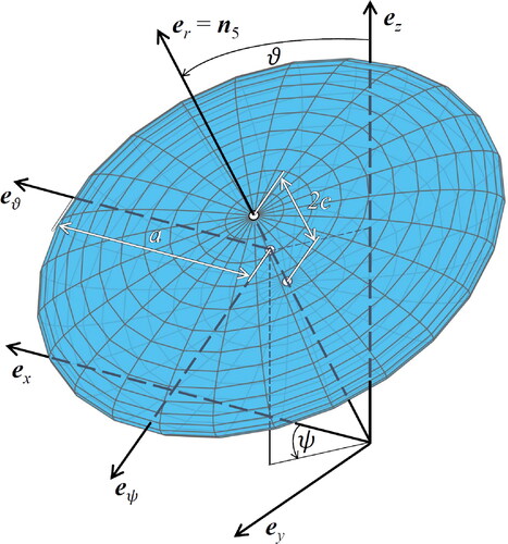
As regards phase shapes, all four types of solid constituents are represented as spherical phases. The microcracks are introduced as thin oblate spheroids.¹ Because they are isotropically oriented in space, they will be represented as a population of infinitely many material phases [29, 30].

Zirconia and clinker are isotropic, with constant (invariant) stiffness tensors reading as (14) $${\mathbb{C}}_i=3k_i{\mathbb{I}}^{\mathit{vol}}+2g_i{\mathbb{I}}^{\mathit{dev}},\mathrm{\hspace{1em}}\mathrm{\hspace{1em}}i=1,2,$$(14) where k_i and g_i denote the bulk and shear moduli, see Table 2. ${\mathbb{I}}^{\mathit{vol}}$ and ${\mathbb{I}}^{\mathit{dev}}$ stand for the volumetric and deviatoric parts of the symmetric fourth-order identity tensor $\mathbb{I}.$ Their components read as $I_{\mathit{ijkl}}=\left({\delta }_{ik}{\delta }_{jl}+{\delta }_{il}{\delta }_{jk}\right)\mathrm{}/2,$ $I_{\mathit{ijkl}}^{\mathit{vol}}=\left({\delta }_{ij}{\delta }_{kl}\right)\mathrm{}/3,$ and $I_{\mathit{ijkl}}^{\mathit{dev}}=I_{\mathit{ijkl}}-I_{\mathit{ijkl}}^{\mathit{vol}},$ where δ_ij is the Kronecker delta which is equal to 1 for i = j, and equal to 0 otherwise. ${\mathbb{I}}^{\mathit{vol}}$ and ${\mathbb{I}}^{\mathit{dev}}$ satisfy the following relations: (15) $${\mathbb{I}}^{\mathit{vol}}:{\mathbb{I}}^{\mathit{vol}}={\mathbb{I}}^{\mathit{vol}},$$(15) (16) $${\mathbb{I}}^{\mathit{dev}}:{\mathbb{I}}^{\mathit{dev}}={\mathbb{I}}^{\mathit{dev}},$$(16) (17) $${\mathbb{I}}^{\mathit{vol}}:{\mathbb{I}}^{\mathit{dev}}=0,$$(17) (18) $${\mathbb{I}}^{\mathit{dev}}:{\mathbb{I}}^{\mathit{vol}}=0.$$(18) The two populations of hydrates exhibit lognormal stiffness distributions, see Table 1. The probability distribution functions of their indentation moduli M read as: (19) $${\phi }_i(M)=\frac{1}{M{\sigma }_i\sqrt{2\pi }}\hspace{0.17em}\text{exp}\hspace{0.17em}\mathrm{}(\mathrm{}-\frac{1}{2}{\left[\frac{\hspace{0.17em}\text{ln}\hspace{0.17em}(M)-{\mu }_i}{{\sigma }_i}\right]}^2),\hspace{1em}i=3,4.$$(19) By definition, the area under the graphs of the probability density functions (19(19) $${\phi }_i(M)=\frac{1}{M{\sigma }_i\sqrt{2\pi }}\hspace{0.17em}\text{exp}\hspace{0.17em}\mathrm{}(\mathrm{}-\frac{1}{2}{\left[\frac{\hspace{0.17em}\text{ln}\hspace{0.17em}(M)-{\mu }_i}{{\sigma }_i}\right]}^2),\hspace{1em}i=3,4.$$(19) ) is equal to 1: (20) $$\underset{0}{\overset{\infty }{\int }}{\phi }_i(M) \mathrm{d}M=1,\mathrm{\hspace{1em}}\mathrm{\hspace{1em}}i=3,4.$$(20) The continuous stiffness distributions of both populations of hydrates are accounted for in the continuum micromechanics model by representing each one of the two populations of hydrates as infinitely many material phases; the latter exhibiting infinitesimally small volume fractions. The material phases making up the RVE are complemented by two additional phases with finite volume fractions, representing zirconia and clinker, and by infinitely many crack phases.

The self-consistent scheme is well suited for homogenization of materials with highly disordered “polycrystalline” microstructure [26]. One Eshelby-type matrix-inclusion problem is formulated for each and every material phase, irrespective of whether they exhibit finite or infinitesimal volume fractions, see Fig. 3. The inclusion has the stiffness, the shape, and the orientation of the material phase it is representing. The stiffness of the infinitely large matrix is equal to that of the homogenized composite (here: Biodentine, index bio). This specific property of the self-consistent scheme expresses that the material phases are directly interacting with all constituents of the microheterogeneous material [26]. Remotely, the matrices of all of the infinitely many Eshelby problems are subjected to the same auxiliary strain state ${\mathbf{E}}_{\infty }.$ The strains in the inclusions are spatially uniform and read as [27] (21) $${\mathit{\epsilon }}_i={[\mathbb{I}+{\mathbb{P}}_{\mathit{sph}}:({\mathbb{C}}_i-{\mathbb{C}}_{\mathit{bio}})]}^{-1}:{\mathbf{E}}_{\infty },\hspace{1em}i=1,2,$$(21) (22) $${\mathit{\epsilon }}_i(M)={[\mathbb{I}+{\mathbb{P}}_{\mathit{sph}}:({\mathbb{C}}_i(M)-{\mathbb{C}}_{\mathit{bio}})]}^{-1}:{\mathbf{E}}_{\infty },\hspace{1em}i=3,4,\hspace{1em}M\in {ℝ}^{0,+},$$(22) (23) $${\mathit{\epsilon }}_5(\psi ,\vartheta )={[\mathbb{I}+{\mathbb{P}}_{\mathit{obl}}(\psi ,\vartheta ):({\mathbb{C}}_5-{\mathbb{C}}_{\mathit{bio}})]}^{-1}:{\mathbf{E}}_{\infty },\psi \in [0,2\pi ],\hspace{1em}\vartheta \in [0,\pi ].$$(23) where ${ℝ}^{0,+}$ denotes all positive real numbers including zero. ${\mathbb{P}}_{\mathit{sph}}$ and ${\mathbb{P}}_{\mathit{obl}}$ denote the Hill tensors of spherical and oblate phases, respectively. ${\mathbb{P}}_{\mathit{obl}}$ is a function of Euler angles ψ and ϑ, see [31] and Fig. 4. The stiffness tensors of hydrates, see ${\mathbb{C}}_i(M)$ in Eq. (22)(22) $${\mathit{\epsilon }}_i(M)={[\mathbb{I}+{\mathbb{P}}_{\mathit{sph}}:({\mathbb{C}}_i(M)-{\mathbb{C}}_{\mathit{bio}})]}^{-1}:{\mathbf{E}}_{\infty },\hspace{1em}i=3,4,\hspace{1em}M\in {ℝ}^{0,+},$$(22) , are parametrized using the indentation modulus M, see Subsection 2.6 for details. The stiffness tensor of the microcracks, see ${\mathbb{C}}_5$ in Eq. (23)(23) $${\mathit{\epsilon }}_5(\psi ,\vartheta )={[\mathbb{I}+{\mathbb{P}}_{\mathit{obl}}(\psi ,\vartheta ):({\mathbb{C}}_5-{\mathbb{C}}_{\mathit{bio}})]}^{-1}:{\mathbf{E}}_{\infty },\psi \in [0,2\pi ],\hspace{1em}\vartheta \in [0,\pi ].$$(23) , is purely volumetric, see Subsection 2.3 for more details.

Figure 3. Eshelby-type matrix inclusion problems: (a) spherical inclusion, and (b) oblate spheroid, both embedded in an infinite matrix with isotropic stiffness ${\mathrm{C}}_{\mathit{bio}}$, subjected remotely to auxiliary uniform strains ${\mathbf{E}}_{\infty }.$

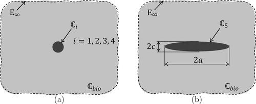
Figure 4. Thin oblate spheroid oriented in ψ,ϑ-direction.

It is a key step to establish relations between the auxiliary Eshelby problems described above, and the actual RVE of Biodentine [26]. To this end, the Eshelby-problem-related inclusion strains according to Eqs. (21)–(23) are used as estimates of the average strains of the corresponding material phases inside the real representative volume of Biodentine, see Eq. (4)(4) $${\mathit{\epsilon }}_i=\frac{1}{V_i}\underset{V_i}{\overset{}{\int }}\mathit{\epsilon }(\underset{¯}{x}) \mathrm{d}V,\mathrm{\hspace{1em}}\mathrm{\hspace{1em}}i=1,2,\dots ,N,$$(4) . The latter satisfy the strain average rule, see Eq. (6)(6) $$\mathbf{E}=\sum _{i=1}^N{f}_i{\mathit{\epsilon }}_i,$$(6) . When inserting Eqs. (21)–(23) into Eq. (6)(6) $$\mathbf{E}=\sum _{i=1}^N{f}_i{\mathit{\epsilon }}_i,$$(6) , the sum extending over two populations of infinitely many hydrate phases turns into the sum of two integrals, and the sum extending over infinitely many crack phases turns into a double-integral: (24) $$\begin{array}{c}\mathbf{E}=\sum _{j=1}^2{f}_j{[\mathbb{I}+{\mathbb{P}}_{\mathit{sph}}:({\mathbb{C}}_j-{\mathbb{C}}_{\mathit{bio}})]}^{-1}:{\mathbf{E}}_{\infty }\\ +\sum _{j=3}^4{f}_j\underset{0}{\overset{\infty }{\int }}{\phi }_j(M){[\mathbb{I}+{\mathbb{P}}_{\mathit{sph}}:({\mathbb{C}}_j(M)-{\mathbb{C}}_{\mathit{bio}})]}^{-1} \mathrm{d}M:{\mathbf{E}}_{\infty }\\ +f_5\mathrm{ }\underset{0}{\overset{\pi }{\int }}\underset{0}{\overset{2\pi }{\int }}{[\mathbb{I}+{\mathbb{P}}_{\mathit{obl}}(\psi ,\vartheta ):({\mathbb{C}}_5-{\mathbb{C}}_{\mathit{bio}})]}^{-1} \frac{\hspace{0.17em}\text{sin}\hspace{0.17em}\vartheta }{4\pi } d\psi d\vartheta :{\mathbf{E}}_{\infty }.\end{array}$$(24) Eq. (24)(24) $$\begin{array}{c}\mathbf{E}=\sum _{j=1}^2{f}_j{[\mathbb{I}+{\mathbb{P}}_{\mathit{sph}}:({\mathbb{C}}_j-{\mathbb{C}}_{\mathit{bio}})]}^{-1}:{\mathbf{E}}_{\infty }\\ +\sum _{j=3}^4{f}_j\underset{0}{\overset{\infty }{\int }}{\phi }_j(M){[\mathbb{I}+{\mathbb{P}}_{\mathit{sph}}:({\mathbb{C}}_j(M)-{\mathbb{C}}_{\mathit{bio}})]}^{-1} \mathrm{d}M:{\mathbf{E}}_{\infty }\\ +f_5\mathrm{ }\underset{0}{\overset{\pi }{\int }}\underset{0}{\overset{2\pi }{\int }}{[\mathbb{I}+{\mathbb{P}}_{\mathit{obl}}(\psi ,\vartheta ):({\mathbb{C}}_5-{\mathbb{C}}_{\mathit{bio}})]}^{-1} \frac{\hspace{0.17em}\text{sin}\hspace{0.17em}\vartheta }{4\pi } d\psi d\vartheta :{\mathbf{E}}_{\infty }.\end{array}$$(24) establishes a link between the loading of the representative volume of Biodentine (= the macrostrain E) and the loading of the auxiliary Eshelby problems (= the auxiliary strain ${\mathbf{E}}_{\infty }$). Solving Eq. (24)(24) $$\begin{array}{c}\mathbf{E}=\sum _{j=1}^2{f}_j{[\mathbb{I}+{\mathbb{P}}_{\mathit{sph}}:({\mathbb{C}}_j-{\mathbb{C}}_{\mathit{bio}})]}^{-1}:{\mathbf{E}}_{\infty }\\ +\sum _{j=3}^4{f}_j\underset{0}{\overset{\infty }{\int }}{\phi }_j(M){[\mathbb{I}+{\mathbb{P}}_{\mathit{sph}}:({\mathbb{C}}_j(M)-{\mathbb{C}}_{\mathit{bio}})]}^{-1} \mathrm{d}M:{\mathbf{E}}_{\infty }\\ +f_5\mathrm{ }\underset{0}{\overset{\pi }{\int }}\underset{0}{\overset{2\pi }{\int }}{[\mathbb{I}+{\mathbb{P}}_{\mathit{obl}}(\psi ,\vartheta ):({\mathbb{C}}_5-{\mathbb{C}}_{\mathit{bio}})]}^{-1} \frac{\hspace{0.17em}\text{sin}\hspace{0.17em}\vartheta }{4\pi } d\psi d\vartheta :{\mathbf{E}}_{\infty }.\end{array}$$(24) for ${\mathbf{E}}_{\infty }$ yields (25) $$\begin{array}{c}{\mathbf{E}}_{\infty }=\{\sum _{j=1}^2{f}_j{[\mathbb{I}+{\mathbb{P}}_{\mathit{sph}}:({\mathbb{C}}_j-{\mathbb{C}}_{\mathit{bio}})]}^{-1}\\ +\sum _{j=3}^4{f}_j\underset{0}{\overset{\infty }{\int }}{\phi }_j(M){[\mathbb{I}+{\mathbb{P}}_{\mathit{sph}}:({\mathbb{C}}_j(M)-{\mathbb{C}}_{\mathit{bio}})]}^{-1} \mathrm{d}M\\ +f_5\mathrm{ }\underset{0}{\overset{\pi }{\int }}\underset{0}{\overset{2\pi }{\int }}{[\mathbb{I}+{\mathbb{P}}_{\mathit{obl}}(\psi ,\vartheta ):({\mathbb{C}}_5-{\mathbb{C}}_{\mathit{bio}})]}^{-1} \frac{\hspace{0.17em}\text{sin}\hspace{0.17em}\vartheta }{4\pi } d\psi d\vartheta {\}}^{-1}:\mathbf{E}.\end{array}$$(25) Inserting Eq. (25)(25) $$\begin{array}{c}{\mathbf{E}}_{\infty }=\{\sum _{j=1}^2{f}_j{[\mathbb{I}+{\mathbb{P}}_{\mathit{sph}}:({\mathbb{C}}_j-{\mathbb{C}}_{\mathit{bio}})]}^{-1}\\ +\sum _{j=3}^4{f}_j\underset{0}{\overset{\infty }{\int }}{\phi }_j(M){[\mathbb{I}+{\mathbb{P}}_{\mathit{sph}}:({\mathbb{C}}_j(M)-{\mathbb{C}}_{\mathit{bio}})]}^{-1} \mathrm{d}M\\ +f_5\mathrm{ }\underset{0}{\overset{\pi }{\int }}\underset{0}{\overset{2\pi }{\int }}{[\mathbb{I}+{\mathbb{P}}_{\mathit{obl}}(\psi ,\vartheta ):({\mathbb{C}}_5-{\mathbb{C}}_{\mathit{bio}})]}^{-1} \frac{\hspace{0.17em}\text{sin}\hspace{0.17em}\vartheta }{4\pi } d\psi d\vartheta {\}}^{-1}:\mathbf{E}.\end{array}$$(25) into Eqs. (21)–(23) and comparing the results with Eq. (9)(9) $${\mathit{\epsilon }}_i={\mathbb{A}}_i:\mathbf{E},\mathrm{\hspace{1em}}\mathrm{\hspace{1em}}i=1,2,\dots ,N.$$(9) yields the following estimates for the strain concentration tensors of clinker and zirconia (26) $$\begin{array}{l}{\mathbb{A}}_i={[\mathbb{I}+{\mathbb{P}}_{sph}:({\mathbb{C}}_i-{\mathbb{C}}_{bio})]}^{-1}\\ :\{{\displaystyle \sum _{j=1}^2{f}_j}{[\mathbb{I}+{\mathbb{P}}_{sph}:({\mathbb{C}}_j-{\mathbb{C}}_{bio})]}^{-1}\\ +{\displaystyle \sum _{j=3}^4{f}_j}{\displaystyle \underset{0}{\overset{\infty }{\int }}{\phi }_j(M){[\mathbb{I}+{\mathbb{P}}_{sph}:({\mathbb{C}}_j(M)-{\mathbb{C}}_{bio})]}^{-1} \text{d}M}\\ +f_5{\displaystyle \underset{0}{\overset{\pi }{\int }}{\displaystyle \underset{0}{\overset{2\pi }{\int }}{[\mathbb{I}+{\mathbb{P}}_{obl}(\psi ,\vartheta ):({\mathbb{C}}_5-{\mathbb{C}}_{bio})]}^{-1} \frac{\sin \vartheta }{4\pi } d\psi d\vartheta {\}}^{-1},}}\\ i=1,2,\end{array}$$(26) of the hydrate phases (27) $$\begin{array}{c}{\mathbb{A}}_i(M)={[\mathbb{I}+{\mathbb{P}}_{\mathit{sph}}:({\mathbb{C}}_i(M)-{\mathbb{C}}_{\mathit{bio}})]}^{-1}\\ :\{\sum _{j=1}^2{f}_j{[\mathbb{I}+{\mathbb{P}}_{\mathit{sph}}:({\mathbb{C}}_j-{\mathbb{C}}_{\mathit{bio}})]}^{-1}\\ +\sum _{j=3}^4{f}_j\underset{0}{\overset{\infty }{\int }}{\phi }_j(N){[\mathbb{I}+{\mathbb{P}}_{\mathit{sph}}:({\mathbb{C}}_j(N)-{\mathbb{C}}_{\mathit{bio}})]}^{-1} dN\\ +f_5\underset{0}{\overset{\pi }{\int }}\underset{0}{\overset{2\pi }{\int }}{[\mathbb{I}+{\mathbb{P}}_{\mathit{obl}}(\psi ,\vartheta ):({\mathbb{C}}_5-{\mathbb{C}}_{\mathit{bio}})]}^{-1} \frac{\hspace{0.17em}\text{sin}\hspace{0.17em}\vartheta }{4\pi } d\psi d\vartheta {\}}^{-1},\\ \hspace{1em}i=3,4,\hspace{1em}M\in {ℝ}^{0,+},\end{array}$$(27) and of the microcracks (28) $$\begin{array}{c}{\mathbb{A}}_5(\psi ,\vartheta )={[\mathbb{I}+{\mathbb{P}}_{\mathit{obl}}(\psi ,\vartheta ):({\mathbb{C}}_5-{\mathbb{C}}_{\mathit{bio}})]}^{-1}\\ :\{\sum _{j=1}^2{f}_j{[\mathbb{I}+{\mathbb{P}}_{\mathit{sph}}:({\mathbb{C}}_j-{\mathbb{C}}_{\mathit{bio}})]}^{-1}\\ +\sum _{j=3}^4{f}_j\underset{0}{\overset{\infty }{\int }}{\phi }_j(M){[\mathbb{I}+{\mathbb{P}}_{\mathit{sph}}:({\mathbb{C}}_j(M)-{\mathbb{C}}_{\mathit{bio}})]}^{-1} \mathrm{d}M\\ +f_5\underset{0}{\overset{\pi }{\int }}\underset{0}{\overset{2\pi }{\int }}{[\mathbb{I}+{\mathbb{P}}_{\mathit{obl}}(\chi ,\vartheta ):({\mathbb{C}}_5-{\mathbb{C}}_{\mathit{bio}})]}^{-1} \frac{\hspace{0.17em}\text{sin}\hspace{0.17em}\vartheta }{4\pi } d\chi d\vartheta {\}}^{-1},\\ \hspace{1em}\psi \in [0,2\pi ],\hspace{1em}\vartheta \in [0,\pi ].\end{array}$$(28) The homogenized stiffness of Biodentine follows from inserting Eqs. (26)–(28) into Eq. (11)(11) $${\mathbb{C}}_{\mathit{hom}}=\sum _{i=1}^N{f}_i{\mathbb{C}}_i:{\mathbb{A}}_i.$$(11) as (29) $$\begin{array}{c}{\mathbb{C}}_{\mathit{bio}}=\{\sum _{i=1}^2{f}_i{\mathbb{C}}_i:{[\mathbb{I}+{\mathbb{P}}_{\mathit{sph}}:({\mathbb{C}}_i-{\mathbb{C}}_{\mathit{bio}})]}^{-1}\\ +\sum _{i=3}^4{f}_i\underset{0}{\overset{\infty }{\int }}{\phi }_i(M){\mathbb{C}}_i(M):{[\mathbb{I}+{\mathbb{P}}_{\mathit{sph}}:({\mathbb{C}}_i(M)-{\mathbb{C}}_{\mathit{bio}})]}^{-1} \mathrm{d}M\\ +f_5{\mathbb{C}}_5:\underset{0}{\overset{\pi }{\int }}\underset{0}{\overset{2\pi }{\int }}{[\mathbb{I}+{\mathbb{P}}_{\mathit{obl}}(\psi ,\vartheta ):({\mathbb{C}}_5-{\mathbb{C}}_{\mathit{bio}})]}^{-1} \frac{\hspace{0.17em}\text{sin}\hspace{0.17em}\vartheta }{4\pi } d\psi d\vartheta \}\\ :\{\sum _{j=1}^2{f}_j{[\mathbb{I}+{\mathbb{P}}_{\mathit{sph}}:({\mathbb{C}}_j-{\mathbb{C}}_{\mathit{bio}})]}^{-1}\\ +\sum _{j=3}^4{f}_j\underset{0}{\overset{\infty }{\int }}{\phi }_j(M){[\mathbb{I}+{\mathbb{P}}_{\mathit{sph}}:({\mathbb{C}}_j(M)-{\mathbb{C}}_{\mathit{bio}})]}^{-1} \mathrm{d}M\\ +f_5\mathrm{ }\underset{0}{\overset{\pi }{\int }}\underset{0}{\overset{2\pi }{\int }}{[\mathbb{I}+{\mathbb{P}}_{\mathit{obl}}(\psi ,\vartheta ):({\mathbb{C}}_5-{\mathbb{C}}_{\mathit{bio}})]}^{-1} \frac{\hspace{0.17em}\text{sin}\hspace{0.17em}\vartheta }{4\pi } d\psi d\vartheta {\}}^{-1}.\end{array}$$(29)

2.3. Transition to flat circular slit cracks

Microcracks are invisible in micrographs of Biodentine [3]. This indicates that the cracks are closed. Their volume fraction is zero. Thus, the effect of closed cracks on the overall material behavior cannot be traced back to their volume fraction. Instead, the crack density parameter of Budiansky and O’Connell [19] is introduced, see also [20, 32]. To this end, cracks are first represented as thin oblate spheroids, with a as the larger half-diameter, c as the smaller half-diameter, and very small aspect ratio $X=c/a\ll 1.$ The volume of one such spheroid reads as: $4\pi a^{2}c/3.$ Thus, the volume fraction of thin spheroidal cracks inside a representative volume of Biodentine amounts to (30) $$f_5=\frac{N_{cr}}{V_{\mathit{bio}}}\frac{4\pi a^{2}c}{3},$$(30) where N_cr denotes to number of cracks within one representative volume V_bio of Biodentine. Introducing the dimensionless crack density parameter as $\omega =N_{cr}{a}^3/V_{\mathit{bio}},$ Eq. (30)(30) $$f_5=\frac{N_{cr}}{V_{\mathit{bio}}}\frac{4\pi a^{2}c}{3},$$(30) can be re-written as (31) $$f_5=\frac{4\pi \omega }{3}X.$$(31) The Hill tensor ${\mathbb{P}}_{\mathit{obl}}$ can be expressed as the Eshelby tensor ${\mathbb{S}}_{\mathit{obl}}$ double-contracted with the inverse of the stiffness tensor of Biodentine [29]: (32) $${\mathbb{P}}_{\mathit{obl}}={\mathbb{S}}_{\mathit{obl}}:{({\mathbb{C}}_{\mathit{bio}})}^{-1},$$(32) where ${\mathbb{S}}_{\mathit{obl}}$ is a function of the aspect ratio X, see Appendix C . The stiffness tensor ${\mathbb{C}}_5$ is purely volumetric, because the shear stiffness of closed cracks vanishes [29] (33) $${\mathbb{C}}_5=3k_5{\mathbb{I}}^{\mathit{vol}}.$$(33) Because of the following limit case $X\to 0,$ the actual value of k₅ does not matter, as long as it is positive and finite: $0<k_5<\infty ,$ see [29]. Inserting Eqs. (31)–(33) into the expression in the last line of Eq. (29)(29) $$\begin{array}{c}{\mathbb{C}}_{\mathit{bio}}=\{\sum _{i=1}^2{f}_i{\mathbb{C}}_i:{[\mathbb{I}+{\mathbb{P}}_{\mathit{sph}}:({\mathbb{C}}_i-{\mathbb{C}}_{\mathit{bio}})]}^{-1}\\ +\sum _{i=3}^4{f}_i\underset{0}{\overset{\infty }{\int }}{\phi }_i(M){\mathbb{C}}_i(M):{[\mathbb{I}+{\mathbb{P}}_{\mathit{sph}}:({\mathbb{C}}_i(M)-{\mathbb{C}}_{\mathit{bio}})]}^{-1} \mathrm{d}M\\ +f_5{\mathbb{C}}_5:\underset{0}{\overset{\pi }{\int }}\underset{0}{\overset{2\pi }{\int }}{[\mathbb{I}+{\mathbb{P}}_{\mathit{obl}}(\psi ,\vartheta ):({\mathbb{C}}_5-{\mathbb{C}}_{\mathit{bio}})]}^{-1} \frac{\hspace{0.17em}\text{sin}\hspace{0.17em}\vartheta }{4\pi } d\psi d\vartheta \}\\ :\{\sum _{j=1}^2{f}_j{[\mathbb{I}+{\mathbb{P}}_{\mathit{sph}}:({\mathbb{C}}_j-{\mathbb{C}}_{\mathit{bio}})]}^{-1}\\ +\sum _{j=3}^4{f}_j\underset{0}{\overset{\infty }{\int }}{\phi }_j(M){[\mathbb{I}+{\mathbb{P}}_{\mathit{sph}}:({\mathbb{C}}_j(M)-{\mathbb{C}}_{\mathit{bio}})]}^{-1} \mathrm{d}M\\ +f_5\mathrm{ }\underset{0}{\overset{\pi }{\int }}\underset{0}{\overset{2\pi }{\int }}{[\mathbb{I}+{\mathbb{P}}_{\mathit{obl}}(\psi ,\vartheta ):({\mathbb{C}}_5-{\mathbb{C}}_{\mathit{bio}})]}^{-1} \frac{\hspace{0.17em}\text{sin}\hspace{0.17em}\vartheta }{4\pi } d\psi d\vartheta {\}}^{-1}.\end{array}$$(29) , and subjecting the result to the limit $X\to 0,$ which expresses that the volume occupied by closed cracks is negligibly small, yields [29] (34) $$\begin{array}{c}\underset{X\to 0}{\lim }{f}_5(X)\underset{0}{\overset{\pi }{\int }}\underset{0}{\overset{2\pi }{\int }}{[\mathbb{I}+{\mathbb{P}}_{\mathit{obl}}(X,\psi ,\vartheta ):({\mathbb{C}}_5-{\mathbb{C}}_{\mathit{bio}})]}^{-1} \frac{\hspace{0.17em}\text{sin}\hspace{0.17em}\vartheta }{4\pi } d\psi d\vartheta \\ \mathrm{\hspace{1em}}\mathrm{\hspace{1em}}=\frac{4\pi \omega }{3}{T}_{\mathit{dev}}{\mathbb{I}}^{\mathit{dev}},\end{array}$$(34) with (35) $$T_{\mathit{dev}}=\frac{8(3k_{\mathit{bio}}+4g_{\mathit{bio}})}{15\pi (3k_{\mathit{bio}}+2g_{\mathit{bio}})}.$$(35) The third line in Eq. (29)(29) $$\begin{array}{c}{\mathbb{C}}_{\mathit{bio}}=\{\sum _{i=1}^2{f}_i{\mathbb{C}}_i:{[\mathbb{I}+{\mathbb{P}}_{\mathit{sph}}:({\mathbb{C}}_i-{\mathbb{C}}_{\mathit{bio}})]}^{-1}\\ +\sum _{i=3}^4{f}_i\underset{0}{\overset{\infty }{\int }}{\phi }_i(M){\mathbb{C}}_i(M):{[\mathbb{I}+{\mathbb{P}}_{\mathit{sph}}:({\mathbb{C}}_i(M)-{\mathbb{C}}_{\mathit{bio}})]}^{-1} \mathrm{d}M\\ +f_5{\mathbb{C}}_5:\underset{0}{\overset{\pi }{\int }}\underset{0}{\overset{2\pi }{\int }}{[\mathbb{I}+{\mathbb{P}}_{\mathit{obl}}(\psi ,\vartheta ):({\mathbb{C}}_5-{\mathbb{C}}_{\mathit{bio}})]}^{-1} \frac{\hspace{0.17em}\text{sin}\hspace{0.17em}\vartheta }{4\pi } d\psi d\vartheta \}\\ :\{\sum _{j=1}^2{f}_j{[\mathbb{I}+{\mathbb{P}}_{\mathit{sph}}:({\mathbb{C}}_j-{\mathbb{C}}_{\mathit{bio}})]}^{-1}\\ +\sum _{j=3}^4{f}_j\underset{0}{\overset{\infty }{\int }}{\phi }_j(M){[\mathbb{I}+{\mathbb{P}}_{\mathit{sph}}:({\mathbb{C}}_j(M)-{\mathbb{C}}_{\mathit{bio}})]}^{-1} \mathrm{d}M\\ +f_5\mathrm{ }\underset{0}{\overset{\pi }{\int }}\underset{0}{\overset{2\pi }{\int }}{[\mathbb{I}+{\mathbb{P}}_{\mathit{obl}}(\psi ,\vartheta ):({\mathbb{C}}_5-{\mathbb{C}}_{\mathit{bio}})]}^{-1} \frac{\hspace{0.17em}\text{sin}\hspace{0.17em}\vartheta }{4\pi } d\psi d\vartheta {\}}^{-1}.\end{array}$$(29) vanishes, because it is equal to the volumetric stiffness tensor ${\mathbb{C}}_5,$ see Eq. (33)(33) $${\mathbb{C}}_5=3k_5{\mathbb{I}}^{\mathit{vol}}.$$(33) , double-contracted with the expression on the left-hand-side of Eq. (34)(34) $$\begin{array}{c}\underset{X\to 0}{\lim }{f}_5(X)\underset{0}{\overset{\pi }{\int }}\underset{0}{\overset{2\pi }{\int }}{[\mathbb{I}+{\mathbb{P}}_{\mathit{obl}}(X,\psi ,\vartheta ):({\mathbb{C}}_5-{\mathbb{C}}_{\mathit{bio}})]}^{-1} \frac{\hspace{0.17em}\text{sin}\hspace{0.17em}\vartheta }{4\pi } d\psi d\vartheta \\ \mathrm{\hspace{1em}}\mathrm{\hspace{1em}}=\frac{4\pi \omega }{3}{T}_{\mathit{dev}}{\mathbb{I}}^{\mathit{dev}},\end{array}$$(34) , which is deviatoric, see also Eq. (17)(17) $${\mathbb{I}}^{\mathit{vol}}:{\mathbb{I}}^{\mathit{dev}}=0,$$(17) . Thus Eq. (29)(29) $$\begin{array}{c}{\mathbb{C}}_{\mathit{bio}}=\{\sum _{i=1}^2{f}_i{\mathbb{C}}_i:{[\mathbb{I}+{\mathbb{P}}_{\mathit{sph}}:({\mathbb{C}}_i-{\mathbb{C}}_{\mathit{bio}})]}^{-1}\\ +\sum _{i=3}^4{f}_i\underset{0}{\overset{\infty }{\int }}{\phi }_i(M){\mathbb{C}}_i(M):{[\mathbb{I}+{\mathbb{P}}_{\mathit{sph}}:({\mathbb{C}}_i(M)-{\mathbb{C}}_{\mathit{bio}})]}^{-1} \mathrm{d}M\\ +f_5{\mathbb{C}}_5:\underset{0}{\overset{\pi }{\int }}\underset{0}{\overset{2\pi }{\int }}{[\mathbb{I}+{\mathbb{P}}_{\mathit{obl}}(\psi ,\vartheta ):({\mathbb{C}}_5-{\mathbb{C}}_{\mathit{bio}})]}^{-1} \frac{\hspace{0.17em}\text{sin}\hspace{0.17em}\vartheta }{4\pi } d\psi d\vartheta \}\\ :\{\sum _{j=1}^2{f}_j{[\mathbb{I}+{\mathbb{P}}_{\mathit{sph}}:({\mathbb{C}}_j-{\mathbb{C}}_{\mathit{bio}})]}^{-1}\\ +\sum _{j=3}^4{f}_j\underset{0}{\overset{\infty }{\int }}{\phi }_j(M){[\mathbb{I}+{\mathbb{P}}_{\mathit{sph}}:({\mathbb{C}}_j(M)-{\mathbb{C}}_{\mathit{bio}})]}^{-1} \mathrm{d}M\\ +f_5\mathrm{ }\underset{0}{\overset{\pi }{\int }}\underset{0}{\overset{2\pi }{\int }}{[\mathbb{I}+{\mathbb{P}}_{\mathit{obl}}(\psi ,\vartheta ):({\mathbb{C}}_5-{\mathbb{C}}_{\mathit{bio}})]}^{-1} \frac{\hspace{0.17em}\text{sin}\hspace{0.17em}\vartheta }{4\pi } d\psi d\vartheta {\}}^{-1}.\end{array}$$(29) reads for closed cracks with crack density parameter ω: (36) $$\begin{array}{c}{\mathbb{C}}_{\mathit{bio}}=\{\sum _{i=1}^2{f}_i{\mathbb{C}}_i:{[\mathbb{I}+{\mathbb{P}}_{\mathit{sph}}:({\mathbb{C}}_i-{\mathbb{C}}_{\mathit{bio}})]}^{-1}\\ +\sum _{i=3}^4{f}_i\underset{0}{\overset{\infty }{\int }}{\phi }_i(M){\mathbb{C}}_i(M):{[\mathbb{I}+{\mathbb{P}}_{\mathit{sph}}:({\mathbb{C}}_i(M)-{\mathbb{C}}_{\mathit{bio}})]}^{-1} \mathrm{d}M\}\\ :\{\sum _{j=1}^2{f}_j{[\mathbb{I}+{\mathbb{P}}_{\mathit{sph}}:({\mathbb{C}}_j-{\mathbb{C}}_{\mathit{bio}})]}^{-1}\\ +\sum _{j=3}^4{f}_j\underset{0}{\overset{\infty }{\int }}{\phi }_j(M){[\mathbb{I}+{\mathbb{P}}_{\mathit{sph}}:({\mathbb{C}}_j(M)-{\mathbb{C}}_{\mathit{bio}})]}^{-1} \mathrm{d}M\\ +\frac{4\pi \omega }{3}{T}_{\mathit{dev}}{\mathbb{I}}^{\mathit{dev}}{\}}^{-1}.\end{array}$$(36)

2.4. Scalar expressions for the homogenized bulk and shear moduli

The Hill tensor ${\mathbb{P}}_{\mathit{sph}}$ can be expressed as the Eshelby tensor ${\mathbb{S}}_{\mathit{sph}}$ double-contracted with the inverse of the stiffness tensor of Biodentine [29]: (37) $${\mathbb{P}}_{\mathit{sph}}={\mathbb{S}}_{\mathit{sph}}:{({\mathbb{C}}_{\mathit{bio}})}^{-1}.$$(37) Because ${\mathbb{S}}_{\mathit{sph}}$ is isotropic, it can be expressed as (38) $${\mathbb{S}}_{\mathit{sph}}=S_{\mathit{vol}}{\mathbb{I}}^{\mathit{vol}}+S_{\mathit{dev}}{\mathbb{I}}^{\mathit{dev}},$$(38) with (39) $$S_{\mathit{vol}}=\frac{3k_{\mathit{bio}}}{3k_{\mathit{bio}}+4g_{\mathit{bio}}},$$(39) (40) $$S_{\mathit{dev}}=\frac{6(k_{\mathit{bio}}+2g_{\mathit{bio}})}{5(3k_{\mathit{bio}}+4g_{\mathit{bio}})}.$$(40) All tensors in Eqs. (36)(36) $$\begin{array}{c}{\mathbb{C}}_{\mathit{bio}}=\{\sum _{i=1}^2{f}_i{\mathbb{C}}_i:{[\mathbb{I}+{\mathbb{P}}_{\mathit{sph}}:({\mathbb{C}}_i-{\mathbb{C}}_{\mathit{bio}})]}^{-1}\\ +\sum _{i=3}^4{f}_i\underset{0}{\overset{\infty }{\int }}{\phi }_i(M){\mathbb{C}}_i(M):{[\mathbb{I}+{\mathbb{P}}_{\mathit{sph}}:({\mathbb{C}}_i(M)-{\mathbb{C}}_{\mathit{bio}})]}^{-1} \mathrm{d}M\}\\ :\{\sum _{j=1}^2{f}_j{[\mathbb{I}+{\mathbb{P}}_{\mathit{sph}}:({\mathbb{C}}_j-{\mathbb{C}}_{\mathit{bio}})]}^{-1}\\ +\sum _{j=3}^4{f}_j\underset{0}{\overset{\infty }{\int }}{\phi }_j(M){[\mathbb{I}+{\mathbb{P}}_{\mathit{sph}}:({\mathbb{C}}_j(M)-{\mathbb{C}}_{\mathit{bio}})]}^{-1} \mathrm{d}M\\ +\frac{4\pi \omega }{3}{T}_{\mathit{dev}}{\mathbb{I}}^{\mathit{dev}}{\}}^{-1}.\end{array}$$(36) and (37)(37) $${\mathbb{P}}_{\mathit{sph}}={\mathbb{S}}_{\mathit{sph}}:{({\mathbb{C}}_{\mathit{bio}})}^{-1}.$$(37) are isotropic. They can be subdivided into volumetric and deviatoric parts. Consideration of Eqs. (15)–(18) together with Eqs. (14)(14) $${\mathbb{C}}_i=3k_i{\mathbb{I}}^{\mathit{vol}}+2g_i{\mathbb{I}}^{\mathit{dev}},\mathrm{\hspace{1em}}\mathrm{\hspace{1em}}i=1,2,$$(14) , (37)(37) $${\mathbb{P}}_{\mathit{sph}}={\mathbb{S}}_{\mathit{sph}}:{({\mathbb{C}}_{\mathit{bio}})}^{-1}.$$(37) , and (40)(40) $$S_{\mathit{dev}}=\frac{6(k_{\mathit{bio}}+2g_{\mathit{bio}})}{5(3k_{\mathit{bio}}+4g_{\mathit{bio}})}.$$(40) in Eq. (36)(36) $$\begin{array}{c}{\mathbb{C}}_{\mathit{bio}}=\{\sum _{i=1}^2{f}_i{\mathbb{C}}_i:{[\mathbb{I}+{\mathbb{P}}_{\mathit{sph}}:({\mathbb{C}}_i-{\mathbb{C}}_{\mathit{bio}})]}^{-1}\\ +\sum _{i=3}^4{f}_i\underset{0}{\overset{\infty }{\int }}{\phi }_i(M){\mathbb{C}}_i(M):{[\mathbb{I}+{\mathbb{P}}_{\mathit{sph}}:({\mathbb{C}}_i(M)-{\mathbb{C}}_{\mathit{bio}})]}^{-1} \mathrm{d}M\}\\ :\{\sum _{j=1}^2{f}_j{[\mathbb{I}+{\mathbb{P}}_{\mathit{sph}}:({\mathbb{C}}_j-{\mathbb{C}}_{\mathit{bio}})]}^{-1}\\ +\sum _{j=3}^4{f}_j\underset{0}{\overset{\infty }{\int }}{\phi }_j(M){[\mathbb{I}+{\mathbb{P}}_{\mathit{sph}}:({\mathbb{C}}_j(M)-{\mathbb{C}}_{\mathit{bio}})]}^{-1} \mathrm{d}M\\ +\frac{4\pi \omega }{3}{T}_{\mathit{dev}}{\mathbb{I}}^{\mathit{dev}}{\}}^{-1}.\end{array}$$(36) yields (41) $$\begin{array}{c}{k}_{\mathit{bio}}=\{\sum _{i=1}^2\frac{f_i{k}_i}{1+\frac{S_{\mathit{vol}}(k_i-k_{\mathit{bio}})}{k_{\mathit{bio}}}}+\sum _{i=3}^4{f}_i\underset{0}{\overset{\infty }{\int }}\frac{{\phi }_i(M)k_i(M)}{1+\frac{S_{\mathit{vol}}(k_i(M)-k_{\mathit{bio}})}{k_{\mathit{bio}}}} \mathrm{d}M\}\\ \times {\{\sum _{i=1}^2\frac{f_i}{1+\frac{S_{\mathit{vol}}(k_i-k_{\mathit{bio}})}{k_{\mathit{bio}}}}+\sum _{i=3}^4{f}_i\mathrm{ }\underset{0}{\overset{\infty }{\int }}\frac{{\phi }_i(M)}{1+\frac{S_{\mathit{vol}}(k_i(M)-k_{\mathit{bio}})}{k_{\mathit{bio}}}} \mathrm{d}M\}}^{-1},\end{array}$$(41) (42) $$\begin{array}{c}{g}_{\mathit{bio}}=\{\sum _{i=1}^2\frac{f_i{g}_i}{1+\frac{S_{\mathit{dev}}(g_i-g_{\mathit{bio}})}{g_{\mathit{bio}}}}+\sum _{i=3}^4{f}_i\underset{0}{\overset{\infty }{\int }}\frac{{\phi }_i(M)g_i(M)}{1+\frac{S_{\mathit{dev}}(g_i(M)-g_{\mathit{bio}})}{g_{\mathit{bio}}}} \mathrm{d}M\}\\ \times \{\sum _{i=1}^2\frac{f_i}{1+\frac{S_{\mathit{dev}}(g_i-g_{\mathit{bio}})}{g_{\mathit{bio}}}}+\sum _{i=3}^4{f}_i\underset{0}{\overset{\infty }{\int }}\frac{{\phi }_i(M)}{1+\frac{S_{\mathit{dev}}(g_i(M)-g_{\mathit{bio}})}{g_{\mathit{bio}}}} \mathrm{d}M\\ \hspace{1em}+\frac{4\pi \omega }{3}{T}_{\mathit{dev}}{\}}^{-1}.\end{array}$$(42) The scalar Eqs. (41)(41) $$\begin{array}{c}{k}_{\mathit{bio}}=\{\sum _{i=1}^2\frac{f_i{k}_i}{1+\frac{S_{\mathit{vol}}(k_i-k_{\mathit{bio}})}{k_{\mathit{bio}}}}+\sum _{i=3}^4{f}_i\underset{0}{\overset{\infty }{\int }}\frac{{\phi }_i(M)k_i(M)}{1+\frac{S_{\mathit{vol}}(k_i(M)-k_{\mathit{bio}})}{k_{\mathit{bio}}}} \mathrm{d}M\}\\ \times {\{\sum _{i=1}^2\frac{f_i}{1+\frac{S_{\mathit{vol}}(k_i-k_{\mathit{bio}})}{k_{\mathit{bio}}}}+\sum _{i=3}^4{f}_i\mathrm{ }\underset{0}{\overset{\infty }{\int }}\frac{{\phi }_i(M)}{1+\frac{S_{\mathit{vol}}(k_i(M)-k_{\mathit{bio}})}{k_{\mathit{bio}}}} \mathrm{d}M\}}^{-1},\end{array}$$(41) and (42)(42) $$\begin{array}{c}{g}_{\mathit{bio}}=\{\sum _{i=1}^2\frac{f_i{g}_i}{1+\frac{S_{\mathit{dev}}(g_i-g_{\mathit{bio}})}{g_{\mathit{bio}}}}+\sum _{i=3}^4{f}_i\underset{0}{\overset{\infty }{\int }}\frac{{\phi }_i(M)g_i(M)}{1+\frac{S_{\mathit{dev}}(g_i(M)-g_{\mathit{bio}})}{g_{\mathit{bio}}}} \mathrm{d}M\}\\ \times \{\sum _{i=1}^2\frac{f_i}{1+\frac{S_{\mathit{dev}}(g_i-g_{\mathit{bio}})}{g_{\mathit{bio}}}}+\sum _{i=3}^4{f}_i\underset{0}{\overset{\infty }{\int }}\frac{{\phi }_i(M)}{1+\frac{S_{\mathit{dev}}(g_i(M)-g_{\mathit{bio}})}{g_{\mathit{bio}}}} \mathrm{d}M\\ \hspace{1em}+\frac{4\pi \omega }{3}{T}_{\mathit{dev}}{\}}^{-1}.\end{array}$$(42) allow for an iterative determination of the homogenized bulk and shear moduli of Biodentine.

2.5. Scalar expressions for volumetric and deviatoric strain and stress tensor components

The strain concentration tensors of the spherical solid phases are also isotropic (43) $${\mathbb{A}}_i=A_{\mathit{vol},i}{\mathbb{I}}^{\mathit{vol}}+A_{\mathit{dev},i}{\mathbb{I}}^{\mathit{dev}}.$$(43) The volumetric and deviatoric components of the strain concentrations tensors of zirconia (i = 1) and clinker (i = 2) follow from Eq. (26)(26) $$\begin{array}{l}{\mathbb{A}}_i={[\mathbb{I}+{\mathbb{P}}_{sph}:({\mathbb{C}}_i-{\mathbb{C}}_{bio})]}^{-1}\\ :\{{\displaystyle \sum _{j=1}^2{f}_j}{[\mathbb{I}+{\mathbb{P}}_{sph}:({\mathbb{C}}_j-{\mathbb{C}}_{bio})]}^{-1}\\ +{\displaystyle \sum _{j=3}^4{f}_j}{\displaystyle \underset{0}{\overset{\infty }{\int }}{\phi }_j(M){[\mathbb{I}+{\mathbb{P}}_{sph}:({\mathbb{C}}_j(M)-{\mathbb{C}}_{bio})]}^{-1} \text{d}M}\\ +f_5{\displaystyle \underset{0}{\overset{\pi }{\int }}{\displaystyle \underset{0}{\overset{2\pi }{\int }}{[\mathbb{I}+{\mathbb{P}}_{obl}(\psi ,\vartheta ):({\mathbb{C}}_5-{\mathbb{C}}_{bio})]}^{-1} \frac{\sin \vartheta }{4\pi } d\psi d\vartheta {\}}^{-1},}}\\ i=1,2,\end{array}$$(26) as (44) $$\begin{array}{c}{A}_{\mathit{vol},i}=\frac{1}{1+\frac{S_{\mathit{vol}}(k_i-k_{\mathit{bio}})}{k_{\mathit{bio}}}}\{\sum _{i=1}^2\frac{f_i}{1+\frac{S_{\mathit{vol}}(k_i-k_{\mathit{bio}})}{k_{\mathit{bio}}}}\\ +\sum _{i=3}^4{f}_i\mathrm{ }\underset{0}{\overset{\infty }{\int }}\frac{{\phi }_i(M)}{1+\frac{S_{\mathit{vol}}(k_i(M)-k_{\mathit{bio}})}{k_{\mathit{bio}}}} \mathrm{d}M{\}}^{-1},\end{array}$$(44) (45) $$\begin{array}{c}{A}_{\mathit{dev},i}=\frac{1}{1+\frac{S_{\mathit{dev}}(g_i-g_{\mathit{bio}})}{g_{\mathit{bio}}}}\{\sum _{i=1}^2\frac{f_i}{1+\frac{S_{\mathit{dev}}(g_i-g_{\mathit{bio}})}{g_{\mathit{bio}}}}\\ +\sum _{i=3}^4{f}_i\mathrm{ }\underset{0}{\overset{\infty }{\int }}\frac{{\phi }_i(M)}{1+\frac{S_{\mathit{dev}}(g_i(M)-g_{\mathit{bio}})}{g_{\mathit{bio}}}} \mathrm{d}M+\frac{4\pi \omega }{3}{T}_{\mathit{dev}}{\}}^{-1}.\end{array}$$(45) The volumetric and deviatoric components of the strain concentrations tensors of HDCR (i = 3) and LDCR (i = 4) hydrates follow from Eq. (27)(27) $$\begin{array}{c}{\mathbb{A}}_i(M)={[\mathbb{I}+{\mathbb{P}}_{\mathit{sph}}:({\mathbb{C}}_i(M)-{\mathbb{C}}_{\mathit{bio}})]}^{-1}\\ :\{\sum _{j=1}^2{f}_j{[\mathbb{I}+{\mathbb{P}}_{\mathit{sph}}:({\mathbb{C}}_j-{\mathbb{C}}_{\mathit{bio}})]}^{-1}\\ +\sum _{j=3}^4{f}_j\underset{0}{\overset{\infty }{\int }}{\phi }_j(N){[\mathbb{I}+{\mathbb{P}}_{\mathit{sph}}:({\mathbb{C}}_j(N)-{\mathbb{C}}_{\mathit{bio}})]}^{-1} dN\\ +f_5\underset{0}{\overset{\pi }{\int }}\underset{0}{\overset{2\pi }{\int }}{[\mathbb{I}+{\mathbb{P}}_{\mathit{obl}}(\psi ,\vartheta ):({\mathbb{C}}_5-{\mathbb{C}}_{\mathit{bio}})]}^{-1} \frac{\hspace{0.17em}\text{sin}\hspace{0.17em}\vartheta }{4\pi } d\psi d\vartheta {\}}^{-1},\\ \hspace{1em}i=3,4,\hspace{1em}M\in {ℝ}^{0,+},\end{array}$$(27) as (46) $$\begin{array}{c}{A}_{\mathit{vol},i}(M)=\frac{1}{1+\frac{S_{\mathit{vol}}(k_i(M)-k_{\mathit{bio}})}{k_{\mathit{bio}}}}\{\sum _{i=1}^2\frac{f_i}{1+\frac{S_{\mathit{vol}}(k_i-k_{\mathit{bio}})}{k_{\mathit{bio}}}}\\ +\sum _{i=3}^4{f}_i\mathrm{ }\underset{0}{\overset{\infty }{\int }}\frac{{\phi }_i(M)}{1+\frac{S_{\mathit{vol}}(k_i(M)-k_{\mathit{bio}})}{k_{\mathit{bio}}}} \mathrm{d}M{\}}^{-1},\end{array}$$(46) (47) $$\begin{array}{c}{A}_{\mathit{dev},i}(M)=\frac{1}{1+\frac{S_{\mathit{dev}}(g_i(M)-g_{\mathit{bio}})}{g_{\mathit{bio}}}}\{\sum _{i=1}^2\frac{f_i}{1+\frac{S_{\mathit{dev}}(g_i-g_{\mathit{bio}})}{g_{\mathit{bio}}}}\\ +\sum _{i=3}^4{f}_i\underset{0}{\overset{\infty }{\int }}\mathrm{ }\frac{{\phi }_i(M)}{1+\frac{S_{\mathit{dev}}(g_i(M)-g_{\mathit{bio}})}{g_{\mathit{bio}}}} \mathrm{d}M+\frac{4\pi \omega }{3}{T}_{\mathit{dev}}{\}}^{-1},\end{array}$$(47) where $M\in {ℝ}^{0,+}.$ Strain concentration tensors of the closed cracks will be discussed in Subsection 3.4.

The stress concentration tensors of the spherical solid phases are also isotropic (48) $${\mathbb{B}}_i=B_{\mathit{vol},i}{\mathbb{I}}^{\mathit{vol}}+B_{\mathit{dev},i}{\mathbb{I}}^{\mathit{dev}}.$$(48) Accounting for the isotropy of the tensors in Eq. (13)(13) $${\mathbb{B}}_i={\mathbb{C}}_i:{\mathbb{A}}_i:{({\mathbb{C}}_{\mathit{hom}})}^{-1},\mathrm{\hspace{1em}}\mathrm{\hspace{1em}}i=1,2,\dots ,N.$$(13) delivers (49) $$B_{\mathit{vol},i}=\frac{k_i}{k_{\mathit{bio}}}{A}_{\mathit{vol},i},$$(49) (50) $$B_{\mathit{dev},i}=\frac{g_i}{g_{\mathit{bio}}}{A}_{\mathit{dev},i},$$(50) with k_i and g_i being the bulk and shear moduli of i-th phase, k_bio and g_bio are bulk and shear moduli of the homogenized composite Biodentine. The volumetric and deviatoric components of the stress concentrations tensors of zirconia (i = 1) and clinker (i = 2) follow from insertion of Eqs. (44)(44) $$\begin{array}{c}{A}_{\mathit{vol},i}=\frac{1}{1+\frac{S_{\mathit{vol}}(k_i-k_{\mathit{bio}})}{k_{\mathit{bio}}}}\{\sum _{i=1}^2\frac{f_i}{1+\frac{S_{\mathit{vol}}(k_i-k_{\mathit{bio}})}{k_{\mathit{bio}}}}\\ +\sum _{i=3}^4{f}_i\mathrm{ }\underset{0}{\overset{\infty }{\int }}\frac{{\phi }_i(M)}{1+\frac{S_{\mathit{vol}}(k_i(M)-k_{\mathit{bio}})}{k_{\mathit{bio}}}} \mathrm{d}M{\}}^{-1},\end{array}$$(44) and (45)(45) $$\begin{array}{c}{A}_{\mathit{dev},i}=\frac{1}{1+\frac{S_{\mathit{dev}}(g_i-g_{\mathit{bio}})}{g_{\mathit{bio}}}}\{\sum _{i=1}^2\frac{f_i}{1+\frac{S_{\mathit{dev}}(g_i-g_{\mathit{bio}})}{g_{\mathit{bio}}}}\\ +\sum _{i=3}^4{f}_i\mathrm{ }\underset{0}{\overset{\infty }{\int }}\frac{{\phi }_i(M)}{1+\frac{S_{\mathit{dev}}(g_i(M)-g_{\mathit{bio}})}{g_{\mathit{bio}}}} \mathrm{d}M+\frac{4\pi \omega }{3}{T}_{\mathit{dev}}{\}}^{-1}.\end{array}$$(45) into Eqs. (49)(49) $$B_{\mathit{vol},i}=\frac{k_i}{k_{\mathit{bio}}}{A}_{\mathit{vol},i},$$(49) and (50)(50) $$B_{\mathit{dev},i}=\frac{g_i}{g_{\mathit{bio}}}{A}_{\mathit{dev},i},$$(50) , respectively, as (51) $$\begin{array}{c}{B}_{\mathit{vol},i}=\frac{k_i/k_{\mathit{bio}}}{1+\frac{S_{\mathit{vol}}(k_i-k_{\mathit{bio}})}{k_{\mathit{bio}}}}\{\sum _{i=1}^2\frac{f_i}{1+\frac{S_{\mathit{vol}}(k_i-k_{\mathit{bio}})}{k_{\mathit{bio}}}}\\ +\sum _{i=3}^4{f}_i\mathrm{ }\underset{0}{\overset{\infty }{\int }}\frac{{\phi }_i(M)}{1+\frac{S_{\mathit{vol}}(k_i(M)-k_{\mathit{bio}})}{k_{\mathit{bio}}}} \mathrm{d}M{\}}^{-1},\end{array}$$(51) (52) $$\begin{array}{c}{B}_{\mathit{dev},i}=\frac{g_i/g_{\mathit{bio}}}{1+\frac{S_{\mathit{dev}}(g_i-g_{\mathit{bio}})}{g_{\mathit{bio}}}}\{\sum _{i=1}^2\frac{f_i}{1+\frac{S_{\mathit{dev}}(g_i-g_{\mathit{bio}})}{g_{\mathit{bio}}}}\\ +\sum _{i=3}^4{f}_i\underset{0}{\overset{\infty }{\int }}\mathrm{ }\frac{{\phi }_i(M)}{1+\frac{S_{\mathit{dev}}(g_i(M)-g_{\mathit{bio}})}{g_{\mathit{bio}}}} \mathrm{d}M+\frac{4\pi \omega }{3}{T}_{\mathit{dev}}{\}}^{-1}.\end{array}$$(52) The volumetric and deviatoric components of the stress concentrations tensors of HDCR (i = 3) and LDCR (i = 4) hydrates from insertion of Eqs. (46)(46) $$\begin{array}{c}{A}_{\mathit{vol},i}(M)=\frac{1}{1+\frac{S_{\mathit{vol}}(k_i(M)-k_{\mathit{bio}})}{k_{\mathit{bio}}}}\{\sum _{i=1}^2\frac{f_i}{1+\frac{S_{\mathit{vol}}(k_i-k_{\mathit{bio}})}{k_{\mathit{bio}}}}\\ +\sum _{i=3}^4{f}_i\mathrm{ }\underset{0}{\overset{\infty }{\int }}\frac{{\phi }_i(M)}{1+\frac{S_{\mathit{vol}}(k_i(M)-k_{\mathit{bio}})}{k_{\mathit{bio}}}} \mathrm{d}M{\}}^{-1},\end{array}$$(46) and (47)(47) $$\begin{array}{c}{A}_{\mathit{dev},i}(M)=\frac{1}{1+\frac{S_{\mathit{dev}}(g_i(M)-g_{\mathit{bio}})}{g_{\mathit{bio}}}}\{\sum _{i=1}^2\frac{f_i}{1+\frac{S_{\mathit{dev}}(g_i-g_{\mathit{bio}})}{g_{\mathit{bio}}}}\\ +\sum _{i=3}^4{f}_i\underset{0}{\overset{\infty }{\int }}\mathrm{ }\frac{{\phi }_i(M)}{1+\frac{S_{\mathit{dev}}(g_i(M)-g_{\mathit{bio}})}{g_{\mathit{bio}}}} \mathrm{d}M+\frac{4\pi \omega }{3}{T}_{\mathit{dev}}{\}}^{-1},\end{array}$$(47) into Eqs. (49)(49) $$B_{\mathit{vol},i}=\frac{k_i}{k_{\mathit{bio}}}{A}_{\mathit{vol},i},$$(49) and (50)(50) $$B_{\mathit{dev},i}=\frac{g_i}{g_{\mathit{bio}}}{A}_{\mathit{dev},i},$$(50) , respectively, as (53) $$\begin{array}{c}{B}_{\mathit{vol},i}(M)=\frac{k_i(M)/k_{\mathit{bio}}}{1+\frac{S_{\mathit{vol}}(k_i(M)-k_{\mathit{bio}})}{k_{\mathit{bio}}}}\{\sum _{i=1}^2\frac{f_i}{1+\frac{S_{\mathit{vol}}(k_i-k_{\mathit{bio}})}{k_{\mathit{bio}}}}\\ +\sum _{i=3}^4{f}_i\mathrm{ }\underset{0}{\overset{\infty }{\int }}\frac{{\phi }_i(M)}{1+\frac{S_{\mathit{vol}}(k_i(M)-k_{\mathit{bio}})}{k_{\mathit{bio}}}} \mathrm{d}M{\}}^{-1},\end{array}$$(53) (54) $$\begin{array}{c}{B}_{\mathit{dev},i}(M)=\frac{g_i(M)/g_{\mathit{bio}}}{1+\frac{S_{\mathit{dev}}(g_i(M)-g_{\mathit{bio}})}{g_{\mathit{bio}}}}\{\sum _{i=1}^2\frac{f_i}{1+\frac{S_{\mathit{dev}}(g_i-g_{\mathit{bio}})}{g_{\mathit{bio}}}}\\ +\sum _{i=3}^4{f}_i\underset{0}{\overset{\infty }{\int }}\mathrm{ }\frac{{\phi }_i(M)}{1+\frac{S_{\mathit{dev}}(g_i(M)-g_{\mathit{bio}})}{g_{\mathit{bio}}}} \mathrm{d}M+\frac{4\pi \omega }{3}{T}_{\mathit{dev}}{\}}^{-1},\end{array}$$(54) where $M\in {ℝ}^{0,+}.$

2.6. Bulk and shear moduli of the hydrates, as functions of the indentation modulus

Evaluation of the integrals in Eqs. (41)(41) $$\begin{array}{c}{k}_{\mathit{bio}}=\{\sum _{i=1}^2\frac{f_i{k}_i}{1+\frac{S_{\mathit{vol}}(k_i-k_{\mathit{bio}})}{k_{\mathit{bio}}}}+\sum _{i=3}^4{f}_i\underset{0}{\overset{\infty }{\int }}\frac{{\phi }_i(M)k_i(M)}{1+\frac{S_{\mathit{vol}}(k_i(M)-k_{\mathit{bio}})}{k_{\mathit{bio}}}} \mathrm{d}M\}\\ \times {\{\sum _{i=1}^2\frac{f_i}{1+\frac{S_{\mathit{vol}}(k_i-k_{\mathit{bio}})}{k_{\mathit{bio}}}}+\sum _{i=3}^4{f}_i\mathrm{ }\underset{0}{\overset{\infty }{\int }}\frac{{\phi }_i(M)}{1+\frac{S_{\mathit{vol}}(k_i(M)-k_{\mathit{bio}})}{k_{\mathit{bio}}}} \mathrm{d}M\}}^{-1},\end{array}$$(41) , (42)(42) $$\begin{array}{c}{g}_{\mathit{bio}}=\{\sum _{i=1}^2\frac{f_i{g}_i}{1+\frac{S_{\mathit{dev}}(g_i-g_{\mathit{bio}})}{g_{\mathit{bio}}}}+\sum _{i=3}^4{f}_i\underset{0}{\overset{\infty }{\int }}\frac{{\phi }_i(M)g_i(M)}{1+\frac{S_{\mathit{dev}}(g_i(M)-g_{\mathit{bio}})}{g_{\mathit{bio}}}} \mathrm{d}M\}\\ \times \{\sum _{i=1}^2\frac{f_i}{1+\frac{S_{\mathit{dev}}(g_i-g_{\mathit{bio}})}{g_{\mathit{bio}}}}+\sum _{i=3}^4{f}_i\underset{0}{\overset{\infty }{\int }}\frac{{\phi }_i(M)}{1+\frac{S_{\mathit{dev}}(g_i(M)-g_{\mathit{bio}})}{g_{\mathit{bio}}}} \mathrm{d}M\\ \hspace{1em}+\frac{4\pi \omega }{3}{T}_{\mathit{dev}}{\}}^{-1}.\end{array}$$(42) , (44)–(47), and (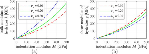51)–(54) requires expressions for the bulk and shear moduli of the hydrates, as functions of the indentation modulus. The latter is a function of the elastic stiffness properties of the nanoindentation-probed domain and of the diamond tip of the indenter. For an isotropic domain, this function reads as [8] (55) $$\frac{1}{M}=\frac{1-{\nu }_h^2}{E}+\frac{1-{0.07}^2}{1141\text{GPa}},$$(55) where E and ν_h denote the modulus of elasticity and Poisson’s ratio of the hydrates. Herein, ν_h is assumed to be constant.² In other words, the distribution of indentation modulus is related to a corresponding distribution of the modulus of elasticity, E. The latter distribution follows from solving Eq. (55)(55) $$\frac{1}{M}=\frac{1-{\nu }_h^2}{E}+\frac{1-{0.07}^2}{1141\text{GPa}},$$(55) for E: (56) $$E(M)=\frac{1-{\nu }_h^2}{\frac{1}{M}-\frac{1-{0.07}^2}{1141\text{GPa}}}.$$(56) The sought bulk moduli $k_i(M)$ and the shear moduli $g_i(M)$ follow from standard relations for isotropic elastic media: (57) $$k_i(M)=\frac{E(M)}{3(1-2{\nu }_h)},\hspace{1em}i=3,4,$$(57) (58) $$g_i(M)=\frac{E(M)}{2(1+{\nu }_h)},\hspace{1em}i=3,4,$$(58) see also Fig. 5.

Figure 5. (a) Bulk and (b) shear modulus of the hydrates as a function of the indentation modulus, for three different values of Poisson’s ratio of the hydrates.

2.7. Identification of crack density of Biodentine and Poisson’s ratio of hydrates

In order to identify the values of the crack density of Biodentine and of Poisson’s ratio of the hydrates, the search intervals $\omega =[0.5 ; 2.0]$ and ${\nu }_h=[0.15 ; 0.30]$ are subdivided into 7 equidistant values, defining a search grid. For all 49 combination of values (= grid points), $k_{\mathit{bio}}(\omega ,{\nu }_h)$ and $g_{\mathit{bio}}(\omega ,{\nu }_h)$ are computed according to Eqs. (41)(41) $$\begin{array}{c}{k}_{\mathit{bio}}=\{\sum _{i=1}^2\frac{f_i{k}_i}{1+\frac{S_{\mathit{vol}}(k_i-k_{\mathit{bio}})}{k_{\mathit{bio}}}}+\sum _{i=3}^4{f}_i\underset{0}{\overset{\infty }{\int }}\frac{{\phi }_i(M)k_i(M)}{1+\frac{S_{\mathit{vol}}(k_i(M)-k_{\mathit{bio}})}{k_{\mathit{bio}}}} \mathrm{d}M\}\\ \times {\{\sum _{i=1}^2\frac{f_i}{1+\frac{S_{\mathit{vol}}(k_i-k_{\mathit{bio}})}{k_{\mathit{bio}}}}+\sum _{i=3}^4{f}_i\mathrm{ }\underset{0}{\overset{\infty }{\int }}\frac{{\phi }_i(M)}{1+\frac{S_{\mathit{vol}}(k_i(M)-k_{\mathit{bio}})}{k_{\mathit{bio}}}} \mathrm{d}M\}}^{-1},\end{array}$$(41) and (42)(42) $$\begin{array}{c}{g}_{\mathit{bio}}=\{\sum _{i=1}^2\frac{f_i{g}_i}{1+\frac{S_{\mathit{dev}}(g_i-g_{\mathit{bio}})}{g_{\mathit{bio}}}}+\sum _{i=3}^4{f}_i\underset{0}{\overset{\infty }{\int }}\frac{{\phi }_i(M)g_i(M)}{1+\frac{S_{\mathit{dev}}(g_i(M)-g_{\mathit{bio}})}{g_{\mathit{bio}}}} \mathrm{d}M\}\\ \times \{\sum _{i=1}^2\frac{f_i}{1+\frac{S_{\mathit{dev}}(g_i-g_{\mathit{bio}})}{g_{\mathit{bio}}}}+\sum _{i=3}^4{f}_i\underset{0}{\overset{\infty }{\int }}\frac{{\phi }_i(M)}{1+\frac{S_{\mathit{dev}}(g_i(M)-g_{\mathit{bio}})}{g_{\mathit{bio}}}} \mathrm{d}M\\ \hspace{1em}+\frac{4\pi \omega }{3}{T}_{\mathit{dev}}{\}}^{-1}.\end{array}$$(42) . Because they are implicit expressions of the homogenized bulk and shear moduli of Biodentine, k_bio and g_bio are quantified iteratively, as outlined in the flowchart given in Table 3.

Table 3. Flowchart for the computation of k_bio and g_bio according to Eqs. (41)(41) $$\begin{array}{c}{k}_{\mathit{bio}}=\{\sum _{i=1}^2\frac{f_i{k}_i}{1+\frac{S_{\mathit{vol}}(k_i-k_{\mathit{bio}})}{k_{\mathit{bio}}}}+\sum _{i=3}^4{f}_i\underset{0}{\overset{\infty }{\int }}\frac{{\phi }_i(M)k_i(M)}{1+\frac{S_{\mathit{vol}}(k_i(M)-k_{\mathit{bio}})}{k_{\mathit{bio}}}} \mathrm{d}M\}\\ \times {\{\sum _{i=1}^2\frac{f_i}{1+\frac{S_{\mathit{vol}}(k_i-k_{\mathit{bio}})}{k_{\mathit{bio}}}}+\sum _{i=3}^4{f}_i\mathrm{ }\underset{0}{\overset{\infty }{\int }}\frac{{\phi }_i(M)}{1+\frac{S_{\mathit{vol}}(k_i(M)-k_{\mathit{bio}})}{k_{\mathit{bio}}}} \mathrm{d}M\}}^{-1},\end{array}$$(41) and (42)(42) $$\begin{array}{c}{g}_{\mathit{bio}}=\{\sum _{i=1}^2\frac{f_i{g}_i}{1+\frac{S_{\mathit{dev}}(g_i-g_{\mathit{bio}})}{g_{\mathit{bio}}}}+\sum _{i=3}^4{f}_i\underset{0}{\overset{\infty }{\int }}\frac{{\phi }_i(M)g_i(M)}{1+\frac{S_{\mathit{dev}}(g_i(M)-g_{\mathit{bio}})}{g_{\mathit{bio}}}} \mathrm{d}M\}\\ \times \{\sum _{i=1}^2\frac{f_i}{1+\frac{S_{\mathit{dev}}(g_i-g_{\mathit{bio}})}{g_{\mathit{bio}}}}+\sum _{i=3}^4{f}_i\underset{0}{\overset{\infty }{\int }}\frac{{\phi }_i(M)}{1+\frac{S_{\mathit{dev}}(g_i(M)-g_{\mathit{bio}})}{g_{\mathit{bio}}}} \mathrm{d}M\\ \hspace{1em}+\frac{4\pi \omega }{3}{T}_{\mathit{dev}}{\}}^{-1}.\end{array}$$(42) , respectively.

1.	Define numerical values of the crack density parameter ω and of Poisson’s ratio of the hydrates, νh.
2.	Define initial values of kbio and gbio as arbitrary positive numbers; for example, $k_{\mathit{bio}}=4.2\text{GPa}$ and $g_{\mathit{bio}}=2.5\text{GPa}.$
3.	Set the tolerance value tol equal to ${10}^{-10}.$
4.	Save kbio as $k_{\mathit{bio}}^{\mathit{old}}$ and gbio as $g_{\mathit{bio}}^{\mathit{old}}.$
5.	Compute Tdev, Svol, Sdev according to Eqs. (35)(35) $$T_{\mathit{dev}}=\frac{8(3k_{\mathit{bio}}+4g_{\mathit{bio}})}{15\pi (3k_{\mathit{bio}}+2g_{\mathit{bio}})}.$$(35) , (39)(39) $$S_{\mathit{vol}}=\frac{3k_{\mathit{bio}}}{3k_{\mathit{bio}}+4g_{\mathit{bio}}},$$(39) , (40)(40) $$S_{\mathit{dev}}=\frac{6(k_{\mathit{bio}}+2g_{\mathit{bio}})}{5(3k_{\mathit{bio}}+4g_{\mathit{bio}})}.$$(40) .
6.	Evaluate the integrals in Eqs. (41)(41) $$\begin{array}{c}{k}_{\mathit{bio}}=\{\sum _{i=1}^2\frac{f_i{k}_i}{1+\frac{S_{\mathit{vol}}(k_i-k_{\mathit{bio}})}{k_{\mathit{bio}}}}+\sum _{i=3}^4{f}_i\underset{0}{\overset{\infty }{\int }}\frac{{\phi }_i(M)k_i(M)}{1+\frac{S_{\mathit{vol}}(k_i(M)-k_{\mathit{bio}})}{k_{\mathit{bio}}}} \mathrm{d}M\}\\ \times {\{\sum _{i=1}^2\frac{f_i}{1+\frac{S_{\mathit{vol}}(k_i-k_{\mathit{bio}})}{k_{\mathit{bio}}}}+\sum _{i=3}^4{f}_i\mathrm{ }\underset{0}{\overset{\infty }{\int }}\frac{{\phi }_i(M)}{1+\frac{S_{\mathit{vol}}(k_i(M)-k_{\mathit{bio}})}{k_{\mathit{bio}}}} \mathrm{d}M\}}^{-1},\end{array}$$(41) and (42)(42) $$\begin{array}{c}{g}_{\mathit{bio}}=\{\sum _{i=1}^2\frac{f_i{g}_i}{1+\frac{S_{\mathit{dev}}(g_i-g_{\mathit{bio}})}{g_{\mathit{bio}}}}+\sum _{i=3}^4{f}_i\underset{0}{\overset{\infty }{\int }}\frac{{\phi }_i(M)g_i(M)}{1+\frac{S_{\mathit{dev}}(g_i(M)-g_{\mathit{bio}})}{g_{\mathit{bio}}}} \mathrm{d}M\}\\ \times \{\sum _{i=1}^2\frac{f_i}{1+\frac{S_{\mathit{dev}}(g_i-g_{\mathit{bio}})}{g_{\mathit{bio}}}}+\sum _{i=3}^4{f}_i\underset{0}{\overset{\infty }{\int }}\frac{{\phi }_i(M)}{1+\frac{S_{\mathit{dev}}(g_i(M)-g_{\mathit{bio}})}{g_{\mathit{bio}}}} \mathrm{d}M\\ \hspace{1em}+\frac{4\pi \omega }{3}{T}_{\mathit{dev}}{\}}^{-1}.\end{array}$$(42) based on ${\phi }_3(M)$ and ${\phi }_4(M)$ according to Eq. (19)(19) $${\phi }_i(M)=\frac{1}{M{\sigma }_i\sqrt{2\pi }}\hspace{0.17em}\text{exp}\hspace{0.17em}\mathrm{}(\mathrm{}-\frac{1}{2}{\left[\frac{\hspace{0.17em}\text{ln}\hspace{0.17em}(M)-{\mu }_i}{{\sigma }_i}\right]}^2),\hspace{1em}i=3,4.$$(19) with values of μ3, σ3, μ4, σ4 from Table 2, as well as $k_3(M),g_3(M),k_4(M),g_4(M)$ according to Eqs. (57)(57) $$k_i(M)=\frac{E(M)}{3(1-2{\nu }_h)},\hspace{1em}i=3,4,$$(57) and (58)(58) $$g_i(M)=\frac{E(M)}{2(1+{\nu }_h)},\hspace{1em}i=3,4,$$(58) , with E(M) according to Eq. (56)(56) $$E(M)=\frac{1-{\nu }_h^2}{\frac{1}{M}-\frac{1-{0.07}^2}{1141\text{GPa}}}.$$(56) .
7.	Evaluate the sums in Eqs. (41)(41) $$\begin{array}{c}{k}_{\mathit{bio}}=\{\sum _{i=1}^2\frac{f_i{k}_i}{1+\frac{S_{\mathit{vol}}(k_i-k_{\mathit{bio}})}{k_{\mathit{bio}}}}+\sum _{i=3}^4{f}_i\underset{0}{\overset{\infty }{\int }}\frac{{\phi }_i(M)k_i(M)}{1+\frac{S_{\mathit{vol}}(k_i(M)-k_{\mathit{bio}})}{k_{\mathit{bio}}}} \mathrm{d}M\}\\ \times {\{\sum _{i=1}^2\frac{f_i}{1+\frac{S_{\mathit{vol}}(k_i-k_{\mathit{bio}})}{k_{\mathit{bio}}}}+\sum _{i=3}^4{f}_i\mathrm{ }\underset{0}{\overset{\infty }{\int }}\frac{{\phi }_i(M)}{1+\frac{S_{\mathit{vol}}(k_i(M)-k_{\mathit{bio}})}{k_{\mathit{bio}}}} \mathrm{d}M\}}^{-1},\end{array}$$(41) and (42)(42) $$\begin{array}{c}{g}_{\mathit{bio}}=\{\sum _{i=1}^2\frac{f_i{g}_i}{1+\frac{S_{\mathit{dev}}(g_i-g_{\mathit{bio}})}{g_{\mathit{bio}}}}+\sum _{i=3}^4{f}_i\underset{0}{\overset{\infty }{\int }}\frac{{\phi }_i(M)g_i(M)}{1+\frac{S_{\mathit{dev}}(g_i(M)-g_{\mathit{bio}})}{g_{\mathit{bio}}}} \mathrm{d}M\}\\ \times \{\sum _{i=1}^2\frac{f_i}{1+\frac{S_{\mathit{dev}}(g_i-g_{\mathit{bio}})}{g_{\mathit{bio}}}}+\sum _{i=3}^4{f}_i\underset{0}{\overset{\infty }{\int }}\frac{{\phi }_i(M)}{1+\frac{S_{\mathit{dev}}(g_i(M)-g_{\mathit{bio}})}{g_{\mathit{bio}}}} \mathrm{d}M\\ \hspace{1em}+\frac{4\pi \omega }{3}{T}_{\mathit{dev}}{\}}^{-1}.\end{array}$$(42) based on f1, f2, f3, f4, k1, g1, k2, g2 from Table 2.
8.	Quantify kbio and gbio according to Eqs. (41)(41) $$\begin{array}{c}{k}_{\mathit{bio}}=\{\sum _{i=1}^2\frac{f_i{k}_i}{1+\frac{S_{\mathit{vol}}(k_i-k_{\mathit{bio}})}{k_{\mathit{bio}}}}+\sum _{i=3}^4{f}_i\underset{0}{\overset{\infty }{\int }}\frac{{\phi }_i(M)k_i(M)}{1+\frac{S_{\mathit{vol}}(k_i(M)-k_{\mathit{bio}})}{k_{\mathit{bio}}}} \mathrm{d}M\}\\ \times {\{\sum _{i=1}^2\frac{f_i}{1+\frac{S_{\mathit{vol}}(k_i-k_{\mathit{bio}})}{k_{\mathit{bio}}}}+\sum _{i=3}^4{f}_i\mathrm{ }\underset{0}{\overset{\infty }{\int }}\frac{{\phi }_i(M)}{1+\frac{S_{\mathit{vol}}(k_i(M)-k_{\mathit{bio}})}{k_{\mathit{bio}}}} \mathrm{d}M\}}^{-1},\end{array}$$(41) and (42)(42) $$\begin{array}{c}{g}_{\mathit{bio}}=\{\sum _{i=1}^2\frac{f_i{g}_i}{1+\frac{S_{\mathit{dev}}(g_i-g_{\mathit{bio}})}{g_{\mathit{bio}}}}+\sum _{i=3}^4{f}_i\underset{0}{\overset{\infty }{\int }}\frac{{\phi }_i(M)g_i(M)}{1+\frac{S_{\mathit{dev}}(g_i(M)-g_{\mathit{bio}})}{g_{\mathit{bio}}}} \mathrm{d}M\}\\ \times \{\sum _{i=1}^2\frac{f_i}{1+\frac{S_{\mathit{dev}}(g_i-g_{\mathit{bio}})}{g_{\mathit{bio}}}}+\sum _{i=3}^4{f}_i\underset{0}{\overset{\infty }{\int }}\frac{{\phi }_i(M)}{1+\frac{S_{\mathit{dev}}(g_i(M)-g_{\mathit{bio}})}{g_{\mathit{bio}}}} \mathrm{d}M\\ \hspace{1em}+\frac{4\pi \omega }{3}{T}_{\mathit{dev}}{\}}^{-1}.\end{array}$$(42) .
9.	Determine the convergence ratio according to $c=\frac{\Vert k_{\mathit{bio}}-k_{\mathit{bio}}^{\mathit{old}}\Vert }{k_{\mathit{bio}}^{\mathit{old}}}+\frac{\Vert g_{\mathit{bio}}-g_{\mathit{bio}}^{\mathit{old}}\Vert }{g_{\mathit{bio}}^{\mathit{old}}}.$
10.	If c < tol then stop the iteration; else go to 4. (= start the next iteration step).

For every grid point, the square root of the sum of squared errors is quantified based on the computed homogenized stiffness moduli and their experimental counterparts, see the ultrasonics-derived values in Eqs. (1)(1) $$k_{\mathit{bio}}^{\hspace{0.17em}\mathit{\text{exp}}\hspace{0.17em}}=38.4\text{GPa},$$(1) and (2)(2) $$g_{\mathit{bio}}^{\hspace{0.17em}\mathit{\text{exp}}\hspace{0.17em}}=14.1\text{GPa},$$(2) : (59) $${\epsilon }_{\mathit{SRSS}}=\sqrt{{[k_{\mathit{bio}}^{\hspace{0.17em}\text{exp}\hspace{0.17em}}-k_{\mathit{bio}}(\omega ,{\nu }_h)]}^2+{[g_{\mathit{bio}}^{\hspace{0.17em}\text{exp}\hspace{0.17em}}-g_{\mathit{bio}}(\omega ,{\nu }_h)]}^2}.$$(59) The obtained error surface exhibits one minimum in the vicinity of $\omega \approx 0.78$ and ${\nu }_h\approx 0.20,$ see also Fig. 6. The optimal solution is found iteratively, using a method based on search intervals which are progressively refined and shifted, see [3, 33]. The lognormal microelasticity model reproduces the ultrasonics-derived macrostiffness moduli when using the following values of the crack density parameter and of Poisson’s ratio of LDCR and HDCR hydrates as input: (60) $$\omega =0.7802,$$(60) (61) $${\nu }_h=0.2017,$$(61) see also Fig. 7. The numerical values of the integrals in Eqs. (41)(41) $$\begin{array}{c}{k}_{\mathit{bio}}=\{\sum _{i=1}^2\frac{f_i{k}_i}{1+\frac{S_{\mathit{vol}}(k_i-k_{\mathit{bio}})}{k_{\mathit{bio}}}}+\sum _{i=3}^4{f}_i\underset{0}{\overset{\infty }{\int }}\frac{{\phi }_i(M)k_i(M)}{1+\frac{S_{\mathit{vol}}(k_i(M)-k_{\mathit{bio}})}{k_{\mathit{bio}}}} \mathrm{d}M\}\\ \times {\{\sum _{i=1}^2\frac{f_i}{1+\frac{S_{\mathit{vol}}(k_i-k_{\mathit{bio}})}{k_{\mathit{bio}}}}+\sum _{i=3}^4{f}_i\mathrm{ }\underset{0}{\overset{\infty }{\int }}\frac{{\phi }_i(M)}{1+\frac{S_{\mathit{vol}}(k_i(M)-k_{\mathit{bio}})}{k_{\mathit{bio}}}} \mathrm{d}M\}}^{-1},\end{array}$$(41) , (42)(42) $$\begin{array}{c}{g}_{\mathit{bio}}=\{\sum _{i=1}^2\frac{f_i{g}_i}{1+\frac{S_{\mathit{dev}}(g_i-g_{\mathit{bio}})}{g_{\mathit{bio}}}}+\sum _{i=3}^4{f}_i\underset{0}{\overset{\infty }{\int }}\frac{{\phi }_i(M)g_i(M)}{1+\frac{S_{\mathit{dev}}(g_i(M)-g_{\mathit{bio}})}{g_{\mathit{bio}}}} \mathrm{d}M\}\\ \times \{\sum _{i=1}^2\frac{f_i}{1+\frac{S_{\mathit{dev}}(g_i-g_{\mathit{bio}})}{g_{\mathit{bio}}}}+\sum _{i=3}^4{f}_i\underset{0}{\overset{\infty }{\int }}\frac{{\phi }_i(M)}{1+\frac{S_{\mathit{dev}}(g_i(M)-g_{\mathit{bio}})}{g_{\mathit{bio}}}} \mathrm{d}M\\ \hspace{1em}+\frac{4\pi \omega }{3}{T}_{\mathit{dev}}{\}}^{-1}.\end{array}$$(42) and (44)–(47), obtained with $k_{\mathit{bio}}=38.4\text{GPa},g_{\mathit{bio}}=14.1\text{GPa},$ and ${\nu }_h=0.2017,$ are listed in Appendix B.

Figure 6. Square root of the sum of squared errors (59), quantifying the difference between computed homogenized stiffness moduli, see Eqs. (41)(41) $$\begin{array}{c}{k}_{\mathit{bio}}=\{\sum _{i=1}^2\frac{f_i{k}_i}{1+\frac{S_{\mathit{vol}}(k_i-k_{\mathit{bio}})}{k_{\mathit{bio}}}}+\sum _{i=3}^4{f}_i\underset{0}{\overset{\infty }{\int }}\frac{{\phi }_i(M)k_i(M)}{1+\frac{S_{\mathit{vol}}(k_i(M)-k_{\mathit{bio}})}{k_{\mathit{bio}}}} \mathrm{d}M\}\\ \times {\{\sum _{i=1}^2\frac{f_i}{1+\frac{S_{\mathit{vol}}(k_i-k_{\mathit{bio}})}{k_{\mathit{bio}}}}+\sum _{i=3}^4{f}_i\mathrm{ }\underset{0}{\overset{\infty }{\int }}\frac{{\phi }_i(M)}{1+\frac{S_{\mathit{vol}}(k_i(M)-k_{\mathit{bio}})}{k_{\mathit{bio}}}} \mathrm{d}M\}}^{-1},\end{array}$$(41) and (42)(42) $$\begin{array}{c}{g}_{\mathit{bio}}=\{\sum _{i=1}^2\frac{f_i{g}_i}{1+\frac{S_{\mathit{dev}}(g_i-g_{\mathit{bio}})}{g_{\mathit{bio}}}}+\sum _{i=3}^4{f}_i\underset{0}{\overset{\infty }{\int }}\frac{{\phi }_i(M)g_i(M)}{1+\frac{S_{\mathit{dev}}(g_i(M)-g_{\mathit{bio}})}{g_{\mathit{bio}}}} \mathrm{d}M\}\\ \times \{\sum _{i=1}^2\frac{f_i}{1+\frac{S_{\mathit{dev}}(g_i-g_{\mathit{bio}})}{g_{\mathit{bio}}}}+\sum _{i=3}^4{f}_i\underset{0}{\overset{\infty }{\int }}\frac{{\phi }_i(M)}{1+\frac{S_{\mathit{dev}}(g_i(M)-g_{\mathit{bio}})}{g_{\mathit{bio}}}} \mathrm{d}M\\ \hspace{1em}+\frac{4\pi \omega }{3}{T}_{\mathit{dev}}{\}}^{-1}.\end{array}$$(42) as well as Table 3, and their experimental counterparts, see Eqs. (1)(1) $$k_{\mathit{bio}}^{\hspace{0.17em}\mathit{\text{exp}}\hspace{0.17em}}=38.4\text{GPa},$$(1) and (2)(2) $$g_{\mathit{bio}}^{\hspace{0.17em}\mathit{\text{exp}}\hspace{0.17em}}=14.1\text{GPa},$$(2) .

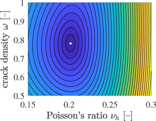
Figure 7. Homogenized stiffness moduli k_bio and g_bio according to Eqs. (41)(41) $$\begin{array}{c}{k}_{\mathit{bio}}=\{\sum _{i=1}^2\frac{f_i{k}_i}{1+\frac{S_{\mathit{vol}}(k_i-k_{\mathit{bio}})}{k_{\mathit{bio}}}}+\sum _{i=3}^4{f}_i\underset{0}{\overset{\infty }{\int }}\frac{{\phi }_i(M)k_i(M)}{1+\frac{S_{\mathit{vol}}(k_i(M)-k_{\mathit{bio}})}{k_{\mathit{bio}}}} \mathrm{d}M\}\\ \times {\{\sum _{i=1}^2\frac{f_i}{1+\frac{S_{\mathit{vol}}(k_i-k_{\mathit{bio}})}{k_{\mathit{bio}}}}+\sum _{i=3}^4{f}_i\mathrm{ }\underset{0}{\overset{\infty }{\int }}\frac{{\phi }_i(M)}{1+\frac{S_{\mathit{vol}}(k_i(M)-k_{\mathit{bio}})}{k_{\mathit{bio}}}} \mathrm{d}M\}}^{-1},\end{array}$$(41) and (42)(42) $$\begin{array}{c}{g}_{\mathit{bio}}=\{\sum _{i=1}^2\frac{f_i{g}_i}{1+\frac{S_{\mathit{dev}}(g_i-g_{\mathit{bio}})}{g_{\mathit{bio}}}}+\sum _{i=3}^4{f}_i\underset{0}{\overset{\infty }{\int }}\frac{{\phi }_i(M)g_i(M)}{1+\frac{S_{\mathit{dev}}(g_i(M)-g_{\mathit{bio}})}{g_{\mathit{bio}}}} \mathrm{d}M\}\\ \times \{\sum _{i=1}^2\frac{f_i}{1+\frac{S_{\mathit{dev}}(g_i-g_{\mathit{bio}})}{g_{\mathit{bio}}}}+\sum _{i=3}^4{f}_i\underset{0}{\overset{\infty }{\int }}\frac{{\phi }_i(M)}{1+\frac{S_{\mathit{dev}}(g_i(M)-g_{\mathit{bio}})}{g_{\mathit{bio}}}} \mathrm{d}M\\ \hspace{1em}+\frac{4\pi \omega }{3}{T}_{\mathit{dev}}{\}}^{-1}.\end{array}$$(42) , as functions of the crack density of Biodentine and Poisson’s ratio of the hydrates, see the solid blue lines, and ultrasonics-derived counterparts according to Eqs. (1)(1) $$k_{\mathit{bio}}^{\hspace{0.17em}\mathit{\text{exp}}\hspace{0.17em}}=38.4\text{GPa},$$(1) and (2)(2) $$g_{\mathit{bio}}^{\hspace{0.17em}\mathit{\text{exp}}\hspace{0.17em}}=14.1\text{GPa},$$(2) , see the red dashed lines; the circles mark the optimal solutions, see also Eqs. (60)(60) $$\omega =0.7802,$$(60) and (61)(61) $${\nu }_h=0.2017,$$(61) .

3. Application of the lognormal microelasticity model: strain and stress fluctuations

3.1. Distributions of strain concentration tensor components of the two populations of hydrates

Probability distribution functions for strain concentration tensor components of both populations of hydrates are computed as follows. Eq. (19)(19) $${\phi }_i(M)=\frac{1}{M{\sigma }_i\sqrt{2\pi }}\hspace{0.17em}\text{exp}\hspace{0.17em}\mathrm{}(\mathrm{}-\frac{1}{2}{\left[\frac{\hspace{0.17em}\text{ln}\hspace{0.17em}(M)-{\mu }_i}{{\sigma }_i}\right]}^2),\hspace{1em}i=3,4.$$(19) provides access to the probability density as a function of the indentation modulus. Eqs. (46)(46) $$\begin{array}{c}{A}_{\mathit{vol},i}(M)=\frac{1}{1+\frac{S_{\mathit{vol}}(k_i(M)-k_{\mathit{bio}})}{k_{\mathit{bio}}}}\{\sum _{i=1}^2\frac{f_i}{1+\frac{S_{\mathit{vol}}(k_i-k_{\mathit{bio}})}{k_{\mathit{bio}}}}\\ +\sum _{i=3}^4{f}_i\mathrm{ }\underset{0}{\overset{\infty }{\int }}\frac{{\phi }_i(M)}{1+\frac{S_{\mathit{vol}}(k_i(M)-k_{\mathit{bio}})}{k_{\mathit{bio}}}} \mathrm{d}M{\}}^{-1},\end{array}$$(46) and (47)(47) $$\begin{array}{c}{A}_{\mathit{dev},i}(M)=\frac{1}{1+\frac{S_{\mathit{dev}}(g_i(M)-g_{\mathit{bio}})}{g_{\mathit{bio}}}}\{\sum _{i=1}^2\frac{f_i}{1+\frac{S_{\mathit{dev}}(g_i-g_{\mathit{bio}})}{g_{\mathit{bio}}}}\\ +\sum _{i=3}^4{f}_i\underset{0}{\overset{\infty }{\int }}\mathrm{ }\frac{{\phi }_i(M)}{1+\frac{S_{\mathit{dev}}(g_i(M)-g_{\mathit{bio}})}{g_{\mathit{bio}}}} \mathrm{d}M+\frac{4\pi \omega }{3}{T}_{\mathit{dev}}{\}}^{-1},\end{array}$$(47) allow for computing the volumetric and deviatoric components of the strain concentration tensor as a function of the indentation modulus. Combining Eq. (19)(19) $${\phi }_i(M)=\frac{1}{M{\sigma }_i\sqrt{2\pi }}\hspace{0.17em}\text{exp}\hspace{0.17em}\mathrm{}(\mathrm{}-\frac{1}{2}{\left[\frac{\hspace{0.17em}\text{ln}\hspace{0.17em}(M)-{\mu }_i}{{\sigma }_i}\right]}^2),\hspace{1em}i=3,4.$$(19) with Eq. (46)(46) $$\begin{array}{c}{A}_{\mathit{vol},i}(M)=\frac{1}{1+\frac{S_{\mathit{vol}}(k_i(M)-k_{\mathit{bio}})}{k_{\mathit{bio}}}}\{\sum _{i=1}^2\frac{f_i}{1+\frac{S_{\mathit{vol}}(k_i-k_{\mathit{bio}})}{k_{\mathit{bio}}}}\\ +\sum _{i=3}^4{f}_i\mathrm{ }\underset{0}{\overset{\infty }{\int }}\frac{{\phi }_i(M)}{1+\frac{S_{\mathit{vol}}(k_i(M)-k_{\mathit{bio}})}{k_{\mathit{bio}}}} \mathrm{d}M{\}}^{-1},\end{array}$$(46) and Eq. (47)(47) $$\begin{array}{c}{A}_{\mathit{dev},i}(M)=\frac{1}{1+\frac{S_{\mathit{dev}}(g_i(M)-g_{\mathit{bio}})}{g_{\mathit{bio}}}}\{\sum _{i=1}^2\frac{f_i}{1+\frac{S_{\mathit{dev}}(g_i-g_{\mathit{bio}})}{g_{\mathit{bio}}}}\\ +\sum _{i=3}^4{f}_i\underset{0}{\overset{\infty }{\int }}\mathrm{ }\frac{{\phi }_i(M)}{1+\frac{S_{\mathit{dev}}(g_i(M)-g_{\mathit{bio}})}{g_{\mathit{bio}}}} \mathrm{d}M+\frac{4\pi \omega }{3}{T}_{\mathit{dev}}{\}}^{-1},\end{array}$$(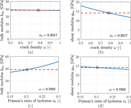47) , respectively, allows for producing parametric plots showing probability density over strain concentration tensor components, with the indentation modulus as the parameter. Normalizing the obtained parametric plots such that the area under the graphs becomes equal to 1, delivers probability density functions for the strain concentration tensor components, see Fig. 8. The probability densities of A_vol and A_dev of the LDCR hydrates are left-skewed functions. The corresponding results obtained for the HDCR hydrates, in turn, are reminiscent of Gaussian distributions.

Figure 8. Results of the lognormal microelasticity model (black graphs): statistical distributions of volumetric and deviatoric components of the strain concentration tensors of LDCR hydrates and of HDCR hydrates: (a) and (c) show probability density distributions, (b) and (d) cumulative distribution functions. The best fits of generalized beta-distributions to the statistical distributions are the red dashed graphs, see Eqs. (70)(70) $${\phi }_i^B(y)=\frac{{\left(\frac{y-a}{c-a}\right)}^{\alpha -1}{\left(\frac{c-y}{c-a}\right)}^{\beta -1}}{(c-a)\times B(\alpha ,\beta )},$$(70) and (71)(71) $$B(\alpha ,\beta )=\frac{\Gamma (\alpha )\Gamma (\beta )}{\Gamma (\alpha +\beta )},$$(71) as well as the Beta distributions parameters listed in Table 6.

It is interesting to quantify the strain concentration tensor components averaged over each one of the two populations of hydrates. Notably, the volume average rule applies for strain concentration tensors [26]. Thus, the population-averaged volumetric and deviatoric strain concentration tensor components read as (62) $${\overline{A_{\mathit{vol}}}}_{,j}=\mathrm{ }\underset{0}{\overset{\infty }{\int }}{\phi }_j(M)A_{\mathit{vol},j}(M) \mathrm{d}M\mathrm{\hspace{1em}}\mathrm{\hspace{1em}}j=3,4,$$(62) (63) $${\overline{A_{\mathit{dev}}}}_{,j}=\underset{0}{\overset{\infty }{\int }}{\phi }_j(M)A_{\mathit{dev},j}(M) \mathrm{d}M\mathrm{\hspace{1em}}\mathrm{\hspace{1em}}j=3,4.$$(63) Inserting $A_{\mathit{vol},j}(M)$ and $A_{\mathit{dev},j}(M)$ according to Eqs. (46)(46) $$\begin{array}{c}{A}_{\mathit{vol},i}(M)=\frac{1}{1+\frac{S_{\mathit{vol}}(k_i(M)-k_{\mathit{bio}})}{k_{\mathit{bio}}}}\{\sum _{i=1}^2\frac{f_i}{1+\frac{S_{\mathit{vol}}(k_i-k_{\mathit{bio}})}{k_{\mathit{bio}}}}\\ +\sum _{i=3}^4{f}_i\mathrm{ }\underset{0}{\overset{\infty }{\int }}\frac{{\phi }_i(M)}{1+\frac{S_{\mathit{vol}}(k_i(M)-k_{\mathit{bio}})}{k_{\mathit{bio}}}} \mathrm{d}M{\}}^{-1},\end{array}$$(46) and (47)(47) $$\begin{array}{c}{A}_{\mathit{dev},i}(M)=\frac{1}{1+\frac{S_{\mathit{dev}}(g_i(M)-g_{\mathit{bio}})}{g_{\mathit{bio}}}}\{\sum _{i=1}^2\frac{f_i}{1+\frac{S_{\mathit{dev}}(g_i-g_{\mathit{bio}})}{g_{\mathit{bio}}}}\\ +\sum _{i=3}^4{f}_i\underset{0}{\overset{\infty }{\int }}\mathrm{ }\frac{{\phi }_i(M)}{1+\frac{S_{\mathit{dev}}(g_i(M)-g_{\mathit{bio}})}{g_{\mathit{bio}}}} \mathrm{d}M+\frac{4\pi \omega }{3}{T}_{\mathit{dev}}{\}}^{-1},\end{array}$$(47) , respectively, into Eqs. (62)(62) $${\overline{A_{\mathit{vol}}}}_{,j}=\mathrm{ }\underset{0}{\overset{\infty }{\int }}{\phi }_j(M)A_{\mathit{vol},j}(M) \mathrm{d}M\mathrm{\hspace{1em}}\mathrm{\hspace{1em}}j=3,4,$$(62) and (63)(63) $${\overline{A_{\mathit{dev}}}}_{,j}=\underset{0}{\overset{\infty }{\int }}{\phi }_j(M)A_{\mathit{dev},j}(M) \mathrm{d}M\mathrm{\hspace{1em}}\mathrm{\hspace{1em}}j=3,4.$$(63) yields (64) $$\begin{array}{c}\overline{A_{\mathit{vol},j}}=\underset{0}{\overset{\infty }{\int }}\frac{{\phi }_j(M)}{1+\frac{S_{\mathit{vol}}(k_j(M)-k_{\mathit{bio}})}{k_{\mathit{bio}}}} \mathrm{d}M\\ \times {\{\sum _{i=1}^2\frac{f_i}{1+\frac{S_{\mathit{vol}}(k_i-k_{\mathit{bio}})}{k_{\mathit{bio}}}}+\sum _{i=3}^4{f}_i\mathrm{ }\underset{0}{\overset{\infty }{\int }}\frac{{\phi }_i(M)}{1+\frac{S_{\mathit{vol}}(k_i(M)-k_{\mathit{bio}})}{k_{\mathit{bio}}}} \mathrm{d}M\}}^{-1},\end{array}$$(64) (65) $$\begin{array}{c}\overline{A_{\mathit{dev},j}}=\underset{0}{\overset{\infty }{\int }}\frac{{\phi }_j(M)}{1+\frac{S_{\mathit{dev}}(g_j(M)-g_{\mathit{bio}})}{g_{\mathit{bio}}}} \mathrm{d}M\\ \times \{\sum _{i=1}^2\frac{f_i}{1+\frac{S_{\mathit{dev}}(g_i-g_{\mathit{bio}})}{g_{\mathit{bio}}}}+\sum _{i=3}^4{f}_i\mathrm{ }\underset{0}{\overset{\infty }{\int }}\frac{{\phi }_i(M)}{1+\frac{S_{\mathit{dev}}(g_i(M)-g_{\mathit{bio}})}{g_{\mathit{bio}}}} \mathrm{d}M+\frac{4\pi \omega }{3}{T}_{\mathit{dev}}{\}}^{-1}.\end{array}$$(65) Evaluation of the strain concentration tensor components A_vol and A_dev of zirconia and clinker according to Eqs. (44)(44) $$\begin{array}{c}{A}_{\mathit{vol},i}=\frac{1}{1+\frac{S_{\mathit{vol}}(k_i-k_{\mathit{bio}})}{k_{\mathit{bio}}}}\{\sum _{i=1}^2\frac{f_i}{1+\frac{S_{\mathit{vol}}(k_i-k_{\mathit{bio}})}{k_{\mathit{bio}}}}\\ +\sum _{i=3}^4{f}_i\mathrm{ }\underset{0}{\overset{\infty }{\int }}\frac{{\phi }_i(M)}{1+\frac{S_{\mathit{vol}}(k_i(M)-k_{\mathit{bio}})}{k_{\mathit{bio}}}} \mathrm{d}M{\}}^{-1},\end{array}$$(44) and (45)(45) $$\begin{array}{c}{A}_{\mathit{dev},i}=\frac{1}{1+\frac{S_{\mathit{dev}}(g_i-g_{\mathit{bio}})}{g_{\mathit{bio}}}}\{\sum _{i=1}^2\frac{f_i}{1+\frac{S_{\mathit{dev}}(g_i-g_{\mathit{bio}})}{g_{\mathit{bio}}}}\\ +\sum _{i=3}^4{f}_i\mathrm{ }\underset{0}{\overset{\infty }{\int }}\frac{{\phi }_i(M)}{1+\frac{S_{\mathit{dev}}(g_i(M)-g_{\mathit{bio}})}{g_{\mathit{bio}}}} \mathrm{d}M+\frac{4\pi \omega }{3}{T}_{\mathit{dev}}{\}}^{-1}.\end{array}$$(45) , as well as the average strain concentration tensor components $\overline{A_{\mathit{vol}}}$ and $\overline{A_{\mathit{dev}}}$ of HDCR and LDCR hydrates according to Eqs. (64)(64) $$\begin{array}{c}\overline{A_{\mathit{vol},j}}=\underset{0}{\overset{\infty }{\int }}\frac{{\phi }_j(M)}{1+\frac{S_{\mathit{vol}}(k_j(M)-k_{\mathit{bio}})}{k_{\mathit{bio}}}} \mathrm{d}M\\ \times {\{\sum _{i=1}^2\frac{f_i}{1+\frac{S_{\mathit{vol}}(k_i-k_{\mathit{bio}})}{k_{\mathit{bio}}}}+\sum _{i=3}^4{f}_i\mathrm{ }\underset{0}{\overset{\infty }{\int }}\frac{{\phi }_i(M)}{1+\frac{S_{\mathit{vol}}(k_i(M)-k_{\mathit{bio}})}{k_{\mathit{bio}}}} \mathrm{d}M\}}^{-1},\end{array}$$(64) and (65)(65) $$\begin{array}{c}\overline{A_{\mathit{dev},j}}=\underset{0}{\overset{\infty }{\int }}\frac{{\phi }_j(M)}{1+\frac{S_{\mathit{dev}}(g_j(M)-g_{\mathit{bio}})}{g_{\mathit{bio}}}} \mathrm{d}M\\ \times \{\sum _{i=1}^2\frac{f_i}{1+\frac{S_{\mathit{dev}}(g_i-g_{\mathit{bio}})}{g_{\mathit{bio}}}}+\sum _{i=3}^4{f}_i\mathrm{ }\underset{0}{\overset{\infty }{\int }}\frac{{\phi }_i(M)}{1+\frac{S_{\mathit{dev}}(g_i(M)-g_{\mathit{bio}})}{g_{\mathit{bio}}}} \mathrm{d}M+\frac{4\pi \omega }{3}{T}_{\mathit{dev}}{\}}^{-1}.\end{array}$$(65) , yields numerical values listed in Table 4. These values quantify the expected trend that the strains experienced by the material constituents increase with decreasing stiffness.

Table 4. Results of the lognormal microelasticity model: (population-averaged) strain concentration tensors components of the four types of solid constituents of Biodentine.

Constituent of Biodentine	(Average) strain concentration tensor components		Source
zirconia	$A_{\mathit{vol},1}=0.3017$	$A_{\mathit{dev},1}=0.2352$	Eqs. (44)(44) $$\begin{array}{c}{A}_{\mathit{vol},i}=\frac{1}{1+\frac{S_{\mathit{vol}}(k_i-k_{\mathit{bio}})}{k_{\mathit{bio}}}}\{\sum _{i=1}^2\frac{f_i}{1+\frac{S_{\mathit{vol}}(k_i-k_{\mathit{bio}})}{k_{\mathit{bio}}}}\\ +\sum _{i=3}^4{f}_i\mathrm{ }\underset{0}{\overset{\infty }{\int }}\frac{{\phi }_i(M)}{1+\frac{S_{\mathit{vol}}(k_i(M)-k_{\mathit{bio}})}{k_{\mathit{bio}}}} \mathrm{d}M{\}}^{-1},\end{array}$$(44) and (45)(45) $$\begin{array}{c}{A}_{\mathit{dev},i}=\frac{1}{1+\frac{S_{\mathit{dev}}(g_i-g_{\mathit{bio}})}{g_{\mathit{bio}}}}\{\sum _{i=1}^2\frac{f_i}{1+\frac{S_{\mathit{dev}}(g_i-g_{\mathit{bio}})}{g_{\mathit{bio}}}}\\ +\sum _{i=3}^4{f}_i\mathrm{ }\underset{0}{\overset{\infty }{\int }}\frac{{\phi }_i(M)}{1+\frac{S_{\mathit{dev}}(g_i(M)-g_{\mathit{bio}})}{g_{\mathit{bio}}}} \mathrm{d}M+\frac{4\pi \omega }{3}{T}_{\mathit{dev}}{\}}^{-1}.\end{array}$$(45)
clinker	$A_{\mathit{vol},2}=0.4223$	$A_{\mathit{dev},2}=0.3192$	Eqs. (44)(44) $$\begin{array}{c}{A}_{\mathit{vol},i}=\frac{1}{1+\frac{S_{\mathit{vol}}(k_i-k_{\mathit{bio}})}{k_{\mathit{bio}}}}\{\sum _{i=1}^2\frac{f_i}{1+\frac{S_{\mathit{vol}}(k_i-k_{\mathit{bio}})}{k_{\mathit{bio}}}}\\ +\sum _{i=3}^4{f}_i\mathrm{ }\underset{0}{\overset{\infty }{\int }}\frac{{\phi }_i(M)}{1+\frac{S_{\mathit{vol}}(k_i(M)-k_{\mathit{bio}})}{k_{\mathit{bio}}}} \mathrm{d}M{\}}^{-1},\end{array}$$(44) and (45)(45) $$\begin{array}{c}{A}_{\mathit{dev},i}=\frac{1}{1+\frac{S_{\mathit{dev}}(g_i-g_{\mathit{bio}})}{g_{\mathit{bio}}}}\{\sum _{i=1}^2\frac{f_i}{1+\frac{S_{\mathit{dev}}(g_i-g_{\mathit{bio}})}{g_{\mathit{bio}}}}\\ +\sum _{i=3}^4{f}_i\mathrm{ }\underset{0}{\overset{\infty }{\int }}\frac{{\phi }_i(M)}{1+\frac{S_{\mathit{dev}}(g_i(M)-g_{\mathit{bio}})}{g_{\mathit{bio}}}} \mathrm{d}M+\frac{4\pi \omega }{3}{T}_{\mathit{dev}}{\}}^{-1}.\end{array}$$(45)
HDCR hydrates	${\overline{A_{\mathit{vol}}}}_{,3}=1.0551$	${\overline{A_{\mathit{dev}}}}_{,3}=0.5248$	Eqs. (64)(64) $$\begin{array}{c}\overline{A_{\mathit{vol},j}}=\underset{0}{\overset{\infty }{\int }}\frac{{\phi }_j(M)}{1+\frac{S_{\mathit{vol}}(k_j(M)-k_{\mathit{bio}})}{k_{\mathit{bio}}}} \mathrm{d}M\\ \times {\{\sum _{i=1}^2\frac{f_i}{1+\frac{S_{\mathit{vol}}(k_i-k_{\mathit{bio}})}{k_{\mathit{bio}}}}+\sum _{i=3}^4{f}_i\mathrm{ }\underset{0}{\overset{\infty }{\int }}\frac{{\phi }_i(M)}{1+\frac{S_{\mathit{vol}}(k_i(M)-k_{\mathit{bio}})}{k_{\mathit{bio}}}} \mathrm{d}M\}}^{-1},\end{array}$$(64) and (65)(65) $$\begin{array}{c}\overline{A_{\mathit{dev},j}}=\underset{0}{\overset{\infty }{\int }}\frac{{\phi }_j(M)}{1+\frac{S_{\mathit{dev}}(g_j(M)-g_{\mathit{bio}})}{g_{\mathit{bio}}}} \mathrm{d}M\\ \times \{\sum _{i=1}^2\frac{f_i}{1+\frac{S_{\mathit{dev}}(g_i-g_{\mathit{bio}})}{g_{\mathit{bio}}}}+\sum _{i=3}^4{f}_i\mathrm{ }\underset{0}{\overset{\infty }{\int }}\frac{{\phi }_i(M)}{1+\frac{S_{\mathit{dev}}(g_i(M)-g_{\mathit{bio}})}{g_{\mathit{bio}}}} \mathrm{d}M+\frac{4\pi \omega }{3}{T}_{\mathit{dev}}{\}}^{-1}.\end{array}$$(65)
LDCR hydrates	${\overline{A_{\mathit{vol}}}}_{,4}=1.3207$	${\overline{A_{\mathit{dev}}}}_{,4}=0.6428$	Eqs. (64)(64) $$\begin{array}{c}\overline{A_{\mathit{vol},j}}=\underset{0}{\overset{\infty }{\int }}\frac{{\phi }_j(M)}{1+\frac{S_{\mathit{vol}}(k_j(M)-k_{\mathit{bio}})}{k_{\mathit{bio}}}} \mathrm{d}M\\ \times {\{\sum _{i=1}^2\frac{f_i}{1+\frac{S_{\mathit{vol}}(k_i-k_{\mathit{bio}})}{k_{\mathit{bio}}}}+\sum _{i=3}^4{f}_i\mathrm{ }\underset{0}{\overset{\infty }{\int }}\frac{{\phi }_i(M)}{1+\frac{S_{\mathit{vol}}(k_i(M)-k_{\mathit{bio}})}{k_{\mathit{bio}}}} \mathrm{d}M\}}^{-1},\end{array}$$(64) and (65)(65) $$\begin{array}{c}\overline{A_{\mathit{dev},j}}=\underset{0}{\overset{\infty }{\int }}\frac{{\phi }_j(M)}{1+\frac{S_{\mathit{dev}}(g_j(M)-g_{\mathit{bio}})}{g_{\mathit{bio}}}} \mathrm{d}M\\ \times \{\sum _{i=1}^2\frac{f_i}{1+\frac{S_{\mathit{dev}}(g_i-g_{\mathit{bio}})}{g_{\mathit{bio}}}}+\sum _{i=3}^4{f}_i\mathrm{ }\underset{0}{\overset{\infty }{\int }}\frac{{\phi }_i(M)}{1+\frac{S_{\mathit{dev}}(g_i(M)-g_{\mathit{bio}})}{g_{\mathit{bio}}}} \mathrm{d}M+\frac{4\pi \omega }{3}{T}_{\mathit{dev}}{\}}^{-1}.\end{array}$$(65)

3.2. Distributions of stress concentration tensor components of the two populations of hydrates

Combining Eq. (19)(19) $${\phi }_i(M)=\frac{1}{M{\sigma }_i\sqrt{2\pi }}\hspace{0.17em}\text{exp}\hspace{0.17em}\mathrm{}(\mathrm{}-\frac{1}{2}{\left[\frac{\hspace{0.17em}\text{ln}\hspace{0.17em}(M)-{\mu }_i}{{\sigma }_i}\right]}^2),\hspace{1em}i=3,4.$$(19) with Eq. (53)(53) $$\begin{array}{c}{B}_{\mathit{vol},i}(M)=\frac{k_i(M)/k_{\mathit{bio}}}{1+\frac{S_{\mathit{vol}}(k_i(M)-k_{\mathit{bio}})}{k_{\mathit{bio}}}}\{\sum _{i=1}^2\frac{f_i}{1+\frac{S_{\mathit{vol}}(k_i-k_{\mathit{bio}})}{k_{\mathit{bio}}}}\\ +\sum _{i=3}^4{f}_i\mathrm{ }\underset{0}{\overset{\infty }{\int }}\frac{{\phi }_i(M)}{1+\frac{S_{\mathit{vol}}(k_i(M)-k_{\mathit{bio}})}{k_{\mathit{bio}}}} \mathrm{d}M{\}}^{-1},\end{array}$$(53) and Eq. (54)(54) $$\begin{array}{c}{B}_{\mathit{dev},i}(M)=\frac{g_i(M)/g_{\mathit{bio}}}{1+\frac{S_{\mathit{dev}}(g_i(M)-g_{\mathit{bio}})}{g_{\mathit{bio}}}}\{\sum _{i=1}^2\frac{f_i}{1+\frac{S_{\mathit{dev}}(g_i-g_{\mathit{bio}})}{g_{\mathit{bio}}}}\\ +\sum _{i=3}^4{f}_i\underset{0}{\overset{\infty }{\int }}\mathrm{ }\frac{{\phi }_i(M)}{1+\frac{S_{\mathit{dev}}(g_i(M)-g_{\mathit{bio}})}{g_{\mathit{bio}}}} \mathrm{d}M+\frac{4\pi \omega }{3}{T}_{\mathit{dev}}{\}}^{-1},\end{array}$$(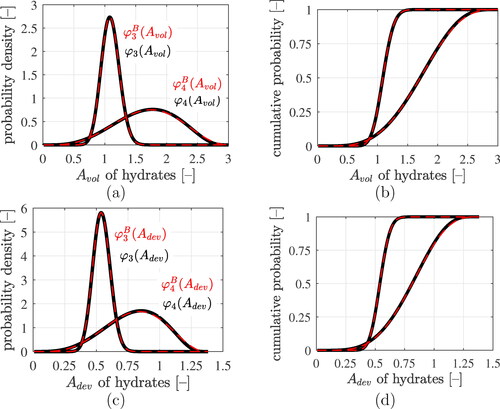54) , respectively, allows for producing parametric plots showing probability density over stress concentration tensor components, with the indentation modulus as the parameter. Normalizing the obtained parametric plots such that the area under the graphs becomes equal to 1, delivers probability density functions for the stress concentration tensor components, see Fig. 9. The probability densities of B_vol and B_dev of the LDCR hydrates are right-skewed functions. The corresponding results obtained for the HDCR hydrates, in turn, are reminiscent of Gaussian distributions.

Figure 9. Results of the lognormal microelasticity model (black graphs): statistical distributions of volumetric and deviatoric components of the stress concentration tensors of LDCR hydrates and of HDCR hydrates: (a) and (c) show probability density distributions, (b) and (d) cumulative distribution functions. The best fits of generalized beta-distributions to the statistical distributions are the red dashed graphs, see Eqs. (70)(70) $${\phi }_i^B(y)=\frac{{\left(\frac{y-a}{c-a}\right)}^{\alpha -1}{\left(\frac{c-y}{c-a}\right)}^{\beta -1}}{(c-a)\times B(\alpha ,\beta )},$$(70) and (71)(71) $$B(\alpha ,\beta )=\frac{\Gamma (\alpha )\Gamma (\beta )}{\Gamma (\alpha +\beta )},$$(71) as well as the Beta distributions parameters listed in Table 7.

The stress concentration tensor components averaged over each one of the two populations of hydrates are quantified based on the volume average rule for stress concentration tensors [26]: (66) $${\overline{B_{\mathit{vol}}}}_{,j}=\mathrm{ }\underset{0}{\overset{\infty }{\int }}{\phi }_j(M)B_{\mathit{vol},j}(M) \mathrm{d}M,\mathrm{\hspace{1em}}\mathrm{\hspace{1em}}j=3,4,$$(66) (67) $${\overline{B_{\mathit{dev}}}}_{,j}=\underset{0}{\overset{\infty }{\int }}{\phi }_j(M)B_{\mathit{dev},j}(M) \mathrm{d}M,\mathrm{\hspace{1em}}\mathrm{\hspace{1em}}j=3,4.$$(67) Inserting $B_{\mathit{vol},j}(M)$ and $B_{\mathit{dev},j}(M)$ according to Eqs. (53)(53) $$\begin{array}{c}{B}_{\mathit{vol},i}(M)=\frac{k_i(M)/k_{\mathit{bio}}}{1+\frac{S_{\mathit{vol}}(k_i(M)-k_{\mathit{bio}})}{k_{\mathit{bio}}}}\{\sum _{i=1}^2\frac{f_i}{1+\frac{S_{\mathit{vol}}(k_i-k_{\mathit{bio}})}{k_{\mathit{bio}}}}\\ +\sum _{i=3}^4{f}_i\mathrm{ }\underset{0}{\overset{\infty }{\int }}\frac{{\phi }_i(M)}{1+\frac{S_{\mathit{vol}}(k_i(M)-k_{\mathit{bio}})}{k_{\mathit{bio}}}} \mathrm{d}M{\}}^{-1},\end{array}$$(53) and (54)(54) $$\begin{array}{c}{B}_{\mathit{dev},i}(M)=\frac{g_i(M)/g_{\mathit{bio}}}{1+\frac{S_{\mathit{dev}}(g_i(M)-g_{\mathit{bio}})}{g_{\mathit{bio}}}}\{\sum _{i=1}^2\frac{f_i}{1+\frac{S_{\mathit{dev}}(g_i-g_{\mathit{bio}})}{g_{\mathit{bio}}}}\\ +\sum _{i=3}^4{f}_i\underset{0}{\overset{\infty }{\int }}\mathrm{ }\frac{{\phi }_i(M)}{1+\frac{S_{\mathit{dev}}(g_i(M)-g_{\mathit{bio}})}{g_{\mathit{bio}}}} \mathrm{d}M+\frac{4\pi \omega }{3}{T}_{\mathit{dev}}{\}}^{-1},\end{array}$$(54) , respectively, into Eqs. (66)(66) $${\overline{B_{\mathit{vol}}}}_{,j}=\mathrm{ }\underset{0}{\overset{\infty }{\int }}{\phi }_j(M)B_{\mathit{vol},j}(M) \mathrm{d}M,\mathrm{\hspace{1em}}\mathrm{\hspace{1em}}j=3,4,$$(66) and (67)(67) $${\overline{B_{\mathit{dev}}}}_{,j}=\underset{0}{\overset{\infty }{\int }}{\phi }_j(M)B_{\mathit{dev},j}(M) \mathrm{d}M,\mathrm{\hspace{1em}}\mathrm{\hspace{1em}}j=3,4.$$(67) yields (68) $$\begin{array}{c}\overline{B_{\mathit{vol},j}}=\frac{1}{k_{\mathit{bio}}}\underset{0}{\overset{\infty }{\int }}\frac{{\phi }_j(M)k_j(M)}{1+\frac{S_{\mathit{vol}}(k_j(M)-k_{\mathit{bio}})}{k_{\mathit{bio}}}} \mathrm{d}M\\ \times {\{\sum _{i=1}^2\frac{f_i}{1+\frac{S_{\mathit{vol}}(k_i-k_{\mathit{bio}})}{k_{\mathit{bio}}}}+\sum _{i=3}^4{f}_i\mathrm{ }\underset{0}{\overset{\infty }{\int }}\frac{{\phi }_i(M)}{1+\frac{S_{\mathit{vol}}(k_i(M)-k_{\mathit{bio}})}{k_{\mathit{bio}}}} \mathrm{d}M\}}^{-1},\end{array}$$(68) (69) $$\begin{array}{c}\overline{B_{\mathit{dev},j}}=\frac{1}{g_{\mathit{bio}}}\underset{0}{\overset{\infty }{\int }}\frac{{\phi }_j(M)g_j(M)}{1+\frac{S_{\mathit{dev}}(g_j(M)-g_{\mathit{bio}})}{g_{\mathit{bio}}}} \mathrm{d}M\\ \times \{\sum _{i=1}^2\frac{f_i}{1+\frac{S_{\mathit{dev}}(g_i-g_{\mathit{bio}})}{g_{\mathit{bio}}}}+\sum _{i=3}^4{f}_i\mathrm{ }\underset{0}{\overset{\infty }{\int }}\frac{{\phi }_i(M)}{1+\frac{S_{\mathit{dev}}(g_i(M)-g_{\mathit{bio}})}{g_{\mathit{bio}}}} \mathrm{d}M+\frac{4\pi \omega }{3}{T}_{\mathit{dev}}{\}}^{-1}.\end{array}$$(69) Evaluation of the stress concentration tensor components B_vol and B_dev of zirconia and clinker according to Eqs. (51)(51) $$\begin{array}{c}{B}_{\mathit{vol},i}=\frac{k_i/k_{\mathit{bio}}}{1+\frac{S_{\mathit{vol}}(k_i-k_{\mathit{bio}})}{k_{\mathit{bio}}}}\{\sum _{i=1}^2\frac{f_i}{1+\frac{S_{\mathit{vol}}(k_i-k_{\mathit{bio}})}{k_{\mathit{bio}}}}\\ +\sum _{i=3}^4{f}_i\mathrm{ }\underset{0}{\overset{\infty }{\int }}\frac{{\phi }_i(M)}{1+\frac{S_{\mathit{vol}}(k_i(M)-k_{\mathit{bio}})}{k_{\mathit{bio}}}} \mathrm{d}M{\}}^{-1},\end{array}$$(51) and (52)(52) $$\begin{array}{c}{B}_{\mathit{dev},i}=\frac{g_i/g_{\mathit{bio}}}{1+\frac{S_{\mathit{dev}}(g_i-g_{\mathit{bio}})}{g_{\mathit{bio}}}}\{\sum _{i=1}^2\frac{f_i}{1+\frac{S_{\mathit{dev}}(g_i-g_{\mathit{bio}})}{g_{\mathit{bio}}}}\\ +\sum _{i=3}^4{f}_i\underset{0}{\overset{\infty }{\int }}\mathrm{ }\frac{{\phi }_i(M)}{1+\frac{S_{\mathit{dev}}(g_i(M)-g_{\mathit{bio}})}{g_{\mathit{bio}}}} \mathrm{d}M+\frac{4\pi \omega }{3}{T}_{\mathit{dev}}{\}}^{-1}.\end{array}$$(52) , as well as the average stress concentration tensor components $\overline{B_{\mathit{vol}}}$ and $\overline{B_{\mathit{dev}}}$ of HDCR and LDCR hydrates according to Eqs. (68)(68) $$\begin{array}{c}\overline{B_{\mathit{vol},j}}=\frac{1}{k_{\mathit{bio}}}\underset{0}{\overset{\infty }{\int }}\frac{{\phi }_j(M)k_j(M)}{1+\frac{S_{\mathit{vol}}(k_j(M)-k_{\mathit{bio}})}{k_{\mathit{bio}}}} \mathrm{d}M\\ \times {\{\sum _{i=1}^2\frac{f_i}{1+\frac{S_{\mathit{vol}}(k_i-k_{\mathit{bio}})}{k_{\mathit{bio}}}}+\sum _{i=3}^4{f}_i\mathrm{ }\underset{0}{\overset{\infty }{\int }}\frac{{\phi }_i(M)}{1+\frac{S_{\mathit{vol}}(k_i(M)-k_{\mathit{bio}})}{k_{\mathit{bio}}}} \mathrm{d}M\}}^{-1},\end{array}$$(68) and (69)(69) $$\begin{array}{c}\overline{B_{\mathit{dev},j}}=\frac{1}{g_{\mathit{bio}}}\underset{0}{\overset{\infty }{\int }}\frac{{\phi }_j(M)g_j(M)}{1+\frac{S_{\mathit{dev}}(g_j(M)-g_{\mathit{bio}})}{g_{\mathit{bio}}}} \mathrm{d}M\\ \times \{\sum _{i=1}^2\frac{f_i}{1+\frac{S_{\mathit{dev}}(g_i-g_{\mathit{bio}})}{g_{\mathit{bio}}}}+\sum _{i=3}^4{f}_i\mathrm{ }\underset{0}{\overset{\infty }{\int }}\frac{{\phi }_i(M)}{1+\frac{S_{\mathit{dev}}(g_i(M)-g_{\mathit{bio}})}{g_{\mathit{bio}}}} \mathrm{d}M+\frac{4\pi \omega }{3}{T}_{\mathit{dev}}{\}}^{-1}.\end{array}$$(69) , yields numerical values listed in Table 5. These values quantify the expected trend that stresses experienced by the material constituents decrease with decreasing stiffness.

Table 5. Results of the lognormal microelasticity model: (population-averaged) stress concentration tensors components of the four types of solid constituents of Biodentine.

Constituent of Biodentine	(Average) stress concentration tensor components		Source
zirconia	$B_{\mathit{vol},1}=1.3419$	$B_{\mathit{dev},1}=1.3152$	Eqs. (49)(49) $$B_{\mathit{vol},i}=\frac{k_i}{k_{\mathit{bio}}}{A}_{\mathit{vol},i},$$(49) and (50)(50) $$B_{\mathit{dev},i}=\frac{g_i}{g_{\mathit{bio}}}{A}_{\mathit{dev},i},$$(50)
clinker	$B_{\mathit{vol},2}=1.2828$	$B_{\mathit{dev},2}=1.2188$	Eqs. (49)(49) $$B_{\mathit{vol},i}=\frac{k_i}{k_{\mathit{bio}}}{A}_{\mathit{vol},i},$$(49) and (50)(50) $$B_{\mathit{dev},i}=\frac{g_i}{g_{\mathit{bio}}}{A}_{\mathit{dev},i},$$(50)
HDCR hydrates	${\overline{B_{\mathit{vol}}}}_{,3}=0.9730$	${\overline{B_{\mathit{dev}}}}_{,3}=0.9830$	Eqs. (68)(68) $$\begin{array}{c}\overline{B_{\mathit{vol},j}}=\frac{1}{k_{\mathit{bio}}}\underset{0}{\overset{\infty }{\int }}\frac{{\phi }_j(M)k_j(M)}{1+\frac{S_{\mathit{vol}}(k_j(M)-k_{\mathit{bio}})}{k_{\mathit{bio}}}} \mathrm{d}M\\ \times {\{\sum _{i=1}^2\frac{f_i}{1+\frac{S_{\mathit{vol}}(k_i-k_{\mathit{bio}})}{k_{\mathit{bio}}}}+\sum _{i=3}^4{f}_i\mathrm{ }\underset{0}{\overset{\infty }{\int }}\frac{{\phi }_i(M)}{1+\frac{S_{\mathit{vol}}(k_i(M)-k_{\mathit{bio}})}{k_{\mathit{bio}}}} \mathrm{d}M\}}^{-1},\end{array}$$(68) and (69)(69) $$\begin{array}{c}\overline{B_{\mathit{dev},j}}=\frac{1}{g_{\mathit{bio}}}\underset{0}{\overset{\infty }{\int }}\frac{{\phi }_j(M)g_j(M)}{1+\frac{S_{\mathit{dev}}(g_j(M)-g_{\mathit{bio}})}{g_{\mathit{bio}}}} \mathrm{d}M\\ \times \{\sum _{i=1}^2\frac{f_i}{1+\frac{S_{\mathit{dev}}(g_i-g_{\mathit{bio}})}{g_{\mathit{bio}}}}+\sum _{i=3}^4{f}_i\mathrm{ }\underset{0}{\overset{\infty }{\int }}\frac{{\phi }_i(M)}{1+\frac{S_{\mathit{dev}}(g_i(M)-g_{\mathit{bio}})}{g_{\mathit{bio}}}} \mathrm{d}M+\frac{4\pi \omega }{3}{T}_{\mathit{dev}}{\}}^{-1}.\end{array}$$(69)
LDCR hydrates	${\overline{B_{\mathit{vol}}}}_{,4}=0.8430$	${\overline{B_{\mathit{dev}}}}_{,4}=0.8476$	Eqs. (68)(68) $$\begin{array}{c}\overline{B_{\mathit{vol},j}}=\frac{1}{k_{\mathit{bio}}}\underset{0}{\overset{\infty }{\int }}\frac{{\phi }_j(M)k_j(M)}{1+\frac{S_{\mathit{vol}}(k_j(M)-k_{\mathit{bio}})}{k_{\mathit{bio}}}} \mathrm{d}M\\ \times {\{\sum _{i=1}^2\frac{f_i}{1+\frac{S_{\mathit{vol}}(k_i-k_{\mathit{bio}})}{k_{\mathit{bio}}}}+\sum _{i=3}^4{f}_i\mathrm{ }\underset{0}{\overset{\infty }{\int }}\frac{{\phi }_i(M)}{1+\frac{S_{\mathit{vol}}(k_i(M)-k_{\mathit{bio}})}{k_{\mathit{bio}}}} \mathrm{d}M\}}^{-1},\end{array}$$(68) and (69)(69) $$\begin{array}{c}\overline{B_{\mathit{dev},j}}=\frac{1}{g_{\mathit{bio}}}\underset{0}{\overset{\infty }{\int }}\frac{{\phi }_j(M)g_j(M)}{1+\frac{S_{\mathit{dev}}(g_j(M)-g_{\mathit{bio}})}{g_{\mathit{bio}}}} \mathrm{d}M\\ \times \{\sum _{i=1}^2\frac{f_i}{1+\frac{S_{\mathit{dev}}(g_i-g_{\mathit{bio}})}{g_{\mathit{bio}}}}+\sum _{i=3}^4{f}_i\mathrm{ }\underset{0}{\overset{\infty }{\int }}\frac{{\phi }_i(M)}{1+\frac{S_{\mathit{dev}}(g_i(M)-g_{\mathit{bio}})}{g_{\mathit{bio}}}} \mathrm{d}M+\frac{4\pi \omega }{3}{T}_{\mathit{dev}}{\}}^{-1}.\end{array}$$(69)

3.3. Reproducing the distributions of strain and stress concentration tensor components based on generalized beta-distributions

Probability density functions ${\phi }_i(A_{\mathit{vol}}),{\phi }_i(A_{\mathit{dev}}),{\phi }_i(B_{\mathit{vol}})$ and ${\phi }_i(B_{\mathit{dev}})$ of both populations of hydrates (i = 3, 4) can be approximated by means of generalized beta-distributions: (70) $${\phi }_i^B(y)=\frac{{\left(\frac{y-a}{c-a}\right)}^{\alpha -1}{\left(\frac{c-y}{c-a}\right)}^{\beta -1}}{(c-a)\times B(\alpha ,\beta )},$$(70) where y denotes the statistical variable ranging in the interval $[a ; c],$ and $B(\alpha ,\beta )$ denotes the beta-distribution evaluated for parameters α and β: (71) $$B(\alpha ,\beta )=\frac{\Gamma (\alpha )\Gamma (\beta )}{\Gamma (\alpha +\beta )},$$(71) where Γ denotes the gamma function [34, 35].

Optimal α and β parameters are identified by means of the “Nonlinear Least Squares” method of MATLAB, see Tables 6 and 7 for the results. The lowest coefficient of determination, R², amounts to 0.9992 and is obtained for the deviatoric components of strain as well as stress concentration tensors of LDCR hydrates, see Tables 6 and 7 as well as Figs. 8 and 9. Notably, the α parameters found for the strain concentration tensor components are identical to the β parameters of the corresponding stress concentration tensor components, and vice versa, because strain and stress concentration tensor components are linearly related via Eqs. (49)(49) $$B_{\mathit{vol},i}=\frac{k_i}{k_{\mathit{bio}}}{A}_{\mathit{vol},i},$$(49) and (50)(50) $$B_{\mathit{dev},i}=\frac{g_i}{g_{\mathit{bio}}}{A}_{\mathit{dev},i},$$(50) .

Table 6. Optimal parameters of generalized beta-distributions, see Eqs. (70)(70) $${\phi }_i^B(y)=\frac{{\left(\frac{y-a}{c-a}\right)}^{\alpha -1}{\left(\frac{c-y}{c-a}\right)}^{\beta -1}}{(c-a)\times B(\alpha ,\beta )},$$(70) and (71)(71) $$B(\alpha ,\beta )=\frac{\Gamma (\alpha )\Gamma (\beta )}{\Gamma (\alpha +\beta )},$$(71) , approximating the distributions of the volumetric and deviatoric strain concentration tensor components of both populations of hydrates, see also the dashed red lines in Fig. 8; R² denotes coefficients of determination.

	HDCR hydrates		LDCR hydrates
Parameter	${\phi }_3(A_{\mathit{vol}})$	${\phi }_3(A_{\mathit{dev}})$	${\phi }_4(A_{\mathit{vol}})$	${\phi }_4(A_{\mathit{dev}})$
a	0.0136	0.0071	0.0136	0.0071
c	3.0427	1.3816	3.0427	1.3816
α	35.2406	37.0711	4.6942	4.9316
β	63.8869	58.4258	3.7593	3.5650
R^2	1.0000	1.0000	0.9995	0.9992

Table 7. Optimal parameters of generalized beta-distributions, see Eqs. (70)(70) $${\phi }_i^B(y)=\frac{{\left(\frac{y-a}{c-a}\right)}^{\alpha -1}{\left(\frac{c-y}{c-a}\right)}^{\beta -1}}{(c-a)\times B(\alpha ,\beta )},$$(70) and (71)(71) $$B(\alpha ,\beta )=\frac{\Gamma (\alpha )\Gamma (\beta )}{\Gamma (\alpha +\beta )},$$(71) , approximating the distributions of the volumetric and deviatoric stress concentration tensor components of both populations of hydrates, see also the dashed red lines in Fig. 9; R² denotes coefficients of determination.

	HDCR hydrates		LDCR hydrates
Parameter	${\phi }_3(B_{\mathit{vol}})$	${\phi }_3(B_{\mathit{dev}})$	${\phi }_4(B_{\mathit{vol}})$	${\phi }_4(B_{\mathit{dev}})$
a	$4.3\times {10}^{-5}$	$3.9\times {10}^{-5}$	$4.3\times {10}^{-5}$	$3.9\times {10}^{-5}$
c	1.4829	1.5768	1.4829	1.5768
α	63.8869	58.4258	3.7593	3.5650
β	35.2406	37.0711	4.6942	4.9316
R^2	1.0000	1.0000	0.9995	0.9992

3.4. Contribution of the microcracks to the stress and strain average rules

Closed microcracks do neither contribute to the stress average rule nor to the volumetric part of the strain average rule. Still, they contribute significantly to the deviatoric deformation of Biodentine, as will be shown next.

Insertion of Eq. (12)(12) $${\mathit{\sigma }}_i={\mathbb{B}}_i:\mathbf{\Sigma },\mathrm{\hspace{1em}}\mathrm{\hspace{1em}}i=1,2,\dots ,N.$$(12) , into Eq. (5)(5) $${\mathit{\sigma }}_i=\frac{1}{V_i}\underset{V_i}{\overset{}{\int }}\mathit{\sigma }(\underset{¯}{x}) \mathrm{d}V,\mathrm{\hspace{1em}}\mathrm{\hspace{1em}}i=1,2,\dots ,N.$$(5) yields the stress average rule expressed in terms of stress concentration tensors: (72) $$\sum _{i=1}^N{f}_i{\mathbb{B}}_i=\mathbb{I}.$$(72) Closed microcracks transfer finite stresses across their microcrack planes. Therefore, their stress concentration tensor components are finite. The volume fraction of closed microcracks is equal to zero. Therefore, closed microcracks have a vanishing contribution to Eq. (72)(72) $$\sum _{i=1}^N{f}_i{\mathbb{B}}_i=\mathbb{I}.$$(72) . Subdividing this equation into volumetric and deviatoric parts, and consideration of volume fractions according to Table 2 as well as (hydrate population-averaged) stress concentration tensor components according to Table 5, yields (73) $$f_1{B}_{\mathit{vol},1}+f_2{B}_{\mathit{vol},2}+f_3{\overline{B_{\mathit{vol}}}}_{,3}+f_4{\overline{B_{\mathit{vol}}}}_{,4}=1,$$(73) (74) $$f_1{B}_{\mathit{dev},1}+f_2{B}_{\mathit{dev},2}+f_3{\overline{B_{\mathit{dev}}}}_{,3}+f_4{\overline{B_{\mathit{dev}}}}_{,4}=1.$$(74) Similarly, insertion Eq. (9)(9) $${\mathit{\epsilon }}_i={\mathbb{A}}_i:\mathbf{E},\mathrm{\hspace{1em}}\mathrm{\hspace{1em}}i=1,2,\dots ,N.$$(9) into Eq. (4)(4) $${\mathit{\epsilon }}_i=\frac{1}{V_i}\underset{V_i}{\overset{}{\int }}\mathit{\epsilon }(\underset{¯}{x}) \mathrm{d}V,\mathrm{\hspace{1em}}\mathrm{\hspace{1em}}i=1,2,\dots ,N,$$(4) yields the strain average rule expressed in terms of strain concentration tensors: (75) $$\sum _{i=1}^N{f}_i{\mathbb{A}}_i=\mathbb{I}.$$(75) Because closed microcracks occupy a vanishing volume and because they remain closed also under macroscopic loading, they have a vanishing contribution to the volumetric part of Eq. (75)(75) $$\sum _{i=1}^N{f}_i{\mathbb{A}}_i=\mathbb{I}.$$(75) : (76) $$f_1{A}_{\mathit{vol},1}+f_2{A}_{\mathit{vol},2}+f_3{\overline{A_{\mathit{vol}}}}_{,3}+f_4{\overline{A_{\mathit{vol}}}}_{,4}=1,$$(76) where volume fractions according to Table 2 and (hydrate population-averaged) strain concentration tensor components according to Table 4 were used. However, the same approach applied to the deviatoric part of Eq. (75)(75) $$\sum _{i=1}^N{f}_i{\mathbb{A}}_i=\mathbb{I}.$$(75) yields: (77) $$f_1{A}_{\mathit{dev},1}+f_2{A}_{\mathit{dev},2}+f_3{\overline{A_{\mathit{dev}}}}_{,3}+f_4{\overline{A_{\mathit{dev}}}}_{,4}=0.5100\ne 1.$$(77) Eq. (77)(77) $$f_1{A}_{\mathit{dev},1}+f_2{A}_{\mathit{dev},2}+f_3{\overline{A_{\mathit{dev}}}}_{,3}+f_4{\overline{A_{\mathit{dev}}}}_{,4}=0.5100\ne 1.$$(77) underlines that closed cracks contribute to the deviatoric compliance of the homogenized material.

In order to quantify the contribution of the microcracks missing in Eq. (77)(77) $$f_1{A}_{\mathit{dev},1}+f_2{A}_{\mathit{dev},2}+f_3{\overline{A_{\mathit{dev}}}}_{,3}+f_4{\overline{A_{\mathit{dev}}}}_{,4}=0.5100\ne 1.$$(77) , their population-averaged (= orientation-averaged) strain concentration tensor is introduced, while the cracks are still considered as thin but slightly open oblate spheroids: (78) $$\begin{array}{c}{\overline{\mathbb{A}}}_5=\underset{0}{\overset{\pi }{\int }}\underset{0}{\overset{2\pi }{\int }}{[\mathbb{I}+{\mathbb{P}}_{\mathit{obl}}(\psi ,\vartheta ):({\mathbb{C}}_5-{\mathbb{C}}_{\mathit{bio}})]}^{-1} \frac{\hspace{0.17em}\text{sin}\hspace{0.17em}\vartheta }{4\pi } d\psi d\vartheta \\ :\{\sum _{j=1}^2{f}_j{[\mathbb{I}+{\mathbb{P}}_{\mathit{sph}}:({\mathbb{C}}_j-{\mathbb{C}}_{\mathit{bio}})]}^{-1}\\ +\sum _{j=3}^4{f}_j\underset{0}{\overset{\infty }{\int }}{\phi }_j(M){[\mathbb{I}+{\mathbb{P}}_{\mathit{sph}}:({\mathbb{C}}_j(M)-{\mathbb{C}}_{\mathit{bio}})]}^{-1} \mathrm{d}M\\ +f_5\mathrm{ }\underset{0}{\overset{\pi }{\int }}\underset{0}{\overset{2\pi }{\int }}{[\mathbb{I}+{\mathbb{P}}_{\mathit{obl}}(\psi ,\vartheta ):({\mathbb{C}}_5-{\mathbb{C}}_{\mathit{bio}})]}^{-1} \frac{\hspace{0.17em}\text{sin}\hspace{0.17em}\vartheta }{4\pi } d\psi d\vartheta {\}}^{-1}.\end{array}$$(78) The transition to circular slit cracks refers to the limit case that the aspect ratio of the microcracks approaches zero: $X\to 0.$ In this limit case, the deviatoric component of ${\overline{\mathbb{A}}}_5$ approaches infinity [29], while the volume fraction of the population of microcracks, f₅, approaches zero, such that the product of f₅ and ${\overline{\mathbb{A}}}_5$ remains finite: (79) $$\begin{array}{c}\underset{X\to 0}{\lim }{f}_5{\overline{\mathbb{A}}}_5=\frac{4\pi \omega }{3}{T}_{\mathit{dev}}\{\sum _{i=1}^2\frac{f_i}{1+\frac{S_{\mathit{dev}}(g_i-g_{\mathit{bio}})}{g_{\mathit{bio}}}}\\ +\sum _{i=3}^4{f}_i\mathrm{ }\underset{0}{\overset{\infty }{\int }}\frac{{\phi }_i(M)}{1+\frac{S_{\mathit{dev}}(g_i(M)-g_{\mathit{bio}})}{g_{\mathit{bio}}}} \mathrm{d}M+\frac{4\pi \omega }{3}{T}_{\mathit{dev}}{\}}^{-1}{\mathbb{I}}^{\mathit{dev}}.\end{array}$$(79) Evaluation of Eq. (79)(79) $$\begin{array}{c}\underset{X\to 0}{\lim }{f}_5{\overline{\mathbb{A}}}_5=\frac{4\pi \omega }{3}{T}_{\mathit{dev}}\{\sum _{i=1}^2\frac{f_i}{1+\frac{S_{\mathit{dev}}(g_i-g_{\mathit{bio}})}{g_{\mathit{bio}}}}\\ +\sum _{i=3}^4{f}_i\mathrm{ }\underset{0}{\overset{\infty }{\int }}\frac{{\phi }_i(M)}{1+\frac{S_{\mathit{dev}}(g_i(M)-g_{\mathit{bio}})}{g_{\mathit{bio}}}} \mathrm{d}M+\frac{4\pi \omega }{3}{T}_{\mathit{dev}}{\}}^{-1}{\mathbb{I}}^{\mathit{dev}}.\end{array}$$(79) based on k_bio = 38.4 GPa, g_bio = 14.1 GPa, T_dev from Eq. (35)(35) $$T_{\mathit{dev}}=\frac{8(3k_{\mathit{bio}}+4g_{\mathit{bio}})}{15\pi (3k_{\mathit{bio}}+2g_{\mathit{bio}})}.$$(35) , S_dev from Eq. (40)(40) $$S_{\mathit{dev}}=\frac{6(k_{\mathit{bio}}+2g_{\mathit{bio}})}{5(3k_{\mathit{bio}}+4g_{\mathit{bio}})}.$$(40) , together with ω from Eq. (60)(60) $$\omega =0.7802,$$(60) , and volume fractions from Table 2 yields, under consideration of Eqs. (B.7)(B.7) $$\underset{0}{\overset{\infty }{\int }}\frac{{\phi }_3(M)}{1+\frac{S_{\mathit{dev}}(g_3(M)-g_{\mathit{bio}})}{g_{\mathit{bio}}}} \mathrm{d}M=0.71090769,$$(B.7) and (B.8)(B.8) $$\underset{0}{\overset{\infty }{\int }}\frac{{\phi }_4(M)}{1+\frac{S_{\mathit{dev}}(g_4(M)-g_{\mathit{bio}})}{g_{\mathit{bio}}}} \mathrm{d}M=0.87075413.$$(B.8) : (80) $$\underset{X\to 0}{\lim }{f}_5{\overline{\mathbb{A}}}_5=f_5{\overline{A_{\mathit{dev}}}}_{,5}{\mathbb{I}}^{\mathit{dev}}=0.4899{\mathbb{I}}^{\mathit{dev}}.$$(80) Adding $f_5{\overline{A_{\mathit{dev}}}}_{,5}$ according to Eq. (80)(80) $$\underset{X\to 0}{\lim }{f}_5{\overline{\mathbb{A}}}_5=f_5{\overline{A_{\mathit{dev}}}}_{,5}{\mathbb{I}}^{\mathit{dev}}=0.4899{\mathbb{I}}^{\mathit{dev}}.$$(80) to Eq. (77)(77) $$f_1{A}_{\mathit{dev},1}+f_2{A}_{\mathit{dev},2}+f_3{\overline{A_{\mathit{dev}}}}_{,3}+f_4{\overline{A_{\mathit{dev}}}}_{,4}=0.5100\ne 1.$$(77) yields (81) $$f_1{A}_{\mathit{dev},1}+f_2{A}_{\mathit{dev},2}+f_3{\overline{A_{\mathit{dev}}}}_{,3}+f_4{\overline{A_{\mathit{dev}}}}_{,4}+f_5{\overline{A_{\mathit{dev}}}}_{,5}=1.$$(81) Eqs. (80)(80) $$\underset{X\to 0}{\lim }{f}_5{\overline{\mathbb{A}}}_5=f_5{\overline{A_{\mathit{dev}}}}_{,5}{\mathbb{I}}^{\mathit{dev}}=0.4899{\mathbb{I}}^{\mathit{dev}}.$$(80) and (81)(81) $$f_1{A}_{\mathit{dev},1}+f_2{A}_{\mathit{dev},2}+f_3{\overline{A_{\mathit{dev}}}}_{,3}+f_4{\overline{A_{\mathit{dev}}}}_{,4}+f_5{\overline{A_{\mathit{dev}}}}_{,5}=1.$$(81) underline that almost 50% of the deviatoric deformation of Biodentine results from shear-dislocations of closed microcracks.

4. Piecewise uniform microelasticity models

The developed lognormal microelasticity model accounts for stiffness distributions of hydrates, as characterized in a grid nanoindentation testing campaign. Standardly used multiscale models for cementitious materials, in turn, assign characteristic stiffness constants to a small number of considered hydrate phases, typically two. This provides the motivation to identify characteristic stiffness constants of HDCR hydrates and LDCR hydrates such that a piecewise uniform microelasticity model, based on four solid phases and infinitely many crack phases, reproduces the same homogenized stiffness as the lognormal microelasticity model described above. In the piecewise uniform microelasticity model, Biodentine is represented as a composite with polycrystalline microstructure in which four spherical solid phases (zirconia, clinker, HDCR hydrates, and LDCR hydrates) and infinitely many crack phases (which are isotropically oriented in space) directly interact with each other, see Fig. 10.

Figure 10. Micromechanical representation of Biodentine (“material organogram”): the two-dimensional sketch shows qualitative properties of a three-dimensional representative volume element of the piecewise uniform microelasticity models which account for characteristic stiffness constants of two populations of hydrates.

The stiffness constants of zirconia and clinker, the volume fractions of the four solid phases, and the crack density are the same as before, see Table 2 and Eq. (60)(60) $$\omega =0.7802,$$(60) . Denoting the characteristic bulk and shear moduli assigned to the two populations of hydrates as k₃ and k₄ as well as g₃ and g₄, respectively, the expressions for the homogenized bulk and shear moduli according to Eqs. (41)(41) $$\begin{array}{c}{k}_{\mathit{bio}}=\{\sum _{i=1}^2\frac{f_i{k}_i}{1+\frac{S_{\mathit{vol}}(k_i-k_{\mathit{bio}})}{k_{\mathit{bio}}}}+\sum _{i=3}^4{f}_i\underset{0}{\overset{\infty }{\int }}\frac{{\phi }_i(M)k_i(M)}{1+\frac{S_{\mathit{vol}}(k_i(M)-k_{\mathit{bio}})}{k_{\mathit{bio}}}} \mathrm{d}M\}\\ \times {\{\sum _{i=1}^2\frac{f_i}{1+\frac{S_{\mathit{vol}}(k_i-k_{\mathit{bio}})}{k_{\mathit{bio}}}}+\sum _{i=3}^4{f}_i\mathrm{ }\underset{0}{\overset{\infty }{\int }}\frac{{\phi }_i(M)}{1+\frac{S_{\mathit{vol}}(k_i(M)-k_{\mathit{bio}})}{k_{\mathit{bio}}}} \mathrm{d}M\}}^{-1},\end{array}$$(41) and (42)(42) $$\begin{array}{c}{g}_{\mathit{bio}}=\{\sum _{i=1}^2\frac{f_i{g}_i}{1+\frac{S_{\mathit{dev}}(g_i-g_{\mathit{bio}})}{g_{\mathit{bio}}}}+\sum _{i=3}^4{f}_i\underset{0}{\overset{\infty }{\int }}\frac{{\phi }_i(M)g_i(M)}{1+\frac{S_{\mathit{dev}}(g_i(M)-g_{\mathit{bio}})}{g_{\mathit{bio}}}} \mathrm{d}M\}\\ \times \{\sum _{i=1}^2\frac{f_i}{1+\frac{S_{\mathit{dev}}(g_i-g_{\mathit{bio}})}{g_{\mathit{bio}}}}+\sum _{i=3}^4{f}_i\underset{0}{\overset{\infty }{\int }}\frac{{\phi }_i(M)}{1+\frac{S_{\mathit{dev}}(g_i(M)-g_{\mathit{bio}})}{g_{\mathit{bio}}}} \mathrm{d}M\\ \hspace{1em}+\frac{4\pi \omega }{3}{T}_{\mathit{dev}}{\}}^{-1}.\end{array}$$(42) , those for the strain concentration tensor components according to Eqs. (44)–(47), and those for the stress concentration tensor components according to Eqs. (51)–(54) simplify to (82) $$k_{\mathit{bio}}=\left\{\sum _{i=1}^4\frac{f_i{k}_i}{1+\frac{S_{\mathit{vol}}(k_i-k_{\mathit{bio}})}{k_{\mathit{bio}}}}\right\}\times {\{\sum _{i=1}^4\frac{f_i}{1+\frac{S_{\mathit{vol}}(k_i-k_{\mathit{bio}})}{k_{\mathit{bio}}}}\}}^{-1},$$(82) (83) $$g_{\mathit{bio}}=\left\{\sum _{i=1}^4\frac{f_i{g}_i}{1+\frac{S_{\mathit{dev}}(g_i-g_{\mathit{bio}})}{g_{\mathit{bio}}}}\right\}\times {\{\sum _{i=1}^4\frac{f_i}{1+\frac{S_{\mathit{dev}}(g_i-g_{\mathit{bio}})}{g_{\mathit{bio}}}}+\frac{4\pi \omega }{3}{T}_{\mathit{dev}}\}}^{-1},$$(83) (84) $$A_{\mathit{vol},j}=\frac{1}{1+\frac{S_{\mathit{vol}}(k_j-k_{\mathit{bio}})}{k_{\mathit{bio}}}}\times {\left\{\sum _{i=1}^4\frac{f_i}{1+\frac{S_{\mathit{vol}}(k_i-k_{\mathit{bio}})}{k_{\mathit{bio}}}}\right\}}^{-1},$$(84) (85) $$A_{\mathit{dev},j}=\frac{1}{1+\frac{S_{\mathit{dev}}(g_j-g_{\mathit{bio}})}{g_{\mathit{bio}}}}\times {\{\sum _{i=1}^4\frac{f_i}{1+\frac{S_{\mathit{dev}}(g_i-g_{\mathit{bio}})}{g_{\mathit{bio}}}}+\frac{4\pi \omega }{3}{T}_{\mathit{dev}}\}}^{-1},$$(85) (86) $$B_{\mathit{vol},j}=\frac{k_j/k_{\mathit{bio}}}{1+\frac{S_{\mathit{vol}}(k_j-k_{\mathit{bio}})}{k_{\mathit{bio}}}}\times {\left\{\sum _{i=1}^4\frac{f_i}{1+\frac{S_{\mathit{vol}}(k_i-k_{\mathit{bio}})}{k_{\mathit{bio}}}}\right\}}^{-1},$$(86) (87) $$B_{\mathit{dev},j}=\frac{g_j/g_{\mathit{bio}}}{1+\frac{S_{\mathit{dev}}(g_j-g_{\mathit{bio}})}{g_{\mathit{bio}}}}\times {\{\sum _{i=1}^4\frac{f_i}{1+\frac{S_{\mathit{dev}}(g_i-g_{\mathit{bio}})}{g_{\mathit{bio}}}}+\frac{4\pi \omega }{3}{T}_{\mathit{dev}}\}}^{-1}.$$(87)

4.1. Averaging of hydrate strain and stress concentration tensors - piecewise uniform microelastic properties

Equivalent, piecewise uniform, bulk and shear moduli of LDCR and HDCR hydrates are determined from averaging over the strain and stress concentration tensor distributions of the two hydrate populations. Equivalent bulk moduli k₃ and k₄ are derived as follows. Equating $A_{\mathit{vol},j}$ according to Eq. (84)(84) $$A_{\mathit{vol},j}=\frac{1}{1+\frac{S_{\mathit{vol}}(k_j-k_{\mathit{bio}})}{k_{\mathit{bio}}}}\times {\left\{\sum _{i=1}^4\frac{f_i}{1+\frac{S_{\mathit{vol}}(k_i-k_{\mathit{bio}})}{k_{\mathit{bio}}}}\right\}}^{-1},$$(84) and ${\overline{A_{\mathit{vol}}}}_{,j}$ according to Eq. (64)(64) $$\begin{array}{c}\overline{A_{\mathit{vol},j}}=\underset{0}{\overset{\infty }{\int }}\frac{{\phi }_j(M)}{1+\frac{S_{\mathit{vol}}(k_j(M)-k_{\mathit{bio}})}{k_{\mathit{bio}}}} \mathrm{d}M\\ \times {\{\sum _{i=1}^2\frac{f_i}{1+\frac{S_{\mathit{vol}}(k_i-k_{\mathit{bio}})}{k_{\mathit{bio}}}}+\sum _{i=3}^4{f}_i\mathrm{ }\underset{0}{\overset{\infty }{\int }}\frac{{\phi }_i(M)}{1+\frac{S_{\mathit{vol}}(k_i(M)-k_{\mathit{bio}})}{k_{\mathit{bio}}}} \mathrm{d}M\}}^{-1},\end{array}$$(64) yields the conditions (88) $$\frac{1}{1+\frac{S_{\mathit{vol}}(k_j-k_{\mathit{bio}})}{k_{\mathit{bio}}}}=\mathrm{ }\underset{0}{\overset{\infty }{\int }}\frac{{\phi }_j(M)}{1+\frac{S_{\mathit{vol}}(k_j(M)-k_{\mathit{bio}})}{k_{\mathit{bio}}}} \mathrm{d}M,\mathrm{\hspace{1em}}\mathrm{\hspace{1em}}j=3,4.$$(88) Equating $B_{\mathit{vol},j}$ according to Eq. (86)(86) $$B_{\mathit{vol},j}=\frac{k_j/k_{\mathit{bio}}}{1+\frac{S_{\mathit{vol}}(k_j-k_{\mathit{bio}})}{k_{\mathit{bio}}}}\times {\left\{\sum _{i=1}^4\frac{f_i}{1+\frac{S_{\mathit{vol}}(k_i-k_{\mathit{bio}})}{k_{\mathit{bio}}}}\right\}}^{-1},$$(86) and ${\overline{B_{\mathit{vol}}}}_{,j}$ according to Eq. (68)(68) $$\begin{array}{c}\overline{B_{\mathit{vol},j}}=\frac{1}{k_{\mathit{bio}}}\underset{0}{\overset{\infty }{\int }}\frac{{\phi }_j(M)k_j(M)}{1+\frac{S_{\mathit{vol}}(k_j(M)-k_{\mathit{bio}})}{k_{\mathit{bio}}}} \mathrm{d}M\\ \times {\{\sum _{i=1}^2\frac{f_i}{1+\frac{S_{\mathit{vol}}(k_i-k_{\mathit{bio}})}{k_{\mathit{bio}}}}+\sum _{i=3}^4{f}_i\mathrm{ }\underset{0}{\overset{\infty }{\int }}\frac{{\phi }_i(M)}{1+\frac{S_{\mathit{vol}}(k_i(M)-k_{\mathit{bio}})}{k_{\mathit{bio}}}} \mathrm{d}M\}}^{-1},\end{array}$$(68) yields the conditions (89) $$\frac{k_j}{1+\frac{S_{\mathit{vol}}(k_j-k_{\mathit{bio}})}{k_{\mathit{bio}}}}=\underset{0}{\overset{\infty }{\int }}\frac{{\phi }_j(M)k_j(M)}{1+\frac{S_{\mathit{vol}}(k_j(M)-k_{\mathit{bio}})}{k_{\mathit{bio}}}} \mathrm{d}M,\mathrm{\hspace{1em}}\mathrm{\hspace{1em}}j=3,4.$$(89) Notably, the conditions (88)(88) $$\frac{1}{1+\frac{S_{\mathit{vol}}(k_j-k_{\mathit{bio}})}{k_{\mathit{bio}}}}=\mathrm{ }\underset{0}{\overset{\infty }{\int }}\frac{{\phi }_j(M)}{1+\frac{S_{\mathit{vol}}(k_j(M)-k_{\mathit{bio}})}{k_{\mathit{bio}}}} \mathrm{d}M,\mathrm{\hspace{1em}}\mathrm{\hspace{1em}}j=3,4.$$(88) and (89)(89) $$\frac{k_j}{1+\frac{S_{\mathit{vol}}(k_j-k_{\mathit{bio}})}{k_{\mathit{bio}}}}=\underset{0}{\overset{\infty }{\int }}\frac{{\phi }_j(M)k_j(M)}{1+\frac{S_{\mathit{vol}}(k_j(M)-k_{\mathit{bio}})}{k_{\mathit{bio}}}} \mathrm{d}M,\mathrm{\hspace{1em}}\mathrm{\hspace{1em}}j=3,4.$$(89) also imply the equality of k_bio according to Eqs. (41)(41) $$\begin{array}{c}{k}_{\mathit{bio}}=\{\sum _{i=1}^2\frac{f_i{k}_i}{1+\frac{S_{\mathit{vol}}(k_i-k_{\mathit{bio}})}{k_{\mathit{bio}}}}+\sum _{i=3}^4{f}_i\underset{0}{\overset{\infty }{\int }}\frac{{\phi }_i(M)k_i(M)}{1+\frac{S_{\mathit{vol}}(k_i(M)-k_{\mathit{bio}})}{k_{\mathit{bio}}}} \mathrm{d}M\}\\ \times {\{\sum _{i=1}^2\frac{f_i}{1+\frac{S_{\mathit{vol}}(k_i-k_{\mathit{bio}})}{k_{\mathit{bio}}}}+\sum _{i=3}^4{f}_i\mathrm{ }\underset{0}{\overset{\infty }{\int }}\frac{{\phi }_i(M)}{1+\frac{S_{\mathit{vol}}(k_i(M)-k_{\mathit{bio}})}{k_{\mathit{bio}}}} \mathrm{d}M\}}^{-1},\end{array}$$(41) and (82)(82) $$k_{\mathit{bio}}=\left\{\sum _{i=1}^4\frac{f_i{k}_i}{1+\frac{S_{\mathit{vol}}(k_i-k_{\mathit{bio}})}{k_{\mathit{bio}}}}\right\}\times {\{\sum _{i=1}^4\frac{f_i}{1+\frac{S_{\mathit{vol}}(k_i-k_{\mathit{bio}})}{k_{\mathit{bio}}}}\}}^{-1},$$(82) . The equivalent bulk moduli k₃ and k₄ are obtained from dividing Eq. (89)(89) $$\frac{k_j}{1+\frac{S_{\mathit{vol}}(k_j-k_{\mathit{bio}})}{k_{\mathit{bio}}}}=\underset{0}{\overset{\infty }{\int }}\frac{{\phi }_j(M)k_j(M)}{1+\frac{S_{\mathit{vol}}(k_j(M)-k_{\mathit{bio}})}{k_{\mathit{bio}}}} \mathrm{d}M,\mathrm{\hspace{1em}}\mathrm{\hspace{1em}}j=3,4.$$(89) by Eq. (88)(88) $$\frac{1}{1+\frac{S_{\mathit{vol}}(k_j-k_{\mathit{bio}})}{k_{\mathit{bio}}}}=\mathrm{ }\underset{0}{\overset{\infty }{\int }}\frac{{\phi }_j(M)}{1+\frac{S_{\mathit{vol}}(k_j(M)-k_{\mathit{bio}})}{k_{\mathit{bio}}}} \mathrm{d}M,\mathrm{\hspace{1em}}\mathrm{\hspace{1em}}j=3,4.$$(88) as (90) $$k_j=\frac{\underset{0}{\overset{\infty }{\int }}\frac{{\phi }_j(M)k_j(M)}{1+\frac{S_{\mathit{vol}}(k_j(M)-k_{\mathit{bio}})}{k_{\mathit{bio}}}} \mathrm{d}M}{\underset{0}{\overset{\infty }{\int }}\frac{{\phi }_j(M)}{1+\frac{S_{\mathit{vol}}(k_j(M)-k_{\mathit{bio}})}{k_{\mathit{bio}}}} \mathrm{d}M},\mathrm{\hspace{1em}}\mathrm{\hspace{1em}}j=3,4.$$(90) Evaluating Eq. (90)(90) $$k_j=\frac{\underset{0}{\overset{\infty }{\int }}\frac{{\phi }_j(M)k_j(M)}{1+\frac{S_{\mathit{vol}}(k_j(M)-k_{\mathit{bio}})}{k_{\mathit{bio}}}} \mathrm{d}M}{\underset{0}{\overset{\infty }{\int }}\frac{{\phi }_j(M)}{1+\frac{S_{\mathit{vol}}(k_j(M)-k_{\mathit{bio}})}{k_{\mathit{bio}}}} \mathrm{d}M},\mathrm{\hspace{1em}}\mathrm{\hspace{1em}}j=3,4.$$(90) for j = 3 and for j = 4, respectively, yields under consideration of Eqs. (B.1)(B.1) $$\underset{0}{\overset{\infty }{\int }}\frac{{\phi }_3(M)k_3(M)}{1+\frac{S_{\mathit{vol}}(k_3(M)-k_{\mathit{bio}})}{k_{\mathit{bio}}}} \mathrm{d}M=37.36450836\text{GPa},$$(B.1) –(B.4)(B.4) $$\underset{0}{\overset{\infty }{\int }}\frac{{\phi }_4(M)}{1+\frac{S_{\mathit{vol}}(k_4(M)-k_{\mathit{bio}})}{k_{\mathit{bio}}}} \mathrm{d}M=1.32063926,$$(B.4) : (91) $$k_3=35.41\text{GPa},$$(91) (92) $$k_4=24.51\text{GPa}.$$(92) Equivalent shear moduli g₃ and g₄ are derived in an analogous way. Equating $A_{\mathit{dev},j}$ according to Eq. (85)(85) $$A_{\mathit{dev},j}=\frac{1}{1+\frac{S_{\mathit{dev}}(g_j-g_{\mathit{bio}})}{g_{\mathit{bio}}}}\times {\{\sum _{i=1}^4\frac{f_i}{1+\frac{S_{\mathit{dev}}(g_i-g_{\mathit{bio}})}{g_{\mathit{bio}}}}+\frac{4\pi \omega }{3}{T}_{\mathit{dev}}\}}^{-1},$$(85) and ${\overline{A_{\mathit{dev}}}}_{,j}$ according to Eq. (65)(65) $$\begin{array}{c}\overline{A_{\mathit{dev},j}}=\underset{0}{\overset{\infty }{\int }}\frac{{\phi }_j(M)}{1+\frac{S_{\mathit{dev}}(g_j(M)-g_{\mathit{bio}})}{g_{\mathit{bio}}}} \mathrm{d}M\\ \times \{\sum _{i=1}^2\frac{f_i}{1+\frac{S_{\mathit{dev}}(g_i-g_{\mathit{bio}})}{g_{\mathit{bio}}}}+\sum _{i=3}^4{f}_i\mathrm{ }\underset{0}{\overset{\infty }{\int }}\frac{{\phi }_i(M)}{1+\frac{S_{\mathit{dev}}(g_i(M)-g_{\mathit{bio}})}{g_{\mathit{bio}}}} \mathrm{d}M+\frac{4\pi \omega }{3}{T}_{\mathit{dev}}{\}}^{-1}.\end{array}$$(65) yields the conditions (93) $$\frac{1}{1+\frac{S_{\mathit{dev}}(g_j-g_{\mathit{bio}})}{g_{\mathit{bio}}}}=\mathrm{ }\underset{0}{\overset{\infty }{\int }}\frac{{\phi }_j(M)}{1+\frac{S_{\mathit{dev}}(g_j(M)-g_{\mathit{bio}})}{g_{\mathit{bio}}}} \mathrm{d}M,\mathrm{\hspace{1em}}\mathrm{\hspace{1em}}j=3,4.$$(93) Equating $B_{\mathit{dev},j}$ according to Eq. (87)(87) $$B_{\mathit{dev},j}=\frac{g_j/g_{\mathit{bio}}}{1+\frac{S_{\mathit{dev}}(g_j-g_{\mathit{bio}})}{g_{\mathit{bio}}}}\times {\{\sum _{i=1}^4\frac{f_i}{1+\frac{S_{\mathit{dev}}(g_i-g_{\mathit{bio}})}{g_{\mathit{bio}}}}+\frac{4\pi \omega }{3}{T}_{\mathit{dev}}\}}^{-1}.$$(87) and ${\overline{B_{\mathit{dev}}}}_{,j}$ according to Eq. (69)(69) $$\begin{array}{c}\overline{B_{\mathit{dev},j}}=\frac{1}{g_{\mathit{bio}}}\underset{0}{\overset{\infty }{\int }}\frac{{\phi }_j(M)g_j(M)}{1+\frac{S_{\mathit{dev}}(g_j(M)-g_{\mathit{bio}})}{g_{\mathit{bio}}}} \mathrm{d}M\\ \times \{\sum _{i=1}^2\frac{f_i}{1+\frac{S_{\mathit{dev}}(g_i-g_{\mathit{bio}})}{g_{\mathit{bio}}}}+\sum _{i=3}^4{f}_i\mathrm{ }\underset{0}{\overset{\infty }{\int }}\frac{{\phi }_i(M)}{1+\frac{S_{\mathit{dev}}(g_i(M)-g_{\mathit{bio}})}{g_{\mathit{bio}}}} \mathrm{d}M+\frac{4\pi \omega }{3}{T}_{\mathit{dev}}{\}}^{-1}.\end{array}$$(69) yields the conditions (94) $$\frac{g_j}{1+\frac{S_{\mathit{dev}}(g_j-g_{\mathit{bio}})}{g_{\mathit{bio}}}}=\mathrm{ }\underset{0}{\overset{\infty }{\int }}\frac{{\phi }_j(M)g_j(M)}{1+\frac{S_{\mathit{dev}}(g_j(M)-g_{\mathit{bio}})}{g_{\mathit{bio}}}} \mathrm{d}M,\mathrm{\hspace{1em}}\mathrm{\hspace{1em}}j=3,4.$$(94) Notably, the conditions (93)(93) $$\frac{1}{1+\frac{S_{\mathit{dev}}(g_j-g_{\mathit{bio}})}{g_{\mathit{bio}}}}=\mathrm{ }\underset{0}{\overset{\infty }{\int }}\frac{{\phi }_j(M)}{1+\frac{S_{\mathit{dev}}(g_j(M)-g_{\mathit{bio}})}{g_{\mathit{bio}}}} \mathrm{d}M,\mathrm{\hspace{1em}}\mathrm{\hspace{1em}}j=3,4.$$(93) and (94)(94) $$\frac{g_j}{1+\frac{S_{\mathit{dev}}(g_j-g_{\mathit{bio}})}{g_{\mathit{bio}}}}=\mathrm{ }\underset{0}{\overset{\infty }{\int }}\frac{{\phi }_j(M)g_j(M)}{1+\frac{S_{\mathit{dev}}(g_j(M)-g_{\mathit{bio}})}{g_{\mathit{bio}}}} \mathrm{d}M,\mathrm{\hspace{1em}}\mathrm{\hspace{1em}}j=3,4.$$(94) also imply the equality of g_bio according to Eqs. (42)(42) $$\begin{array}{c}{g}_{\mathit{bio}}=\{\sum _{i=1}^2\frac{f_i{g}_i}{1+\frac{S_{\mathit{dev}}(g_i-g_{\mathit{bio}})}{g_{\mathit{bio}}}}+\sum _{i=3}^4{f}_i\underset{0}{\overset{\infty }{\int }}\frac{{\phi }_i(M)g_i(M)}{1+\frac{S_{\mathit{dev}}(g_i(M)-g_{\mathit{bio}})}{g_{\mathit{bio}}}} \mathrm{d}M\}\\ \times \{\sum _{i=1}^2\frac{f_i}{1+\frac{S_{\mathit{dev}}(g_i-g_{\mathit{bio}})}{g_{\mathit{bio}}}}+\sum _{i=3}^4{f}_i\underset{0}{\overset{\infty }{\int }}\frac{{\phi }_i(M)}{1+\frac{S_{\mathit{dev}}(g_i(M)-g_{\mathit{bio}})}{g_{\mathit{bio}}}} \mathrm{d}M\\ \hspace{1em}+\frac{4\pi \omega }{3}{T}_{\mathit{dev}}{\}}^{-1}.\end{array}$$(42) and (83)(83) $$g_{\mathit{bio}}=\left\{\sum _{i=1}^4\frac{f_i{g}_i}{1+\frac{S_{\mathit{dev}}(g_i-g_{\mathit{bio}})}{g_{\mathit{bio}}}}\right\}\times {\{\sum _{i=1}^4\frac{f_i}{1+\frac{S_{\mathit{dev}}(g_i-g_{\mathit{bio}})}{g_{\mathit{bio}}}}+\frac{4\pi \omega }{3}{T}_{\mathit{dev}}\}}^{-1},$$(83) . The equivalent shear moduli g₃ and g₄ are obtained from dividing Eqs. (94)(94) $$\frac{g_j}{1+\frac{S_{\mathit{dev}}(g_j-g_{\mathit{bio}})}{g_{\mathit{bio}}}}=\mathrm{ }\underset{0}{\overset{\infty }{\int }}\frac{{\phi }_j(M)g_j(M)}{1+\frac{S_{\mathit{dev}}(g_j(M)-g_{\mathit{bio}})}{g_{\mathit{bio}}}} \mathrm{d}M,\mathrm{\hspace{1em}}\mathrm{\hspace{1em}}j=3,4.$$(94) by Eq. (93)(93) $$\frac{1}{1+\frac{S_{\mathit{dev}}(g_j-g_{\mathit{bio}})}{g_{\mathit{bio}}}}=\mathrm{ }\underset{0}{\overset{\infty }{\int }}\frac{{\phi }_j(M)}{1+\frac{S_{\mathit{dev}}(g_j(M)-g_{\mathit{bio}})}{g_{\mathit{bio}}}} \mathrm{d}M,\mathrm{\hspace{1em}}\mathrm{\hspace{1em}}j=3,4.$$(93) as (95) $$g_j=\frac{\underset{0}{\overset{\infty }{\int }}\frac{{\phi }_j(M)g_j(M)}{1+\frac{S_{\mathit{dev}}(g_j(M)-g_{\mathit{bio}})}{g_{\mathit{bio}}}} \mathrm{d}M}{\underset{0}{\overset{\infty }{\int }}\frac{{\phi }_j(M)}{1+\frac{S_{\mathit{dev}}(g_j(M)-g_{\mathit{bio}})}{g_{\mathit{bio}}}} \mathrm{d}M},\mathrm{\hspace{1em}}\mathrm{\hspace{1em}}j=3,4.$$(95) Evaluating Eq. (95)(95) $$g_j=\frac{\underset{0}{\overset{\infty }{\int }}\frac{{\phi }_j(M)g_j(M)}{1+\frac{S_{\mathit{dev}}(g_j(M)-g_{\mathit{bio}})}{g_{\mathit{bio}}}} \mathrm{d}M}{\underset{0}{\overset{\infty }{\int }}\frac{{\phi }_j(M)}{1+\frac{S_{\mathit{dev}}(g_j(M)-g_{\mathit{bio}})}{g_{\mathit{bio}}}} \mathrm{d}M},\mathrm{\hspace{1em}}\mathrm{\hspace{1em}}j=3,4.$$(95) for j = 3 and for j = 4, respectively, yields under consideration of Eqs. (B.5)(B.5) $$\underset{0}{\overset{\infty }{\int }}\frac{{\phi }_3(M)g_3(M)}{1+\frac{S_{\mathit{dev}}(g_3(M)-g_{\mathit{bio}})}{g_{\mathit{bio}}}} \mathrm{d}M=18.77600304\text{GPa},$$(B.5) –(B.8)(B.8) $$\underset{0}{\overset{\infty }{\int }}\frac{{\phi }_4(M)}{1+\frac{S_{\mathit{dev}}(g_4(M)-g_{\mathit{bio}})}{g_{\mathit{bio}}}} \mathrm{d}M=0.87075413.$$(B.8) : (96) $$g_3=26.41\text{GPa},$$(96) (97) $$g_4=18.59\text{GPa}.$$(97) Equivalent stiffness properties, according to Eqs. (91)(91) $$k_3=35.41\text{GPa},$$(91) , (92)(92) $$k_4=24.51\text{GPa}.$$(92) , (96)(96) $$g_3=26.41\text{GPa},$$(96) , and (97)(97) $$g_4=18.59\text{GPa}.$$(97) reproduce the homogenized stiffness as well as the (population-averaged) stress and strain concentration tensor components of the lognormal model, see Tables 4 and 5. According to Eqs (90)(90) $$k_j=\frac{\underset{0}{\overset{\infty }{\int }}\frac{{\phi }_j(M)k_j(M)}{1+\frac{S_{\mathit{vol}}(k_j(M)-k_{\mathit{bio}})}{k_{\mathit{bio}}}} \mathrm{d}M}{\underset{0}{\overset{\infty }{\int }}\frac{{\phi }_j(M)}{1+\frac{S_{\mathit{vol}}(k_j(M)-k_{\mathit{bio}})}{k_{\mathit{bio}}}} \mathrm{d}M},\mathrm{\hspace{1em}}\mathrm{\hspace{1em}}j=3,4.$$(90) and (95)(95) $$g_j=\frac{\underset{0}{\overset{\infty }{\int }}\frac{{\phi }_j(M)g_j(M)}{1+\frac{S_{\mathit{dev}}(g_j(M)-g_{\mathit{bio}})}{g_{\mathit{bio}}}} \mathrm{d}M}{\underset{0}{\overset{\infty }{\int }}\frac{{\phi }_j(M)}{1+\frac{S_{\mathit{dev}}(g_j(M)-g_{\mathit{bio}})}{g_{\mathit{bio}}}} \mathrm{d}M},\mathrm{\hspace{1em}}\mathrm{\hspace{1em}}j=3,4.$$(95) , the equivalent moduli are functions of (i) the stiffness distributions to which they are equivalent and (ii) the interaction of the phase population with all other constituents of the microheterogeneous material.

4.2. Comparison of piecewise uniform LDCR and HDCR hydrate properties, with modes and medians of the two hydrate stiffness distribution

The equivalent piecewise uniform microelastic properties, see Eqs. (91)(91) $$k_3=35.41\text{GPa},$$(91) , (92)(92) $$k_4=24.51\text{GPa}.$$(92) , (96)(96) $$g_3=26.41\text{GPa},$$(96) , and (97)(97) $$g_4=18.59\text{GPa}.$$(97) , are compared with the probability density functions of the bulk and shear moduli of the two populations of hydrates. These functions are determined as follows: bulk and shear moduli are obtained as a function of the indentation modulus from inserting Eqs. (56)(56) $$E(M)=\frac{1-{\nu }_h^2}{\frac{1}{M}-\frac{1-{0.07}^2}{1141\text{GPa}}}.$$(56) and (61)(61) $${\nu }_h=0.2017,$$(61) into Eqs. (57)(57) $$k_i(M)=\frac{E(M)}{3(1-2{\nu }_h)},\hspace{1em}i=3,4,$$(57) and (58)(58) $$g_i(M)=\frac{E(M)}{2(1+{\nu }_h)},\hspace{1em}i=3,4,$$(58) , respectively. Combining the obtained expressions with Eq. (19)(19) $${\phi }_i(M)=\frac{1}{M{\sigma }_i\sqrt{2\pi }}\hspace{0.17em}\text{exp}\hspace{0.17em}\mathrm{}(\mathrm{}-\frac{1}{2}{\left[\frac{\hspace{0.17em}\text{ln}\hspace{0.17em}(M)-{\mu }_i}{{\sigma }_i}\right]}^2),\hspace{1em}i=3,4.$$(19) allows for producing parametric plots showing probability densities over bulk and shear moduli, with the indentation modulus as the parameter. Normalizing the parametric plots, such that the area under the graphs becomes equal to 1, delivers probability density functions for the bulk and shear moduli, see Fig. 11. The modes (= most frequent values) and the medians (= 50%-quantiles) of bulk and shear moduli of the two populations of hydrates are determined numerically: (98) $$\text{mode}(k_3)=34.14\text{GPa},\text{mode}(g_3)=25.42\text{GPa},$$(98) (99) $$\text{mode}(k_4)=13.46\text{GPa},\text{mode}(g_4)=10.02\text{GPa},$$(99) (100) $$\text{median}(k_3)=35.61\text{GPa},\text{median}(g_3)=26.52\text{GPa},$$(100) (101) $$\text{median}(k_4)=25.19\text{GPa},\text{median}(g_4)=18.76\text{GPa}.$$(101) The modes according to Eqs. (98)(98) $$\text{mode}(k_3)=34.14\text{GPa},\text{mode}(g_3)=25.42\text{GPa},$$(98) and (99)(99) $$\text{mode}(k_4)=13.46\text{GPa},\text{mode}(g_4)=10.02\text{GPa},$$(99) are marked in Fig. 11 by dotted ordinate-parallel lines, the medians according to Eqs. (100)(100) $$\text{median}(k_3)=35.61\text{GPa},\text{median}(g_3)=26.52\text{GPa},$$(100) and (101)(101) $$\text{median}(k_4)=25.19\text{GPa},\text{median}(g_4)=18.76\text{GPa}.$$(101) by solid lines, and the equivalent piecewise uniform microelastic values according to Eqs. (91)(91) $$k_3=35.41\text{GPa},$$(91) , (92)(92) $$k_4=24.51\text{GPa}.$$(92) , (96)(96) $$g_3=26.41\text{GPa},$$(96) , and (97)(97) $$g_4=18.59\text{GPa}.$$(97) by dash-dotted lines.

Figure 11. Probability density functions of (a) the bulk and (b) the shear moduli of the LDCR hydrates (red solid graphs) and of the HDCR hydrates (black solid graphs), as well as characteristic stiffness properties: equivalent stiffnesses (dash-dotted lines), mode values (dotted lines), and median values (solid lines).

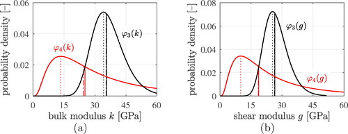
The equivalent piecewise uniform microelastic values are very close to the median values. This provides the motivation to use the median values as input for the piecewise uniform microelastic model.

4.3. Piecewise uniform microelastic model fed with median values of the two populations of hydrate bulk and shear moduli

The median values of Eqs. (100)(100) $$\text{median}(k_3)=35.61\text{GPa},\text{median}(g_3)=26.52\text{GPa},$$(100) and (101)(101) $$\text{median}(k_4)=25.19\text{GPa},\text{median}(g_4)=18.76\text{GPa}.$$(101) are assigned to the LDCR and to the HDCR hydrates. The elastic properties of zirconia and clinker as well as the volume fractions of all constituents are taken from Table 2, the crack density parameter from Eq. (60)(60) $$\omega =0.7802,$$(60) . Corresponding homogenized stiffness properties of Biodentine are obtained for the stiffness moduli from Eqs. (82)(82) $$k_{\mathit{bio}}=\left\{\sum _{i=1}^4\frac{f_i{k}_i}{1+\frac{S_{\mathit{vol}}(k_i-k_{\mathit{bio}})}{k_{\mathit{bio}}}}\right\}\times {\{\sum _{i=1}^4\frac{f_i}{1+\frac{S_{\mathit{vol}}(k_i-k_{\mathit{bio}})}{k_{\mathit{bio}}}}\}}^{-1},$$(82) and (83)(83) $$g_{\mathit{bio}}=\left\{\sum _{i=1}^4\frac{f_i{g}_i}{1+\frac{S_{\mathit{dev}}(g_i-g_{\mathit{bio}})}{g_{\mathit{bio}}}}\right\}\times {\{\sum _{i=1}^4\frac{f_i}{1+\frac{S_{\mathit{dev}}(g_i-g_{\mathit{bio}})}{g_{\mathit{bio}}}}+\frac{4\pi \omega }{3}{T}_{\mathit{dev}}\}}^{-1},$$(83) : (102) $$k_{\mathit{bio}}=38.72\text{GPa},g_{\mathit{bio}}=14.17\text{GPa}.$$(102) These median-based values are by only 0.8% and 0.5% larger than the corresponding values of the lognormal microelasticity model: $k_{\mathit{bio}}=38.4\text{GPa},$ and $g_{\mathit{bio}}=14.1\text{GPa},$ respectively. The (population-averaged) strain and stress concentration tensor components of the piecewise uniform median-based microelasticity model, computed according to Eqs. (84)–(87), are listed in Tables 8 and 9. They differ from the reference values of the lognormal microelasticity model, see Tables 4 and 5, by only up to 1.05%.

Table 8. Results of the median-based piecewise uniform microelasticity model: strain concentration tensors components of the four types of solid constituents of Biodentine according to Eqs. (84)(84) $$A_{\mathit{vol},j}=\frac{1}{1+\frac{S_{\mathit{vol}}(k_j-k_{\mathit{bio}})}{k_{\mathit{bio}}}}\times {\left\{\sum _{i=1}^4\frac{f_i}{1+\frac{S_{\mathit{vol}}(k_i-k_{\mathit{bio}})}{k_{\mathit{bio}}}}\right\}}^{-1},$$(84) and (85)(85) $$A_{\mathit{dev},j}=\frac{1}{1+\frac{S_{\mathit{dev}}(g_j-g_{\mathit{bio}})}{g_{\mathit{bio}}}}\times {\{\sum _{i=1}^4\frac{f_i}{1+\frac{S_{\mathit{dev}}(g_i-g_{\mathit{bio}})}{g_{\mathit{bio}}}}+\frac{4\pi \omega }{3}{T}_{\mathit{dev}}\}}^{-1},$$(85) . The differences of the $A_{\mathit{vol},i},$ and $A_{\mathit{dev},i}$ values to the lognormal model are given in brackets.

Constituent of Biodentine	Strain concentration tensor components and deviations from lognormal microelasticity model
zirconia	$A_{\mathit{vol},1}=0.3036\hspace{1em}(-0.63\%)$	$A_{\mathit{dev},1}=0.2362\hspace{1em}(-0.43\%)$
clinker	$A_{\mathit{vol},2}=0.4250\hspace{1em}(-0.64\%)$	$A_{\mathit{dev},2}=0.3204\hspace{1em}(-0.38\%)$
HDCR hydrates	$A_{\mathit{vol},3}=1.0570\hspace{1em}(-0.18\%)$	$A_{\mathit{dev},3}=0.5250\hspace{1em}(-0.04\%)$
LDCR hydrates	$A_{\mathit{vol},4}=1.3068\hspace{1em}(+1.05\%)$	$A_{\mathit{dev},4}=0.6414\hspace{1em}(+0.22\%)$

Table 9. Results of the median-based piecewise uniform microelasticity model: stress concentration tensors components of the four types of solid constituents of Biodentine according to Eqs. (86)(86) $$B_{\mathit{vol},j}=\frac{k_j/k_{\mathit{bio}}}{1+\frac{S_{\mathit{vol}}(k_j-k_{\mathit{bio}})}{k_{\mathit{bio}}}}\times {\left\{\sum _{i=1}^4\frac{f_i}{1+\frac{S_{\mathit{vol}}(k_i-k_{\mathit{bio}})}{k_{\mathit{bio}}}}\right\}}^{-1},$$(86) and (87)(87) $$B_{\mathit{dev},j}=\frac{g_j/g_{\mathit{bio}}}{1+\frac{S_{\mathit{dev}}(g_j-g_{\mathit{bio}})}{g_{\mathit{bio}}}}\times {\{\sum _{i=1}^4\frac{f_i}{1+\frac{S_{\mathit{dev}}(g_i-g_{\mathit{bio}})}{g_{\mathit{bio}}}}+\frac{4\pi \omega }{3}{T}_{\mathit{dev}}\}}^{-1}.$$(87) . The differences of the $B_{\mathit{vol},i},$ and $B_{\mathit{dev},i}$ values to the lognormal model are given in brackets.

Constituent of Biodentine	Stress concentration tensor components and deviations from lognormal microelasticity model
zirconia	$B_{\mathit{vol},1}=1.3397\hspace{1em}(+0.16\%)$	$B_{\mathit{dev},1}=1.3397\hspace{1em}(+0.06\%)$
clinker	$B_{\mathit{vol},2}=1.2805\hspace{1em}(+0.18\%)$	$B_{\mathit{dev},2}=1.2805\hspace{1em}(+0.08\%)$
HDCR hydrates	$B_{\mathit{vol},3}=0.9722\hspace{1em}(+0.08\%)$	$B_{\mathit{dev},3}=0.9722\hspace{1em}(+0.01\%)$
LDCR hydrates	$B_{\mathit{vol},4}=0.8503\hspace{1em}(-0.87\%)$	$B_{\mathit{dev},4}=0.8503\hspace{1em}(-0.20\%)$

5. Discussion

Herein, the solid constituents of Biodentine were modeled as spherical phases, such as introduced in the first micromechanics models for cementitious materials [4, 36]. Stora et al. [37] scrutinized this approach and found that spherical shapes are suitable for hardened cement pastes, but questionable for leached pastes with porosities of up to 40%. Sanahuja et al. [38] identified specific aspect ratios of oblate nanoscopic solid C-S-H building blocks, in order to model setting (= transition from a gel-like suspension to a solid material). Pichler et al. [39] compared spherical and prolate shapes assigned to micron-sized gel-porous hydrates and found significant differences at early ages, when the porosity is quite large, but small differences at mature ages, when the microstructure is already rather dense. Because the present paper refers to well-hardened Biodentine, spherical phase shapes are suitable for micromechanical modeling.

The identified value of Poisson’s ratio of the calcite-reinforced hydrates of Biodentine (${\nu }_h=0.20$) is smaller than 0.24 which is the value standardly assumed for low-density and high-density C-S-H of construction cement pastes [5]. This difference can be explained from the compositional characteristics of the hydrates found in construction cement pastes and in Biodentine, respectively. Low-density and high-density C-S-H consist of solid C-S-H building blocks and pores [40]. Calcite-reinforced hydrates of Biodentine, in turn, consist of solid C-S-H building blocks, pores, calcium hydroxide, and calcite. Thus, they are somewhat reminiscent of a composite initially referred to as “ultra-high-density C-S-H” [41], which turned out to be a high-density C-S-H reinforced by small crystals of calcium hydroxide [42], see also [43–45].

The present paper continues the line of studies in which results from nanoindentation were combined with micromechanical homogenization approaches. Sorelli et al. [46] applied the method of Constantinides and Ulm [4] to an ultra-high performance concrete, Němeček et al. [47] to cement paste, gypsum, and an aluminum alloy, and Göbel et al. [48] to polymer-modified cement paste. Other complementary research approaches combined grid nanoindentation and stiffness homogenization at different scales of observation and with different targets, as will be discussed next. As for the smallest scales, scanning electron microscopy, energy dispersive spectroscopy, and X-ray diffraction were combined to gain access to the composition at nanoindented material points, and this knowledge was upscaled by means of homogenization methods in order to predict the stiffness at the indented material points, see e.g. [44, 49]. At the next larger scale, microstructural properties of cement paste determined by means of grid nanoindentation were used as input for stiffness upscaling, in order to predict stiffness properties determined by means of microindentation, see e.g. [50]. As for stiffness homogenization up to the material scale of concrete, grid nanoindentation, used for quantifying microstructural properties of cement paste, was combined with microindentation, used for the characterization of interfacial transition zones surrounding aggregates, see e.g. [51].

The present study shares two aspects of emerging developments regarding stiffness upscaling based on results obtained from grid nanoindentation. The first one relates to using probability density functions describing stiffness distributions of two populations of hydrate phases as input for micromechanical modeling, as realized by Stefaniuk et al. [52] for symmetric, Gaussian stiffness distributions. In this context, our current approach goes three steps further, (i) employing lognormal rather than Gaussian distributions, (ii) evaluating corresponding concentration relations revealing the microstresses to follow generalized beta distributions, and (iii) identifying that median values of the skewed stiffness distributions are representative piecewise uniform stiffness properties governing the overall stiffness of Biodentine. The second aspect relates to weak interfaces. Liang et al. [53] and Damien et al. [54] have used a modified Eshelby tensor in the context of cementitious matrix-inclusion composites homogenized by means of the Mori-Tanaka scheme [55], in order to account for weak tangential bond in interfaces between spherical phases and the surrounding matrix. Herein, we have modeled weak grain boundaries by means of closed circular microcracks which are isotropically oriented in space, in the context of homogenizing the “polycrystalline” microstructure of Biodentine by means of the self-consistent scheme [26]. This approach allowed us to show that almost 50% of the deformation of hardened Biodentine refers to shear-dislocations of weak grain boundaries.

6. Conclusions

A lognormal microelasticity model for hardened Biodentine was based on the results of a grid nanoindentation campaign. Poisson’s ratio of the two populations of hydrates and the crack density parameter were identified such that the model reproduces macroscopic stiffness properties derived from ultrasonic pulse velocity measurements. Based on the results of the presented study, the following conclusions are drawn:

• The identified value of Poisson’s ratio of the lower-density and high-density calcite-reinforced hydrates of Biodentine, ${\nu }_h=0.20,$ is smaller than Poisson’s ratio used for the low-density and high-density calcium-silicate-hydrates of Portland cements: $\nu =0.24,$ see [4]. The difference is attributed to a reinforcement effect of calcite and calcium hydroxide.

• Grain boundary defects (modeled as microcracks) are responsible for almost 50% of the deviatoric deformation of Biodentine. The corresponding value of the crack density parameter was identified as $\omega =0.78.$

• Bottom-up stiffness homogenization, accounting for microscopic stiffness distributions of the hydrates, is virtually equivalent to upscaling of piecewise uniform stiffness properties, provided that medians of the microscopic stiffness distributions are assigned to the hydrates. Corresponding differences regarding the homogenized stiffness of Biodentine were found to be smaller than 1.1%. This corroborates the validity of standard homogenization models for the elastic stiffness of cementitious materials, because these models are based on piecewise uniform stiffness properties.

• As for top-down strain and stress quantification, there are important differences between the lognormal micro-elasticity model and the alternative which is based on piecewise uniform microscopic stiffness values. The latter approach leads to volume-averaged values of the stresses experienced by the two populations of hydrates. The statistical homogenization approach, in turn, provides direct access to microscopic stress fluctuations. These fluctuations are expected to be valuable for future strength modeling, which, however, goes beyond the scope of the present paper.

Acknowledgment

The authors gratefully acknowledge the support of Olaf Lahayne from the Institute for Mechanics of Materials and Structures, TU Wien, concerning the ultrasound experiments.

Additional information

Funding

This project has received funding from the European Union’s Horizon 2020 research and innovation program under the Marie Skłodowska-Curie Grant Agreement No. 764691.

Notes

1 The transition to flat circular slit cracks will be explained in Subsection 2.3.

2 The value of ν_h will be identified in Subsection 2.7.

Appendix A

Macrostiffness characterization by means of ultrasonic pulse velocity measurements

The ultrasonic pulse transmission method was used as nondestructive technique to characterize the macroscopic elastic properties of hardened Biodentine. Here, both longitudinal and shear waves, with excitation frequencies ranging from 50 kHz to 20 MHz, were sent through cylindrical Biodentine samples with 5 mm diameter and 10 mm height.

The test setup consisted of a serial arrangement of a pulse generator, a layer of coupling medium (honey), a plastic foil, the specimen, another plastic foil, another layer of honey, and a pulse detector. The plastic foils protected the sample against contamination of its open porosity with the coupling medium. The specimens, the equipment, and its surrounding environment were conditioned to 37 °C.

The wave velocities v of Biodentine are equal to the height b of the tested specimens divided by the time of flight t_f of the ultrasonic pulse through the tested specimen, (A.1) $$v=\frac{b}{t_f}.$$(A.1) Direct measurement of t_f is not possible; however, it results from the difference of two other time measurements, (A.2) $$t_f=t_{\mathit{tot}}-t_d,$$(A.2) where t_tot is the travel time of the pulse from the transducer – through the coupling medium, the plastic foils, and the specimen – to the receiver, while the delay time t_d is needed by the pulse to just travel from the generator, through honey and plastic foils (without specimen), to the receiver.

Figure A.12. Longitudinal and shear wave velocities sent at different frequencies through cylindrical samples of Biodentine, with 5 mm diameter and 10 mm height; the mean longitudinal wave velocity is equal to ${\overline{v}}_L=4.977$ km/s (upper data points cluster) and the mean shear wave velocity amounts to ${\overline{v}}_S=2.473$ km/s (lower data points cluster). The pink markers correspond to 50 kHz transducers central frequency, red to 500 kHz, cyan to 1 MHz, black to 2.25 MHz, green to 5 MHz, blue to 10 MHz, and yellow to 20 MHz transducers’ central frequency, after [3].

325 measurements of longitudinal waves were performed at material ages from 7 to 28 days [3]. The central excitation frequencies amounted to 50 kHz, 500 kHz, 1 MHz, 2.25 MHz, 5 MHz, 10 MHz, and 20 MHz. The longitudinal wave velocities were fairly independent of the material age as well as the testing frequency. On average, they amount to ${\overline{v}}_L=4.977$ km/s, see [3] and Fig. A.12.

122 measurements of shear waves were performed at material ages from 7 to 28 days. The central excitation frequencies amounted to 2.25 MHz and 5 MHz, see Table A.10. The shear wave velocities are also fairly independent of the material age and the testing frequency. On average, they amount to ${\overline{v}}_S=2.473$ km/s, see Fig. A.12.

Table A.10. Ultrasonic shear wave transducers used for characterization of hardened Biodentine.

Frequency [MHz]	Shear transducer
2.25	V154-RM
5	V155-RM

The separation of scales principle states that the wavelengths λ must be significantly larger than the size ${\ell }_{\mathit{rve}}$ of a representative volume element of the tested material [26, 56], and that ${\ell }_{\mathit{rve}}$ must be significantly larger than the characteristic size ${\ell }_{\mathit{het}}$ of the microheterogeneities: (A.3) $$\lambda \gg {\ell }_{\mathit{rve}}\gg {\ell }_{\mathit{het}}.$$(A.3) Residual clinker grains are the largest microheterogeneities of hardened Biodentine. Their characteristic size amounts to 4.3 μm [3]. Thus, ${\ell }_{\mathit{het}}=4.3\mathrm{\mu }\mathrm{m}.$ The characteristic size of a representative volume of Biodentine is some three times larger [57, 58]. Thus, ${\ell }_{\mathit{rve}}=12.9\mathrm{\mu }$m. This size is to be compared with the wavelengths of the ultrasonic pulses.

The wavelength is indirectly proportional to the ultrasonic frequency. Therefore, the largest testing frequency yields a lower bound for the wavelengths. As for the longitudinal waves, this lower bound follows as (A.4) $${\lambda }_L\ge \frac{{\overline{v}}_L}{\mathrm{max\hspace{0.17em}}f}=\frac{4.977\text{km}/\mathrm{s}}{20\text{MHz}}=249\mathrm{\mu }\mathrm{m}.$$(A.4) As for the shear waves, it follows as (A.5) $${\lambda }_S\ge \frac{{\overline{v}}_S}{\mathrm{max\hspace{0.17em}}f}=\frac{2.473\text{km}/\mathrm{s}}{5\text{MHz}}=495\mathrm{\mu }\mathrm{m}.$$(A.5) Eqs. (A.4)(A.4) $${\lambda }_L\ge \frac{{\overline{v}}_L}{\mathrm{max\hspace{0.17em}}f}=\frac{4.977\text{km}/\mathrm{s}}{20\text{MHz}}=249\mathrm{\mu }\mathrm{m}.$$(A.4) and (A.5)(A.5) $${\lambda }_S\ge \frac{{\overline{v}}_S}{\mathrm{max\hspace{0.17em}}f}=\frac{2.473\text{km}/\mathrm{s}}{5\text{MHz}}=495\mathrm{\mu }\mathrm{m}.$$(A.5) underline that the wavelengths were by a factor of 19 (longitudinal waves) and 38 (shear waves) larger than ${\ell }_{\mathit{rve}}=12.9\mathrm{\mu }$m. The principle of separation of scales, see Eq. (A.3)(A.3) $$\lambda \gg {\ell }_{\mathit{rve}}\gg {\ell }_{\mathit{het}}.$$(A.3) , is fulfilled [26, 56]. This provides evidence that wave velocities of Fig. A.12 are representative for the homogenized composite Biodentine.

According to the theory of wave propagation through isotropic linear-elastic media, longitudinal and shear wave velocities, together with the mass density ρ of the tested material, allow for quantifying the bulk modulus, k, and the shear modulus, g, as [59–61], (A.6) $$k^{\hspace{0.17em}\mathit{\text{exp}}\hspace{0.17em}}=\frac{\rho }{3}\left(3{\overline{v}}_L^2-4{\overline{v}}_S^2\right),$$(A.6) (A.7) $$g^{\hspace{0.17em}\mathit{\text{exp}}\hspace{0.17em}}=\rho {\overline{v}}_S^2,$$(A.7) respectively. Evaluation of Eqs. (A.6)(A.6) $$k^{\hspace{0.17em}\mathit{\text{exp}}\hspace{0.17em}}=\frac{\rho }{3}\left(3{\overline{v}}_L^2-4{\overline{v}}_S^2\right),$$(A.6) and (A.7)(A.7) $$g^{\hspace{0.17em}\mathit{\text{exp}}\hspace{0.17em}}=\rho {\overline{v}}_S^2,$$(A.7) based on $\rho =2.311{\text{kg}/\text{dm}}^3$ [3] and the wave velocities of Fig. A.12 gives access to constant isotropic elastic properties, namely to a bulk modulus of 38.4 GPa and a shear modulus of 14.1 GPa.

Appendix B

Numerical values of integrals involving the lognormal distributions of the two populations of hydrates

Numerical evaluation of the integrals in Eqs. (41)(41) $$\begin{array}{c}{k}_{\mathit{bio}}=\{\sum _{i=1}^2\frac{f_i{k}_i}{1+\frac{S_{\mathit{vol}}(k_i-k_{\mathit{bio}})}{k_{\mathit{bio}}}}+\sum _{i=3}^4{f}_i\underset{0}{\overset{\infty }{\int }}\frac{{\phi }_i(M)k_i(M)}{1+\frac{S_{\mathit{vol}}(k_i(M)-k_{\mathit{bio}})}{k_{\mathit{bio}}}} \mathrm{d}M\}\\ \times {\{\sum _{i=1}^2\frac{f_i}{1+\frac{S_{\mathit{vol}}(k_i-k_{\mathit{bio}})}{k_{\mathit{bio}}}}+\sum _{i=3}^4{f}_i\mathrm{ }\underset{0}{\overset{\infty }{\int }}\frac{{\phi }_i(M)}{1+\frac{S_{\mathit{vol}}(k_i(M)-k_{\mathit{bio}})}{k_{\mathit{bio}}}} \mathrm{d}M\}}^{-1},\end{array}$$(41) , (42)(42) $$\begin{array}{c}{g}_{\mathit{bio}}=\{\sum _{i=1}^2\frac{f_i{g}_i}{1+\frac{S_{\mathit{dev}}(g_i-g_{\mathit{bio}})}{g_{\mathit{bio}}}}+\sum _{i=3}^4{f}_i\underset{0}{\overset{\infty }{\int }}\frac{{\phi }_i(M)g_i(M)}{1+\frac{S_{\mathit{dev}}(g_i(M)-g_{\mathit{bio}})}{g_{\mathit{bio}}}} \mathrm{d}M\}\\ \times \{\sum _{i=1}^2\frac{f_i}{1+\frac{S_{\mathit{dev}}(g_i-g_{\mathit{bio}})}{g_{\mathit{bio}}}}+\sum _{i=3}^4{f}_i\underset{0}{\overset{\infty }{\int }}\frac{{\phi }_i(M)}{1+\frac{S_{\mathit{dev}}(g_i(M)-g_{\mathit{bio}})}{g_{\mathit{bio}}}} \mathrm{d}M\\ \hspace{1em}+\frac{4\pi \omega }{3}{T}_{\mathit{dev}}{\}}^{-1}.\end{array}$$(42) , (44)–(47), and (51)–(54), based on $k_{\mathit{bio}}=38.4\text{GPa},g_{\mathit{bio}}=14.1\text{GPa},$ and ${\nu }_h=0.2017,$ delivers the following numerical results: (B.1) $$\underset{0}{\overset{\infty }{\int }}\frac{{\phi }_3(M)k_3(M)}{1+\frac{S_{\mathit{vol}}(k_3(M)-k_{\mathit{bio}})}{k_{\mathit{bio}}}} \mathrm{d}M=37.36450836\text{GPa},$$(B.1) (B.2) $$\underset{0}{\overset{\infty }{\int }}\frac{{\phi }_4(M)k_4(M)}{1+\frac{S_{\mathit{vol}}(k_4(M)-k_{\mathit{bio}})}{k_{\mathit{bio}}}} \mathrm{d}M=32.37198195\text{GPa},$$(B.2) (B.3) $$\underset{0}{\overset{\infty }{\int }}\frac{{\phi }_3(M)}{1+\frac{S_{\mathit{vol}}(k_3(M)-k_{\mathit{bio}})}{k_{\mathit{bio}}}} \mathrm{d}M=1.05507934,$$(B.3) (B.4) $$\underset{0}{\overset{\infty }{\int }}\frac{{\phi }_4(M)}{1+\frac{S_{\mathit{vol}}(k_4(M)-k_{\mathit{bio}})}{k_{\mathit{bio}}}} \mathrm{d}M=1.32063926,$$(B.4) (B.5) $$\underset{0}{\overset{\infty }{\int }}\frac{{\phi }_3(M)g_3(M)}{1+\frac{S_{\mathit{dev}}(g_3(M)-g_{\mathit{bio}})}{g_{\mathit{bio}}}} \mathrm{d}M=18.77600304\text{GPa},$$(B.5) (B.6) $$\underset{0}{\overset{\infty }{\int }}\frac{{\phi }_4(M)g_4(M)}{1+\frac{S_{\mathit{dev}}(g_4(M)-g_{\mathit{bio}})}{g_{\mathit{bio}}}} \mathrm{d}M=16.19052283\text{GPa},$$(B.6) (B.7) $$\underset{0}{\overset{\infty }{\int }}\frac{{\phi }_3(M)}{1+\frac{S_{\mathit{dev}}(g_3(M)-g_{\mathit{bio}})}{g_{\mathit{bio}}}} \mathrm{d}M=0.71090769,$$(B.7) (B.8) $$\underset{0}{\overset{\infty }{\int }}\frac{{\phi }_4(M)}{1+\frac{S_{\mathit{dev}}(g_4(M)-g_{\mathit{bio}})}{g_{\mathit{bio}}}} \mathrm{d}M=0.87075413.$$(B.8)

Appendix C

Components of the Eshelby tensor of thin oblate spheroids

Consider a thin oblate spheroid with the unit normal to the “crack” plane parallel to ${\mathbf{e}}_3.$ The non-vanishing components of the Eshelby tensor ${\mathbb{S}}_{\mathit{obl}}$ read as [31] (C.1) $$\begin{array}{c}{S}_{1111}=\frac{3}{16}\frac{9k_{\mathit{bio}}+7g_{\mathit{bio}}}{3k_{\mathit{bio}}+4g_{\mathit{bio}}}\pi X,S_{2211}=S_{1122},\\ S_{1122}=\frac{9}{16}\frac{k_{\mathit{bio}}-g_{\mathit{bio}}}{3k_{\mathit{bio}}+4g_{\mathit{bio}}}\pi X,S_{2222}=S_{1111},\\ S_{1133}=\frac{3}{4}\frac{-g_{\mathit{bio}}}{3k_{\mathit{bio}}+4g_{\mathit{bio}}}\pi X,S_{2233}=S_{1133},\\ S_{3311}=\frac{3}{4}\frac{g_{\mathit{bio}}-3k_{\mathit{bio}}}{4g_{\mathit{bio}}+3k_{\mathit{bio}}}\pi X-\frac{2g_{\mathit{bio}}-3k_{\mathit{bio}}}{4g_{\mathit{bio}}+3k_{\mathit{bio}}},S_{1212}=\frac{3}{16}\frac{3k_{\mathit{bio}}+5g_{\mathit{bio}}}{3k_{\mathit{bio}}+4g_{\mathit{bio}}}\pi X,S_{3322}=S_{3311}{S}_{2323}=\frac{1}{2}\left(1-\frac{3}{4}\frac{3k_{\mathit{bio}}+2g_{\mathit{bio}}}{3k_{\mathit{bio}}+4g_{\mathit{bio}}}\pi X\right),\\ S_{3333}=1-\frac{3g_{\mathit{bio}}}{2(3k_{\mathit{bio}}+4g_{\mathit{bio}})}\pi X,S_{3131}=S_{2323},\end{array}$$(C.1) with $S_{\mathit{ijkl}}=S_{\mathit{jikl}}=S_{\mathit{ijlk}}.$ Notably, $X=c/a$ denotes the aspect ratio.

References

- P. Laurent, J. Camps, M. De Méo, J. Déjou, and I. About , Induction of specific cell responses to a Ca3SiO5-based posterior restorative material, Dent Mater., vol. 24, no. 11, pp. 1486–1494, 2008. DOI: 10.1016/j.dental.2008.02.020.
- P. Laurent, and J. Camps, Biodentine induces TGF-β1 release from human pulp cells and early dental pulp mineralization, Int. Endodon. J., vol. 45, no. 5, pp. 439–448, 2012. DOI: 10.1111/j.1365-2591.2011.01995.x
- P. Dohnalík, B.L. Pichler, L. Zelaya-Lainez, O. Lahayne, G. Richard, and C. Hellmich, Micromechanics of dental cement paste, J. Mech. Behav. Biomed. Mater., vol. 124, pp. 104863, 2021. DOI: 10.1016/j.jmbbm.2021.104863.
- G. Constantinides, and F.-J. Ulm, The effect of two types of C-S-H on the elasticity of cement-based materials: Results from nanoindentation and micromechanical modeling, Cement Concrete Res., vol. 34, no. 1, pp. 67–80, 2004. DOI: 10.1016/S0008-8846(03)00230-8.
- G. Constantinides, The elastic properties of calcium leached cement pastes and mortars: A multi-scale investigation, Master’s thesis, Massachusetts Institute of Technology, 2002.
- M. Miller, C. Bobko, M. Vandamme, and F.-J. Ulm, Surface roughness criteria for cement paste nanoindentation, Cement Concrete Res., vol. 38, no. 4, pp. 467–476, 2008. DOI: 10.1016/j.cemconres.2007.11.014.
- E. Donnelly, S.P. Baker, A.L. Boskey, and M.C. van der Meulen, Effects of surface roughness and maximum load on the mechanical properties of cancellous bone measured by nanoindentation, J. Biomed. Mater. Res. A., vol. 77, no. 2, pp. 426–435, 2006. DOI: 10.1002/jbm.a.30633.
- W.C. Oliver, and G.M. Pharr, An improved technique for determining hardness and elastic modulus using load and displacement sensing indentation experiments, J. Mater. Res., vol. 7, no. 6, pp. 1564–1583, 1992. DOI: 10.1557/JMR.1992.1564.
- Q. Li, A.P. Hurt, and N.J. Coleman, The application of 29Si NMR spectroscopy to the analysis of calcium silicate-based cement using Biodentine as an example, JFB, vol. 10, no. 2, pp. 25, 2019. DOI: 10.3390/jfb10020025.
- J. Taplin, A method for following the hydration reaction in Portland cement paste, Austral. J. Appl. Sci., vol. 10, pp. 329–345, 1959.
- S. Diamond, and D. Bonen, Microstructure of hardened cement paste—a new interpretation, J. Am. Ceram. Soc., vol. 76, no. 12, pp. 2993–2999, 1993. DOI: 10.1111/j.1151-2916.1993.tb06600.x.
- P.D. Tennis, and H.M. Jennings, A model for two types of calcium silicate hydrate in the microstructure of Portland cement pastes, Cement Concrete Res., vol. 30, no. 6, pp. 855–863, 2000. DOI: 10.1016/S0008-8846(00)00257-X.
- H.M. Jennings, A model for the microstructure of calcium silicate hydrate in cement paste, Cement Concrete Res., vol. 30, no. 1, pp. 101–116, 2000. DOI: 10.1016/S0008-8846(99)00209-4.
- M. Königsberger, C. Hellmich, and B. Pichler, Densification of C-S-H is mainly driven by available precipitation space, as quantified through an analytical cement hydration model based on NMR data, Cement Concrete Res., vol. 88, pp. 170–183, 2016. DOI: 10.1016/j.cemconres.2016.04.006.
- Y. Ma, G. Ye, and J. Hu, Micro-mechanical properties of alkali-activated fly ash evaluated by nanoindentation, Construct. Build. Mater., vol. 147, pp. 407–416, 2017. DOI: 10.1016/j.conbuildmat.2017.04.176.
- M. Königsberger, L. Zelaya-Lainez, O. Lahayne, B.L. Pichler, and C. Hellmich, Nanoindentation-probed Oliver-Pharr half-spaces in alkali-activated slag-fly ash pastes: Multimethod identification of microelasticity and hardness, Mech. Adv. Mater. Struct., vol. 2021, pp. 1–12, 2021. DOI: 10.1080/15376494.2021.1941450.
- R.J. Hussey, and J. Wilson, Advanced Technical Ceramics Directory and Databook, Springer Science & Business Media, Berlin, Heidelberg, 1998.
- B. Pichler, and C. Hellmich, Upscaling quasi-brittle strength of cement paste and mortar: A multi-scale engineering mechanics model, Cement Concrete Res., vol. 41, no. 5, pp. 467–476, 2011. DOI: 10.1016/j.cemconres.2011.01.010.
- B. Budiansky, and R.J. O’Connell, Elastic moduli of a cracked solid, Int. J. Solids Struct., vol. 12, no. 2, pp. 81–97, 1976. DOI: 10.1016/0020-7683(76)90044-5.
- V. Pensée, D. Kondo, and L. Dormieux, Micromechanical analysis of anisotropic damage in brittle materials, J. Eng. Mech., vol. 128, no. 8, pp. 889–897, 2002. DOI: 10.1061/(ASCE)0733-9399(2002)128:8(889).
- Z. Hashin, Analysis of composite materials—a survey, J. Appl. Mech., vol. 50, no. 3, pp. 481–505, 1983. DOI: 10.1115/1.3167081.
- M. Königsberger, B. Pichler, and C. Hellmich, Multiscale poro-elasticity of densifying calcium-silicate hydrates in cement paste: An experimentally validated continuum micromechanics approach, Int. J. Eng. Sci., vol. 147, pp. 103196, 2020. DOI: 10.1016/j.ijengsci.2019.103196.
- R. Hill, Elastic properties of reinforced solids: Some theoretical principles, J. Mech. Phys. Solids, vol. 11, no. 5, pp. 357–372, 1963. DOI: 10.1016/0022-5096(63)90036-X.
- R. Hill, Continuum micro-mechanics of elastoplastic polycrystals, J. Mech. Phys. Solids, vol. 13, no. 2, pp. 89–101, 1965. DOI: 10.1016/0022-5096(65)90023-2.
- R. Hill, A self-consistent mechanics of composite materials, J. Mech. Phys. Solids, vol. 13, no. 4, pp. 213–222, 1965. DOI: 10.1016/0022-5096(65)90010-4.
- A. Zaoui, Continuum micromechanics: Survey, J. Eng. Mech., vol. 128, no. 8, pp. 808–816, 2002. DOI: 10.1061/(ASCE)0733-9399(2002)128:8(808).
- J.D. Eshelby, The determination of the elastic field of an ellipsoidal inclusion, and related problems, Proc. R. Soc. Lond.: Ser. A. 396, vol. 241, no. 1226, pp. 376, 1957. DOI: 10.1098/rspa.1957.0133
- N. Laws, The determination of stress and strain concentrations at an ellipsoidal inclusion in an anisotropic material, J. Elasticity, vol. 7, no. 1, pp. 91–97, 1977. DOI: 10.1007/BF00041133.
- L. Dormieux, D. Kondo, and F.-J. Ulm, Microporomechanics, John Wiley & Sons, Hoboken, NJ, 2006.
- Q.-Z. Zhu, J. Shao, and D. Kondo, A micromechanics-based thermodynamic formulation of isotropic damage with unilateral and friction effects, Eur. J. Mech. A. Solids, vol. 30, no. 3, pp. 316–325, 2011. DOI: 10.1016/j.euromechsol.2010.12.005.
- B. Pichler, C. Hellmich, and H.A. Mang, A combined fracture-micromechanics model for tensile strain-softening in brittle materials, based on propagation of interacting microcracks, Int. J. Numer. Anal. Meth. Geomech., vol. 31, no. 2, pp. 111–132, 2007. DOI: 10.1002/nag.544.
- V. Deudé, L. Dormieux, D. Kondo, and S. Maghous, Micromechanical approach to nonlinear poroelasticity: Application to cracked rocks, J. Eng. Mech., vol. 128, no. 8, pp. 848–855, 2002. DOI: 10.1061/(ASCE)0733-9399(2002)128:8(848).
- M. Irfan-ul-Hassan, B. Pichler, R. Reihsner, and C. Hellmich, Elastic and creep properties of young cement paste, as determined from hourly repeated minute-long quasi-static tests, Cement Concrete Res., vol. 82, pp. 36–49, 2016. DOI: 10.1016/j.cemconres.2015.11.007.
- D. Johnson, The triangular distribution as a proxy for the beta distribution in risk analysis, J. R. Statist. Soc. D., vol. 46, no. 3, pp. 387–398, 1997. DOI: 10.1111/1467-9884.00091.
- M.A. Chaudhry, A. Qadir, M. Rafique, and S. Zubair, Extension of Euler’s beta function, J. Comput. Appl. Math., vol. 78, no. 1, pp. 19–32, 1997. DOI: 10.1016/S0377-0427(96)00102-1.
- O. Bernard, F.-J. Ulm, and E. Lemarchand, A multiscale micromechanics-hydration model for the early-age elastic properties of cement-based materials, Cement Concrete Res., vol. 33, no. 9, pp. 1293–1309, 2003. DOI: 10.1016/S0008-8846(03)00039-5.
- E. Stora, Q.-C. He, and B. Bary, Influence of inclusion shapes on the effective linear elastic properties of hardened cement pastes, Cement Concrete Res., vol. 36, no. 7, pp. 1330–1344, 2006. DOI: 10.1016/j.cemconres.2006.02.007.
- J. Sanahuja, L. Dormieux, and G. Chanvillard, Modelling elasticity of a hydrating cement paste, Cement Concrete Res., vol. 37, no. 10, pp. 1427–1439, 2007. DOI: 10.1016/j.cemconres.2007.07.003.
- B. Pichler, C. Hellmich, and J. Eberhardsteiner, Spherical and acicular representation of hydrates in a micromechanical model for cement paste: Prediction of early-age elasticity and strength, Acta Mech., vol. 203, no. 3–4, pp. 137–162, 2009. DOI: 10.1007/s00707-008-0007-9.
- G. Constantinides, F.-J. Ulm, and K. Van Vliet, On the use of nanoindentation for cementitious materials, Mat. Struct., vol. 36, no. 3, pp. 191–196, 2003. DOI: 10.1007/BF02479557.
- M. Vandamme, and F.-J. Ulm, Nanogranular origin of concrete creep, Proc. Natl. Acad. Sci. U. S. A., vol. 106, no. 26, pp. 10552–10557, 2009. DOI: 10.1073/pnas.0901033106.
- J.J. Chen, L. Sorelli, M. Vandamme, F.-J. Ulm, and G. Chanvillard, A coupled nanoindentation/SEM-EDS study on low water/cement ratio Portland cement paste: Evidence for C-S-H/Ca(OH)2 nanocomposites, J. Am. Ceram. Soc., vol. 93, no. 5, pp. 1484–1493, 2010. DOI: 10.1111/j.1551-2916.2009.03599.x.
- W. Da Silva, J. Němeček, and P. Štemberk, Methodology for nanoindentation-assisted prediction of macroscale elastic properties of high performance cementitious composites, Cement Concrete Res., vol. 45, pp. 57–68, 2014. DOI: 10.1016/j.cemconcomp.2013.09.013.
- L. Brown, P.G. Allison, and F. Sanchez, Use of nanoindentation phase characterization and homogenization to estimate the elastic modulus of heterogeneously decalcified cement pastes, Mater. Des., vol. 142, pp. 308–318, 2018. DOI: 10.1016/j.matdes.2018.01.030.
- E. Ford, A. Arora, B. Mobasher, C.G. Hoover, and N. Neithalath, Elucidating the nano-mechanical behavior of multi-component binders for ultra-high performance concrete, Construct. Build. Mater., vol. 243, pp. 118214, 2020. DOI: 10.1016/j.conbuildmat.2020.118214.
- L. Sorelli, G. Constantinides, F.-J. Ulm, and F. Toutlemonde, The nano-mechanical signature of ultra high performance concrete by statistical nanoindentation techniques, Cement Concrete Res., vol. 38, no. 12, pp. 1447–1456, 2008. DOI: 10.1016/j.cemconres.2008.09.002.
- J. Němeček, V. Králík, and J. Vondřejc, Micromechanical analysis of heterogeneous structural materials, Cement Concrete Compos., vol. 36, pp. 85–92, 2013. DOI: 10.1016/j.cemconcomp.2012.06.015.
- L. Göbel, C. Bos, R. Schwaiger, A. Flohr, and A. Osburg, Micromechanics-based investigation of the elastic properties of polymer-modified cementitious materials using nanoindentation and semi-analytical modeling, Cement Concrete Compos., vol. 88, pp. 100–114, 2018. DOI: 10.1016/j.cemconcomp.2018.01.010.
- Y. Li, P. Wang, and Z. Wang, Evaluation of elastic modulus of cement paste corroded in bring solution with advanced homogenization method, Construct. Build. Mater., vol. 157, pp. 600–609, 2017. DOI: 10.1016/j.conbuildmat.2017.09.133.
- X. Gao, Y. Wei, and W. Huang, Effect of individual phases on multiscale modeling mechanical properties of hardened cement paste, Construct. Build. Mater., vol. 153, pp. 25–35, 2017. DOI: 10.1016/j.conbuildmat.2017.07.074.
- Y. Li, Y. Liu, and R. Wang, Evaluation of the elastic modulus of concrete based on indentation test and multi-scale homogenization method, J. Build. Eng., vol. 43, pp. 102758, 2021. DOI: 10.1016/j.jobe.2021.102758.
- D. Stefaniuk, P. Niewiadomski, M. Musial, and D. Lydzba, Elastic properties of self-compacting concrete modified with nanoparticles: Multiscale approach, Arch. Civil Mech. Eng., vol. 19, no. 4, pp. 1150–1162, 2019. DOI: 10.1016/j.acme.2019.06.006.
- S. Liang, Y. Wei, and Z. Wu, Multiscale modeling elastic properties of cement-based materials considering imperfect interface effect, Construct. Build. Mater., vol. 154, pp. 567–579, 2017. DOI: 10.1016/j.conbuildmat.2017.07.196.
- D. Damien, Y. Wang, and Y. Xi, Prediction of elastic properties of cementitious materials based on multiphase and multiscale micromechanics theory, J. Eng. Mech., vol. 145, no. 10, pp. 04019074, 2019. DOI: 10.1061/(ASCE)EM.1943-7889.0001650.
- Y. Benveniste, A new approach to the application of Mori-Tanaka’s theory in composite materials, Mech. Mater., vol. 6, no. 2, pp. 147–157, 1987. DOI: 10.1016/0167-6636(87)90005-6.
- C. Kohlhauser, and C. Hellmich, Ultrasonic contact pulse transmission for elastic wave velocity and stiffness determination: Influence of specimen geometry and porosity, Eng. Struct., vol. 47, pp. 115–133, 2013. DOI: 10.1016/j.engstruct.2012.10.027.
- W. Drugan, and J. Willis, A micromechanics-based nonlocal constitutive equation and estimates of representative volume element size for elastic composites, J. Mech. Phys. Solids, vol. 44, no. 4, pp. 497–524, 1996. DOI: 10.1016/0022-5096(96)00007-5.
- V. Pensée, and Q.-C. He, Generalized self-consistent estimation of the apparent isotropic elastic moduli and minimum representative volume element size of heterogeneous media, Int. J. Solids Struct., vol. 44, no. 7-8, pp. 2225–2243, 2007. DOI: 10.1016/j.ijsolstr.2006.07.003.
- C. Kohlhauser, and C. Hellmich, Determination of Poisson’s ratios in isotropic, transversely isotropic, and orthotropic materials by means of combined ultrasonic-mechanical testing of normal stiffnesses: Application to metals and wood, Eur. J. Mech. A Solids, vol. 33, pp. 82–98, 2012. DOI: 10.1016/j.euromechsol.2011.11.009.
- J.M. Carcione, Wave fields in real media: Wave propagation in anisotropic, anelastic, porous and electromagnetic media, Elsevier, New York, NY, 2007.
- J. Achenbach, Wave propagation in elastic solids, One-dimensional motion of an elastic continuum, Elsevier, New York, NY, 1973.