Fast Calculating Surrogate Models for Leg and Head Impact in Vehicle–Pedestrian Collision Simulations

Abstract

Objective: In previous research, a tool chain to simulate vehicle–pedestrian accidents from ordinary driving state to in-crash has been developed. This tool chain allows for injury criteria-based, vehicle-specific (geometry, stiffness, active safety systems, etc.) assessments. Due to the complex nature of the included finite element analysis (FEA) models, calculation times are very high. This is a major drawback for using FEA models in large-scale effectiveness assessment studies. Therefore, fast calculating surrogate models to approximate the relevant injury criteria as a function of pedestrian vehicle collision constellations have to be developed.

Method: The development of surrogate models for head and leg injury criteria to overcome the problem of long calculation times while preserving high detail level of results for effectiveness analysis is shown in this article. These surrogate models are then used in the tool chain as time-efficient replacements for the FEA model to approximate the injury criteria values. The method consists of the following steps: Selection of suitable training data sets out of a large number of given collision constellations, detailed FEA calculations with the training data sets as input, and training of the surrogate models with the FEA model's input and output values.

Results: A separate surrogate model was created for each injury criterion, consisting of a response surface that maps the input parameters (i.e., leg impactor position and velocity) to the output value. In addition, a performance test comparing surrogate model predictions of additional collision constellations to the results of respective FEA calculations was carried out. The developed method allows for prediction of injury criteria based on impact constellation for a given vehicle. Because the surrogate models are specific to a certain vehicle, training has to be redone for a new vehicle. Still, there is a large benefit regarding calculation time when doing large-scale studies.

Conclusion: The method can be used in prospective effectiveness assessment studies of new vehicle safety features and takes into account specific local features of a vehicle (geometry, stiffness, etc.) as well as external parameters (location and velocity of pedestrian impact). Furthermore, it can be easily extended to other injury criteria or accident scenarios; for example, cyclist accidents.

Keywords:

• active safety
• head impact
• integrated safety
• leg impact
• pedestrian safety
• surrogate model

Introduction

Though the total number of accident fatalities in Europe decreased by 45% between 2001 and 2010, vehicle–pedestrian accidents have only decreased by 40% in same time span (Brandstaetter et al. 2012). Therefore, measures to reduce this gap have to be taken. The effectiveness of such safety measures can be estimated prospectively by numeric simulation of a large number of relevant and possibly critical traffic situations. A common method to do this is using impact speed–based injury risk curves for effectiveness assessment of a certain safety measure. However, this only works for impact speed reducing measures and because the relation between impact speed and injury risk is based on retrospective analyses, current or specific vehicle properties (e.g., geometry and stiffness) cannot be considered. As a possible solution to this limitation, a tool chain to simulate vehicle–pedestrian accidents from ordinary driving state to in-crash has been developed in previous research. It consists of a precrash simulation, a multibody system simulation for determination of head impact, and a detailed finite element analysis (FEA) model including vehicle front, head, and leg impactor for calculation of commonly accepted injury criteria values (e.g., head injury criterion/HIC15). This tool chain allows for injury criteria–based, vehicle-specific (geometry, stiffness, etc.) effectiveness assessments. With this method, the effectiveness of active, passive, and integrated safety systems can be directly compared. For details see Wimmer et al. (2013). However, the overall calculation times of this method are long due to the long calculation times of the included highly detailed FEA models. This makes application of this method only possible in small-sized studies but not in large-scale effectiveness assessment studies. Therefore, fast calculating surrogate models to approximate the relevant injury criteria as a function of pedestrian–vehicle collision constellations were developed to overcome this restriction. Those models can then be used in the tool chain instead of the complex FEA models.

Method

As mentioned in the Introduction, detailed FEA calculation of all relevant collision constellations is not feasible for effectiveness assessment due to the long calculation time. Therefore, a method was developed that uses fast calculating surrogate models for head and leg impact. The method consists of the following steps: Selection of suitable training data sets out of a large number of given collision constellations, detailed FEA calculations with the training data sets as input, and training of the surrogate models with the FEA model's input and output values.

The surrogate models used are nonphysical models representing the impact. They consist of a response surface that maps the input parameters (i.e., leg/head impactor position and velocity) to the output value (i.e., injury criterion).

Those models have to be trained before usage. To do so, training data have to be defined. The training data have to consist of corresponding input and output data of the model. The input data are selected from the given collision constellations. Output quantities such as maximum upper tibia acceleration, knee bending angle, knee shear displacement, and HIC15 are generated using the detailed FEA model. The great advantage of this method is that the training is based on a limited number of FEA impact calculations used as training data and the resulting surrogate model can then be used to obtain results of a much larger number of impacts in a much shorter time.

Selection of Training Data Sets

A preceding precrash simulation step resulted in approximately 1,700 data sets for vehicle–pedestrian collision and approximately 1,100 data sets for impact of the head on the hood. (In the rest of the collisions the head hit the road or some other structure of the vehicle those cases have to be looked at separately and will not be treated further in this article.) Each data set consists of position and velocity of leg and head relative to the vehicle at the time of first contact. For this, a right-hand coordinate system is used. In principle, 6 degrees of freedom (DOF) for position (3 translations, 3 rotations) and 6 DOF for velocity (3 translational, 3 rotational) define the impact constellation. However, the effective number of DOFs is smaller, because some DOFs are dependent on others, some are constant, and others do not contribute to the result and can therefore be ignored. Table 1 shows the properties of all DOFs.

Table 1 Degrees of freedom for leg and head impact

Degree of freedom	Vehicle–leg impactor	Vehicle–head impactor
Position in longitudinal direction (x)	Depends on y (based on bumper contour)	Variable
Position in lateral direction (y)	Variable	Variable
Position in vertical direction (z)	Depends on ry, set to constant	Depends on x, y (based on hood contour)
Rotation about x (rx)	Constant zero	Irrelevant for HIC
Rotation about y (ry)	Almost constant, set to constant	Irrelevant for HIC
Rotation about z (rz)	Constant zero	Irrelevant for HIC
Velocity in longitudinal direction (vx)	Variable	Variable
Velocity in lateral direction (vy)	Variable	Variable
Velocity in vertical direction (vz)	Constant zero	Variable
Rotational velocity about x (rx)	Constant zero	Irrelevant for HIC
Rotational velocity about y (ry)	Constant zero	Irrelevant for HIC
Rotational velocity about z (rz)	Constant zero	Irrelevant for HIC

Figure 1 shows the 5 remaining variable inputs defining the head–vehicle impact (relative lateral and longitudinal position; relative velocity in lateral, longitudinal, and vertical direction) and 3 remaining variable inputs defining the leg–vehicle impact (relative lateral position; relative longitudinal and lateral velocity). The training data sets have to be selected from the 1,700/1,100 impact constellations. Because the time needed to complete many FEA calculations is long, the size of the training data was limited to 100 data sets. To investigate the influence of the training data selection, 3 methods of data selection were implemented:

Figure 1 Coordinate system definition and degrees of freedom for head and leg impact constellation.

1. Selection without information of the distribution of the inputs. In this case, Latin hypercube sampling (LHS) was used to generate 100 training data sets within the range of maximum and minimum values of each input. This method is very easy to set up but results in data sets with parameter combinations that do not occur in the original collision data sets. This method will be referred to as “LHS” in the rest of the article.

2. Selection with information about the distribution of the inputs. In this case, a clustering algorithm (k-means, implemented in scikit-learn v0.15.2; Pedregosa et al. 2011) was used. This algorithm tries to cluster the data sets into a given number of clusters (in our case 100) and returns the centroids. The data sets closest to the centroids were selected as training data sets. This method will be referred to as “CLSTsimple” in the rest of the article.

3. Selection with information about the distribution of the inputs and additional information about the expected output. In this case, in addition to method 2, knowledge about the output was taken into account. The basic idea for this method is the assumption that using more training data in areas of the input space where the output is highly nonlinear and less training data in the rest should improve the overall quality of the surrogate model while still using the same number of training data sets. Therefore, 4 areas with assumed high nonlinearity and 5 with low nonlinearity in the output were defined; see Figure 2. Then the k-means clustering algorithm was used to find 20 clusters per high nonlinearity area and 5 clusters per low nonlinearity area. As before, data sets closest to the centroids were selected as training data sets. This results in a relatively higher density of the training data in the highly nonlinear areas. This method will be referred to as “CLSTcomplex” in the rest of the article.

   Figure 2 Areas of assumed high nonlinearity in the output (i.e., leg injury criteria) of the leg surrogate models (dark gray) and areas of assumed low nonlinearity (light gray).

   

The test of the influence of the 3 methods was limited to the leg impact models. For the head impact, only a variant of method 2 was used: First, the hood was split into 4 × 4 = 16 quadratic areas in longitudinal and lateral direction; see Figure 3. Then from each area, clusters were generated and the data sets closest to the centroids were selected as training data sets.

Figure 3 Partition of the hood into 16 areas for training data selection.

Generation of Training Data

As the next step after the selection of training data inputs, the outputs have to be calculated. This is done with FEA models of the vehicle front and the leg or head impactor. The impactor models used represent the standard headform and the Transport Research Laboratory (TRL) lower legform as defined in EC regulation No. 631 (European Commission 2009). The vehicle and impactor are positioned according to the given impact constellation. Additionally, the velocities are taken as initial conditions for the simulation. After the setup, the FEA simulations are carried out and injury criteria values are obtained as a result. These criteria are maximum upper tibia acceleration, knee bending angle, and knee shear displacement for the leg and HIC15 for the head.

A training data set for the 3 leg impact surrogate models (for maximum upper tibia acceleration, knee bending angle, and knee shear displacement) therefore consists of the following data:

• relative lateral position of leg and vehicle

• relative velocity in lateral and longitudinal direction

• resulting injury criterion value.

For the head impact surrogate model the data set includes

• relative lateral and longitudinal position of head and vehicle

• relative velocity in lateral, longitudinal, and vertical directions

• resulting injury criterion (HIC15) value.

These data sets are then used for training of the surrogate models, which will be described next.

Training of the Surrogate Models

Transformation of Input Data

In this optional step, the input data structure for the surrogate model was simplified such that the overall complexity of the resulting model could be reduced. To do so, principal component analysis (PCA; implemented in scikit-learn v0.15.2; Pedregosa et al. 2011) was used. PCA is a method that finds new coordinate axes along which the variance of the input data is maximized. In a second step, this information can be used for coordinate dimensionality reduction of the input data by eliminating axes along which the variance is small compared to the rest. For details see Nelles (2010, section 6.1). Three variants for input data preprocessing were looked at:

• No transformation at all (“noPCA”).

• PCA without dimensionality reduction (“PCA_nored”). In this case only a coordinate axis transformation was carried out so that the variance along the new axes is maximized.

• PCA with dimensionality reduction (“PCA_red”). In this case a coordinate axis transformation was carried out as well as a reduction in dimensionality.

Surrogate Models Used

Three types of surrogate models were used: local linear model tree (LOLIMOT), support vector regression (SVR), and kriging.

LOLIMOT is a type of local linear neurofuzzy or Takagi-Sugeno fuzzy model. It uses local linear models to approximate a nonlinear function. Those local models are combined with membership functions that define the influence of each local model in the parameter space. The nonlinear function approximation is done by superposing all local models and their membership functions; see Figure 4. A detailed description can be found in Nelles (2010, section 13).

Figure 4 Local linear model tree structure.

SVR is based on support vector machines, a method often used in machine learning for classification (i.e., assigning observations to categories). A detailed description of using this method for regression can be found in Drucker et al. (1997). The implementation in scikit-learn v0.15.2 (Pedregosa et al. 2011) was used.

Kriging is a regression method based on interpolation of data that are assumed to be the result of a Gaussian process. The implementation in scikit-learn v0.15.2 (Pedregosa et al. 2011) was used, which is based on DACE, a Matlab kriging toolbox. A description of the toolbox and some theoretical aspects can be found in Lophaven et al. (2002).

Table 2 HIC15 mean average error results of training and test and relative change between test and training for the most relevant head impact models (no preprocessing)

Model	Training MAE	Test MAE	Relative change (%)
LOLIMOT	87.8	87.3	−1
SVR	76.5	84.0	10
Kriging	55.8	77.8	39

Table 3 Leg acceleration, knee bending, and shearing mean average error results of training and test and relative change between test and training for the most relevant leg impact models

		Max. leg acceleration (g)
Model	Training data set	Training MAE	Test MAE	Relative change (%)
LOLIMOT	LHS	14.14	15.92	13
SVR	LHS	12.53	10.83	−14
Kriging	LHS	8.91	12.10	36
	CLSTsimple	5.57	8.06	45
	CLSTcomplex	6.81	10.25	50
		Max. knee bending angle (°)
LOLIMOT	LHS	2.11	3.32	57
SVR	LHS	2.69	2.74	2
Kriging	LHS	0.97	1.59	63
	CLSTsimple	0.66	1.70	157
	CLSTcomplex	0.70	2.05	191
		Max. knee shearing (mm)
LOLIMOT	LHS	0.33	0.33	3
SVR	LHS	0.32	0.36	15
Kriging	LHS	0.28	0.35	26
	CLSTsimple	0.18	0.27	46
	CLSTcomplex	0.12	0.26	121

Finding Optimal Model Parameters

Finally, optimal parameters for the surrogate models have to be found. The prediction quality estimation of the resulting model is done by using the mean absolute error (MAE):

(1)

with y_pred as the value predicted by the model, y_true as the FEA result, and n as the total number of values.

Typically surrogate models are trained with one data set (called training data) and the quality during the parameter optimization process is estimated with a separate data set (called validation data). Because the number of available data sets in our case is small (∼100), the leave-one-out (LOO) cross-validation method was used: out of n available data sets, n − 1 data sets are used as training data (to which the model is fitted) and one data set is used as validation data. This is done n times for one set of model parameters and the average of the n MAE values is taken as overall quality estimation value of this model parameter set. Additional FEA calculation results were used as test data to assess the the model's performance on unknown data. For details about training, validation, test data, and cross-validation see Nelles (2010, section 7.3.1 and section 7.3.2).

The only free parameter in the LOLIMOT model is the number of submodels. In this case, a simple iteration over n_models = 1, …, 50 was carried out and the LOLIMOT model with the n_models value producing the best average prediction quality was selected. For the support vector regression model, 3 free parameters (epsilon, C, and gamma in the scikit-learn implementation; Pedregosa et al. 2011) and for the kriging model 2 free parameters (theta0 and nugget in the scikit-learn implementation; Pedregosa et al. 2011) have to be optimized. In the latter 2 cases a differential evolution algorithm, a global optimization method, was used to find parameter sets for optimal model prediction quality.

Generating Test Data Sets for Prediction Capability Evaluation

To evaluate the capability of the trained models to predict injury criteria values for unknown (i.e., not included in the training data sets) impact positions and velocities, additional test data sets were created. To do so, FEA calculations using randomly chosen samples from the given 1,700 (leg)/1,100 (head) impact constellations were carried out. The resulting injury criteria values were then compared to the injury criteria predictions of the trained surrogate models on identical impact constellations. Again, MAE was used as quality criterion for the model prediction quality.

Results

Surrogate models were trained as described and the MAE values for the training data set predictions for each model were stored as “Training MAE.” Then the prediction quality of the models on test data was calculated and stored as “Test MAE.” Those results were the basis for the selection of the best suited model for each injury criterion.

Head Impact Models

For the head impact model, only one set of training data was used. All 3 variants of preprocessing and all 3 kinds of surrogate models were applied. This resulted in 3 × 3 = 9 models, which were then tested using 624 additional FEA results. Table 2 shows a summary of the most relevant results, the complete results can be found in Table A1 (see online supplement).

Leg Impact Models

The 3 different approaches for the selection of training data were used for creation of training data for the leg models. All 3 variants of preprocessing were used for the second and third approaches. The use of PCA does not make sense in the case of LHS because this method generates uniformly distributed data. In addition, all 3 kinds of surrogate models were applied. This resulted in (2 × 3 + 1) × 3 = 21 models for each leg injury criterion. The model prediction qualities were measured using the MAE of the predicted maximum leg accelerations, knee bending angles, and knee shear displacements. In addition, the leg models were tested using additional FEA results. The most relevant results are shown in Table 3; the complete results for all models can be found in Tables A2–A4 (see online supplement).

Discussion

To assess the model prediction quality, 2 values were taken into account: the model prediction quality on test data (“Test MAE”) and the relative change in the prediction quality between test and training data. The first value provides information about the absolute error to be expected when using this model on unknown data. The second value provides information about the prediction quality deterioration when moving from known to unknown data. Low values mean that the model is robust, whereas high values are an indicator of overfitting. Therefore, the optimal model would have a low absolute error and low change in prediction quality.

Figure 5 Results of the LOLIMOT head impact model on test data.

Head Impact Results

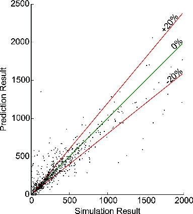
First, neither kind of preprocessing improves the results. Secondly, when comparing the remaining 3 models, kriging produces the best results on the training data, whereas LOLIMOT is worst. However, when looking at the test results, kriging shows a significant reduction in prediction quality compared to the training results, whereas LOLIMOT and SVR show robust behavior. Setting the mean average errors of 87 and 84 (LOLIMOT noPCA, SVR noPCA) in relation to the upper limit taken into account by the EuroNCAP assessment protocol (1,700)<A gives a relative mean error of 5% for the predicted values. An exemplary comparison of the FEA simulation and the LOLIMOT prediction values can be found in Figure 5.

Leg Impact Results

For the leg, 3 criteria (acceleration, bend, and shear) and 3 methods for selection of training data sets have to be looked at. Generally, the changes from training to test data are larger than for the head impact models. In addition, neither kind of preprocessing improves the results in most cases and is not considered any further.

Looking at the training data selection method, the model prediction quality shows no clear evidence for one of the methods. For the relative change in model prediction quality, the LHS training data set selection variants show the least change for all 3 injury criteria. In particular, SVR with LHS training data selection has the best performance for acceleration and bending and second best for shear (the best here is LOLIMOT using LHS). However, these 2 variants are also the ones with the largest error on the training data.

Looking at the different model types, kriging is best when looking at the model prediction quality but worst at the relative change, whereas LOLIMOT is best concerning relative change and second in model prediction quality.

Due to these results, no definitive decisions can be made about the best data set selection method and the best model to use. However, setting the worst mean average errors of the remaining 9 data set/model combinations in relation to the upper limits taken into account by the EuroNCAP assessment protocol (200 g for leg acceleration, 20° for leg bending, and 7mm for leg shear) gives a relative error of 12% for leg acceleration, 17% for leg bending, and 6% for leg shear.

The LOLIMOT and SVR models show good performance for the head impact, whereas kriging seems to overfit the training data. For the leg no clear favorite could be found but the relative errors found were all below 18% of the upper EuroNCAP limits.

Application Example

The models, once trained, can be used as replacement for complex but slow FEA models in large-scale studies, allowing injury-based effectiveness assessment of active, passive, and integrated safety systems as shown in Ferenczi et al. (2014), where a simulation method to assess the effectiveness of integrated pedestrian protection systems using the surrogate models is described. First, a stochastic traffic simulation was used to simulate 1 million scenarios where a pedestrian tries to cross a traffic stream. If a scenario leads to a collision between a car and the pedestrian, a more detailed multibody system model was used to determine the leg and head impact location and velocity. This was the case in 1,000–2,000 cases depending on whether an automatic emergency brake system was used or not. Surrogate models for the leg impact on the bumper and for the head impact on a conventional and an active hood were used to determine the resulting injury criteria values based on the impact constellations. These injury criteria values were then used to assess the overall effectiveness of the automatic emergency brake system, the active hood, and the combination of both systems in comparison to a vehicle without those systems.

Limitations

Because the surrogate models are specific to a certain vehicle, training has to be redone for a new vehicle. Still, there is a large benefit regarding calculation time when doing large-scale studies: Whereas a typical calculation time for the FEA calculation is several hours on a computer cluster system, the training of a surrogate model takes about one hour on a desktop PC and the calculation time of the trained surrogate model is less than one second for about 1,000 data sets.

Despite the use of cross-validation during training, some, but not all, models show significant overfitting. This complicates the decision regarding which model to choose when no large amount of additional test data is available as would be the case during a vehicle development process.

Outlook

The method itself can also be applied to approximate other injury criteria or be used in different accident scenarios.

Further investigations will include studying the influence of the amount and distribution of training data on prediction error and robustness. In addition, the method will be applied in the analysis of cyclist accidents.

Funding

VIRTUAL VEHICLE Research Center is funded within the COMET (Competence Centers for Excellent Technologies) programme by the Austrian Federal Ministry for Transport, Innovation and Technology (BMVIT), the Federal Ministry of Science, Research and Economy (BMWFW), the Austrian Research Promotion Agency (FFG), the province of Styria, and the Styrian Business Promotion Agency (SFG). The COMET programme is administrated by FFG.

We would furthermore like to express our thanks to our supporting industrial and scientific project partners, namely, BMW Group and the Graz University of Technology.

Supplemental Materials

Supplemental data for this article can be accessed on the publisher's website