Combining Coordination of Motion Actuators with Driver Steering Interaction

Abstract

Objective: A new method is suggested for coordination of vehicle motion actuators; where driver feedback and capabilities become natural elements in the prioritization.

Methods: The method is using a weighted least squares control allocation formulation, where driver characteristics can be added as virtual force constraints. The approach is in particular suitable for heavy commercial vehicles that in general are over actuated. The method is applied, in a specific use case, by running a simulation of a truck applying automatic braking on a split friction surface. Here the required driver steering angle, to maintain the intended direction, is limited by a constant threshold. This constant is automatically accounted for when balancing actuator usage in the method.

Results: Simulation results show that the actual required driver steering angle can be expected to match the set constant well. Furthermore, the stopping distance is very much affected by this set capability of the driver to handle the lateral disturbance, as expected.

Conclusion: In general the capability of the driver to handle disturbances should be estimated in real-time, considering driver mental state. By using the method it will then be possible to estimate e.g. stopping distance implied from this. The setup has the potential of even shortening the stopping distance, when the driver is estimated as active, this compared to currently available systems. The approach is feasible for real-time applications and requires only measurable vehicle quantities for parameterization. Examples of other suitable applications in scope of the method would be electronic stability control, lateral stability control at launch and optimal cornering arbitration.

Keywords:

• driver interaction
• control allocation
• actuator coordination
• split friction
• heavy commercial vehicles
• AEBS

Introduction

Human drivers can effectively adapt and assess new situations. Computer-controlled vehicles can do boring things millions of times in a reliable and quick way. A combination of these 2 is therefore appealing when striving for safe vehicles. Systems developed to assist the driver, traditionally known as advanced driver assistance systems (ADAS), are often developed to support the driver in only one specific direction: longitudinal, lateral, roll, etc. An advanced emergency braking system (AEBS), controls the longitudinal motion to avoid collision by braking. Another example is electronic stability control (ESC), often with the primary objective of controlling vehicle yaw motion. Because motions are coupled, other directions can be affected. An example is that AEBS, which is soon mandatory on heavy trucks in Europe (European Union 2012), may cause lateral deviation when activated on a split friction road segment (Tagesson et al. 2014). Here, the driver needs to actively steer to reduce this lateral drift induced by uneven brake action. Another example is braking-based ESC, which causes speed to decrease; this might be undesirable when traveling uphill. When affecting motions in other directions than the primary one, it is important to balance the assistance to guarantee safety. In this article we look at how to handle and limit such disturbances induced via coupled motions, using a generic approach that is different from previously known methods. We only consider vehicles with a mechanical connection between driver steering interface and front wheels. The methods developed are in particular suitable for heavy commercial vehicles or heavy vehicle combinations. In general, these have more actuators than controlled motions. This implies that actuator coordination is needed. Previous research has suggested control allocation (CA), methods as a structured way of including a variety of motion actuators to coordinate for the desired motion of the vehicle or even articulated vehicle combination (Tagesson et al. 2009; Tjønnås and Johansen 2010; Uhlén et al. 2014). CA makes it possible to achieve a modularized control architecture, where high-level control modules determine the control objective of the motion and lower level modules allocate forces among actuators. The methods are feasible in real time (Tagesson et al. 2009) and can be extended to a model predictive control formulation in order to include actuator dynamics (Luo et al. 2007).

Manning and Crolla (2007) summarized state-of-the-art methods for lateral control of passenger vehicles. More or less all methods work according to the following principle, determine what the intention of the driver is and then control the vehicle such that this is achieved, while maintaining stability. The same principle can be observed for available CA applications, as in Doumiati et al. (2011), Knobel (2009), and Tjønnås and Johansen (2010). For modern vehicles equipped with ADAS systems the situation is somewhat different. It is not only the intention of the driver that triggers controls, for example, AEBS can trigger heavy deceleration in order to avoid collision. If this action causes disturbances via coupled motions, we can consequently not rely on the driver only, unless we limit these disturbances to a safe level. A connection between driver and motion coordination is missing. No publication has been found proposing how to represent this link. The objective here is to develop a method for this, where motion actuators are coordinated to maximize the maneuverability and stability of the truck and where driver feedback and capabilities become natural elements. This is the focus of this article.

On current commercial road vehicles the problems involved with coupled motions are most often handled in a nongeneric way. Constraints are, for instance, implemented at the actuator level, making it impractical once vehicle configuration changes. Therefore, the method developed should also preferably adapt to changing vehicle, road, or driver conditions. What this means becomes clearer when looking at an example of how brakes are configured on current commercial vehicles during split-friction braking. A simple rule is introduced per axle, allowing only a fixed amount of deviation in brake pressure between left and right side of the axle. In Kharrazi et al. (2008), the yaw velocity was measured and used to control the rear-axle steer angle of a truck during split-friction braking on a test track. When the conventional axle brake-limiting functionality was relaxed it was seen that a 10% shorter stopping distance was achieved, while maintaining the required driver steering profile from a conventional truck. It is, however, clear that with this approach it is hard to calculate how much the brake pressure should be allowed to differ between the sides of a single axle. Once all actuators affecting the motion of the vehicle are coordinated jointly it becomes easier; this is why CA is a good starting point.

The article is structured as follows. First the generic principle of the method is described. This is followed by simulations of the scenario AEBS activated on a split friction road to exemplify the usage of the method. A final discussion concludes the findings and the results. Sign conventions used are compliant with ISO 8855 (International Organization for Standardization [ISO] 2011). Units are SI unless otherwise stated.

Methods

An important starting point for CA is that the equations of motions for the vehicle can be approximated with an affine state space form (1)

with a k-dimensional state vector x including, for example, longitudinal speed, lateral speed, and yaw velocity. Furthermore, g and h are general functions, and the m-dimensional actuator vector u is composed of, for example, brake torque, engine torque, and rear-axle steering angles. If a sufficiently short time interval is considered it further holds that h(x)u ≈ Bu, with B ∈ ℜ^{k × m}, known as the control effectiveness matrix. The basics in CA is to achieve where v is known as the virtual control vector. For road vehicle planar motion control, v is preferably composed from resulting longitudinal force F_x, resulting lateral force F_y, yaw torque M_z, and possible trailer counterparts (Uhlén et al. 2014). (2)

After having made the substitution from actuator-dependent properties to a virtual control vector, the problem is decoupled. Firstly, a motion control part considering the system . Secondly, a control allocation part trying to achieve Bu = v and thus making the residual Bu − v = 0. Because u is constrained, the latter is not always possible. The residual then becomes a measure of the infeasibility in the virtual control request. Because v normally is a selection of resulting forces and torques that counteract, it is sometimes possible to constrain the residual according to (3) where v_min and v_max are vectors of size k. These can both be used in the motion control part to limit disturbances via coupled motions, as will be explained more in detail below.

The decoupling achieved is visualized graphically in Fig. 1, where the main architecture of the developed method is shown. There are three layers:

1. The vehicle motion control layer deriving desired total vehicle forces and torques, thus composing v. Also, as suggested in Eq. (3(3) ), including v_min and v_max to limit allowed deviation from v.

2. The control allocation layer that coordinates all actuators, resulting in u.

3. Finally, the actuator control layer, which is represented for each actuator i, serving as a slave controller to the reference u_i and also providing estimates of actuator limitations u_{min, i} and u_{max, i}.

Fig. 1. The control architecture has a decoupled control strategy where actuators are grouped into resulting vehicle forces and torques, v, above the control allocation layer. The vector u is generally composed from a mix of quantities, typically shaft torques on wheels, brake torque on wheels, and steering angles of axles. Double-line arrows indicate vector signals and single-line arrows scalar signals.

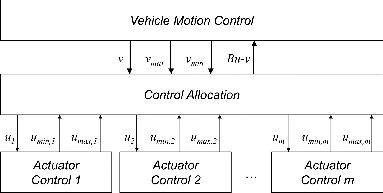
These layers will now be explained in more detail starting from the bottom and up. As mentioned previously, an implementation of AEBS will be used to exemplify the usage of the method. It is setup for a 6 × 2 rigid truck having one brake actuator per wheel. Figure 2 shows a more detailed version of the main architecture as used in this AEBS example. The details will be explained along with the example.

Fig. 2. Control architecture as used in the AEBS example.

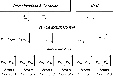
Actuator Control

For each actuator included in the controls there is a function handling local control of the actuator. Both range estimation and error-controlled regulation should be included.

As seen in Fig. 2, 6 brake actuators are used in the AEBS implementation. A longitudinal force request, F_xri = u_i, is input to the actuator belonging to wheel i. In the remainder the index i = {1, 2, 3, 4, 5, 6} denotes, in order, front left, front right, drive (first rear axle) left, drive right, tag (second rear axle) left, or tag right. This request is simply multiplied by the effective wheel radius R_e to form the resulting wheel torque. The effective wheel radius can be estimated from a free rolling wheel as R_e = v_x/ω_wi, where v_x is vehicle longitudinal speed, and ω_wi is wheel speed. To avoid excessive wheel slip a scale factor f_i is used according to (4) (5)

where v_xi is wheel longitudinal speed and T_i is wheel torque, which is applied directly to the wheel. The value 0.1 reflects peak friction slip level.

Friction is assumed known when estimating the brake force range according to (6) where μ_i is the current friction level at wheel i and F_{z, i} is the current vertical force at wheel i. The maximum brake force u_{max, i} is set to 0. This makes the actuator capability vector F_xci = [ − μ_iF_{z, i}, 0].

Control Allocation

There is in general no guarantee for an existing u to fulfill Eq. (2(2) ). When no solution exists, some arbitration rule has to be applied. In CA a common way is to minimize the weighted norm ‖W_v(Bu − v)‖₂, specifically, the ℓ₂-norm, for alternatives see Laine (2007). On the other hand, if the solution is not unique as dim(v) < dim(u), some secondary rule has to be introduced to achieve uniqueness. By using a weighted ℓ₂-norm for this the weighted least squares problem for CA can be formulated as (7) where W_u and W_v are weighting matrices, u_d is a desired set point of the actuator vector u, and γ is a high scalar weight to emphasize the importance of achieving a small residual. More details about this formulation can be found in Härkegård (2003).

In particular, the W_v matrix can be used to emphasize what force or torque in v that is of highest importance to fulfill. All other terms will be subordinate. This can make the traditional formulation of CA, as in Eq. (7(7) ), hard to use in practice. A particular element in v can often be prioritized; however, all other elements cannot be fully subordinate; that is, released. Getting back to the AEBS implementation running on split friction, it is clear that deceleration is prioritized, but the induced yaw torque must be limited. As previously suggested in Eq. (3(3) ), this can be achieved by adding extra constraints according to

With this formulation it is possible to prioritize a specific element in v, using W_v, at the same time as limitations are put on other elements using v_min and v_max. The choice of v_min and v_max must, however, be made with some caution in order to make sure that the feasible set is non-empty. In the AEBS example this is guaranteed because u_min ⩽ 0 ⩽ u_max and v_min ⩽ 0 ⩽ v_max. Thus, a trivial solution exists and guarantees a non-empty feasible region. In a more general case there is no explicit way of showing this property; there are, however, iterative methods for this; for example, simplex phase I (Nocedal and Wright 2006).

An Active Set solver, implemented in MATLAB m-code, was developed for solving Eq. (8). The solver will be uploaded to Matlab Central File Exchange for public access. It is marked with hashtag #tagessonwlssolver. The solver was run on a dSpace Micro Autobox II to test real-time feasibility. The worst-case turnaround time observed for producing a solution was 0.15 ms. This can be compared to 0.06 ms, which was achieved in a similar setup when using a C version Active Set solver for solving Eq. (7(7) ) in Tagesson et al. (2009). It is common for vehicle motion control systems like ESC and AEBS to run at ∼ 10 ms. The method is consequently feasible in real time.

In the AEBS implementation the virtual control vector used is where F_{x, req} is the desired resulting longitudinal force and M_{z, req} is the desired resulting yaw torque. We assume small slip angles of wheels and no combined slip relation in the allocation. This makes the control effectiveness matrix become where w_f, w_d, and w_t are vehicle track width on the front, drive, and tag axle, respectively. The weighting matrices used are as suggested in Tagesson et al. (2009). The units of W_v is diag[1/N, 1/Nm] and for W_u all elements have the unit 1/N. All other CA parameters used in the implementation of Eq. (8) can be found in Tables 1 and 2.

Table 1. Specification of 6 × 2 truck vehicle model. The axles are referred to in order as front, drive, and tag, meaning first, second, and third

Property	Value	Unit	Description
m	25,460	kg	Vehicle mass
L	4.8	m	Wheelbase, distance between front and drive axle
bs	1.37	m	Boogie spread, distance between drive axle and tag axle
hcog	1.66	m	Sprung body center of gravity height
Fz, f	71,220	N	Front axle vertical load at standstill
Fz, d	118,111	N	Drive axle vertical load at standstill
Fz, t	60,430	N	Tag axle vertical load at standstill
is	23		Steering ratio, road wheel angle to Steering Wheel angle
R	0.5	m	Wheel radius
wf	2.05	m	Front axle track width
wd	1.85	m	Drive axle track width
wt	2.05	m	Tag axle track width

Table 2. Controller specific parameters used in the AEBS implementation

Property	Value	Unit	Description
g	9.81	kg	Vehicle mass
γ	100		CA weight
ud	[0, 0, 0, 0, 0, 0]^⊺	N	Actuator set-point
Kas	8.47 × 10^4	Nm/rad	Anti steer gain
Re	0.525	m	Effective wheel
			radius

Vehicle Motion Control

There are many tasks that a motion controller can be used for. As seen in Manning and Crolla (2007), it is a subject on its own. The important aspect to be stressed here is depicted in Fig. 1. The motion controller should not only control the primal motion of interest but should also limit other degrees of freedom that can be affected. This can be done using v_max and v_min.

In Fig. 1 one arrow indicates the residual Bu − v as propagated to the motion control layer. This information can be used for supporting the driver in negotiating induced coupled forces, for instance, by adding a supporting torque T_as onto the steering wheel. This is, however, not used in the simulations that follow.

In the AEBS implementation the motion control layer (see Fig. 2), receives a request of longitudinal acceleration a_{x, req} from AEBS logics located on the ADAS layer. This request is simply multiplied with the vehicle mass m to form F_{x, req}; that is, an open-loop acceleration controller. When braking it is not desirable to induce yaw torque; hence, M_{z, req} = 0 is used. If, however, yaw torque is induced anyway this should be limited according to what the driver can handle. Assuming that the driver is able to produce a steering wheel angle, δ_d, equal to a set value δ_as, where the index as denotes anti-steer, it is possible to estimate how much yaw torque the driver can reach. A simple way is to use a steady-state planar linear vehicle model. It can easily be shown that an applied yaw torque is cancelled out from steering when where c_f is effective front cornering stiffness, c_r is effective rear cornering stiffness, l_f and l_r are the distances from vehicle center of gravity to front axle (respectively rear axle), and i_s is steering gear ratio. As seen, it is possible to group parameters and define a constant parameter K_as that can be tuned for a specific vehicle. Using this model and assuming that the driver can steer at most ± δ_as it is possible to limit the induced yaw torque error by where we chose to keep the first entry, due to longitudinal force error, unlimited.

Results

A series of simulations was performed including a high-fidelity truck model, developed by Volvo, and the implementation of the AEBS structure as presented. The simulations were run under split-friction conditions on a straight road. The purpose of the simulations was to test whether the method really is capable of performing actuator coordination so that the value of δ_as effectively limits how much steering that is expected from the driver and where this is performed under more realistic circumstances.

Simulation Setup

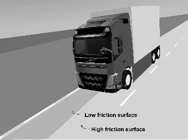
The high-fidelity truck model is shown in Fig. 3. It includes, for example, magic tire formula tire model with relaxation, frame twist, suspension, and rotating wheels and has been validated extensively. The main parameters of the model are shown in Table 1. Peak friction, μ, was set to 1.0 under the left side wheels and 0.2 under the right side wheels. The model and all other parts in the simulations were run in MATLAB Simulink.

Fig. 3. A 6 × 2 truck model was used in the simulations for the AEBS implementation running on split friction.

A proportional–integral–derivative (PID) controller was used to control the steering wheel angle. The target of the controller was to keep the vehicle’s center of gravity lateral position, Y, as low as possible. This was also the only input to the controller. The proportional gain was 1.1 rad/m, the integral gain was 0.44 rad/(m·s), and the derivative gain was 0.22 rad·s/m. With this setup it was possible to determine how much steering that is required to fully remove a yawing torque.

AEBS braking was activated after one second, where a_{x, req} was ramped down to − 6 m/s² after first passing a first-order low-pass filter taking account of actuator dynamics, with time constant 0.1 s. Allowed yaw torque was varied by altering anti-steer level according to δ_as = {10°, 20°, 40°, 60°}. The initial speed was set to 22.2 m/s (80 km/h). To avoid numerical problems, a_{x, req} was ramped down to zero, using the same filter as for ramp-up, when the speed dropped below 4 m/s (14.4 km/h).

Simulation Results

Figures 4 and 5 show how the implementation performs in simulation. First of all, the longitudinal speed is shown in Fig. 4. As can be seen, the speed drop is heavily influenced as the allowed yaw torque is altered. Looking at the longitudinal acceleration, shown in the second subfigure of Fig. 4, the same trends can be seen. The request a_{x, req} = −6 m/s² is never reached. The δ_as = 60° line is close to − 5 m/s², which is almost as low as what is possible to ever achieve considering friction level and load transfer. Obviously the vehicle motion control layer is requesting more than what is possible to achieve in all of the different cases.

Fig. 4. Results from simulations of the AEBS example run on split friction. The subfigures show, in order, longitudinal speed, v_x, longitudinal acceleration, a_x, and steering wheel angle, δ_d. The required steering action by the driver agrees roughly with what has been configured as δ_as.

Fig. 5. Additional time series corresponding to the same simulations as shown in Fig. 4. The subfigures show, in order, lateral deviation, Y, longitudinal force residual, F_x − F_{x, req}, and yaw torque residual, M_z − M_{z, req}. As can be seen, the error in longitudinal force is highly linked to the set limit of yaw torque.

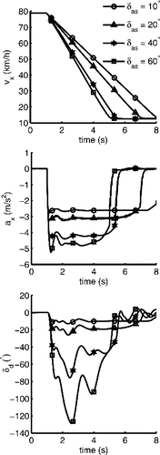
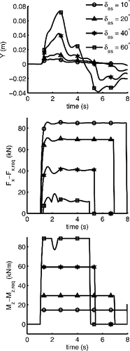
The steering profile performed by the PID controller is shown in the last subfigure of Fig. 4. It can be seen that the steering wheel angle, δ_d, is close to the programmed limit δ_as in steady state. There are some oscillations, but the overall profile is close to δ_as. The first subfigure in Fig. 5 shows the lateral deviation. As can be seen, it is held at a low level, meaning that the PID steering controller works as intended; it represents an ideal driver. And this ideal driver only needs to work with steering wheel angles around the programmed limit δ_as. The two bottom subfigures in Fig. 5 together show the residual resulting from CA; that is, the difference between the requested and allocated longitudinal force and yaw torque respectively. As can be seen, M_z is limited by v_max almost constantly, whereas F_x − F_{x, req} is lowered as more yaw torque is allowed.

Furthermore, Figs. 4 and 5 clearly show that the stopping distance is and should be linked to the estimated capacity of the driver to actively adjust for a disturbance. For instance, when comparing the two settings δ_as = 60° and δ_as = 10° the stopping distance increases by 80%. Consequently, if brakes are the only actuators involved, this also corresponds to how much adaptation that is necessary in order to handle a fully passive driver and a more active driver when no lateral deviation can be accepted.

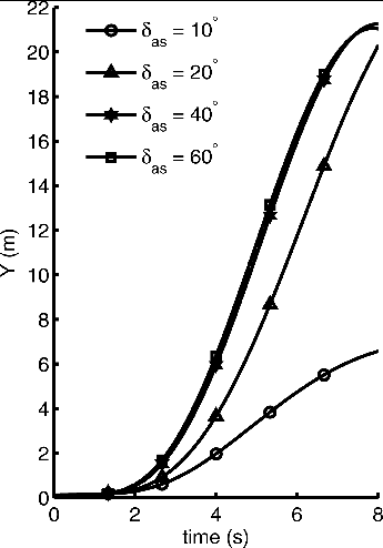
To underline the severity of the scenario, yet another simulation was run where no steering was performed. The lateral position can be seen in Fig. 6. The two cases δ_as = 40° and δ_as = 60° both end up at 90° sideslip and a lateral deviation of more than 20 m. In the other two cases, δ_as = 10° and δ_as = 20°, the lateral deviation is reduced and both end up heading forwards.

Fig. 6. Lateral position shown when no steering action is performed.

Discussion

As clearly shown by simulation, it is possible to induce severe disturbances in secondary vehicle states when conditions are imperfect. Because the driver is supposed to handle these disturbances it is important to estimate the driver's ability to do so and thereafter balance the coordination among actuators. We present an extended control allocation method where motion actuators are coordinated in accordance to what is requested and available and where driver feedback and capabilities become natural elements. The capability of the driver to handle a yaw disturbance in the AEBS use case was expressed in terms of the required maximum driver steering wheel angle. The simulation results show that this limit actually was roughly achieved. In other vehicle control approaches, as seen in, for example, Manning and Crolla (2007), this natural way of taking account of driver capabilities is not seen. For brake systems in heavy vehicles the difficulties in split friction are handled by an axle brake-limiting approach, which cannot account for dynamic driver characteristics. This new setup has the potential of shortening the stopping distance when the driver is estimated as active. In addition when using the suggested method, it is beneficial to constantly estimate the capability of the driver to handle disturbances. In the AEBS case, for instance, this will have a direct connection to the stopping distance, which preferably should be accounted for in the higher level decision-making layer, triggering AEBS activation.

Another benefit of the method is that it is independent on vehicle configuration, meaning that it is possible to derive settings from physical properties and dimensions. The set of actuators being used can easily be extended to coordinate not only brake actuators but also rear axle steering, which is common on heavy vehicles. The method was also shown to be suitable for real-time usage.

In the simulations, the method was configured as an open-loop controller, meaning that neither longitudinal nor yaw states were fed back into the controller during the maneuver. This will make it sensitive to errors in the models of actuators, in particular to estimates of road-to-wheel friction. In a real implementation of the method, where this knowledge is not as easy to obtain, this needs to be considered and accounted for in some way, for example, by feeding back more states as in Tagesson et al. (2009). Another limitation of the suggested method lies in that the CA formulation used only considers infinitely fast actuators. This is obviously not true. When including coordination of steering this will become more obvious because the rate constrains of the involved actuators are different. Here state feedback could again prove useful. Another suggestion would be to use a time horizon, as in Luo et al. (2007).

For future work we suggest a more realistic assumption about the knowledge of friction. We also stress the possibility of guiding the driver using steering wheel torque by means of the residual calculated in the allocation step. Furthermore, when involving more actuators, like steering and power-train, the actuator dynamics will prove more important to account for. Also central in the method is a good understanding of driver capacity. Exactly how this should be done provides a research field of its own. Other possible applications of the method, apart from AEBS, would be electronic stability control, lateral stability control at launch, and optimal cornering arbitration.

References

- Doumiati M, Sename O, Martinez JJ, Dugard L, Gaspar P, Szabo Z, Bokor J. Vehicle yaw control via coordinated use of steering/braking systems. Paper presented at: 18th IFAC World Congress (IFAC WC 2011); August 28–September 2, 2011; Milan, Italy.
- European Union. Commission regulation (EU) No. 347/2012 of 16 April 2012. Official Journal of the European Union. 2012;109:117.
- Härkegård O. Backstepping and Control Allocation with Application to Flight Control. Linköping, Sweden: Linköping University, Department of Electrical Engineering; 2003.
- International Organization for Standardization. International Standard 8855, Road Vehicles and Road Holding Ability—Vocabulary. ISO. 2011.
- Kharrazi S, Lidberg M, Lingman P, Svensson JI, Dela N. The effectiveness of rear axle steering on the yaw stability and responsiveness of a heavy truck. Veh System Dyn. 2008;46:365–372.
- Knobel C. Optimal Control Allocation for Road Vehicle Dynamics Using Wheel Steer Angles, Brake/Drive Torques, Wheel Loads and Camber Angles. Munich,Germany: Institut für Robotiks und Mechatronik, Deutsches Zentrum für Luft- und Raumfahrt; 2009.
- Laine L. Reconfigurable Motion Control Systems for Over-actuated Road Vehicles. Göteborg, Sweden: Chalmers University of Technology, Department of Applied Mechanics; 2007.
- Luo Y, Serrani A, Yurkovich S. Model-predictive dynamic control allocation scheme for reentry vehicles. J Guid Control Dyn. 2007;30:100–113.
- Manning W, Crolla D. A review of yaw rate and sideslip controllers for passenger vehicles. Trans Inst Meas Control. 2007;29:117–135.
- Nocedal J, Wright SJ. Numerical Optimization. 2nd ed. New York: Springer; 2006.
- Tagesson K, Jacobson B, Laine L. Driver response to automatic braking under split friction conditions. Paper presented at: 12th International Symposium on Advanced Vehicle Control (AVEC14); September 22–26, 2014; Tokyo, Japan.
- Tagesson K, Sundström P, Laine L, Dela N. Real-time performance of control allocation for actuator coordination in heavy vehicles. Paper presented at: IEEE Intelligent Vehicles Symposium (IV); June 3–5, 2009; Xian, China.
- Tjønnås J, Johansen TA. Stabilization of automotive vehicles using active steering and adaptive brake control allocation. IEEE Trans Control Syst Technol. 2010;18:545–558.
- Uhlén K, Nyman P, Eklöv J, Laine L, Sadeghi Kati M, Fredriksson J. Coordination of actuators for an A-double heavy vehicle combination. Paper presented at: 17th International IEEE Conference on Intelligent Transportation Systems, October 8–11, 2014; Quingdao, China.