Toward harmonizing prospective effectiveness assessment for road safety: Comparing tools in standard test case simulations

Abstract

Objective: With the overall goal to harmonize prospective effectiveness assessment of active safety systems, the specific objective of this study is to identify and evaluate sources of variation in virtual precrash simulations and to suggest topics for harmonization resulting in increased comparability and thus trustworthiness of virtual simulation-based prospective effectiveness assessment.

Methods: A round-robin assessment of the effectiveness of advanced driver assistance systems was performed using an array of state-of-the-art virtual simulation tools on a set of standard test cases. The results were analyzed to examine reasons for deviations in order to identify and assess aspects that need to be harmonized and standardized. Deviations between results calculated by independent engineering teams using their own tools should be minimized if the research question is precisely formulated regarding input data, models, and postprocessing steps.

Results: Two groups of sources of variations were identified; one group (mostly related to the implementation of the system under test) can be eliminated by using a more accurately formulated research question, whereas the other group highlights further harmonization needs because it addresses specific differences in simulation tool setups. Time-to-collision calculations, vehicle dynamics, especially braking behavior, and hit-point position specification were found to be the main sources of variation.

Conclusions: The study identified variations that can arise from the use of different simulation setups in assessment of the effectiveness of active safety systems. The research presented is a first of its kind and provides significant input to the overall goal of harmonization by identifying specific items for standardization. Future activities aim at further specification of methods for prospective assessments of the effectiveness of active safety, which will enhance comparability and trustworthiness in this kind of studies and thus contribute to increased traffic safety.

Keywords:

• Active safety
• driver assistance systems
• effectiveness assessment
• simulation
• harmonization

Introduction

Active safety and advanced driver assistance systems are developed and introduced into the automotive market every year. The question that arises is how the effectiveness of such systems in terms of crash avoidance and mitigation can be determined. Two types of methodologies exist in the field of safety assessment of the effectiveness of such systems: Retrospective methodologies use accident statistics. The application of these methodologies is limited by the time it takes for crash data to be collected (Kalra and Paddock 2016; Lindman et al. 2017) and the availability of information on accidents with and without such systems. Prospective methodologies predict effectiveness before market introduction (Alvarez et al. 2017; Page et al. 2015; Sander 2016) and are therefore used when market penetration rates are low or prior to market introduction.

Prospective effectiveness assessment of active safety systems typically includes complex interactions of the vehicle under test (VuT), its driver, the system under test (SuT), surrounding traffic, the environment, etc. A comprehensive assessment therefore requires a high number of test cases covering possible variations in interactions that influence crashes and criticality of situations. Virtual simulations are indispensable in such assessment because physical tests would be lengthy, expensive, and probably would not cover the necessary array of interactions.

An important aspect when using virtual simulation for such a task is the comparability of effectiveness studies performed by various stakeholders or research teams. For example, Kolk et al. (2016), Sander (2017), and Scanlon et al. (2017) presented studies on the effectiveness of intersection assistance systems. Comparing the presented systems’ effectiveness is not feasible, because the outcome of the studies depends not only on the differences in the systems but also on the simulation methodology used. The question therefore arises regarding which features of the simulation methodology need to be standardized to obtain comparable results and to what extent this harmonization is feasible.

This article presents a round-robin study of a well-specified problem set up by the P.E.A.R.S. initiative (Alvarez et al. 2017; Page et al. 2015) in order to make further progress toward harmonizing simulation methodologies. This study aims to identify typical aspects that have to be addressed in future prospective studies and how to reduce their influence on results in order to make them comparable.

The research question for this article is summarized as follows: Which aspects in the virtual simulation methodology cause differences in simulation results and need further harmonization when using different simulation tools in order to make the results comparable?

Method

A round-robin study was performed to identify aspects in virtual precrash simulations for prospective safety assessments. Input data, simulation model details, and simulation output analysis steps were specified. Eight different partners performed the study using their simulation tools and logic and the simulation output was analyzed, providing insight into the overall variations as well as most relevant sources for variation. One ideal autonomous emergency braking system that is capable of responding to interactions with cyclists (AEB-Cyclist), was chosen as the SuT for the round-robin study.

Input data

Input data describe the test cases in which the SuT was evaluated. Test cases were taken from the AEB-Cyclist testing system (Op den Camp et al. 2017) project, representing severe (in terms of resulting fatalities and severe injuries) passenger car–bicycle crash situations. In each test case, the car and cyclist are set to follow a straight line at constant speed, so that a collision at a prescribed location on both car and cycle would result in case AEB does not react. In total, there are 4 test cases (extended explanations can be found in the Appendix “Test Cases,” see online supplement):

• CVNB: Car-to–vulnerable road user (VRU) near-side bicyclist is a collision protocol in which a vehicle travels forward toward a bicyclist crossing its path cycling from the near side. The hit-point (lateral position of the bike’s crank shaft at time of collision) should lie at 50% of the vehicle’s width when no braking action is applied.

• CVNBO: Car-to-VRU near-side bicyclist obstructed is a collision protocol in which a vehicle travels forward toward a bicyclist crossing its path cycling from the near side from behind an obstruction. The hit-point should lie at 50% of the vehicle’s width when no braking action is applied.

• CVFB: Car-to-VRU far-side bicyclist is a collision protocol in which a vehicle travels forward toward a bicyclist crossing its path cycling from the far side. The hit-point should lie at 25% of the vehicle’s width from the far side when no braking action is applied.

• CVLB: Car-to-VRU longitudinal bicyclist is a collision protocol in which a vehicle travels forward toward a bicyclist cycling in the same direction in front of the vehicle. The hit-point should lie at 50% of the vehicle’s width when no braking action is applied.

Simulation tools

Because the study aims to assess differences in simulation tools for prospective effectiveness assessment, the tools selected by each contributing partner were used. Table A2 (see online supplement) highlights the essential characteristics of the different tools; additional information can be found in Appendix Part B–Simulation Tool Details (see online supplement).

Simulation models

AEB-Cyclist, considered in the European New Car Assessment Programme (Euro NCAP) safety assessment (Euro NCAP 2017) since January 2018, was chosen as an example SuT. The ideal AEB-Cyclist model used here consists of a sensor, control algorithm, and braking actuator.

The ideal sensor model is described by its position and alignment on the car and its field of view (FoV) with parameters opening angle and range. Three setups, differing only by their opening angle, were used. They are referred to as “small” (opening angle: 48°), “medium” (60°) and “large” (90°) FoV. These different setups refer to different levels of state-of-the-art sensor systems: Small refers to 2016 state-of-the-art production sensors, medium to the expected state-of-the-art in 2018 when the Euro NCAP protocol is introduced, and large to beyond state-of-the-art systems.

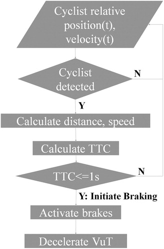
The control algorithm consists of 2 steps: First, the complete cyclist’s surface must overlap with the sensor’s FoV to be considered detected. This condition must remain valid for a certain duration (classification delay) for the cyclist to be identified. The algorithm fires and initiates braking if the time-to-collision (TTC) drops below a set threshold of 1 s after cyclist classification.

Automated braking starts after a set additional actuator delay of 0.2 s. The maximum deceleration was set to 0.9 g, to be reached linearly over a buildup time of 0.36 s. The study only considers automated braking; driver warning and driver response are outside the scope of the current study. Further details are given in the Appendix (“Ideal AEB Model,” see online supplement).

No specifications were given for vehicle and bicycle dynamics models because they are core models of the simulation tools under test.

To simulate the collision between a vehicle and cyclist, the geometry of the vehicle front and the cyclist–bicycle combination were specified. A generic 2D VuT shape was used, 4.5 m in length and 1.9 m in width. Its rounded front is linearly approximated by a 6-point polyline (see Appendix “Geometry of the Car,” Figure A2, online supplement). Bicycle and rider shapes were simplified into a 2D object composed of 3 rectangles, totaling 1.95 m in length and 0.5 m in maximal width (see Appendix “Geometry of the Cyclist,” Figure A3, online supplement).

Simulation output analysis

A postprocessing workflow was defined to analyze the results. This analysis consists of 3 steps, in order to identify aspects of the simulation methodology that impact the estimated effectiveness:

1. Discrete value analysis on time-independent results such as collision speed or collision avoidance (yes/no).

2. Time evolution–based analysis evaluating time-dependent values such as position, speed, and deceleration profiles for the complete duration of the test.

3. Flow of actions–based analysis, a detailed analysis focusing on individual test cases where significant states before the crash are recorded and compared for each simulation tool.

Discrete values analysis

All test cases (CVNB, CVNBO, CVFB, and CVLB) are used for discrete values analysis. Bicycle speeds are not varied in the same test case, but VuT speed is increased from 20 to 60 km/h, by steps of 5 km/h. All 3 sensor setups are also used for each test case. This results in 102 simulated configurations (4 test cases with [3 × 9 + 1 × 7] VuT speed steps × 3 sensor setups). For each of these configurations, the following discrete values were computed:

1. VuT collision speed: In cases where a collision is avoided, whether the VuT stopped before crossing the cyclist’s path or whether the VuT and cyclist crossed each other’s path without a collision is reported.

2. VuT speed reduction (initial speed − final speed): In case of a collision, the final speed difference between the vehicle and the bicycle in the vehicle driving direction is considered to be the impact speed. In other cases, the VuT speed is either zero (the VuT has come to a complete stop) or the VuT speed when crossing the bicycle’s trajectory is taken.

3. TTC at time of cyclist detection.

4. TTC at time of AEB system firing.

Based on these discrete values, binary (true/false) events such as “cyclist detected,” “algorithm fired,” and “collision avoided” were determined.

For each of these events, a conformity rate, defined as (1) $$\frac{n_{\text{cases with identical result for all participants }\left(\text{all true or all false}\right)}}{n_{\text{all testcases}}},$$(1) is calculated. Because no reference values for those events exist, it is impossible to use them as ratings for individual tools. They are instead used to quantify result variability between tools. Furthermore, for each tool and for each sensor setup, the following values were calculated to learn about the overall variation in the results: (2) $$\text{Cyclist detection rate}:\mathrm{ }\frac{n_{\text{cases cyclist detected}}}{n_{\text{all testcases}}}$$(2) (3) $$\text{Algorithm firing rate}:\mathrm{ }\frac{n_{\text{cases algorithm fired}}}{n_{\text{all testcases}}}$$(3) (4) $$\text{Collision avoidance rate}:\mathrm{ }\frac{n_{\text{cases collision avoided}}}{n_{\text{all testcases}}}$$(4)

(5) $$\text{Average speed reduction}:\mathrm{ }\frac{1}{n_{\text{all testcases with collision}}}\sum _{i=1}^{n_{\text{all testcases with collision}}}{(v}_{\mathrm{initial}}-v_{\mathrm{collision}}).$$(5)

Time evolution–based analysis

The results of the discrete value analysis can only quantify the overall variation in results and are not suitable for learning more about the reasons for these variations. Therefore, the time evolution of the variables was investigated in more detail for the complete duration of 2 configurations:

• “CVNB60small”: CVNB test case, initial VuT speed of 60 km/h, small sensor opening angle (48°), with and without AEB.

• “CVFB50medium”: CVFB test case, initial VuT speed of 50 km/h, medium sensor opening angle (60°), with and without AEB.

Flow of actions–based analysis

A more detailed analysis was carried out based on the flow of actions (Figure 1) to identify sources of variation and possible targets for further harmonization. This analysis starts at the final action “decelerate VuT” and moves backwards to the flow direction continuing with “activate brakes” and “initiate braking,” “calculate TTC” until the action “calculate distance, speed.” Cyclist detection was not analyzed further for the 2 configurations because the cyclist was detected by all partners much earlier than TTC = 1 s. The analysis aims to quantify time ranges for each action step where possible.

Figure 1. Simplified flow diagram of the investigated safety system.

Results

The results of 8 partners who conducted the round-robin study are presented in relation to the 3 analysis steps described in the Method section.

Discrete values analysis results

Values of the conformity rate for each sensor setup can be found in Table 1. Table 2 shows the minimum, maximum, mean, and median values as well as the range (maximum–minimum) of all participants for the cyclist detection rate (see Eq. (2)(2) $$\text{Cyclist detection rate}:\mathrm{ }\frac{n_{\text{cases cyclist detected}}}{n_{\text{all testcases}}}$$(2) ), the algorithm firing rate according to Eq. (3)(3) $$\text{Algorithm firing rate}:\mathrm{ }\frac{n_{\text{cases algorithm fired}}}{n_{\text{all testcases}}}$$(3) , collision avoidance rate Eq. (4)(4) $$\text{Collision avoidance rate}:\mathrm{ }\frac{n_{\text{cases collision avoided}}}{n_{\text{all testcases}}}$$(4) , and average speed reduction Eq. (5). More detailed results for each sensor setup can be found in Table A3 in Appendix Part C–Additional Result Plots and Tables of the Round-Robin Study (see online supplement).

Table 1. Percentage of test cases where all participants had same results (either true for all events cyclist detected, algorithm fired, and collision avoided).

Sensor setup	Detected (%)	Fired (%)	Avoided (%)
Sensor small FoV	44	44	38
Sensor medium FoV	65	65	29
Sensor large FoV	85	85	47

Table 2. Minimal, maximal, mean, median and range values of detection rate, firing rate, avoidance rate and average speed reduction for all sensor setups and participants.

Statistical value	Detection rate (%)	Firing rate (%)	Avoidance rate (%)	Average speed reduction (km/h)
Min	65	65	27	13.5
Max	100	100	64	22.7
Range	35	35	36	9.1
Mean	82	79	47	16.4
Median	78	77	48	14.9

Collision avoidance rates range from 15 to 56% for the small FoV sensor setup, from 24 to 65% for the medium FoV sensor setup, and from 44 to 74% for the large FoV sensor setup. Average speed reductions range from 7.9 to 17.8 km/h for the small FoV sensor setup, from 12.4 to 25.8 km/h for the medium FoV sensor setup, and from 19.7 to 26.4 km/h for the large FoV sensor setup.

Time evolution–based analysis results

For the CVNB60small and CVFB50medium configurations, all participants provided 1-ms sampled timelines for VuT position, speed and acceleration, cyclist position and speed, as well as sensor-measured distance to cyclist and TTC. Participants were free to set simulation starting times, which resulted in necessary postprocessing by the authors, so that t = 0 s at the time of collision for all participants.

The first step consisted in hit-point range investigation. The relevant value is the position of the cyclist at the time of collision in simulation runs without AEB. Deviations from correct hit-point range from −0.023 to +0.032 m for CVNB60small and from −0.043 to +0.064 m for CVFB50medium.

For the simulation runs with AEB, sensor and VuT data plots for time range from 1.3 s before collision until collision and can be found in Figures A6 and A7 (see online supplement). Once the estimated TTC is below 1 s, the time until the vehicles collide varies from 1.094 to 1.179 s (range of 0.085 s) for CVNB60small and from 1.163 to 1.362 s (range of 0.199 s) for CVFB50medium. The collision speeds show a variation from 34.3 to 37.8 km/h for CVBN60small and from 19.9 to 25.5 km/h for CVFB50medium.

Flow of actions–based analysis results

The results of the analysis for each action step described in Figure 1 are given in the following paragraphs. The complete list of result values can be found in Table 3.

Table 3. Minimal, maximal, and range (maximum-minimum) values of the results of the flow of actions–based analysis. “Firing” relates to the moment where TTC falls below the threshold.

Action step	Test case	Type of result	Min	Max	Range
Decelerate VuT	Brake test	Time to stop (s)	2.222	2.288	0.066
	CVNB60small	Speed reduction duration (s)	1.126	1.165	0.039
	CVFB50medium	Speed reduction duration (s)	1.208	1.247	0.039
Activate brakes	Both cases	Brake delay (s)	0.2	0.246	0.046
Initiate braking	CVNB60small	Offset theoretical–actual firing (s)	−0.013	+0.031	0.044
	CVFB50medium	Offset theoretical–actual firing (s)	−0.061	+0.02	0.081
Calculate distance, speed	CVNB60small	Distance at firing (m)	16.431	17.209	0.788
		v{VuT} at firing (m/s)	16.666	16.674	0.008
		v{cyclist} at firing (m/s)	4.165	4.167	0.002
	CVFB50medium	Distance at firing (m)	13.889	15.677	1.788
		v{VuT} at firing (m/s)	13.88	13.889	0.009
		v{cyclist} at firing (m/s)	5.555	5.556	0.001

• “Decelerate VuT”: As a presumed major source of variation, VuT model-dependent VuT braking behavior was analyzed first. Partners carried out a simple brake test simulation: Initial speed 60 km/h, braking at a prescribed time. Because the VuT cannot stop without a collision in CVNB60small or CVFB50medium, it is reasonable to analyze the variation in time to reach speed reduction (24.1 km/h for CVNB60small, 26.7 km/h for CVFB50medium) averaged over all participants at the time of collision instead of the time to stop. The variation in time to reach speed reduction has a range of 0.039 s for both CVNB60small and CVFB50medium.

• “Activate brakes”: The deceleration of the VuT starts with a delay after the TTC value falls below a threshold. This delay is caused by the cycle time of the algorithm and the brake system needing time to build up brake pressure, move the brake pads to the disc, etc. A respective delay value is included in the actuator definition (0.2 s before start of deceleration). The effective resulting delays are calculated for the 2 configurations with AEB as the time difference between the first moment where TTC ≤ 1 s and the first moment where a _{VuT} ≤ −0.01 m/s². The range for both configurations has an identical value of 0.046 s.

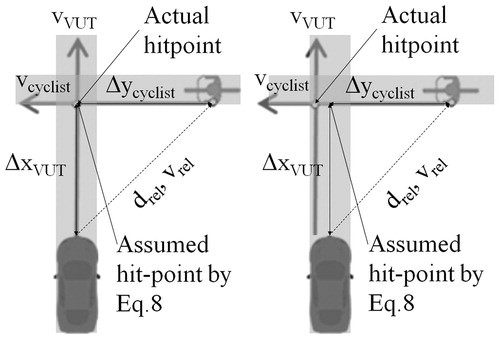
• “Initiate braking,” “calculate TTC”: Braking is initiated when TTC ≤ 1 s. Consequently, the next step consisted of identifying the range in time where this criterion is met for the first time. This cannot be done using the time shifts used so far, because the variations in braking behavior and brake delay influence the time elapsed from first braking to collision. Time was therefore shifted so that t = 0 s at the time where the theoretical (without braking) TTC equals 1 s. This value is reached when the longitudinal distance Δx_VuT as defined in Figure 2 equals the vehicle’s (constant) speed (m/s) (v_{{VuT (m/s)}} * 1 s). By doing so, comparable moments where the condition TTC ≤ 1 s is first fulfilled could be found.

Figure 2. Variable definitions used for different TTC calculation methods. The left side shows a collision configuration with the hit-point in the middle of the car. The right side shows a collision configuration with a lateral offset between hit-point and middle of the car, where (Eq. 8) underestimates the TTC.

Ranges for these moments were found to be 0.044 s for CVNB60small and 0.081 s for CVFB50medium. Methodology variations in approaches to calculate the TTC are also found: (6) $$\mathrm{TTC}=\frac{{\Delta x}_{\mathrm{VUT}}}{v_{\mathrm{VUT}}}$$(6) (7) $$\mathrm{ }\mathrm{TTC}=\frac{{\Delta x}_{\mathrm{VUT}}}{v_{\mathrm{rel}}}$$(7) (8) $$\mathrm{TTC}=\frac{d_{\mathrm{rel}}}{v_{\mathrm{rel}}}.$$(8)

The definitions of the variables used can be found in Figure 2. Setting the time of collision without braking as t = 0 s and applying the 3 methods of TTC calculation (Eqs. (6)–(8)) to the ideal positions and velocities of VuT and cyclist at TTC = 1 s, the following analytical values were obtained: For the CVNB60small configuration, TTC = 1 is reached at t = −1 s using Eq. (6)(6) $$\mathrm{TTC}=\frac{{\Delta x}_{\mathrm{VUT}}}{v_{\mathrm{VUT}}}$$(6) , at t = −1.031 s using Eq. (7)(7) $$\mathrm{ }\mathrm{TTC}=\frac{{\Delta x}_{\mathrm{VUT}}}{v_{\mathrm{rel}}}$$(7) , and at t = −1 s using Eq. (8)(8) $$\mathrm{TTC}=\frac{d_{\mathrm{rel}}}{v_{\mathrm{rel}}}.$$(8) . For the CBVF50medium configuration, TTC = 1 is reached at t = −1 s using Eq. (6)(6) $$\mathrm{TTC}=\frac{{\Delta x}_{\mathrm{VUT}}}{v_{\mathrm{VUT}}}$$(6) , at t = −1.077 s using Eq. (7)(7) $$\mathrm{ }\mathrm{TTC}=\frac{{\Delta x}_{\mathrm{VUT}}}{v_{\mathrm{rel}}}$$(7) , and at t = −0.988 s using Eq. (8)(8) $$\mathrm{TTC}=\frac{d_{\mathrm{rel}}}{v_{\mathrm{rel}}}.$$(8) .

• “Calculate distance, speed”: TTC calculation is based on relative distance and speed. The last step in this analysis was therefore to quantify the variations for these values. Time shifts used for initiate braking were also used here. The resulting ranges for distance at TTC ≤ 1 s were 0.788 m (CVNB60small) and 1.788 m (CVFB50medium). The variation in VuT and cyclist speeds was below 0.01 m/s in both cases.

Discussion

Results of the round-robin study, including virtual simulation results from 8 different contributors on the effect of an ideal AEB on car-to-cyclist test cases, as well as their relevance regarding comparability and potential for harmonization are discussed in relation to: input data, simulation models, and analysis steps.

Variations related to input data

Variation in the results show that the without braking hit-point position must be met with a specific tolerance prior to simulating the AEB test cases to guarantee valid results because small differences in the relative position of the cyclist to the VuT may influence collision avoidance outcome. Variations in hit-point locations for the test cases without AEB can be attributed to multiple reasons. One possible reason is that VuT speed variations cause VuT position variations. Another plausible reason is a tool-dependent delay between actual overlap of the VuT and cyclist geometries and collision detection.

Variations related to simulation models

Systematic variations found in distance and TTC values can be traced to different calculation approaches:

• Method 1 (Eq. (6)(6) $$\mathrm{TTC}=\frac{{\Delta x}_{\mathrm{VUT}}}{v_{\mathrm{VUT}}}$$(6) ): This method takes only the longitudinal distance to the hit-point into account; therefore, this method delivers correct results for any lateral offset of the hit-point. Because the longitudinal distance to the hit-point cannot be directly measured by a sensor, some additional calculation is required to estimate this value. The second input, VuT speed, can be measured directly.

• Method 2 (Eq. (7)(7) $$\mathrm{ }\mathrm{TTC}=\frac{{\Delta x}_{\mathrm{VUT}}}{v_{\mathrm{rel}}}$$(7) ): By using Eq. (7)(7) $$\mathrm{ }\mathrm{TTC}=\frac{{\Delta x}_{\mathrm{VUT}}}{v_{\mathrm{rel}}}$$(7) , no assumptions on the hit-point are needed. The sensor model provides the longitudinal distance between “sensor apex” and “object nearest point” and the relative speed calculated by the vector norm, which includes the component in x, y, and z directions of the sensor coordinate system. By using this method, if the object detected and the sensor apex are not longitudinally aligned, the TTC prediction is afflicted by slight errors.

• Method 3 (Eq. (8)(8) $$\mathrm{TTC}=\frac{d_{\mathrm{rel}}}{v_{\mathrm{rel}}}.$$(8) ): By using Eq. (8)(8) $$\mathrm{TTC}=\frac{d_{\mathrm{rel}}}{v_{\mathrm{rel}}}.$$(8) , no assumptions on the hit-point location are required either. The relative distance and speed are direct sensor outputs. However, if the lateral positions of hit-point and sensor are not identical, this method does not predict the TTC value correctly.

Equations (6)(6) $$\mathrm{TTC}=\frac{{\Delta x}_{\mathrm{VUT}}}{v_{\mathrm{VUT}}}$$(6) and (8)(8) $$\mathrm{TTC}=\frac{d_{\mathrm{rel}}}{v_{\mathrm{rel}}}.$$(8) therefore only deliver identical results if the lateral position of the hit-point and the sensor are identical (Figure 2, left). Because the sensor is mounted in the middle of the car, this is only the case for the CVNB and CVNBO test cases. In any other case TTC is over- or underestimated, depending on the lateral offset of the actual hit-point (Figure 2, right).

The ranges of the analytical values are close to the variations in the simulation results and could therefore explain them well. These results indicate a further need to harmonize the TTC calculation method, which is not defined in the round-robin study specification, because this is a major source of variation and has a direct impact on the collision speed and avoidance.

Differences in the braking behavior are another main cause for differences in the time range of TTC = 1 s to TTC = 0 s. Even though the vehicle dynamics are a core characteristic of each simulation tool and may not be easily changed by simulation tool developers, this might be a target for further harmonization because it also influences collision speed and avoidance.

Results show different sources for the variation in the brake delay. Some participants used models that include a realistic cycle time (greater than 1 ms). For others, the resulting brake delay is an artefact of the simulation method where the discrete firing signal is transmitted to the brake system in larger time intervals than 1 ms, resulting in a variable brake delay from 0.2 to 0.21 s. However, the median of the brake delays is only 0.201 s for CVNBO60small and 0.202 s for CVFB50medium, so the large range is the result of a few outliers. Therefore, the approach for including the brake delay might not need further harmonization according to the results in this article.

Differences in VuT and cyclist speed variations for TTC ≤ 1 s are much smaller than the specified margins from the Euro NCAP AEB VRU test protocol (Euro NCAP 2017) and have minor influence. These differences can be traced down to some tools using vehicle models in combination with speed controllers while others provide kinematic vehicle responses to the AEB controller input.

Variations related to simulation output analysis

Results of the discrete values analysis show large overall differences. An interesting fact is that the rate of conformity of the binary results for detection and firing increases as the opening angle of the sensor increases (Table 1). Reasons might be found in different approaches for sensor modeling.

Even more interesting is how this effect appears in collision avoidance. Present in CVNB, CVNBO, and CVLB test cases, it does not appear in CVFB. CVFB test cases are very challenging for sensors with small opening angles because of the high cyclist speed. This results in late detection, if any, and thus very low avoidance rate, regardless of the simulation approach.

Future work

Because this study focuses on investigating the variations caused by simulation tools characteristics, input data were limited to a small set of precisely defined, relevant test cases. For the same reasons, the metrics used (avoidance, speed reduction) for evaluation of effectiveness were based on direct output of the virtual simulation (collision yes/no and collision speed).

In addition, more participants, more and other test cases, and active safety systems (e.g., involving lateral evasive maneuvers) are needed in future studies to obtain a broader picture on the comparability of different simulation tools and approaches.

Further, overall parameters influencing the outcome of effectiveness assessments are related to various types of input data and effectiveness metrics as well as projection of results. Injury risk curves (Rosen 2013) or result projection methods for performance estimation in certain traffic populations (Hautzinger et al. 2004; Kreiss et al. 2015) were outside of the scope of the study but could be considered in future attempts at harmonization.

Based on the first round-robin data collection in the field of prospective assessment of the effectiveness of active safety systems using virtual simulations, the study presented variations that can arise from use of different simulation setups. The main sources for differences were found in the TTC calculation, the modeled vehicle dynamics (especially braking behavior), and the determination of the hit-point position, which were identified as typical aspects that need harmonization.

The study provides significant input to the overall goal of harmonization within the area of prospective assessment of the effectiveness of active safety systems. This will enhance comparability and trustworthiness in this type of study and thus contribute to increased traffic safety by supporting authorities and the vehicle industry to set appropriate priorities to reach traffic safety visions and goals.

References

- Alvarez S, Page Y, Sander U, et al. Prospective effectiveness assessment of ADAS and active safety systems via virtual simulation: a review of the current practices. Paper presented at: 25th International Technical Conference on the Enhanced Safety of Vehicles (ESV); June 5–8, 2017; Detroit, MI.
- Euro NCAP. Euro NCAP—test protocol AEB VRU systems v2.0.2. 2017. Available at: https://www.euroncap.com/en/for-engineers/protocols/pedestrian-protection/. Accessed November 11, 2018.
- Hautzinger H, Pfeiffer M, Schmidt J. Expansion of GIDAS sample data to the regional level: statistical methodology and practical experiences. Paper presented at: 1st International Conference on ESAR “Expert Symposium on Accident Research”; September 3–4, 2004; Hanover, Germany.
- Kalra N, Paddock SM. Driving to Safety: How Many Miles of Driving Would It Take to Demonstrate Autonomous Vehicle Reliability? Santa Monica, CA: RAND Corporation; 2016. Available at: https://www.rand.org/pubs/research_reports/RR1478.html. Accessed March 11, 2019.
- Kolk H, Kirschbichler SK, Tomasch E, Hoschopf H, Luttenberger P, Sinz W. Prospective evaluation of the collision severity of L7e vehicles considering a collision mitigation system. Transportation Research Procedia. 2016;14:3877–3885.
- Kreiss JP, Feng G, Krampe J, Meyer M, Niebuhr T. Extrapolation of GIDAS accident data to Europe. Paper presented at: 24th International Technical Conference on the Enhanced Safety of Vehicles (ESV); June 8–11, 2015; Gothenburg, Sweden.
- Lindman M, Isaksson‐Hellman I, Strandroth J. Basic numbers needed to understand the traffic safety effect of automated cars. Paper presented at: 2017 IRCOBI Conference; September 13–15, 2017; Antwerp, Belgium.
- Op den Camp O, van Montfort S, Uittenbogaard J, Welten J. Cyclist target and test setup for evaluation of cyclist-autonomous emergency braking. International Journal of Automotive Technology. 2017;18:1085–1097.
- Page Y, Fahrenkrog F, Fiorentino A, et al. A comprehensive and harmonized method for assessing the effectiveness of advance driver assistance systems by virtual simulation. Paper presented at: 24th International Technical Conference on the Enhanced Safety of Vehicles (ESV); June 8–11, 2015; Gothenburg, Sweden.
- Rosen E. Autonomous emergency braking for vulnerable road users. Paper presented at: 2013 IRCOBI Conference; September 11–13, 2013; Gothenburg, Sweden.
- Sander U. The P.E.A.R.S. initiative: A harmonized method for assessing the effectiveness of advanced driver assistance systems. Paper presented at: Crash.tech Congress; April 19–20, 2016; Munich, Germany.
- Sander U. Opportunities and limitations for intersection collision intervention—a study of real world “left turn across path” accidents. Accid Anal Prev. 2017;99(Pt A):342–355.
- Scanlon JM, Sherony R, Gabler HC. Injury mitigation estimates for an intersection driver assistance system in straight crossing path crashes in the United States. Traffic Inj Prev. 2017;18(Suppl. 1):9–17.