The detection of drowsiness using a driver monitoring system

Abstract

Objective: Drowsiness is a major cause of driver impairment leading to crashes and fatalities. Research has established the ability to detect drowsiness with various kinds of sensors. We studied drowsy driving in a high-fidelity driving simulator and evaluated the ability of an automotive production-ready driver monitoring system (DMS) to detect drowsy driving. Additionally, this feature was compared to and combined with signals from vehicle-based sensors.

Methods: The National Advanced Driving Simulator was used to expose drivers to long, monotonous drives. Twenty participants drove for about 4 h in the simulator between 10 p.m. and 2 a.m. They were allowed to use cruise control and traffic was sparse and semirandom, with both slower- and faster-moving vehicles. Observational ratings of drowsiness (ORDs) were used as the ground truth for drowsiness, and several dependent measures were calculated from vehicle and DMS signals. Drowsiness classification models were created that used only vehicle signals, only driver monitoring signals, and a combination of the 2 sources.

Results: The model that used DMS signals performed better than the one that used only vehicle signals; however, the combination of the two performed the best. The models were effective at discriminating low levels of drowsiness from moderate to severe drowsiness; however, they were not effective at telling the difference between moderate and severe levels. A binary model that lumped drowsiness into 2 classes had an area under the receiver operating characteristic (ROC) curve of 0.897.

Conclusions: Blinks and saccades have been shown to be predictive of microsleeps; however, it may be that detection of microsleeps and lane departures occurs too late. Therefore, it is encouraging that the model was able to distinguish mild from moderate drowsy driving. The use of automation may make vehicle-based signals useless for characterizing driver states, providing further motivation for a DMS. Future improvements in impairment detection systems may be expected through a combination of improved hardware, physiological measures from unobtrusive sensors and wearables, and the intelligent integration of environmental variables like time of day and time on task.

Keywords:

• Drowsiness
• drowsy driving
• driving simulator
• machine learning
• driver modeling

Introduction

Driver impairment resulting from drowsiness, distraction, and intoxication accounts for a large percentage of motor vehicle crashes; that is, almost 40% of all fatal crashes (NHTSA 2016). However, drowsiness may be underreported. Whereas NHTSA attributed about 2.1% of fatal crashes to drowsiness, a naturalistic study estimated that 10.5% of high-severity crashes (Owens et al. 2018) were related to drowsiness. A majority of fatal drowsiness-related crashes are single-vehicle run-off-road events, where the driver falls asleep and drifts out of his lane. Roughly half of roadway departure crashes are thought to involve drowsy drivers (Federal Highway Administration 2018). Recent research also suggests that the output of a driver monitoring system can be used to drive effective drowsiness countermeasures (Fitzharris et al. 2017).

Data from several different sources have been used to classify drowsiness. Driver-based measures include physiological measures such as electroencephalography (EEG; e.g., Wei et al. 2018), as well as heart rate variability and respiration (Tateno et al. 2018; Yamakawa et al. 2017). Additionally, eye, gaze, and head measures have been used to classify driver state. The most common of these is Percent Eye Closure (PERCLOS) (Dinges and Grace 1998), although others have used measures such as blinks (Sinha et al. 2018). Steering wheel manipulation has also been used to classify drowsiness. An algorithm based only on raw steering wheel angles was able to classify drowsiness at least 6 s prior to a drowsiness-induced lane departure (McDonald et al. 2014, 2016). Different approaches have different strengths and tradeoffs. For example, vehicle-based detection systems use signals such as erratic steering and lane departures may classify persistent conditions of drowsiness (Krajewski et al. 2009), whereas other measures may be better suited to detection (or prediction) of discrete microsleep events (see Balkin et al. [2011] and Schleicher et al. [2008] for discussion).

An important consideration, and one that has been little explored in the driver state detection literature, is the use of data from production monitoring systems in classifying driver state. Though extremely sensitive measures, such as EEG, may be more direct measures of attentional state, these methods may not be robust enough to work reliably in the wild. A research version of a commercial system was recently used in a naturalistic data collection (Kuo et al. 2018). The problem of drowsiness and the case for driver monitoring are reinforced by the advent of automated vehicles that allow the driver to disengage from the primary driving task.

This article describes recent drowsy-driving research conducted at the National Advanced Driving Simulator (NADS) with an automotive grade production-ready driver monitoring system (DMS) from Aisin. It begins with a discussion of data collection methods and the approach to development and assessment of a drowsiness algorithm.

Methods

The drowsy-driving experiment is described in this section, along with a description of the NADS-1 simulator and driver monitoring system.

Apparatus

Participants drove in the high-fidelity motion NADS-1 driving simulator. The simulator consists of a 24-ft dome in which an entire vehicle cab, in this case a 1996 Malibu sedan, is mounted. The motion system on which the dome is mounted provides 400 m² of horizontal and longitudinal travel and ±330° of rotation. The driver feels acceleration, braking, and steering cues much as if he or she were actually driving a real vehicle. The data sampling rate was 240 Hz. Pictures of the NADS-1 dome and interior are shown in Figure 1.

Figure 1. NADS-1 simulator: (a) dome exterior, (b) dome interior, (c) DMS location, and (d) DMS camera view.

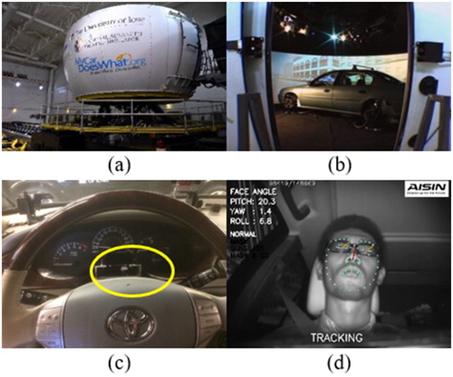
Aisin’s DMS, a production-ready device located on the steering column, was used to record driver state data through output data on the vehicle’s Controller Area Network (CAN) bus. The data were integrated into the simulator data stream and saved as part of NADS data files, as well as logged to local files. Aisin’s DMS is an infrared camera system that continuously monitors the driver for various states, including attentiveness, drowsiness, and distraction. The system detects the driver’s face and provides information such as head position and direction, eye gaze direction, distance between eyelids, blinking, etc. (see Figure 1). The effort described here uses only raw DMS signals and no proprietary state classification signals.

Experimental design

We collected data from 20 licensed adult drivers (50% female, age range 18–66). The experiment consisted of a 4-h drive along a 45-mile interstate nighttime loop, with a 15-min break halfway through. Participants drove between 10 p.m. and 2 a.m. They were required to be awake by 7 a.m. the day of the study visit, refrain from napping, and consume no caffeine after 1 p.m. We tracked activity with a Fitbit and they filled out a food and activity log. The drowsiness protocol was intentionally minimal compared to other drowsiness studies so the focus could be put on early stages of drowsiness, before obvious features such as long eye closures became detectable.

Drivers were instructed to drive as safely as possible. They were instructed to follow infrequent auditory route cues throughout the drive. They were not allowed to engage in other secondary tasks that could have interfered with drowsiness, such as using their phones or the radio. Beyond this, drivers were given no specific instructions about how to manage drowsiness or behave throughout the drive. They were allowed to set the cruise control using steering wheel controls.

A vigilance task was used throughout the drives. It was adapted from the Psychomotor Vigilance Task, a standard reaction time assessment to evaluate drowsiness (Dorrian et al. 2005). Although the vigilance task had the same interstimulus timing as the Psychomotor Vigilance Task, it was administered continuously throughout the drive. It is worth noting that the inclusion of the vigilance task may have delayed or offset some of the potential effects of drowsiness.

The drive contained light ambient traffic, a combination of heavy trucks, passenger vehicles, and other light trucks. On average, participants encountered 2 to 3 slower-moving vehicles and 2 to 3 faster-moving vehicles every 10 min. The spacing and order of this traffic within these 10-min segments was semirandom.

Dependent measures

Several dependent measures were computed as candidates for drowsiness detection features. Observer ratings of drowsiness (ORDs) was coded in real time during the drives (Wierwille and Ellsworth 1994). ORD provides an assessment of drowsiness on a 5-point scale, from awake to severely drowsy, based on a number of visual symptoms. In this study, ORD ratings were performed by a single rater, a trained observer watching a video feed of the driver’s face in real time during the drive. We also administered a vigilance task that measured reaction times via a finger-mounted button and recorded electrical brain activity via a 10-electrode EEG headset. Participants completed pre- and postdrive subjective ratings of drowsiness on the Stanford Sleepiness Scale (Hoddes et al. 1973). After evaluating and comparing the various measures of drowsiness collected in the study, ORD was selected as the ground truth for training and testing of the model.

A number of measures were computed from the data and lumped into either a vehicle-based sensor group or a driver-based sensor group. The vehicle-based measures were standard deviation of lane position, standard deviation of steering wheel angle, mean and standard deviation of steering reversal rate, and mean and standard deviation of small steering reversal rate. An extensive set of measures was computed from the DMS data relating to eye closure (including blinks and longer closures), eye gaze location, face orientation, and estimated distance between the nose and mouth. Around 45 separate measures were derived from this data and used to train drowsiness models. A complete summary of vehicle and driver-based measures is given in Table A1 (see online supplement).

Table 1. Model performance statistics with test set.

Statistic	VEH	DMS	BOTH	BIN
Accuracy	0.63	0.78	0.82	0.83
NIR	0.58	0.58	0.58	0.60
P value	<.001	<.001	<.001	<.001
Log loss	0.77	0.64	0.59	0.46
MROC	0.73	0.79	0.79	0.90^a

^a Traditional AUC.

Sampling

The ground truth ORD ratings were in the range 0–4, where 0 is not drowsy and 4 is extremely drowsy. ORD ratings occurred approximately every 10 min during each drive. Windows of data of 180 s were sampled from the simulator data, and they were allowed to overlap by 67%, or 2 min. All such windows that contained an ORD rating were included in the training and testing sets for the model. The raw simulator data were collected at 240 Hz but downsampled to 60 Hz for all postprocessing and analysis. The DMS unit used in the study had a sampling rate of 10 Hz, though more recent versions have gotten faster.

Modeling

The analysis and algorithm development was conducted using the R statistical programming language (R Core Team 2017). The caret library was used to develop machine learning models (Kuhn 2008). Of the many issues related to modeling, the first is determining what kind of model to make. We selected the random forest (Breiman 2001) due to its robustness against overgeneralization. The random forest is an ensemble model made up of a collection of decision trees. A simple majority of tree classifications is sufficient to set the classification from the forest.

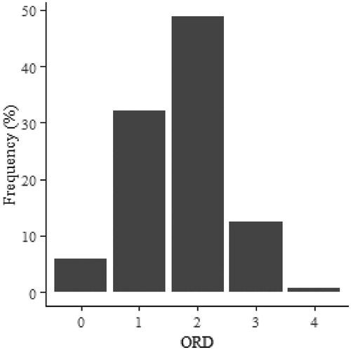
Due to imbalanced prevalence of observed ORD values (see Figure 2), the 5 values were collapsed to just 3 groups (ORD 0–1, ORD 2, ORD 3–4). Additionally, a binary model was developed that used the 2 drowsiness groups (ORD 0–1, ORD 2–4). To mitigate against problems associated with unbalanced samples, the Synthetic Minority Over-sampling Technique (SMOTE) method of resampling was used while training the model (Chawla et al. 2002). This procedure oversamples less prevalent values and undersamples more prevalent ones.

Figure 2. Distribution of ORD ratings among possible values (0–4).

The data used to train the model were normalized to reduce the effect of individual differences. After normalization, the training process should see ranges of values from each participant that are similar to one another. Consequently, any new data that are fed to the model for testing or prediction must also be normalized. Each driver’s data were normalized using their own mean and standard deviation for each variable. The normalization procedure involved the computation of the z-score for each variable under each driver, using the formula given in Eq. (1)(1) $$z=\mathrm{ }\frac{x-\mu }{\sigma }.$$(1) , where x is the raw input signal, µ is the mean of the signal, and σ is the standard deviation of the signal: (1) $$z=\mathrm{ }\frac{x-\mu }{\sigma }.$$(1)

Several procedures are available to mitigate against under- and overgeneralization while fitting a model. Two common ones are splitting the data into separate training and testing data sets and K-fold cross-validation, where the data are split into several folds, with each fold being iteratively held out in the training process. In this article, we take the view that these 2 approaches can be productively combined into a hybrid training strategy. We reserved all data from 2 participants as the testing set and then used 5-fold cross-validation on the remaining training set.

Research questions

Questions of interest in this research related to the efficacy of a commercial DMS to classify drowsiness when compared to vehicle-based sensors. Specifically the research was interested in the following questions:

1. What was the performance of models based on vehicle-based data, DMS data, and a combination of the two?

2. What levels of ORD could be effectively differentiated by the model?

3. What variables were most important for the classification of drowsiness?

A variable importance analysis that addresses the third question is relegated to the Appendix (see online supplement).

Results

Several measures of model performance are derived from the confusion matrix that counts instances of correct and incorrect classifications. Accuracy is one such measure and is reported directly by the caret model. It is computed as (2) $$\mathrm{Accuracy}=\mathrm{ }\frac{\mathit{TP}+\mathit{TN}}{\mathit{TP}+\mathit{TN}+\mathit{FP}+\mathit{FN}},$$(2) where TP and TN denote true positives and true negatives (appearing on the diagonal of the confusion matrix), and FP and FN denote false positives and false negatives (in the off-diagonals of the confusion matrix). The no information rate (NIR) is simply the prevalence of the most common class. The accuracy must be significantly higher than the NIR to be a compelling indicator of good performance, and this significance is reported as a P value in the testing set results.

Receiver operating characteristic (ROC) curves can be constructed for binary models, and the area under this curve (AUC) is another performance statistic. A multiclass ROC (MROC) measure is available for multiclass models and generalizes the AUC measure by averaging pairwise comparisons between classes (Hand and Till 2001). An alternative measure that does not come from the confusion matrix is log loss. It is useful in that it takes into account how much model predictions vary from the truth. A perfect model has 0 log loss.

The question of how to compare the various models arises. Comparisons are very simple in R for cross-validated models through the resamples function. Hypothesis tests for the equivalence of models are done from resamples using the techniques of Eugster et al. (2008) and Hothorn et al. (2005). However, the reported performance of the cross-validated model can look deceptively good; thus, we also reserved a testing set made up of data from 2 separate drivers. The performance of multiclass models on the testing data set was compared using McNemar’s test statistic. This statistic is computed as a chi-squared test on a contingency table that compares incorrect predictions of each model. It essentially tests whether the models are wrong in similar ways when trained on a common data set (Dietterich 1998).

Four participants had only partial DMS data recorded and were dropped from the modeling effort. Two participants’ data were reserved for the testing data set, leaving 14 participants’ data in the training set. Approximately 4 h of data were available per participant with ORD coded about every 10 min.

We trained a set of 3-class models using only vehicle signals (VEH), only DMS signals (DMS), and a combination of the two (BOTH). The best performance was observed with a combination of inputs; however, DMS signals were more important overall than vehicle signals. The minimum, average, and maximum accuracy observed during training under 5-fold cross-validation were 0.937, 0.946, 0.951 for the VEH model, 0.978, 0.987, 0.993 for the DMS model, and 0.986, 0.987, 0.988 for the BOTH model. Then, a binary model (BIN) was trained that was based on the BOTH model but with ORD levels 2–4 combined into a single class. The accuracy of this model was 0.996, 0.996, 0.997. A comparison of the 4 models using caret resamples revealed that DMS was significantly better than VEH (P = .003) but that BOTH was not significantly different than DMS (P = 1.000). However, BIN was significantly better than BOTH (P = .002).

Model performance was also measured on the testing set, consisting of data reserved from 2 drivers. Performance statistics are summarized in Table 1 for 4 models, and the confusion matrix for the BOTH model is shown in Table 2. The MROC version of AUC is reported for all models except BIN, which shows a traditional AUC. The ROC curve for BIN is shown in Figure 3. The blue shaded region shows the 95% confidence interval along the entire curve.

Figure 3. ROC curve for binary model.

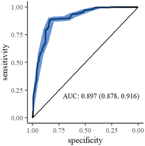
Table 2. Three-class model confusion matrix for prediction of ORDs.

Prediction	Reference
ORD	0–1	2	3–4
0–1	394	133	0
2	62	527	13
3–4	0	0	0

McNemar’s test indicated a significant difference between the DMS and VEH models, ${\chi }^2$(1) = 70.43, P < .001. There was also a significant difference between the BOTH model and the DMS model, ${\chi }^2$(1) = 30.42, P < .001. Given the structural change from 3-level to binary, McNemar’s test would not be appropriate to compare the BOTH and BIN models.

Discussion

Drowsy driving was studied in a driving simulator environment over the course of approximately 4 h per participant. Drowsiness was verified by periodic ORDs that were used as ground truth for a classification model. Random forest models were trained using vehicle signals, DMS signals, and a combination of the two. Overall, the DMS provided superior information to classify drowsiness, though the combination of both types of data should be used if available.

Increasing levels of automation are being integrated into vehicles that can take over both the speed-keeping and lane-keeping tasks from the driver. Crucially, we note that vehicle-based signals become unavailable when automation is engaged and will make the task of diagnosing driver impairment more challenging without camera-based driver monitoring.

The models were successful at discriminating lower levels of ORD (0–1) from moderate and severe levels (2–4); however, they were not effective at differentiating moderate drowsiness (ORD 2) from severe drowsiness (ORD 3–4). This is somewhat surprising because the expectation would be that more severe drowsiness would present more obvious symptoms that could be picked up by a DMS. The lower prevalence of severe drowsiness may have limited the ability of the model to accurately discern it. Severe drowsiness ratings were also not uniformly distributed among participants but were clustered heavily in a few, which limited options on how to split the testing and training sets.

Schleicher and colleagues (2008) discussed the fact that most microsleeps occur in stages of severe drowsiness; thus, an algorithm that relies on detecting them may act too late. The same argument applies to lane departures. It is thus quite encouraging that the algorithm presented here is able to discriminate lower levels of drowsiness from moderate and severe levels by relying on a variety of measures.

This research was limited by a relatively small sample size, though the amount of data produced was large. It is important to capture a wide range of individual behaviors, and more data would be helpful. All participants drove at the same time of day after a similar amount of time awake, thus removing time of day as a useful variable for training. The accuracy of some dependent measures was questionable given the low sampling rate of the device. They were left in the model because hardware is always improving and because any signals dominated by noise should not have much influence on the classification performance. ORD is a subjective measure of drowsiness that is satisfying from the perspective of “I know it when I see it.” It was limited to some degree by the sparsity of ORD ratings and the use of only a single rater. Further improvements in drowsiness detection systems may be expected due to several factors, including improved hardware, the addition of unobtrusive physiological measures from heart rate sensors and wearables, and the intelligent integration of environmental variables such as time of day and time on task.

Acknowledgments

The authors gratefully acknowledge the contributions of Harry Torimoto, Alan Arai, Hiroyuki Yogo, and the dedicated staff of NADS in organizing and carrying out this research. Aisin provided the DMS hardware and NADS staff integrated it into the simulation environment. John Gaspar designed the scenarios and ran the study, and Chris Schwarz analyzed the data and created the models.

Additional information

Funding

This research was funded by the Aisin Technical Center of America.

References

- Balkin TJ, Horrey WJ, Graeber RC, Czeisler CA, Dinges DF. The challenges and opportunities of technological approaches to fatigue management. Accid Anal Prev. 2011;43:565–572.
- Breiman L. Random forests. Mach Learn. 2001;45:5–32.
- Chawla NV, Bowyer KW, Hall LO, Kegelmeyer WP. SMOTE: synthetic minority over-sampling technique. J Artif Intell Res. 2002;16:321–357.
- Dietterich TG. Approximate statistical tests for comparing supervised classification learning algorithms. Neural Comput. 1998;10:1895–1923.
- Dinges DF, Grace R. PERCLOS: A Valid Psychophysiological Measure of Alertness as Assessed by Psychomotor Vigilance. Washington, DC: U.S. Department of Transportation, Federal Highway Administration; 1998. Publication Number FHWA-MCRT-98-006.
- Dorrian J, Rogers NL, Dinges DF. Psychomotor Vigilance Performance: Neurocognitive Assay Sensitive to Sleep Loss. New York, NY: Marcel Dekker; 2005.
- Eugster MJ, Hothorn T, Leisch F. Exploratory and Inferential Analysis of Benchmark Experiments Department of Statistics: Technical Reports, No. 30, 2008.
- Federal Highway Administration. Roadway departure safety. 2018. Available at: https://safety.fhwa.dot.gov/roadway_dept/. Accessed April 26, 2018.
- Fitzharris M, Liu S, Stephens AN, Lenné MG. The relative importance of real-time in-cab and external feedback in managing fatigue in real-world commercial transport operations. Traffic Inj Prev. 2017;18(Suppl. 1):S71–S78.
- Hand DJ, Till RJ. A simple generalisation of the area under the ROC curve for multiple class classification problems. Mach Learn. 2001;45(2):171–186.
- Hoddes E, Zarcone V, Smythe H, Phillips R, Dement WC. Quantification of sleepiness: a new approach. Psychophysiology. 1973;10:431–436.
- Hothorn T, Leisch F, Zeileis A, Hornik K. The design and analysis of benchmark experiments. J Comput Graph Stat. 2005;14:675–699.
- Krajewski J, Sommer D, Trutschel U, Edwards D, Golz M. Steering wheel behavior based estimation of fatigue. Paper presented at: Fifth International Driving Symposium on Human Factors in Driver Assessment, Training and Vehicle Design; 2009; Big Sky, MT.
- Kuhn M. Building predictive models in R using the caret package. J Stat Softw. 2008;28(5):1–26.
- Kuo J, Lenné MG, Mulhall M, et al. Continuous monitoring of visual distraction and drowsiness in shift-workers during naturalistic driving. Saf Sci. 2018.
- McDonald AD, Lee JD, Schwarz C, Brown TL. Steering in a random forest: ensemble learning for detecting drowsiness-related lane departures. Hum Factors. 2014;56:986–998.
- McDonald AD, Schwarz C, Lee JD, Brown TL. Real-time detection of drowsiness related lane departures using steering wheel angle. Proc Hum Factors Ergon Soc Annu Meet. 2016;56:2201–2205.
- NHTSA. 2016 Fatal Motor Vehicle Crashes: Overview. Washington, DC: Author; 2016. DOT HS 812 456.
- Owens J, Dingus T, Guo F, et al. Prevalence of Drowsy-Driving Crashes: Estimates from a Large-Scale Naturalistic Driving Study. Washington, DC: AAA Foundation for Traffic Safety; 2018.
- R Core Team. R: A Language and Environment for Statistical Computing [computer program]. Vienna, Austria: R Foundation for Statistical Computing; 2017.
- Schleicher R, Galley N, Briest S, Galley L. Blinks and saccades as indicators of fatigue in sleepiness warnings: looking tired? Ergonomics. 2008;51:982–1010.
- Sinha O, Singh S, Mitra A, Ghosh S, Raha S. Development of a drowsy driver detection system based on EEG and IR-based eye blink detection analysis. In: Advances in Communication, Devices and Networking. Singapore: Springer; 2018:313–319.
- Tateno S, Guan X, Cao R, Qu Z. Development of drowsiness detection system based on respiration changes using heart rate monitoring. Paper presented at: 2018 57th Annual Conference of the Society of Instrument and Control Engineers of Japan (SICE); 2018.
- Wei C-S, Wang Y-T, Lin C-T, Jung T-P. Toward drowsiness detection using non-hair-bearing EEG-based brain–computer interfaces. IEEE Trans Neural Syst Rehabil Eng. 2018;26:400–406.
- Wierwille WW, Ellsworth LA. Evaluation of driver drowsiness by trained raters. Accid Anal Prev. 1994;26:571–581.
- Yamakawa T, Fujiwara K, Hiraoka T, et al. Validation of HRV-based drowsy-driving detection method with EEG sleep stage classification. Sleep Med. 2017;40:e352.