Multi-sensor driver monitoring for drowsiness prediction

Abstract

Objective

Driver monitoring systems are growing in importance as well as capability. This paper reports drowsy driving detection models that use vehicular, behavioral, and physiological data. The objectives were to augment camera-based system with vehicle-based and heart rate variability measures from a wearable device and compare the performance of drowsiness detection models that use these data sources. Timeliness of the models in predicting drowsiness is analyzed. Timeliness refers to how quickly a model can identify drowsiness and, by extension, how far in advance of an adverse event a classification can be given.

Methods

Behavioral data were provided by a production-type Driver Monitoring System manufactured by Aisin Technical Center of America. Vehicular data were recorded from the National Advanced Driving Simulator’s large-excursion motion-base driving simulator. Physiological data were collected from an Empatica E4 wristband. Forty participants drove the simulator for up to three hours after being awake for at least 16 hours. Periodic measurements of drowsiness were recorded every ten minutes using both observational rating of drowsiness by an external rater and the self-reported Karolinska Sleepiness Scale. Nine binary random forest models were created, using different combinations of data sources and ground truths.

Results

The classification accuracy of the nine models ranged from 0.77 to 0.92 on a scale from 0 to 1, with 1 indicating a perfect model. The best-performing model included physiological data and used a reduced dataset that eliminated missing data segments after heartrate variability measures were computed. The most timely model was able to detect the presence of drowsiness 6.7 minutes before a drowsy lane departure.

Conclusions

The addition of physiological measures added a small amount of accuracy to the model performance. Models trained on observational ratings of drowsiness detected drowsiness earlier than those based only on Karolinska Sleepiness Scale, making them more timely in detecting the onset of drowsiness.

Keywords:

• Drowsy driving
• driver monitoring system
• vehicle safety

Introduction

Driver monitoring systems (DMS) are growing in importance as well as capability. The integration of DMS into a vehicle cabin may allow systems and automation to respond better to driver behaviors and build a cooperative, assistive relationship between driver and vehicle. DMS technology supports partially automated driving systems, driver impairment countermeasures, and occupancy detection, among a growing list of applications.

Drowsiness detection techniques can be loosely categorized into behavioral, vehicular, and physiological approaches (Ramzan et al. 2019). Behavior measures include eye/blink measures and facial expressions. Vehicular measures include steering and lane-keeping variables. Physiological measures capture signals from the brain, heart, respiration, and skin. Utilization of these measures in commercial systems was detailed in a recent review (Doudou et al. 2020).

Machine learning models are adept at integrating many different variables and finding their underlying connection to a variable or state of interest. Drowsiness models commonly rely on support vector machines, hidden Markov models, and deep learning with convolutional neural networks (Ramzan et al. 2019). The authors have also used random forests to good effect in detecting drowsy driving (McDonald et al. 2014; Schwarz et al. 2019).

This study used behavioral data from a commercial DMS, vehicular data recorded from the National Advanced Driving Simulator’s large-excursion motion-base driving simulator, and physiological data from a wristband. The current project builds on a prior study with an earlier generation DMS (Schwarz et al. 2019) by using more capable hardware, adding additional ground truth, including physiological data measures, and including a deeper investigation of timeliness. The objectives of the study were to evaluate the added benefit of including physiological data from a wearable on the performance of drowsiness detection models, and to collect quantitative measures of model timeliness.

Methods

Apparatus

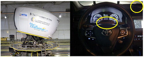
Data were collected using the high-fidelity full-motion NADS-1 simulator at the National Advanced Driving Simulator at the University of Iowa. The simulator consists of a 24-foot diameter dome enclosing a full-size 2014 Toyota Camry sedan with active steering and pedal feedback. A 13-degree of freedom motion system provides participants accurate acceleration, braking, and steering cues they expect from driving (see Figure 1, left). Sixteen high-definition (1920 × 1200) LED (light emitting diode) projectors display seamless imagery on the interior walls of the dome with a 360-degree horizontal field of view. The data sampling rate was 240 Hz. Aisin Technical Center of America (from Aisin Group) supplied two separate production-type Driver Monitoring System (DMS) units which were integrated into the Camry cab (see Figure 1, right). One was installed on the steering column, while the other was mounted on the dash above the center console. In this work only data from the steering column unit was used. Physiological data were collected using an Empatica E4 wristband, a photoplethysmography sensor that optically measures blood volume pulse (BVP). In addition to collecting physiological data during the drive from the E4, breathing and heartrate were also collected with a non-contact, millimeter-wave radar.

Figure 1. NADS-1 large excursion motion base (left), cabin interior with two DMS units (right).

Experiment design

Data were collected from 40 licensed drivers (20 male and 20 female) with a range of age (mean 37.7 ± 9.62 years). All study procedures were approved by the University of Iowa Institutional Review Board (IRB #202004192). Participants drove a 3-hour simulated route, with an interstate loop and light ambient traffic, following the initial DMS study (Schwarz et al. 2019). The experiment was designed such that each participant began the drive after at least 16 hours of continued wakefulness, which previous NHTSA drowsiness research at the NADS has shown to increase severe drowsiness and drowsy lane departures (Gaspar et al. 2017).

Participants arrived at 10 pm and began the study drive at 11 pm or 2:30am (there were two slots each night). Prior to the study drive, the Empatica E4 wristband collected baseline physiological signals while the participant remained seated for ten minutes. Participants then sat in a conference room and were asked to remain awake until their drive began. They could watch movies, work, play games, or read, but were not allowed to consume caffeine or exercise.

Every ten minutes during the drive, a remote researcher monitored the driver for one minute and entered an observational rating of drowsiness (ORD). After each ORD, participants answered a Karolinska Sleepiness Scale (KSS) question on a tablet. Subjective ratings are often done before and/or after a drive. Wang and Xu (2016) also administered it halfway through their drive, at the 30 minute mark. A 10 minute probe interval offers a higher resolution view of drowsiness while interfering minimally with the impaired state itself.

Dependent measures

Data from the various sources were used to compute a set of dependent measures. Some of these measures were selected as features for training the drowsiness models. Three types of dependent measures were considered: vehicle, driver, and physiological. The ORD and KSS measures collected at ten-minute intervals served as direct measures of drowsiness and were used as ground truth to test model performance. Vehicular measures came from simulator variables that included mean time-to-lane crossing, standard deviation of lane position, mean lane departure duration, steering reversal rate, and high frequency steering (Merat et al. 2014).

The largest set of dependent measures were behavioral, extracted from the real-time DMS data. These included head position and orientation, vertical and horizontal gaze angle, blink frequency and duration, eye opening/closing/reopening duration, closed-to-blink ratio, blink waveform area, percent road center (PRC), and percent eyelid closure (PERCLOS). Of these measures, some were computed as means and standard deviations over a window while others (PRC, PERCLOS) are already defined as scalar values.

Physiological data were collected from the Empatica E4 wristband and used to estimate heartrate variability (HRV) measures: mean, standard deviation, and root-mean-square of normal-normal (NN) intervals, HRV triangle index (HRVTI), low-frequency spectrum (LF), high-frequency spectrum (HF), normalized LF and HF, and LF-HF ratio.

Data processing

Data were converted and collated in Matlab and physiological data were synchronized with the simulator data using initial timestamps. The Empatica E4 uses a proprietary algorithm to estimate inter-beat intervals (IBI), equivalent to NN intervals. From a smoothed inverse of the IBI it reports heartbeat. The IBI estimation algorithm is conservative, meaning that a manual review of both BVP and IBI reveals many additional intervals that could be marked. We developed an algorithm to identify additional intervals while still rejecting noisy data segments. It proceeds by computing some statistical properties of known IBIs that were identified by Empatica and searching for other intervals that match those properties. It concludes by eliminating IBIs that are larger or smaller than expected (Malik et al. 1989). Whereas Malik allowed a 20% variability between IBI samples, we increased that to a generous 30% threshold. Spectrum-based HRV measures were computed using the Lomb-Scargle periodogram which has the benefit of working directly on irregularly spaced IBI samples (Estévez et al. 2016; Stewart et al. 2020).

While some DMS measures are straightforward to compute, blinks are tricky to capture and results may be sensitive to implementation details. We followed the systematic algorithm of Baccour et al. (2019). All DMS variables were first interpolated to match the sampling rate (60 Hz) of the simulator data. The algorithm proceeds by estimating peak eye closing and opening velocities as well as the blink start and end. From those basic parameters, several blink measures can be derived. As in the paper, the threshold for detecting peak closing velocity is adjusted every five minutes with a k-means clustering to separate blinks from non-blinks.

HRV measures were computed over five-minute windows and all other measures were computed over three-minute windows. Measures were updated every minute. In the case of missing data, of which there was a considerable amount for HRV measures, not-a-number (NaN) values were recorded. Some measures, now sampled at 0.1 Hz, were one-sided and had long-tailed distributions; therefore, log transformations were applied to normalize their distributions. This was not done to satisfy any normality requirements imposed by the modeling technique as there were no assumptions. Rather, it helped in the Z-score normalization process that assumes variability can be characterized using only means and standard deviations. Z-scores for each measure were computed using data segments with ORD less than two. These statistics were applied to measures over all time to obtain the normalized and scaled measure in Eq. (1)(1) $$Z\mathrm{ }=\mathrm{ }\frac{x-\mu }{\sigma }$$(1) . (1) $$Z\mathrm{ }=\mathrm{ }\frac{x-\mu }{\sigma }$$(1) where x denotes the original measure (possibly log-transformed) and μ and σ denote the mean and standard deviation over all non-drowsy samples. The Z-score process is an effective method to normalize away differences observed among individual drivers (Walker et al. 2019).

Results

Data analysis was conducted with the R statistical language (R Core Team 2017) using the ascii data files generated in the data reduction step. Random forest models were created with the Caret package (Kuhn 2008), using the “RF” model specification. We first present models with only driver and vehicle data that make use of all participants. Then, we reduce the dataset to include those participants with sufficient quality HRV data and add the physiological group to the model. Reduced-dataset models without HRV were also trained.

Data from eight participants were reserved from the full dataset of 40 participants. The reduced dataset is comprised of data from only 16 participants. While almost all participants had some non-noisy HRV data, we conservatively eliminated all participants for which the amount of good HRV data was less than around 25% of the total. Data from three participants were reserved from the reduced dataset for testing. In both cases the test dataset was selected to maintain a representative balance of ground truth levels.

We trained models with three choices for ground truth, one where drowsiness was defined as KSS ≥ 8, one where it was defined as ORD ≥ 2, and a combined metric in which either of the first two thresholds indicated drowsiness. We adopt a naming convention for the models that uses F or R for full or reduced and K, O, or C for KSS, ORD, or combined, respectively. The letter H is appended to the label if HRV data was included. In all the reported models, the positive class in the confusion matrix corresponds to not drowsy.

Table 1 shows performance statistics for the models created from the full dataset. Accuracy is reported within the range of its 95% confidence interval. The no-information rate (NIR) is related to the prevalence of each class and is important to consider. For example, if the non-drowsy class is 90% prevalent, then NIR would be 0.9 and an algorithm could achieve 90% accuracy by always guessing not drowsy. Sensitivity and specificity provide measures of the true and false positive rates, but are independent of prevalence. Positive and negative predictive value incorporate prevalence into their calculation. Results from the reduced dataset are given in Tables 2 and 3, in which the former still uses only behavior and vehicular measures while the latter also includes physiological measures. Two types of timeliness were computed, based on the occurrence of drowsy lane departures (DLD). A DLD is defined as a lane departure lasting at least one second associated with an ORD value of at least two. Lane departures with lower ORD values were also captured and classified as normal or ‘alert’ departures. The first timeliness measure is defined as the time between the first drowsiness classification and the first DLD, in minutes, and is included in Tables 1–3. The most timely model (FC) was able to classify drowsiness 6.7 minutes prior to the first DLD. The second timeliness measure considers all lane departures, both normal and drowsy, throughout the drives, and checks whether there is a drowsiness classification in the three minutes before and including the departure. Ideally we hope to see such a classification prior to DLDs but not prior to normal lane departures. Since the resolution of the data is minute by minute, we assume the actual lead time considered by this method to be uniformly distributed between two and three minutes, on average 2.5 minutes.

Table 1. Models created with full dataset.

	FK	FO	FC
Accuracy	(.74, .77, .79)	(.78, .81, .83)	(.76, .78, .80)
NIR	.51	.58	.62
Sensitivity	.82	.70	.63
Specificity	.72	.88	.88
PPV	.74	.81	.76
NPV	.81	.81	.79
Timeliness	−14.7	3	6.7

Table 2. Models created with reduced dataset.

	RK	RO	RC
Accuracy	(.77, .82, .86)	(.86, .90, .93)	(.85, .89, .92)
NIR	.52	.61	.61
Sensitivity	.77	.89	.81
Specificity	.87	.91	.94
PPV	.87	.86	.90
NPV	.78	.93	.89
Timeliness	−13.3	1	1.3

Table 3. Models created with reduced dataset and physiological measures.

	RKH	ROH	RCH
Accuracy	(.81, .85, .89)	(.87, .91, .94)	(.88, .92, .95)
NIR	.52	.61	.61
Sensitivity	.77	.95	.89
Specificity	.94	.88	.93
PPV	.93	.84	.89
NPV	.79	.96	.93
Timeliness	−13.3	1	1.3

An ORD of 2 indicates slight drowsiness but a KSS of 8 means sleep with some effort to keep awake. A model trained on a KSS of 7 might be more timely. We considered this as a candidate model and compared it to the one trained on KSS > =8. With a lower KSS threshold, the model had lower sensitivity (.61), higher specificity (.84), and better first-time timeliness (-7.57). Lower sensitivity means that more non-drowsy samples were incorrectly classified as drowsy (false positives). This could inadvertently improve the timeliness; however, the KSS models were still not nearly as timely as ORD or combined models (negative timeliness means detection after the first DLD).

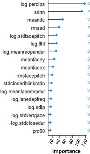
The relative importance of each measure is readily available from the model information. This importance is plotted in Figure 2 for the best performing model, RCH. Each measure is annotated according to the group it belongs to. Of 17 measures used in the model, 10 were behavioral, 4 were vehicular, and 3 were physiological. The log of PERCLOS and SDNN appear to be the two most important variables for the performance of the RCH model by a fair amount.

Figure 2. Variable importance plot for model RCH. Annotated with group: (B)ehavioral, (V)ehicular, or (P)hysiological.

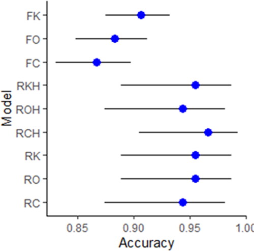
From the second timeliness calculation, a complete set of statistics can be computed from its confusion matrix, in which the positive class corresponds to a normal lane departure and the negative class to a DLD. Figure 3 shows the accuracy, within the 95% confidence interval, of the timeliness metric for all models.

Figure 3. Timeliness accuracy throughout drives, with 95% confidence intervals.

Discussion

There was a large amount of missing physiological data. Only 16 of 40 participant datasets were analyzed and there was a considerable amount of missing data even in the kept data (though we were conservative by completely eliminating participants that had too little good HRV data). The delicate nature of trying to collect physiological data through contact sensors makes data quality a difficult issue. In the laboratory environment we may have been able to limit noisy data by tightening the E4 wristband more, checking baseline data before proceeding to the main drive, or using a different sensor to record heart rate. However, the prospect of collecting physiological data in this manner from drivers in a naturalistic setting seems fraught. It might also help to wear the sensor on a body part that doesn’t move as much while driving as the hands do, or to use a sensor with a higher sampling frequency (the E4 collects BVP at 64 Hz).

There is a marked difference in performance observed between the full and reduced datasets with the latter exhibiting much larger accuracy values. The test portion of the reduced dataset was only three participants, but that represented about 23% of the data. We wondered whether an extreme type of overfitting known as double descent was in effect due to the smaller dataset, but that phenomenon is normally observed in much larger deep learning models. More likely the results stemmed from the specific subset of participants that were kept. Due to the smaller sample size, we would expect the results could vary greatly when configured differently, say when reserving a different set of participants on which to test.

There was a small bump in performance with the physiological measures, but less than one might expect. While HRV measures have been observed to be sensitive to drowsiness, our results point to the importance of good quality data and the difficulty inherent in collecting clean data from wearables. This is especially true with measures around HRV that rely on small second-to-second variations in heartbeat. Nevertheless, three of the top six important variables in the RCH model were HRV measures. It could be that measures from the different groups don’t stack in a linear way, but represent different dimensions that relate to subjective measures of drowsiness in different ways. A simplistic way this might occur is that each measure group might have its own optimal threshold to differentiate binary drowsiness.

Timeliness refers to how quickly a model can identify the condition of interest, or how far in advance of an adverse event a classification can be given. In this application, we desire to identify drowsiness and be able to act on that information before the driver falls asleep or suffers a significant lane departure event. Toward this end we computed first-time timeliness as well as the 2.5 minute timeliness accuracy throughout each drive. First-time timeliness is a more compelling measure for a couple of reasons. First, the chances of a crash increase the longer drowsiness exists and for each cumulative occurrence of a DLD, making warnings less effective later on. Second, we would expect subsequent DLDs to be impacted (hopefully eliminated) in the presence of a countermeasure. Either a driver will pay attention to drowsiness warnings and take a break, or they will tune them out.

The models presented here are most useful to catch the onset of drowsiness. A holistic drowsiness mitigation system should combine them with other inputs such as environment variables (time of day, time on task, traffic density) and imminent warnings (collision warning systems, sleep detection). The accuracy reported here is in line with published drowsiness work (Albadawi et al. 2022), though accuracy alone is insufficient to judge most models since it does not reveal class imbalance issues or tradeoffs between false positives and false negatives. Moreover, different choices for ground truth can greatly impact the results. Our measurement of KSS and ORD every 10 minutes was able to pinpoint changes in the drowsiness state better than studies that only measured it before and after, or every 30 minutes. It is true that models trained on simulator data may not generalize to all driving conditions in the real world, and this limitation should be addressed by adding on-road and naturalistic data to the model. Future work will attempt to use the millimeter-wave radar data to compute respiration and heartbeat measures. Additionally, we plan to combine drowsiness data from multiple simulator studies conducted over a number of years to strengthen the models.

Additional information

Funding

This project was funded by Aisin Technical Center of America (from Aisin Group).

References

- Albadawi Y, Takruri M, Awad M. 2022. A review of recent developments in driver drowsiness detection systems. Sensors. 22(5):2069. doi: 10.3390/s22052069
- Baccour MH, Driewer F, Kasneci E, Rosenstiel W. 2019. Camera-based eye blink detection algorithm for assessing driver drowsiness. Paper presented at: 2019 IEEE Intelligent Vehicles Symposium (IV). p. 987–993. doi: 10.1109/IVS.2019.8813871.
- Doudou M, Bouabdallah A, Berge-Cherfaoui V. 2020. Driver drowsiness measurement technologies: current research, market solutions, and challenges. Int J ITS Res. 18(2):297–319. doi: 10.1007/s13177-019-00199-w.
- Estévez M, Machado C, Leisman G, et al. 2016. Spectral analysis of heart rate variability. Int J Disabil Hum Dev. 15(1):5–17. doi: 10.1515/ijdhd-2014-0025.
- Gaspar JG, Brown TL, Schwarz CW, Lee JD, Kang J, Higgins JS. 2017. Evaluating driver drowsiness countermeasures. Traffic Inj Prev. 18(sup1):S58–S63. doi: 10.1080/15389588.2017.1303140.
- Kuhn M. 2008. Building predictive models in R using the caret package. J Stat Softw. 28(5):1–26. doi: 10.18637/jss.v028.i05.
- Malik M, Cripps T, Farrell T, Camm A. 1989. Prognostic value of heart rate variability after myocardial infarction. A comparison of different data-processing methods. Med Biol Eng Comput. 27(6):603–611. doi: 10.1007/BF02441642.
- McDonald AD, Lee JD, Schwarz C, Brown TL. 2014. Steering in a random forest: ensemble learning for detecting drowsiness-related lane departures. Hum Factors. 56(5):986–998. doi: 10.1177/0018720813515272.
- Merat N, Jamson AH, Lai FCH, Daly M, Carsten OMJ. 2014. Transition to manual: driver behaviour when resuming control from a highly automated vehicle. Transp Res Part F: Traffic Psychol Behav. 27:274–282. doi: 10.1016/j.trf.2014.09.005.
- Ramzan M, Khan HU, Awan SM, Ismail A, Ilyas M, Mahmood A. 2019. A survey on state-of-the-art drowsiness detection techniques. IEEE Access. 7:61904–61919. doi: 10.1109/ACCESS.2019.2914373.
- R Core Team. 2017. A language and environment for statistical computing. Vienna, Austria. https://www.R-project.org/.
- Schwarz C, Gaspar J, Miller T, Yousefian R. 2019. The detection of drowsiness using a driver monitoring system. Traffic Inj Prev. 20(sup1):S157–S161. doi: 10.1080/15389588.2019.1622005.
- Stewart J, Stewart P, Walker T, Gullapudi L, Eldehni MT, Selby NM, Taal MW. 2020. Application of the Lomb-Scargle Periodogram to investigate heart rate variability during haemodialysis. J Healthc Eng. 2020:8862074. doi: 10.1155/2020/8862074.
- Walker F, Wang J, Martens MH, Verwey WB. 2019. Gaze behaviour and electrodermal activity: objective measures of drivers’ trust in automated vehicles. Transp Res Part F: Traffic Psychol Behav. 64:401–412. doi: 10.1016/j.trf.2019.05.021.
- Wang X, Xu C. 2016. Driver drowsiness detection based on non-intrusive metrics considering individual specifics. Accid Anal Prev. 95(Pt B):350–357. doi: 10.1016/j.aap.2015.09.002