An ALNS-based approach for the traffic-police-routine-patrol-vehicle assignment problem in resource allocation analysis of traffic crashes

Abstract

Objectives

Imbalances between limited police resource allocations and the timely handling of road traffic crashes are prevalent. To optimize resource allocations and route choices for traffic police routine patrol vehicle (RPV) assignments, a dynamic crash handling response model was developed.

Methods

This approach was characterized by two objective functions: the minimum waiting time and the minimum number of RPVs. In particular, an adaptive large neighborhood search (ALNS) was designed to solve the model. Then, the proposed ALNS-based approach was examined using comprehensive traffic and crash data from Ningbo, China.

Results

Finally, a sensitivity analysis was conducted to evaluate the bi-objective of the proposed model and simultaneously demonstrate the efficiency of the obtained solutions. Two resolution methods, the global static resolution mode, and real-time dynamic resolution mode, were applied to explore the optimal solution.

Conclusions

The results show that the optimal allocation scheme for traffic police is 13 RPVs based on the global static resolution mode. Specifically, the average waiting time for traffic crash handling can be reduced to 5.5 min, with 53.8% less than 5.0 min and 90.0% less than 10.0 min.

Keywords:

• Traffic safety
• traffic crash
• routine patrol vehicles (RPVs;), adaptive large neighborhood search (ALNS;), traffic police

Introduction

The global road traffic safety situation remains severe and complex. According to the World Health Organization (WHO), road traffic deaths in 182 countries are still as high as 1.3 million per year (World Health Organization 2019). Road traffic accidents have been recognized as one of the major public hazards in all categories (McIlroy et al. 2019; Wang et al. 2019; Ding et al. 2022; Li and Zhao 2022; Ding et al. 2023).

Rapid scientific responses, timely dispatches and crash data collection are essential elements of urban road safety prevention and control and can be used to reduce the severity of road traffic crash damages and manage traffic accident occurrences (Wong and Manning 2022). However, the shortage of urban traffic police, especially the number of traffic police routine patrol vehicles (RPVs), significantly affects the responses to traffic crashes and the disposal of these crashes. For example, there were approximately 8,809,984 traffic violations in Ningbo in 2021. However, the number of traffic police officers, only 303 officers patrolling the region, must be increased. Additionally, the number of traffic-police-RPVs is much fewer than that required for urban road traffic development and management tasks (Peng et al. 2023).

Thus, it is paramount to optimize the allocation of limited police resources, including traffic police and traffic-police-RPVs. According to the “Regulations on Procedures for Handling Road Traffic Accidents” in China, traffic police should be dispatched within 5 min after receiving incident orders and within 10 min during the nighttime. This study proposes a dynamic crash-handling response model to optimize resource allocations and route choices for traffic police RPVs. This approach can be characterized by two objective functions: the minimized waiting time for crash handling and the minimized number of traffic-police-RPVs. Furthermore, an adaptive large neighborhood search (ALNS) will be applied to determine the optimal solution.

Literature review

Allocation planning of traffic-police-RPV resources

Allocation planning of traffic-police-RPV resources can be categorized into two aspects: macroplanning problems (Hoque et al. 2004; Krukowski and Siemiński. 2018; Koskey and Njoroge 2019; Ho 2020) and microplanning problems (Kolesar et al. 1975; Sacks 2000; Heyer et al. 2008; Sayarshad 2022). Specifically, macroplanning traffic-police-RPV resources aim to balance the work demand by integrating decision-making on the number of traffic-police-RPVs, path selection, resource scheduling, etc. Representative theories include new public management theory (Krukowski and Siemiński 2018), administrative efficiency theory (Nepomuceno et al. 2021), two-factor theory (Munyeka and Setati 2022), no-growth improvement theory (Luan et al. 2022), weighted management theory (Jagat 2021), and systems principles (Terpstra and Schaap 2021). In contrast, the microplanning traffic-police-RPV resources are oriented to the specific task demands. For instance, the optimal number of traffic-police-RPVs can be estimated by evaluating the task demand workload and efficiency. The representative theories of microplanning problems include queuing theory (Ahmad and Jayalalitha 2021), linear regression theory (Aiello 2021), and the DEA model (Wong and Manning 2022).

Dispatching of traffic-police-RPV resources

Traffic-police-RPV resource dispatching refers to the optimal matching of traffic-police-RPV resources and the optimal dispatching path. In previous studies, there were three common theories for the optimal matching of traffic-police-RPV resources, including exact matching theories (e.g., Hungarian assignment algorithm and dynamic programming theory), approximate matching theories (e.g., fuzzy mathematical theory and greedy algorithm), and pattern-specific matching theories (e.g., prediction-based algorithms, clustering algorithm, and lattice algorithm). Although the efficiency of these methods was widely illustrated, they were designed for route optimization in conventional patrol or scheduling, in which the tasks or scheduling demands were all known before optimization and failed to handle traffic emergency disposals. Because the tasks/demands or available resources of emergency scheduling were unknown before optimization, the scheduling was required to be fast. For instance, most are passively waiting for response methods and manual assignments based on location information services.

The optimal dispatching path aims to search the optimal path between the task point and the disposal traffic-police-RPVs, considering the current traffic state and organization of the road network (Kovacs et al. 2012). In the literature, two common path decision algorithms, the exact algorithm, and heuristic algorithm, were adopted (Tamannaei and Irandoost 2019; Archetti et al. 2020; Mahmutoğulları et al. 2023; Hu et al. 2021; Liu et al. 2017; Li and Zhao 2022; Adulyasak et al. 2014; Azi et al. 2014; Dayarian et al. 2016). Examples include exact algorithms (e.g., the branch-and-bound method and Bender’s decomposition algorithm) and heuristic algorithms (e.g., the ant colony algorithm, simulated annealing algorithm, forbidden search algorithm, genetic algorithm, and adaptive large neighborhood search algorithm). The exact algorithm that can achieve a high-quality solution cannot obtain an optimal solution in an acceptable time under a large-scale problem. In contrast, the heuristic algorithm can obtain a suboptimal solution in a shorter period by making a tradeoff between the solution’s quality and efficiency.

Methodology

Problem description

The problem can be described as an optimal assignment problem for N traffic-police-RPVs to handle M crash tasks in a day according to the working conditions of the traffic-police-RPVs, assuming N<<M. Details of the problem description are as follows.

1. One crash should be handled by one traffic police RPV and one police officer.

2. Crash rankings (i.e., codes) can be confirmed based on the occurrence time.

3. The maximum waiting time for a crash is determined by the crash severity level.

4. The crash handle time by the traffic police RPV is assumed to be a normal-distribution with the parameters (μ, σ²).

5. A dynamic mechanism between traffic police RPVs and crash matching is designed. In particular, 24 hours will be divided into K time panes based on the distribution of traffic incidents. The free traffic-police-RPVs will be assigned to undisposed traffic crashes in each time pane.

6. Since the number of undisposed crashes may be greater than the number of available traffic-police-RPVs in the time panes, we assume that crashes that are not successfully matched to traffic-police-RPVs in the current time pane will be deferred to the next time pane.

7. A traffic-police-RPV can only be assigned one traffic crash in each time pane.

8. The traffic-police-RPV does not need to return to the police command center when finishing the current assignment. They can continue to perform patrol duties on the road until they receive the next task.

Modeling

Objective function

According to the above problem description, formulations of the proposed model are given as follows: (1) $$\mathrm{\text{min}}\hspace{0.17em}Z=\sum _{k=1}^K\left[\sum _{m=1}^M\sum _{n=1}^N\left(t_{\mathit{\text{mn}}}{\left(k\right)x}_{\mathit{\text{mn}}}\right){\delta }_{\mathit{\text{mk}}}+\sum _{m=1}^M\left(p_k-p_m\right){\delta }_{\mathit{\text{mk}}}\right]$$(1) (2) $$\mathit{\text{mi}}nF=N$$(2)

In Equation (1)(1) $$\mathrm{\text{min}}\hspace{0.17em}Z=\sum _{k=1}^K\left[\sum _{m=1}^M\sum _{n=1}^N\left(t_{\mathit{\text{mn}}}{\left(k\right)x}_{\mathit{\text{mn}}}\right){\delta }_{\mathit{\text{mk}}}+\sum _{m=1}^M\left(p_k-p_m\right){\delta }_{\mathit{\text{mk}}}\right]$$(1) , the objective function Z refers to the minimum waiting time for the crash, which consists of two parts: the matching time and travel time of traffic-police-RPVs. In Equation (2)(2) $$\mathit{\text{mi}}nF=N$$(2) , N denotes the number of RPVs. This value can affect the feasible domain of the solution. If the value of N is too small, there will be no feasible solution; if the value of N is too large, the solution might not satisfy the objective of the minimum number of RPVs.

The symbols used in the objective function are shown as follows:

$t_{\mathit{\text{mn}}}(k)$: The travel time of RPV n to Crash m (unit: minute) in Time Pane $k$.

$x_{\mathit{\text{mn}}}$: If $x_{\mathit{\text{mn}}}=1$, RPV n is assigned to Crash m; otherwise, $x_{\mathit{\text{mn}}}=0$.

$t_{\mathit{\text{mn}}}(k)x_{\mathit{\text{mn}}}$: The shortest travel time of RPV n to Crash m in the k-th time pane.

${\delta }_{\mathit{\text{mk}}}$: If ${\delta }_{\mathit{\text{mk}}}=1$, Crash m occurs within Period $k$; otherwise, ${\delta }_{\mathit{\text{mk}}}=0$.

$p_k$: Ending time of Period k.

P_m: The occurrence time of Crash m.

$\left(p_k-p_m\right){\delta }_{\mathit{\text{mk}}}$: Response time, i.e., the time from the occurrence of a crash to the receipt of the order instruction by the RPVs.

$a_m$: The arrival time of the traffic police RPV to the crash sites.

$d_m$: The disposal time of Crash m. According to the road traffic crash disposal record data provided by the traffic police department, there is a certain pattern in the distribution of crash disposal time. Generally speaking, the more serious and complex the crash, the longer the disposal time. We have tried to categorize the crash grades, and the disposal time of crashes in the same grade obeys a certain degree of normal distribution.

$e_m$: The disposal end time of Crash m.

${\sum }_{m=1}^M{\sum }_{n=1}^N\left(t_{\mathit{\text{mn}}}{x}_{\mathit{\text{mn}}}\right){\delta }_{\mathit{\text{mk}}}$: The total waiting time for all crashes in Period $k$.

${\sum }_{m=1}^M\left(p_k-p_m\right){\delta }_{\mathit{\text{mk}}}$: The total matching time for all crashes in Period $k$.

Constraints

The constraints of the proposed model are listed in Equation (3)(3) $$M_k=M_k^{+}+\left(M_{k-1}-M_{k-1}^{\mathrm{*}}\right),k=2,3,\dots ,K$$(3) to Equation (18)(18) $$e_m=a_m+d_m$$(18) , as follows.

Each crash is handled by one RPV. If there is no suitable or idle RPV currently, they will wait for an appropriate or idle RPV to complete its task allocation. Therefore, the crash disposal response should be based on Equations (3-5), (3) $$M_k=M_k^{+}+\left(M_{k-1}-M_{k-1}^{\mathrm{*}}\right),k=2,3,\dots ,K$$(3) (4) $$M_1=M_1^{+}$$(4) (5) $$M_k^{+}-M_k^{\mathrm{*}}\ge 0,k=1,2,\dots ,K$$(5)

Constraint (3) indicates the crashes that need to be solved in the current time pane, including the new crashes and crashes that failed to match any RPV in the former period successfully; Constraint (4) indicates the crashes that occurred in the first time pane; Constraint (5) indicates that the number of crashes that successfully match the RPVs should not be greater than the total number of crashes in the time pane.

The status of an RPV is non-idle after successfully matching with a task, and it cannot be assigned to other undisposed crashes. Therefore, the number of available RPVs should be calculated from Equations (6-8), (6) $$N_k=N_k^{+}+\left(N_{k-1}-N_{k-1}^{\mathrm{*}}\right),k=2,3,\dots ,K$$(6) (7) $$N_1=N,N_1^{+}=0$$(7) (8) $$N_k-N_k^{\mathrm{*}}\ge 0$$(8)

Constraint (6) denotes the available number of RPVs in the time pane, including the RPVs that have finished tasks in this period and the idle RPVs in the preceding period. Constraint (7) indicates that all RPVs should be available in the first-time pane; Constraint (8) indicates that the number of on-duty RPVs should not exceed the number of off-duty RPVs in any time pane.

In addition, only one RPV would be assigned to handle one crash, as shown in Constraints (9-10). (9) $$\sum _{n=1}^N{x}_{\mathit{\text{mn}}}=1,m=1,2,\dots ,M$$(9) (10) $$x_{\mathit{\text{mn}}}=0\mathrm{ }\mathit{\text{or}}\mathrm{ }1,m=1,2,\dots ,M;n=1,2,\dots ,N$$(10)

Considering the limited work capacity of RPVs, we assumed that the number of tasks assigned to an RPV in a time pane should be at most 1. (11) $$\sum _{m=1}^M{x}_{\mathit{\text{mn}}}{\delta }_{\mathit{\text{mk}}}\le 1,k=1,2,\dots ,K;n=1,2,\dots ,N$$(11) (12) $${\delta }_{\mathit{\text{mk}}}=0\mathrm{ }\mathit{\text{or}}\mathrm{ }1,m=1,2,\dots ,M;k=1,2,\dots ,K$$(12) (13) $$\sum _{m=1}^M\sum _{n=1}^N{x}_{\mathit{\text{mn}}}{\delta }_{\mathit{\text{mk}}}=M_k^{\mathrm{*}},k=1,2,\dots ,K$$(13) (14) $$0<{\sum }_{m=1}^M{x}_{\mathit{\text{mn}}}\le Q,n=1,2,\dots ,N$$(14)

Constraint (11) indicates that an RPV can only be assigned to a maximum of one crash in any given time pane. From Constraint (12), it can be seen that ${\delta }_{\mathit{\text{mk}}}=1$ if Crash $m$ occurs in Period $k$; otherwise, ${\delta }_{\mathit{\text{mk}}}=0$. Constraint (13) represents the number of on-duty RPVs on the time pane. Constraint (14) indicates that the RPVs are all bounded by the maximum number of crashes.

The waiting time for a crash consists of the matching time and travel time of an RPV, which cannot exceed the maximum waiting time of the crash. (15) $$t_{\mathit{\text{mn}}}+p_k-p_m<l_m,m=1,2,\dots ,M$$(15) (16) $$t_{\mathit{\text{mn}}}\left(k\right)=R_{{m(q}_{\mathit{\text{mn}}}\left(k\right)-1)}/v_k,q_{\mathit{\text{mn}}}\left(k\right)-1\in T_n\left(k\right)$$(16) (17) $$a_m=p_k{\delta }_{\mathit{\text{mk}}}+t_{\mathit{\text{mn}}}\left(k\right)$$(17) (18) $$e_m=a_m+d_m$$(18)

Constraint (15) indicates the priority of crashes based on their maximum waiting time; Constraint (16) indicates the travel time of the RPVs to the next task sites; Constraint (17) indicates the arrival time of the RPVs to the crash sites; Constraint (18) denotes the disposal end time of m crashes.

The initial positions of RPVs are located at their respective traffic police station. When a traffic crash disposal task is received, the RPV will depart from its initial position, and return after completing its full day tasks. (19) $$T_n\left(\mathit{\text{start}}\right)=\mathrm{\text{min}}\hspace{0.17em}\left\{\raisebox{1ex}{$R_{S_i\left(T_n\left(1\right)\right)}$}\!\left/ \!\raisebox{-1ex}{$v_k$}\right.,i=1,\dots ,I\right\};n=1,2,\dots ,N$$(19) (20) $$T_n\left(\mathit{\text{end}}\right)=T_n\left(0\right),n=1,2,\dots ,N$$(20)

Constraint (19) indicates the initial position of each RPV: the RPV locates at the traffic police station with the shortest travel time to its first crash task; Constraint (20) indicates the RPV will return to its initial position after completing its full day tasks.

Adaptive large neighborhood search algorithm

In this study, an adaptive large neighborhood search (ALNS) algorithm is used to explore the optimal solution. The ALNS algorithm, which is a metaheuristic algorithm (Li et al. 2020), is a variant of the large neighborhood search (LNS) algorithm. The ALNS algorithm has been widely adopted in previous studies due to its powerful global searchability (Kovacs et al. 2012; Azi et al. 2014; Adulyasak et al. 2014). The ALNS can autonomously select the better-performing operator to find the optimal solution in a reasonable running time. In addition, the ALNS algorithm can utilize the metropolis acceptance criterion to avoid falling into the local optimum in the solution process.

(1) Algorithm structure design

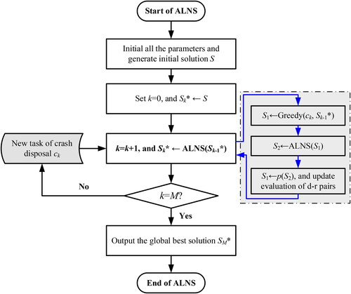
Figure 1 illustrates the overall flow of the ALNS algorithm. First, parameter initialization, including the number of RPVs, the status of RPVs, the positions of RPVs, and the start time, is shown. Then, a new task (i.e., crashes) is assigned, and the new optimal solution can be generated based on the initial or previous optimal solution. This process is iterative until all tasks are assigned, and the optimal global solution is obtained.

Figure 1. Flowchart of the ALNS algorithm.

(2) Self-adaptive weight adjustment strategy

To explore the appropriate strategy pair, the self-adaptive weight adjustment strategy was applied in this study. The selection probability of the strategy pair can be calculated by (21) $${\rho }_{\mathit{\text{dr}}}=\frac{{\omega }_{\mathit{\text{dr}}}}{\sum _{d=1}^{{\eta }_d}\sum _{r=1}^{{\eta }_r}{\omega }_{\mathit{\text{dr}}}}$$(21)

The search process is divided into several segments, each of which consists of φ successive iterations. The weight ω_dr and score π_dr will be assigned to each pair (d, r). Notably, the weights can be updated by the score accordingly. (22) $${\omega }_{\mathit{\text{dr}}}=\left\{\begin{array}{ll}\rho \frac{{\pi }_{\mathit{\text{dr}}}}{{o^{\prime }}_{\partial \mathit{\text{dr}}}{o^{\prime }}_{}}+\left(1-\rho \right){\omega }_{\mathit{\text{dr}}},\hfill & o^i{}_{\mathit{\text{dr}}}>0\hfill \\ {\omega }_{\mathit{\text{dr}}},\hfill & o^i{}_{\mathit{\text{dr}}}=0\hfill \end{array}\right.$$(22)

The weights of all strategy pairs in the initial stage are set to 1, and the scores are initially 0. After selecting the strategy pair in each iteration, if the new solution outperforms the original, the score of the strategy pair increases σ1; if the new solution is the optimal global solution, the score of the policy pair increases σ2; if no better solution is generated, however, the new solution is still accepted, and the score of the strategy pair increases σ3. In summary, it can be found that σ3<σ2<σ1.

(3) Delete-repair strategy pair

The deletion strategy is used to find new solutions in this study. Specifically, the successfully assigned tasks in the solution will be deleted and then reassigned to the repair program. Four deletion strategies were considered.

1. Random deletion strategy

   The random deletion strategy randomly selects 1-3 tasks in the solution sequence to delete, and the deleted tasks will be inserted into new positions in the subsequent repair program to generate new solutions. The utility performance of the newly generated solution cannot be guaranteed to be better than that of the original.

   This strategy can help to jump out of local optimal solutions. It does not need to calculate the disposal utility (i.e., the waiting time) of any task, and tasks will be directly deleted by a random selection procedure. However, the quality of the newly generated solution is unstable.

2. Worst-case deletion strategy

   After calculating the utility performance (such as the longest actual waiting time) of each task in the solution sequence, the worst deletion strategy selects 1-3 tasks with the worst utility to delete. The deleted tasks will be inserted into new positions in the subsequent repair program to generate new solutions. The utility performance of the newly generated solution will be more likely to be better than that of the original.

   This strategy can delete the tasks with the worst utility (the wait time, for instance) performance and will help to find a better disposal order in the subsequent repair strategy to obtain a better solution.

3. Distance deletion strategy

   After calculating the riding distances between tasks in the solution sequence, the distance deletion strategy selects 1-3 tasks with the largest riding distance to delete. The deleted tasks will be inserted into new positions in the subsequent repair program to generate new solutions. The utility performance of the newly generated solution will be better than that of the original solution at a certain probability.

   This strategy can help to reduce the travel time of RPVs. For instance, it can delete the tasks with the longest driving distance from their previous task of an RPV and will help to assign them to another closer RPV in the subsequent repair strategy.

4. Idle deletion strategy

   After calculating the idle time of the RPV assigned before the start of each task in the solution sequence, the idle deletion strategy selects 1-3 tasks with the largest idle time to delete. The deleted tasks will be inserted into new positions in the subsequent repair program to generate new solutions. The utility performance of the newly generated solution will be better than that of the original solution at a certain probability.

   To improve the efficiency of RPVs, an idle deletion strategy will be applied. This strategy will delete the tasks with the longest idle time from their previous task of an RPV and will help to assign them to another more appropriate RPV in the subsequent repair strategy.

Afterward, the repair strategy, including the greedy repair strategy and regret insertion strategy, is applied to repair the solutions by filling the deleted tasks into the current task chain of RPVs. The repair sequence can be determined according to the time of the deleted tasks. If the maximum waiting time constraint cannot be met during the repair process, the number of RPVs will be increased. In contrast, if there are idle RPVs after the repair process, the number of RPVs will be reduced accordingly.

1. Greedy repair strategy

The greedy repair strategy calculates the total waiting time increment of each RPV when inserting a new task into the task chain of the RPVs and chooses the RPV with the smallest waiting time increment.

1. Regret insertion strategy

The regret insertion strategy is designed based on the regret value of task insertion. It will calculate the total waiting time increment of each RPV after the task is inserted and choose the smaller of the largest intervals.

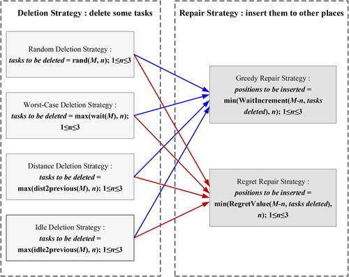
In total, there are eight ‘delete-repair’ strategy pairs. Detailed information is shown in Figure 2.

Figure 2. Combinations of the delete-repair strategy pairs.

(4) Evaluation of feasible solutions

The increase and decrease mechanism of the number of RPVs in the ALNS algorithm can ensure the feasibility of the generated solution. It is crucial to comprehensively evaluate these solutions because of the double objective functions of the model. (23) $$E=\alpha \frac{\mathrm{\text{max}}\hspace{0.17em}(Z)-Z}{\mathrm{\text{max}}\hspace{0.17em}(Z)-\mathrm{\text{min}}\hspace{0.17em}(Z)}+(1-\alpha )\frac{\mathrm{\text{max}}\hspace{0.17em}(F)-F}{\mathrm{\text{max}}\hspace{0.17em}(F)-\mathrm{\text{min}}\hspace{0.17em}(F)}$$(23)

In Constraint (23), $Z$ denotes the total waiting time of all crashes, and $F$ is the number of RPVs; $\mathrm{\text{min}}(Z)$ and $\mathrm{\text{max}}(Z)$ represent the minimum value and the maximum value of the total waiting time of all crashes at the optimal value, respectively; $\mathrm{\text{min}}(F)$ and $\mathrm{\text{max}}(F)$ represent the minimum value and the maximum value of the number of RPVs at the optimal value, respectively. Furthermore, the Dijkstra algorithm is applied to search for the optimal route between the tasks and RPVs.

Case study

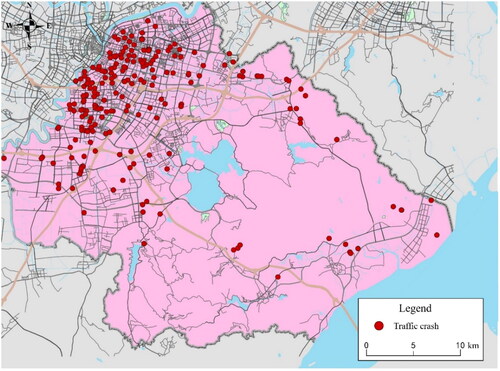
The study area is the Yinzhou District, Ningbo, China. The geographical area was 799.09 square kilometers. There are 8 traffic police stations in the region, the distribution of which is shown in Figure 3. The initial locations of RPVs are located at their respective traffic police stations. When a traffic crash disposal task is received, the RPV will depart from its initial location and return to this initial location after completing its full-day tasks. Crash data were collected from the Police Brigade in the Yinzhou branch of the Ningbo Public Security Bureau. Each record includes the crash location, occurrence time, crash types, weather conditions, and environment, including whether the light is sufficient and whether greening blocks vision. A total of 221 crash records were selected on July 22, 2020. The distribution of the crash data is shown in Figure 4.

Figure 3. Distribution of the traffic police stations.

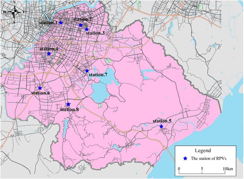
Figure 4. Distribution of the crash data.

Two methods, real-time dynamic resolution and global static resolution, were applied for case-solving in this study. The former indicates that RPVs do not know the finish time when handling the crash, and new tasks can only be assigned to idle RPVs. In contrast, the task finish time is primarily known in the latter, and the task reassignment evaluation can be done after full-day tasks.

The formulations of the methods mentioned above are specified as follows.

1. The real-time dynamic resolution method (24) $$x_{\mathit{\text{mn}}}=\left\{\begin{array}{ll}1,\hfill & \mathit{\text{if}}\hspace{0.17em}{p}_m\le e_{(q_{\mathit{\text{mn}}}\left(k\right)-1)}\hspace{0.17em}\mathit{\text{and}}\hspace{0.17em}{e}_{(q_{\mathit{\text{mn}}}\left(k\right)-1)}+t_{\mathit{\text{mn}}}\left(k\right)-p_m\le l_m\hfill \\ 0,\hfill & \mathit{\text{else}}\hfill \end{array}\right.$$(24)

2. The global static resolution method (25) $$x_{\mathit{\text{mn}}}=\left\{\begin{array}{ll}1,\hfill & \mathit{\text{if}}\hspace{0.17em}{e}_{(q_{\mathit{\text{mn}}}\left(k\right)-1)}+t_{\mathit{\text{mn}}}\left(k\right)-p_m\le l_m\hfill \\ 0,\hfill & \mathit{\text{else}}\hspace{0.17em}\hfill \end{array}\right.$$(25)

For the initial parameters of the ALNS-based algorithm, the number of RPVs was set to 10, the weight of the number of RPVs α was set to 0.3, the weight of the total waiting time of all the crashes was set to 0.7 and the scoring parameters of the ‘delete-repair’ strategy pairs were ${\sigma }_1=1.0$, ${\sigma }_2=0.4$, and ${\sigma }_3=0.25$, respectively.

Results of the real-time dynamic resolution

After task assignments are provided and dynamic searches are performed, the global optimal solution output by the ALNS algorithm under real-time dynamic resolution conditions is 13 RPVs. Information on the task lists is shown in Supplementary Table A1 (see in the Appendix). Also, some partially enlarged views of the riding routes of RPVs are shown in Figure 5.

Figure 5. Disposal task and riding route distribution under real-time dynamic solution conditions.

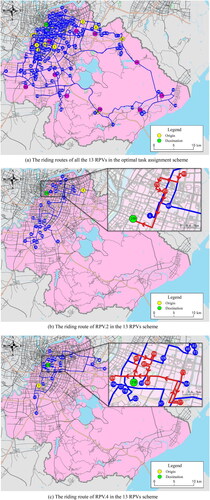
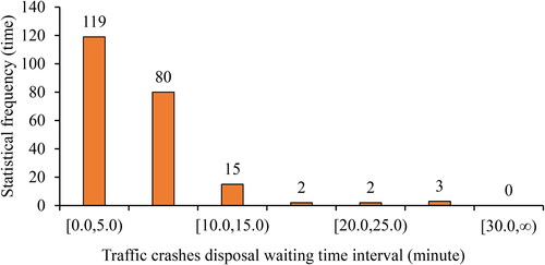
The total waiting time for all crashes is 1218.3 min, and the total travel time of all 13 RPVs is 1218.3 min. Figure 6 illustrates the distributions of the waiting times for crashes.

Figure 6. Distribution of the waiting time for crashes.

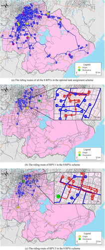
Results of the global static resolution

The results of the ALNS algorithm under global static resolution are shown in Figure 7 and Supplementary Table A2 (see in the Appendix). The results suggest that 8 RPVs can complete all tasks with a total travel time of 1,279.9 min.

Figure 7. Disposal task and riding route distribution under global static resolution conditions.

In addition, the time margins of RPVs, which represents the time difference between the former task being completed and the latter task starting, were calculated. (26) $$g_m=p_m-e_{{(q}_{\mathit{\text{mn}}}\left(k\right)-1)}$$(26)

The time margins of RPVs for the real-time dynamic solution and the global static solution are shown in Supplementary Table A3.

As shown in Supplementary Table A3, the number of RPVs using global static resolution is 8, the average waiting time of the crashes is 7.5 min, and the total time margin for crashes is 4079.3 min, significantly lower than the 7884.6 min of real-time dynamic resolution. This indicates that the RPV assignment for crashes is more accurate using the global static resolution, which can significantly reduce the time margin between tasks and, therefore, improve the efficiency of the RPV. However, the crashes’ total or average waiting time could be increased due to the time margins.

Discussion and conclusion

Discussion

(a) performance of the ALNS

To assess the performance of the ALNS, two other conventional algorithms were selected for model comparison, including the genetic algorithm (GA) and the ant colony algorithm (ACA). GA and ACA have no adjustment mechanism for the number of RPVs, so the two algorithms were used to solve the problem by specifying the number of RPVs in advance. The range of the number of RPVs was set as 6 to 20, and the optimal assignment of tasks was carried out in the real-time dynamic resolution mode and the global static resolution mode. The results are shown in Supplementary Table A4 (see in the Appendix).

In the real-time dynamic resolution mode, regardless of the GA or the ACA, within the set range of the number of RPVs, they failed to search for any feasible solution successfully. That is, they failed to make the actual waiting time of all tasks not exceed their maximum waiting time. GA or ACA is a static resolution algorithm. Moreover, assigning idle RPVs to sudden tasks only by cross/mutation operations or pheromone induction mechanisms is impossible under the condition of meeting the longest waiting time constraint. At the same time, it can be seen that the increase in the number of RPVs only reduced the actual waiting time of tasks by a small margin, indicating that the algorithms were trapped in the local optimum during iteration.

In the global static resolution mode, the performance of the GA and ACA were slightly better than in the real-time dynamic resolution mode. When there was 18 or 16 RPVs, a feasible solution satisfying the constraints could be found. However, compared with the optimal solution searched by ALNS, the actual waiting time was 59.5% larger, and the number of RPVs was 100% more. These results fully show that the mechanism setting of the ALNS algorithm is superior to that of the GA or ACA.

(b) sensitivity analysis

In this study, the proposed model has two objective functions, the minimum number of RPVs and the minimum waiting time to reach crashes. A sensitivity analysis was conducted to assess the robustness of the model.

The weight factor α varies in the range of [0.0, 1.0]. When α = 0.0, the model degenerates into a single objective optimization model with the minimum number of RPVs; when α = 1.0, the model degenerates into a single objective optimization model with the minimum total waiting time. Figure 8 shows the change in the number of RPVs and total waiting time with the weight factor α.

Figure 8. Influence of the α value on the feasible optimal solutions.

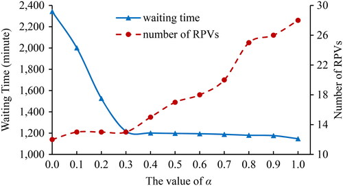
When α = 0.0, the number of RPVs is 12, and the total waiting time is 2343.0 min. There is no feasible solution when the number of RPVs is less than 12 since it is challenging to ensure that the actual waiting time for all crashes is less than the maximum waiting time. When α = 1.0, the number of RPVs is 28, and the total waiting time is 1147.6 min. In general, if the number of RPVs equals the number of crashes, the total waiting time should be 773.5 min when each RPV is only assigned to one crash. However, it is difficult to achieve such theoretical optimality in practice. This is mainly attributed to the greedy strategy for dynamic task allocation of the crash and the strategy design for the repair operation. When the number of RPVs exceeds 27, any deleted crash can find a suitable location that meets all constraints when repaired. Meanwhile, increasing the number of RPVs is not triggered indefinitely. When 0.0<α < 1.0, the results suggested that the number of RPVs could increase with the weight factor α, and the total waiting time shows a decreasing trend. In other words, the more RPVs are operated, the smaller the total waiting time.

Furthermore, we found that the total waiting time for crashes of 28 RPVs is not considerably lower than that of 13 RPVs. The waiting time for crashes in the task allocation scheme for 13 RPVs is equal to the travel time, which indicates that the crashes in the task chain of each RPV have a good aggregation in space-time under this allocation scheme. This finding also proves the efficiency of the task allocation scheme for 13 RPVs.

Conclusion

In this paper, the imbalance issue between limited police resource allocations and the timely handling of road traffic crashes is emphasized. A dynamic crash-handling response model was developed to optimize resource allocations and route choices for RPV assignments. Specifically, two objective functions were designed: the minimum waiting time and the minimum number of RPVs. In particular, two resolution methods, real-time dynamic resolution, and global static resolution mode, were applied to explore the optimal solutions based on comprehensive traffic and crash data in Ningbo, China. The research summary is as follows.

1. The optimal allocation scheme for the traffic police is 13 RPVS using the real-time dynamic resolution. For instance, the average waiting time to reach crashes is 5.5 minutes, with 53.8% of crashes being reached in less than 5 minutes and 90.0% in less than 10 minutes.

2. If only considering the minimum number of RPVs, the optimal allocation scheme for the traffic police is 12 RPVs, and the total waiting time of all crashes is 2343.0 minutes. If the number of RPVs is less than 12, the model has no feasible solution. In contrast, the optimal allocation scheme for the traffic police is 28 RPVs if only considering the minimum waiting time for all crashes. In addition, the algorithm is able to avoid converging to a theoretically optimal allocation without practical significance due to the greedy strategy and the repair strategy design.

The findings of this study are expected to provide insightful instruction for road safety management. For instance, the proposed method can be indicative of the RPV allocation scheme for the disposal of crashes and, therefore, improve road safety in the long run. However, there are still some limitations in the current study. For instance, the matching rule of RPVs and crashes is too strong. In practice, the system will assign an RPV to emergency crashes, although they are possibly handling other crashes. However, this practical rule could put forward higher requirements for the optimization mechanism of the proposed model. In the future, more consideration will be given to some complex scenarios to improve the performance of the proposed algorithm.

Disclosure statement

No potential conflict of interest was reported by the author(s).

Additional information

Funding

This study was supported by National Natural Science Foundation of China (No. 52002282), Basic Public Welfare Research Project of Zhejiang Province (LGF20F030004). Also, we are grateful to thank Dr. Jiyan Wu from Tongji University and Dr. Xinhua Mao from Chang’an University for their contributions to the problem description and solving algorithms.

References

- Adulyasak Y, Cordeau JF, Jans R. 2014. Optimization-based adaptive large neighborhood search for the production routing problem. Transport Sci. 48(1):20–45. doi:10.1287/trsc.1120.0443.
- Ahmad M, Jayalalitha G. 2021. A reverse reneging queuing model for single server with finite capacity model. Design Engineering. 1(8):12683–12687.
- Aiello MF. 2021. Procedural justice and demographic diversity: a quasi-experimental study of police recruitment. Police Q.; 25(3):387–411. doi:10.1177/10986111211043473.
- Archetti C, Speranza MG, Boccia M, Sforza A, Sterle C. 2020. A branch-and-cut algorithm for the inventory routing problem with pickups and deliveries. Eur J Oper Res. 282(3):886–895. doi:10.1016/j.ejor.2019.09.056.
- Azi N, Gendreau M, Potvin JY. 2014. An adaptive large neighborhood search for a vehicle routing problem with multiple routes. Comput Oper Res. 41:167–173. doi:10.1016/j.cor.2013.08.016.
- Dayarian I, Crainic TG, Gendreau M, Rei W. 2016. An adaptive large-neighborhood search heuristic for a multi-period vehicle routing problem. Transport Res E-Log. 95:95–123. doi:10.1016/j.tre.2016.09.004.
- Ding HL, Lu YH, Sze NN, Antoniou C, Guo YY. 2023. A crash feature-based allocation method for boundary crash problem in spatial analysis of bicycle crashes. Anal Methods Accid R. 37:100251. doi:10.1016/j.amar.2022.100251.
- Ding HL, Lu YH, Sze NN, Chen TT, Guo YY, Lin QH. 2022. A deep generative approach for crash frequency model with heterogeneous imbalanced data. Anal Methods Accid R. 34:100212. doi:10.1016/j.amar.2022.100212.
- Heyer GD, Mitchell M, Ganesh S, Devery C. 2008. An econometric method of allocating police resources. Int J Police Sci Manag. 10(2):192–213. doi:10.1350/ijps.2008.10.2.74.
- Ho LKK. 2020. Rethinking police legitimacy in postcolonial Hong Kong: paramilitary policing in protest management. Polic-J Policy Pract. 14(4):1015–1033. doi:10.1093/police/paaa064.
- Hoque Z, Arends S, Alexander R. 2004. Policing the police service: a case study of the rise of “new public management” within an Australian police service. Acc Audit Account J.17(1):59–84. doi:10.1108/09513570410525210.
- Hu HT, Mo J, Zhen L. 2021. Improved benders decomposition for stochastic yard template planning in container terminals. Transport Res C-Emer. 132(8):103365. doi:10.1016/j.trc.2021.103365.
- Jagat SS. 2021. The role of Bhabinkamtibmas through counseling guidance in preventing crime of theft with aggravated circumstances in the legal territory of the Klaten Police. Adv. Police Sci. Research J. 5(11):1–8. https://garuda.kemdikbud.go.id/documents/detail/2507991.
- Kolesar PJ, Rider KL, Crabill TB, Walker WE. 1975. A queuing-linear programming approach to scheduling police patrol cars. Oper Res. 23(6):1045–1062. doi:10.1287/opre.23.6.1045.
- Koskey MC, Njoroge J. 2019. Influence of employee retention practices on employee performance in disciplined services: case of the administration police service Nyandarua County, Kenya. IJCAB. 3(III):83–95. doi:10.35942/ijcab.v3iIII.32.
- Kovacs AA, Parragh SN, Doerner KF, Hartl RF. 2012. Adaptive large neighborhood search for service technician routing and scheduling problems. J Sched. 15(5):579–600. doi:10.1007/s10951-011-0246-9.
- Krukowski K, Siemiński M. 2018. New public management in organisations introducing agricultural policies in Poland. Manag Theory Stud Ru. 40(2):206–215. doi:10.15544/mts.2018.20.
- Li JT, Zhao Z. 2022. Impact of COVID-19 travel-restriction policies on road traffic accident patterns with emphasis on cyclists: a case study of New York City. Accid Anal Prev. 167:106586. doi:10.1016/j.aap.2022.106586. PMID: 35131653.
- Li J-Q, Han Y-Q, Duan P-Y, Han Y-Y, Niu B, Li C-D, Zheng Z-X, Liu Y-P 2020. Meta-heuristic algorithm for solving vehicle routing problems with time windows and synchronized visit constraints in prefabricated systems. J Cleaner Prod. 250:119464. doi:10.1016/j.jclepro.2019.119464.
- Liu JH, Yang JG, Liu HP, Tian XJ, Gao M. 2017. An improved ant colony algorithm for robot path planning. Soft Comput. 21(19):5829–5839. doi:10.1007/s00500-016-2161-7.
- Luan YP, Ye SL, Li YM, Jia L, Yue XG. 2022. Revisiting natural resources volatility via TGARCH and EGARCH. Resour Policy. 78:102896. doi:10.1016/j.resourpol.2022.102896.
- McIlroy RC, Plant KA, Hoque MS, Wu J, Kokwaro GO, Nam VH, Stanton NA. 2019. Who is responsible for global road safety? A cross-cultural comparison of Actor Maps. Accid Anal Prev. 122:8–18. doi:10.1016/j.aap.2018.09.011. PMID: 30300797.
- Munyeka W, Setati TS. 2022. Organisational politics on job satisfaction: an empirical study of police officials in a selected police service station. Afr Public Serv Deliv Perform Rev. 10(1):1–10. doi:10.4102/apsdpr.v10i1.552.
- Nepomuceno TC, Daraio C, Costa APCS. 2021. Multicriteria ranking for the efficient and effective assessment of police departments. Sustainability. 13(8):4251. doi:10.3390/su13084251.
- Peng KK, Gao MX, Chen HJ, Tang JY, Xing YQ, Jiang F. 2023. Rural policing in China: criminal investigation and policing resources for police officers. Heliyon. 9(8):e18934. doi:10.1016/j.heliyon.2023.e18934.PMID: 37600418.
- Sacks SR. 2000. Optimal spatial deployment of police patrol cars. Soc Sci Comput Rev. 18(1):40–55. doi:10.1177/089443930001800103.
- Sayarshad HR. 2022. Designing an intelligent emergency response system to minimize the impacts of traffic incidents: a new approximation queuing model. Int J Urban Sci. ; 26(4):691–709. doi:10.1080/12265934.2022.2044890.
- Tamannaei M, Irandoost I. 2019. Carpooling problem: a new mathematical model, branch-and-bound, and heuristic beam search algorithm. J Intell Transport S. 23(3):203–215. doi:10.1080/15472450.2018.1484739.
- Terpstra J, Schaap D. 2021. The politics of higher police education: an international comparative perspective. Polic-J Policy Pract. 15(4):2407–2418. doi:10.1093/police/paab050.
- Wang DY, Liu QY, Ma L, Zhang YJ, Cong HZ. 2019. Road traffic accident severity analysis: a census-based study in China. J Safety Res. ; 70:135–147. doi:10.1016/j.jsr.2019.06.002. PMID: 31847989.
- Wong GTW, Manning M. 2022. Enhancing police efficiency in detecting crime in Hong Kong. Crime Law Soc Change. 78(3):321–355. doi:10.1007/s10611-022-10027-0.
- World Health Organization. 2019. Global status report on alcohol and health 2018. Geneva (Switzerland): World Health Organization.