Vehicle and twin-roller chassis dynamometer model considering slip tire interactions

Abstract

xComputational representation of real-world systems plays an important role in vehicle analysis. Aiming to improve mobility systems, this article presents the development of a chassis dynamometer and vehicle model describing the vehicle longitudinal dynamics considering the tire-bench contact. The model simulates the longitudinal vehicle-bench tests where the system is powered by the bench’s electric motor and the gearbox in the neutral position, considering tire interaction forces, rolling resistance, and system losses. It was implemented in Matlab/Simulink™ and validated by coast-down experiments, starting at 60 km/h and 100 km/h, where the model result curves presented an appropriated representativity for the experimental data. A total movement resistance analysis resulted in a mean error of 6.71% when compared to experimental data, while the literature slip-independent equations presented mean errors between 31.94% and 77.61%. The developed model is a representative approximation of the vehicle-dynamometer set and can predict longitudinal experiments, helping the vehicle evaluation process, and saving time and resources.

Keywords:

• Vehicle simulation
• chassis dynamometer
• vehicle dynamics
• experimental validation

1. Introduction

Vehicles are present in daily life, mainly in big cities (Miranda et al. 2022), and are probably the prominent fossil fuel consumers (Delkhosh, Foumani, and Boroushaki 2014; Eckert et al. 2022). In order to make the mobility systems more efficient, these vehicles need constant improvement and evaluation aiming to fit the drivers’ necessities and government regulations (Dong et al. 2020; Aldy et al. 2021). To achieve these goals, vehicle manufacturers need to provide fast technological changes as the use of alternative fuels/power sources (Roso et al. 2019; Barbosa et al. 2020; Silva, Eckert, Lourenço, et al. 2021), lighter materials to minimize vehicle weight (enhance fuel efficiency) (Ghadge and Prakash 2021), and enhanced control techniques (Eckert, Bertoti, et al. 2021; Silva, Eckert, Lourenço, et al. 2021) which need to be experimentally evaluated before reaching the vehicle market (Habermehl, Jacobs, and Neumann 2020). Vehicles are submitted to different indoor tests under standard and eventually severe scenarios, evaluating powertrain changes according to extreme environmental conditions as high altitudes, aggressive climbs, different barometric pressures, temperatures gradients, and humidity levels (Bielaczyc, Woodburn, and Szczotka 2016; Lohse-Busch et al. 2020). Nowadays, with the Covid pandemic closing boards and limiting world travels, more than ever, there is a hurry for alternative testing solutions, and these solutions are commercial and engineering appealing, even in a Covid-free world.

One of the main testing vehicle platforms is a chassis dynamometer (Eckert et al. 2017), also known as roller dynamometer and automotive dynamometer bench. There are two main types of chassis dynamometer: single-roller type and twin-roller type (Silva et al. 2016). Therefore, there are different tire contact configurations and footprint, depending on the number of rollers (Silva et al. 2016). This equipment enables to carry out analyses such as durability, fuel consumption, emissions, engine performance, global and component efficiencies, emulation of standardized cycles and of external conditions (Lairenlakpam, Kumar, and Thakre 2019; Jouanne et al. 2020), and so on. In addition, this type of platform provides reliable and controlled experimental conditions, used by the automotive industry in the development of new technologies, since they are capable of simulating real conditions and can be controlled by a computer (Wager et al., 2014). When compared to a vehicle test on the road, tests on chassis dynamometers are less expensive and more effective to obtain characteristic data with precision, being also applied in academic research, allowing to reproduce test (Eckert et al. 2017; Bertoti et al. 2019).

Several works have used this type of platform to analyze vehicles for different purposes, such as validation of energy management strategies for Electric Vehicles (EVs) (Song et al. 2018) and Hybrids Electric Vehicles (HEVs) (Mayyas et al. 2017; Eckert et al. 2019), validation of hybrid engines (Mayyas et al. 2017), evaluation of the effect of the transmission gears of combustion vehicles converted to EV (Wager et al., 2014), verification of effects of gear shifting strategies in acceleration performance and fuel consumption (Eckert, Bertoti, et al. 2021), forecast of energy consumption for urban electric buses (Beckers et al. 2019), automation of steering test of manual transmission vehicles (Euler-Rolle et al., 2020), execution of indoor noise test with a set of microphones around the chassis dynamometer (Chen et al. 2021) and inside the vehicle cabin (Kim et al. 2013), verification of the performance of longitudinal force observers in EVs (Chen et al. 2018), validation of the vibration and noise of automotive powertrain mounting systems (Shangguan et al. 2016) among other examples. Therefore, based on recent research, the applicability and importance of this equipment are shown.

Vehicles on the dynamometer bench can be submitted to more severe movement resistances, hence, more power is demanded when compared to a real-world application (Eckert et al. 2017). Moreover, at the bench, the tire footprint is curved and it alters the contact pressure distribution (Silva et al. 2016). Also, it is well-established that tire and roller contact, specially in twin-roller dynamometers, is an important issue when characterizing the vehicle dynamic behavior, a key factor in design control, hence, extremely relevant in vehicle dynamic simulation models (Silva et al. 2016). Thereby, for chassis benches, the tire contact on the bench needs to be analyzed, which differs from the standard tire contact with a plane floor/ground. Table 1 brings the most relevant dynamometer bench tire contact researches.

Table 1. Tire contact analyses in dynamometer benches.

References	Details
Eckert et al. (2017)	Empirical definition of the inertia of a roller dynamometer, as well as its torque losses. It is also shown how to evaluate the tire rolling resistance in this facility.
Pałasz et al. (2019)	Tire rolling resistance coefficients using a roller dynamometer and comparison with the ones available at the literature.
Ejsmont and Owczarzak (2019)	Developement of a test rig (with exchangeable contact surface) to access the so-called coefficient of energy losses. It was verified the correlation between this coefficient and the rolling resistance coefficient.
Pexa et al. (2020)	Measurement of the rolling resistance on roller dynamometers considering a large set of roller sizes, vertical loads, speeds and inflation pressures. The results showed the variation of the roller size has a greater impact on the measured rolling resistance.
Soica et al. (2020)	A method for obtaining the tire rolling resistance coefficients from tests at roller dynamometers. The results are validated by means of coefficients generated from drum tests.
Martyr and Plint (2012)	Model of a single roller dynamometer tire contact force and rolling resistance as a function of tire and roller radii ratio and speed-dependent coefficients.

Although Table 1 shows notable works, among experimental identifications and well-established equation modeling, researches have been performed and shown the literature does not present a detailed analysis of the vehicle-dynamometer interaction, mainly focused on the tire-rollers contact. No studies showed the effects of vehicle-bench slip and resistance coefficients, principally to a twin-roller contact type of chassis dynamometer. Since there are no tire-roller models considering the slip effects, it is necessary to adapt the existing tire-ground models to the twin-roller contact. There are several tire contact models (Alcazar et al. 2020), among these, the some are briefly presented in Table 2.

Table 2. Tire models for tire-ground contact.

References	Details
O’Neill et al. (2021)	Brush tire model enhancement through a simpler approach considering friction measurements.
Salehi et al. (2021)	Analysis of the interface of a rolling rubber wheel on a counter-surface disk under a tribological aspect.
Salehi et al. (2020)	Prediction of tire grip with a Laboratory Abrasion Tester as a tribometer.
Pacejka (2012)	Tire dynamics with empirical tire models considering slipping situation, widely known as Magic Formula, with different versions improved over the years.
Besselink, Schmeitz, and Pacejka (2010)	Extensions of the Magic Formula, including inflation pressure and large camber angles.
Gao et al. (2021)	Tire rolling deformation with flexible ring tire model extended with dynamic pressure distribution under high-speed rolling condition.

Among the well-established studies about tires, the main empirical tire model, has been ultimately described by Pacejka (2012), with the first model dating from 1987 and with different updated versions published over the years. The recent version was updated to support uneven roads and extreme camber angles. Many researchers have presented works based on Pacejka’s approach, as seen in Table 2. One of these is the work proposed by Besselink, Schmeitz, and Pacejka (2010), who presented an improvement of Pacejka’s Magic Formula tire model, being able to handle changes of inflation pressure. One recent work was shown by O’Neill et al. (2021), where a physical-based brush-type tire model was proposed aiming to achieve tire behavior results similar to Pacejka’s model, but using a simpler approach and considering rubber friction characteristics. Salehi et al. (2020) also analyzed tires and developed a rapid test method to predict tire grip in a laboratory. In later work, Salehi et al. (2021) showed a tribological view of the interface of a rolling rubber wheel on a counter-surface disk, correlating tire grip and laboratory-road with modeling. Moreover, Gao et al. (2021) described the modeling and experiments of tire deformation in high-speed scenarios, considering dynamic pressure distribution and the flexible ring tire model. On the other hand, computational tire models are also commonly used. The main finite elements and shell elements tire models, respectively FTire and CDTire, predict the contact with a single inner or outer drum. However, the contact with twin-rollers has not been explored by these models until now.

This way, since there are no detailed tire-roller models, this article considers an adaptation of the Pacejka tire model (detailed in section 3.1), due to its recurrent use in vehicle analyses and its larger database with more available information from different tires (ADAMS 2019). Thus, it is possible to select a tire, and its parameters, closer as possible to the real one used in the experiment, leading to more accurate results.

Moreover, the computational representation of real-world systems plays an important role in vehicle analysis and has been applied in many recent works (Pan et al. 2020), since it is an important tool for evaluating critical conditions (Eckert, Bertoti, et al. 2021). In real-case scenarios, the developed model allows reducing test time, once it is possible to carry out virtual experiments before the real ones, helping the vehicle evaluation process in order to attend regulations and drivers’ necessities. Therefore, with the virtual model, it is possible to first evaluate hypotheses virtually, reducing the real tests, helping to indicate the promising experiments which worthy to be validated with the physical bench infrastructure. By reducing the usage of physical infrastructure, it is possible to save resources, once the real experimental set needs monitoring rooms, exhaust system, compressed air lines, maneuver spaces, which implies high costs (Fajri et al. 2016). Also, the applied simulation techniques lower the necessity of prototype vehicles (Aceituno et al. 2017).

Besides, the existent commercial softwares are not capable of simulating the dynamometer with the interactions of the double contact between the tire and the rollers, but only vehicles in different road situations in a single tire contact. On the other hand, laboratory chassis dynamometers are widely applied in vehicles’ regulatory standards, such as in 10521-2:2006(E) (2006) (Road vehicles – Road load – Part 2: Reproduction on chassis dynamometer), 28981:2009(E) (2009) (Methods for setting the running resistance on a chassis dynamometer), NBR10312 (2014) (Light duty road vehicles—Road load measurement and dynamometer simulation using coast-down techniques). Thus, despite the existing softwares’ contribution with different tire-surface simulations, they are not able to reproduce the double contact of chassis dynamometer tests, an essential feature of these experiments performed in the vehicle homologation process. Therefore, simulating laboratory tests on chassis dynamometers, even though they do not replace tests on real benches, reduces the number of required tests by performing virtual tests, contributing to minimizing the time spent and overall costs, accelerating the homologation process.

Based on the large literature review performed (as presented by Tables 1 and 2), works showing the development of a vehicle-dynamometer model, detailing the interaction contact forces, were not found. This article proposes the development of a dynamometer-vehicle model of a twin-roller chassis dynamometer placed at the Integrated Systems Laboratory (LabSIn) at the University of Campinas (São Paulo state - Brazil). The developed model details the tire-bench double contact interaction, considering slip, rolling resistance, and system longitudinal dynamic behavior, and also reuniting the consolidated and experimentally validated theories. This approach unites simulation techniques, control strategies, experimental data, conceptual and experimental models, allowing a more accurate and complete representation of the real system, not found in the literature for a vehicle-dynamometer application.

The analysis proposed in this article focuses on reproducing coast-down and total bench resistance tests, as well as analyzing the slip tire-rollers interactions in these scenarios, in order to calibrate and validate the developed vehicle-bench model to be as representative as possible to the real loads in a laboratory experiment. The model considers the longitudinal vehicle-bench dynamics and in all simulated tests, the system is powered by the bench’s electric motor with the vehicle gearbox in the neutral position, where the vehicle does not provide power. Besides, it is important to highlight that in the simulated experiments there is no action from the vehicle breaks and the lateral and vertical dynamics, such as turning maneuvers and vehicle suspensions, respectively, are disregarded. Thus, with a representative model of the vehicle-bench longitudinal resistance loads, in future work will be possible to add vehicle powertrain characteristics aiming to pre-run other virtual experiments, such as driving cycles analysis under different acceleration and braking situations.

In order to achieve this goal, the Section 2 presents the real dynamometric bench taken into account in this article and its main features. Then, the vehicle-bench interaction loads are introduced in Section 3 aiming to support the logic developed in the simulation model described in Section 4, also presenting the simulation parameters. After applying the model, the achieved results are analyzed in Section 5. Finally, Section 6 brings an overview of the main contributions of this article and the research future perspectives.

2. Labsin’s Chassis dynamometer bench

The reference bench used in this work is a chassis dynamometer, also known as a twin-roller dynamometer, and it is located in the Integrated Systems Laboratory at the University of Campinas (Brazil). This bench has been improved over the years to allow different analyses (Eckert et al. 2017). Figure 1(a) shows a picture of the bench setup, where the vehicle considered is the FIAT${}^{TM}$ Punto 2008 1.4 L.

Figure 1. LabSIn’s chassis dynamometer bench.

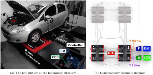
As seen in Figure 1(a), this bench has two actuators: an Electric Motor (EM) and an Eddy Current Brake (ECB) connected to the axles of the frontal rollers. This feature emulates external effects by adding or minimizing system loads. Besides, reducers were positioned between the actuators and the rollers to amplify the torque provided by both the EM and the ECB (Bertoti et al. 2019). A more detailed view is presented in Figure 1(b) with an assembly diagram of the main components, also indicating the Internal Combustion Engine (ICE), the rollers numbers (1, 2, 3, and 4), the two torque measurements points T (500 Nm and 3 kNm), and the reduction R and the planetary gearbox P in order to increase the final torque available and provide better-operating regimes for both systems. This study considers only front-wheel driving vehicles.

3. Vehicle-bench loads

To model the vehicle behavior, firstly, it is necessary to understand vehicle dynamics basic concepts. Subsection 3.1 describes the tire slip model considered and how it is adapted to twin-roller tire contact. Then, the rolling resistance concepts are introduced in Subsection 3.2, highlighting the slip-dependent approach. The empirical systems losses are also included in the model, as presented in Subsection 3.3. The resultant loads acting on the components are presented in Subsection 3.4. It is important to highlight the model considers only the longitudinal dynamics (lateral and vertical dynamics are disregarded) and for the simulated experiments, there is no power or breaking coming from the vehicle, the gearbox stays in neutral, and the setup is powered by the EM from the bench.

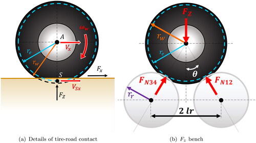
For the analysis proposed in this article, Pacejka model, detailed in the following, was chosen due to its accuracy in describing tire-ground slip behavior, once the equations are fitted to several experimental data. Nowadays, Pacejka models are considered state-of-the-art for modeling tire-road interaction forces (ADAMS 2019). Besides, the tire footprint and pressure distribution are different from the ground standard case and the Pacejka model dependency on the normal force allows it to be adjusted to the tire-rollers case through the contact angle θ, as seen in Figure 2(b), and detailed in the following section.

Figure 2. Slip tire details.

3.1. Pacejka Magic Formula

For a more accurate vehicle-bench dynamics model, the representation of tire-road interaction forces is inevitable, once the movements primarily depend on the road forces on the tires (ADAMS 2019). Pacejka (2012) proposed empirical tire models able to adapt to the behavior of the forces and moments present in a slipping situation, being an excellent approximation (Genta and Morello 2009). The main versions of this model were launched in 1989, 1994, and 2002.

Figure 2(a) presents the main reference points for wheel movement, where A is the wheel center, S is the slip point, V_x (m/s) is the longitudinal speed of the wheel center, ω_w (rad/s) is the wheel rotation, F_x (N) is the Pacejka longitudinal force, F_z (N) is the vertical force acting on the tire, and r_w (m) and r_e (m) are, respectively, the radius of the non-deformed tire and the effective radius (calculated based on 98% of the non-deformed radius r_w [m] Genta and Morello (2009)). V_Sx (m/s) is the relative slip speed defined in Eq. (1)(1) $$V_{Sx}=V_x-V_w$$(1) as the difference between V_x and the wheel tangential speed V_w, as shown in Eq. (2)(2) $$V_w=r_e·{\omega }_w$$(2) , as a function of r_e and ω_w. (1) $$V_{Sx}=V_x-V_w$$(1) (2) $$V_w=r_e·{\omega }_w$$(2)

For the dynamometer double contact, the normal forces$F_{N12}$ and $F_{N34}$ acting at the tire are shown in Figure 2(b), where θ is the angle between the vertical axis and the wheel-roller centerline. These forces are a function of the system geometry, as the roller radius r_r, the r_e, and the horizontal distance between the roller and the wheel center lr (m), as presented in Eq. (3)(3) $$F_N=\frac{F_z}{2}\frac{r_r+r_e}{\sqrt{{(r_r+r_e)}^2-l{r}^2}}$$(3) . (3) $$F_N=\frac{F_z}{2}\frac{r_r+r_e}{\sqrt{{(r_r+r_e)}^2-l{r}^2}}$$(3)

The tire slip κ is calculated as the ratio between V_Sx and V_x, as shown in Eq. (4)(4) $$\kappa =-\frac{V_{Sx}}{V_x}$$(4) . (4) $$\kappa =-\frac{V_{Sx}}{V_x}$$(4)

The longitudinal slip is null for a free-rolling wheel when S has no speed and becomes the wheel instant center of rotation. At braking, where V_Sx is positive, the slip κ is negative. On the other hand, κ is positive during traction. Once the slip is calculated, the longitudinal force F_x (N) is obtained as in Eq. (5)(5) $$F_x=D_x\hspace{0.17em}\mathit{\text{sin}}[C_{x}ta{n}^{-1}(B_x{\kappa }_x-E_x(B_x{\kappa }_x-ta{n}^{-1}(B_x{\kappa }_x)))]+S_{vx}$$(5) , also known as Magic Formula (MF). Pacejka developed equations for longitudinal, lateral and momentum cases. In this article, the approach considers only the vehicle longitudinal dynamics. (5) $$F_x=D_x\hspace{0.17em}\mathit{\text{sin}}[C_{x}ta{n}^{-1}(B_x{\kappa }_x-E_x(B_x{\kappa }_x-ta{n}^{-1}(B_x{\kappa }_x)))]+S_{vx}$$(5) (6) $${\kappa }_x=\kappa +S_{Hx}$$(6)

Where S_Vx and S_Hx are the vertical and horizontal longitudinal increments, B_x is the stiffness factor, C_x is the form factor, D_x is the curve peak value, and E_x is the curvature factor (Pacejka 2012). These coefficients are calculated based on empirical parameters measured for each type of tire and they change according to the model version considered. Considering the 2002 MF version (Pacejka 2012; ADAMS 2019), the equations for the longitudinal case are presented as follows, where μ_x is the maximum friction coefficient, df_z is the normalized variation of the vertical load, and $F_{\text{nomin}}$ (N) is the nominal (rated) load. (7) $$d{f}_z=\frac{F_N-F_{\text{nomin}}}{F_N}$$(7) (8) $${\mu }_x=\left(p_{Dx1}+p_{Dx2}d{f}_z\right)\left(1-p_{Dx3}{\gamma }^2\right){\lambda }_{\mu x}$$(8) (9) $$D_x={\mu }_x{F}_N$$(9) (10) $$K_{x\kappa }=\left(p_{Kx1}+p_{Kx2}d{f}_z\right)e^{\left(p_{Kx3}d{f}_z\right)}{F}_N{\lambda }_{Kx\kappa }$$(10) (11) $$C_x=p_{Cx1}{\lambda }_{Cx}$$(11) (12) $$B_x=\frac{K_{x\kappa }}{C_x{D}_x}$$(12) (13) $$S_{Hx}=\left(p_{Hx1}+p_{Hx2}d{f}_z\right){\lambda }_{Hx}$$(13) (14) $$S_{Vx}=F_N\left(p_{Vx1}+p_{Vx2}d{f}_z\right){\lambda }_{Vx}{\lambda }_{\mu x}$$(14) (15) $$E_x=\left(p_{Ex1}+p_{Ex2}d{f}_z+p_{Ex3}d{f}_z^2\right)\left(1-p_{Ex4}s\mathit{ign}\left({\kappa }_x\right)\right){\lambda }_{Ex}$$(15)

Where γ is the camber angle (considered null in this analysis), ${\lambda }_{Fz0},{\lambda }_{\mu x},{\lambda }_{Kx\kappa },$ λ_Cx, λ_Ex, λ_Hx, and λ_Vx are scale factors (considered unitary for this approach), and $p_{Dx1},p_{Dx2},p_{Dx3},p_{Kx1},p_{Kx2},p_{Kx3},$ $p_{Cx1},p_{Ex1},p_{Ex2},p_{Ex3},p_{Ex4},p_{Hx1},$ $p_{Hx2},p_{Vx1},$ and $p_{Vx2}$ are the tire parameters experimentally measured. For this case, the parameters used are presented in Table 3 (ADAMS 2019).

Table 3. Pacejka longitudinal parameters (ADAMS 2019).

$p_{Dx1}$	$p_{Dx2}$	$p_{Dx3}$	$p_{Kx1}$	$p_{Kx2}$
1.1387	−0.11999	2.2142 $·$ 10^−5	18.886	−3.988
$p_{Kx3}$	$p_{Cx1}$	$p_{Ex1}$	$p_{Ex2}$	$p_{Ex3}$
0.21542	1.839	0.62727	−0.12336	−0.03448
$p_{Ex4}$	$p_{Hx1}$	$p_{Hx2}$	$p_{Vx1}$	$p_{Vx2}$
−1.5066 $·$10^−5	−3.3912 $·$10^−4	−8.5877 $6$10^−6	−4.638 $·$10^−6	1.9874 $·$10^−5

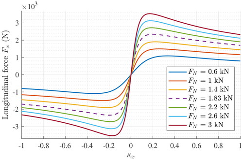
Applying these parameters in Eqs. (5)(5) $$F_x=D_x\hspace{0.17em}\mathit{\text{sin}}[C_{x}ta{n}^{-1}(B_x{\kappa }_x-E_x(B_x{\kappa }_x-ta{n}^{-1}(B_x{\kappa }_x)))]+S_{vx}$$(5) to (15)(15) $$E_x=\left(p_{Ex1}+p_{Ex2}d{f}_z+p_{Ex3}d{f}_z^2\right)\left(1-p_{Ex4}s\mathit{ign}\left({\kappa }_x\right)\right){\lambda }_{Ex}$$(15) and varying F_N and κ_x, it is possible to obtain the F_x curves presented in Figure 3, where the dashed curve (F_N = 1.83 kN) represents the longitudinal force for each tire-roller contact. It is noteworthy that for small slip values (modulus under 0.1), where most cases fit, the curves present approximately linear behavior and a major growth rate. After the peak is reached, F_x decays to a constant value while κ_x tends to infinity.

Figure 3. Pacejka longitudinal curves (2002 model) of the tire 195/65 R15 (ADAMS 2019).

Once the longitudinal force F_x is known by the Eq. (5)(5) $$F_x=D_x\hspace{0.17em}\mathit{\text{sin}}[C_{x}ta{n}^{-1}(B_x{\kappa }_x-E_x(B_x{\kappa }_x-ta{n}^{-1}(B_x{\kappa }_x)))]+S_{vx}$$(5) , the torque on the roller T_x is obtained as expressed in Eq. (16)(16) $$T_x=F_x{r}_r$$(16) , as a function of the roller radius r_r. (16) $$T_x=F_x{r}_r$$(16)

3.2. Rolling resistance

At low speeds, rolling resistance is the principal movement resistance (Gillespie 1992). It is mainly caused by hysteresis in tire materials due to their deformation (Wong 2008), hence, energy dissipation (Jazar 2014). Besides, a large portion of this energy is converted into heat inside the tire (Gillespie 1992). Moreover, other factors can also influence the rolling resistance, such as the tire speed, tire pressure, camber angle, driving and braking forces, road conditions (Jazar 2014), friction between the tire and road caused by slipping (Wong 2008), and aerodynamic drag inside and outside the tire (Gillespie 1992).

Several factors influence the behavior of the rolling resistance F_Res (N) acting on the vehicle. They are represented by a friction coefficient f_r, which is multiplied by the normal force in the contact (F_N). For a plane road, the normal force is equivalent to the weight, therefore, the total rolling resistance force is a function of the vehicle mass m (kg) and the gravity acceleration g (m/s²), as in Eq. (17)(17) $$F_{\mathit{Res}}=f_r{F}_N$$(17) . (17) $$F_{\mathit{Res}}=f_r{F}_N$$(17)

The tire rolling resistance is a quantity difficult to be properly measured without specialized equipment (Ejsmont and Owczarzak 2019). Thereby, the literature presents equations to estimate vehicle rolling resistance coefficients, such as presented in Figure 4 (Taborek 1957; Gillespie 1992; Wong 2008; Ehsani, Gao, and Emadi 2009; Genta and Morello 2009; Jazar 2014; Pauwelussen 2015), these equations were elaborated envisioning a single tire-road contact surface per tire. However, there is a significant difference in running a tire on a flat road and running it on rollers of different diameters (Martyr and Plint 2012). The rolling resistance is amplified by the double contact between the two rollers and traction wheel when compared to the plane contact patch on the road or to the less curved contact surface on a single roller dynamometer (Matthews 2007), which causes the rolling resistance of the vehicle on the test bench to be far superior to the estimated by the literature (Eckert et al. 2017). Thereby, their application to the double tire-roller contact surface, as in a chassis dynamometer bench case, is inaccurate and an approach that considers more interaction factors between the tire and its contact surfaces is needed.

Figure 4. Rolling resistance coefficients.

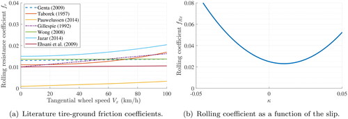
Another interesting approach was also presented Pauwelussen (2015), who described the rolling resistance force coefficient f_Rx as a function not only of the friction coefficient f_R, but also including the slip factor κ, the ratio between the load R_L and the effective R_e tire radii, and the normalized longitudinal slip stiffness $c_{\kappa },$ (also known as the parameter $P_{Kx1}$ from the Pacejka Magic Formula), as seen in Eq. (18)(18) $$f_{Rx}=\frac{R_L}{R_e}·c_{\kappa }·(1-\kappa )·\kappa +f_R-c_{\kappa }\kappa$$(18) . Figure 4(b) shows the f_Rx as a function of the slip κ, based on Pauwelussen (2015), considering a 195/65 R15 tire ($c_{\kappa }$ equal to 18.886), f_R of 0.025, and the ratio $R_L$/$R_e$ equal to 0.98. (18) $$f_{Rx}=\frac{R_L}{R_e}·c_{\kappa }·(1-\kappa )·\kappa +f_R-c_{\kappa }\kappa$$(18)

Applying Eq. (18)(18) $$f_{Rx}=\frac{R_L}{R_e}·c_{\kappa }·(1-\kappa )·\kappa +f_R-c_{\kappa }\kappa$$(18) to the analyzed case, the Eq. (17)(17) $$F_{\mathit{Res}}=f_r{F}_N$$(17) can be rewritten as seen in Eq. (19)(19) $$F_{\mathit{Res}}=f_{Rx}{F}_N$$(19) , where the rolling resistance force F_Res is a function of the f_Rx and the contact normal force F_N. Moreover, the torque T_Res caused by this force is obtained when multiplying Eq. (19)(19) $$F_{\mathit{Res}}=f_{Rx}{F}_N$$(19) by the roller radius r_r, as in Eq. (20)(20) $$T_{\mathit{Res}}=F_{\mathit{Res}}{r}_r$$(20) . (19) $$F_{\mathit{Res}}=f_{Rx}{F}_N$$(19) (20) $$T_{\mathit{Res}}=F_{\mathit{Res}}{r}_r$$(20)

3.3. System losses

In previous work, Eckert et al. (2017) had already analyzed the LabSIn’s dynamometer bench and raised the system losses $T_{{\mathrm{B}}_{\mathrm{L}}}$ and $T_{{\text{EM}}_{\mathrm{L}}},$ referent to the ECB and the EM as seen in Eqs. (21)(21) $$T_{{\mathrm{B}}_{\mathrm{L}}}=0.134V_{34}+3.67$$(21) and (22)(22) $$T_{{\text{EM}}_{\mathrm{L}}}=0.105V_{34}+3.67$$(22) , respectively. In this analysis, the bench was propelled by the vehicle and the read torques at the torque flanges were balanced at stabilized speeds V₃₄ (km/h), once the measurements were made at the 3 and 4 rollers axle. For both cases, the equations have a linear behavior according to the vehicle speed. (21) $$T_{{\mathrm{B}}_{\mathrm{L}}}=0.134V_{34}+3.67$$(21) (22) $$T_{{\text{EM}}_{\mathrm{L}}}=0.105V_{34}+3.67$$(22)

3.4. Components’ acting loads

Once the loads were described, the acting torques on each axle and its components are defined as seen in Eqs. (23)(23) $$T_{R12}=T_{\text{EM}}-T_{x12}-T_{\mathit{Res}12}$$(23) to (25)(25) $$T_{R34}=T_{x34}-T_{\mathit{Res}34}-T_{{\mathrm{B}}_{\mathrm{L}}}$$(25) , where $T_{R12}$ is the acting torque in rollers 1 and 2 axle, $T_{\text{EM}}$ is the torque provided by the EM, $T_{R34}$ is the torque in rollers 3 and 4 axle, $T_{{\mathrm{B}}_{\mathrm{L}}}$ is the torque loss caused by the breaking bench system, and n is the transmission ratio between tire r_e and roller r_r radii, obtained by Eq. (26)(26) $$n=\frac{r_e}{r_r}$$(26) . (23) $$T_{R12}=T_{\text{EM}}-T_{x12}-T_{\mathit{Res}12}$$(23) (24) $$T_w=(T_{x12}-T_{x34})·n$$(24) (25) $$T_{R34}=T_{x34}-T_{\mathit{Res}34}-T_{{\mathrm{B}}_{\mathrm{L}}}$$(25) (26) $$n=\frac{r_e}{r_r}$$(26)

From the second Newton’s Law, once the resultant torques and the component inertia are known, the accelerations of each axle are obtained as presented by Eqs. (27)(27) $$a_{R12}=\frac{T_{R12}}{I_{12}}$$(27) to (29)(29) $$a_{R34}=\frac{T_{R34}}{I_{34}}$$(29) , respectively the accelerations of the rollers 1 and 2 axle, the wheel axle, and the rollers 3 and 4 axle. (27) $$a_{R12}=\frac{T_{R12}}{I_{12}}$$(27) (28) $$a_w=\frac{T_w}{I_w}$$(28) (29) $$a_{R34}=\frac{T_{R34}}{I_{34}}$$(29)

For a total resistance analysis ($R_{\mathrm{T}}$), the Eq. (30)(30) $$R_{\mathrm{T}}=T_{x12}+T_{\mathit{Res}12}$$(30) was written as a function of the negative torques (resistances) acting on the 1 and 2 axle, therefore, the torque $T_{x12}$ and the rolling resistance torque $T_{\mathit{Res}12}.$ (30) $$R_{\mathrm{T}}=T_{x12}+T_{\mathit{Res}12}$$(30)

4. Simulation model

The model data flow is shown in Figure 5, where it is presented the wheel data in red (speed V_w, acceleration a_w, and acting torque T_w), the 1 and 2 rollers axle data in blue (speed V₁₂, acceleration a₁₂, and acting torque T₁₂), and the 3 and 4 rollers axle data in green (speed V₃₄, acceleration a₃₄, and acting torque T₃₄).

Figure 5. Flowchart modeling.

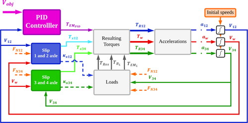
Firstly, initial speed values of 0.001 m/s were set to V₁₂, V₃₄ and V_w in order to initiate the process in all the blocks that require speed values. The Proportional-Integral-Derivative (PID) controller acts providing the EM desired torque aiming V₁₂ achieves the objective speed V_obj of the experiment. The initial speed values are also used to calculate the slips κ₁₂ and κ₃₄, as shown in Eq. (6)(6) $${\kappa }_x=\kappa +S_{Hx}$$(6) , and the slip torques in each rollers axle ($T_{x12}$ and $T_{x34}$), as in Eq. (16)(16) $$T_x=F_x{r}_r$$(16) .

Based on these variables, the main loads are obtained, such as the rolling resistance torque T_Res, as in Eq. (20)(20) $$T_{\mathit{Res}}=F_{\mathit{Res}}{r}_r$$(20) , and the systems losses, as proposed by Eckert et al. (2017) and shown in Eqs. (21)(21) $$T_{{\mathrm{B}}_{\mathrm{L}}}=0.134V_{34}+3.67$$(21) and (22)(22) $$T_{{\text{EM}}_{\mathrm{L}}}=0.105V_{34}+3.67$$(22) , depending on the speed V₃₄, once these losses data were acquired in the 3 and 4 rollers axle. With all the load information, the resulting torques are obtained by Eqs. (23)(23) $$T_{R12}=T_{\text{EM}}-T_{x12}-T_{\mathit{Res}12}$$(23) to (25)(25) $$T_{R34}=T_{x34}-T_{\mathit{Res}34}-T_{{\mathrm{B}}_{\mathrm{L}}}$$(25) . Then, with these torques and the inertia of the components, the accelerations are calculated as in Eqs. (27)(27) $$a_{R12}=\frac{T_{R12}}{I_{12}}$$(27) to (29)(29) $$a_{R34}=\frac{T_{R34}}{I_{34}}$$(29) and by integrating the accelerations the speed values are obtained for the next time step.

This logic was used in two modes: bench acceleration and coast-down. For the bench acceleration mode, the T_EM is equivalent to the torque set by the PID controller $T_{E{M}_{\mathit{PID}}}.$ For the coast-down analyses, the EM is turned off and becomes a source of losses and the T_EM assumes the value of $T_{E{M}_L},$ according to Eqs. (22)(22) $$T_{{\text{EM}}_{\mathrm{L}}}=0.105V_{34}+3.67$$(22) .

This logic was implemented in a Matlab/Simulink™ program, where ODE45 was the integrator. A PID controller adjusts the EM torque, where it was saturated at the maximum limit provided by EM after amplified by the planetary gears.

In this analysis, the parameters used are shown in Table 4 and the chosen vehicle was a FIAT™ Punto 2008 1.4 L. It is noteworthy the I₃₄ also considers the ECB inertia coupled in the 3 and 4 rollers axle. Moreover, due to the available tire model data, the simulated FM considered the tire 195/65 R15, as an approximation of the real tire 195/60 R15 (cold inflation pressure of 28 PSI) used at the experiment.

Table 4. Simulation parameters (Eckert et al. 2017, Eckert, Bertoti, et al. 2021).

Parameter	Value
Wheelbase L	2.51 m
Longitudinal distance between the CG and the rear axes b	1.50 m
Inertia of a tire-wheel assembly Iw	0.72 kgm^2
Inertia of the 1 and 2 roller bench axle I12	14.015 kgm^2
Inertia of the 3 and 4 roller bench axle I34	19.445 kgm^2
Vehicle mass m	1090 kg
Gravity acceleration g	9.80665 m/s^2
Unloaded tire (195/65 R15) radius rw	0.312 m
Roller radius rr	0.2 m
Friction coefficient fr	0.025
Tire radii ratio $R_L/R_e$	0.98

5. Results

After applying the simulation parameters in the logic presented in the previous section and in order to validate the model, the simulated results are compared with experimental data. In this article, two analysis are performed. The first is described in Subsection 5.1, where two coast-down approaches (starting at 60 km/h and at 100 km/h) are presented. Besides, a total resistance analysis is carried out in Subsection 5.2, showing the experimental loads and the ones achieved by the model. Moreover, Subsection 5.3 points out the details of the tire-roller contact, emphasizing the slip influence in the system speeds and torques.

5.1. Coast-down

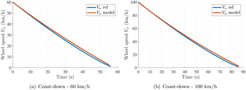
The coast-down procedure is ruled by the NBR10312 standard (NBR10312 2014) and it is currently applied to calibrate or adjust the dynamometers resistance with experimental data when the vehicle decelerates and it is set at a neutral position of the gearbox starting from a specific speed until its complete stop on a flat and rectilinear road (Preda, Covaciu, and Ciolan 2010). By standard, in this kind of experiment, the vehicle starts at 100 km/h, and the vehicle decelerates due to the movement resistances, mainly rolling resistance and aerodynamic drag. This procedure is often repeated on the dynamometer where the bench controller is adjusted following the standard procedure (NBR10312 2014) in order to reproduce the real test condition. Thus, as in the NBR10312 (2014), the coast-down analyses made in this section aim to calibrate the dynamometer model in order to make it as realistic as possible, supporting further analyses in future works.

In this work, a simplified and simulated coast-down procedure was performed and compared with the dynamometer coast-down experiment of a previous work (Eckert et al. 2017), where the vehicle was put at an initial speed, then, at neutral position of the gearbox, and the vehicle ran until the bench speed became null, without any power or breaking coming from the vehicle. This way, the experiments carried out by Eckert et al. (2017), and also the approach proposed in this article, did not consider the aerodynamic resistances. Firstly, the model simulates the procedure starting at 60 km/h. A comparison of the simulated V_wModel with the experimental data V_wRef is presented in Figure 6(a). Secondly, the coast-down experiment started from 100 km/h, according to the standard procedure (NBR10312 2014), and Figure 6(b) shows both experimental (V_wRef) and simulated results (V_wModel).

Figure 6. Coast-down comparisons.

In order to evaluate the model fit, the model errors were calculated as presented by Eq. (31)(31) $$\mathit{erro}{r}_{\text{CD}}(V_w)=|t_{\mathit{wRef}}-t_{\mathit{wModel}}|$$(31) , where t_wRef and t_wModel are the time-lapses to achieve each analyzed speed V_w by the reference experiment and the simulated model, respectively. (31) $$\mathit{erro}{r}_{\text{CD}}(V_w)=|t_{\mathit{wRef}}-t_{\mathit{wModel}}|$$(31)

For the coast-down starting at 60 km/h, the maximum error was 1.93 s (at 12.44 km/h) while the average value was 1.09 s. For 100 km/h initial speed, the maximum error was 2.88 s (at 12.27 km/h) while the average value was 1.32 s. The correlation coefficient R² was also calculated, resulting in 0.9998 for the 60 km/h case, and in 0.9999 for the 100 km/h case, indicating the simulated speed profiles are close enough to the experiment data and are representative results. Therefore, these results show the coast-down simulated represents the system experimental behavior for both cases of initial speeds.

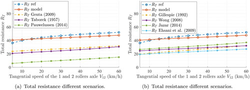
5.2. Total resistance

Aiming to evaluate the overall bench resistance with the vehicle, a total resistance analysis is performed. In previous work, Eckert et al. (2017) performed this experiment, which includes mechanical components friction losses, such as the ones in bearings, motors, powertrain, and reducers, and the losses due to the tire contact, as rolling resistance and slip of the tire. The aerodynamic drag was disregarded in this analysis.

The experiments measured the torque between the planetary (P) and the roller 1 (torque measurement point indicated in Figure 1), and they were repeated at different wheel tangential speeds in steps of 5 km/h, ranging from 5 km/h to 60 km/h. All acquisitions were taken after a stabilization speed period to eliminate the inertia effects, thereby, the measurement indicates the torque provided by the EM to overcome the resistances and keep the set experiment speed.

In the simulated model, the total torque resistance ($R_{\mathrm{T}\mathit{Model}}$) was evaluated during the acceleration mode as presented in Eq. (30)(30) $$R_{\mathrm{T}}=T_{x12}+T_{\mathit{Res}12}$$(30) , as the resistances at the measurement point at 1 and 2 rollers axle, for each stabilized speed, from 5 km/h to 60 km/h, as in the real test. Figure 7 shows the total resistance curves for the experiment ($R_{\mathrm{T}\mathit{Ref}}$), the model ($R_{\mathrm{T}\mathit{Model}}$) (slip-depended according to Eqs. (18)(18) $$f_{Rx}=\frac{R_L}{R_e}·c_{\kappa }·(1-\kappa )·\kappa +f_R-c_{\kappa }\kappa$$(18) and (19)(19) $$F_{\mathit{Res}}=f_{Rx}{F}_N$$(19) ), and the simulated total resistances considering well-established rolling resistances slip-independent equations from literature ($R_{\mathrm{T}}$ Genta and Morello (2009), $R_{\mathrm{T}}$ Taborek (1957), $R_{\mathrm{T}}$ Pauwelussen (2015), $R_{\mathrm{T}}$ Gillespie (1992), $R_{\mathrm{T}}$ Wong (2008), $R_{\mathrm{T}}$ Jazar (2014), $R_{\mathrm{T}}$ Ehsani, Gao, and Emadi (2009)), with the same previous friction coefficients presented in Figure 4 applied to Eq. (17)(17) $$F_{\mathit{Res}}=f_r{F}_N$$(17) . It is important to highlight all the rolling resistances equations, even the one on the final model, were originally developed for the single tire contact. The results presented in Figure 7 consider all these equations adapted to the double contact and applied as resistances in both rollers, as shown in Eqs. (23)(23) $$T_{R12}=T_{\text{EM}}-T_{x12}-T_{\mathit{Res}12}$$(23) and (25)(25) $$T_{R34}=T_{x34}-T_{\mathit{Res}34}-T_{{\mathrm{B}}_{\mathrm{L}}}$$(25) . The main difference is that the chosen equation for the model is a function of the tire slip.

Figure 7. Total resistances.

Similar to the coast-down analysis, for the total resistance the model error was figured applying Eq. (32)(32) $$e{r}_{R_T}=\frac{|(R_{\mathrm{T}\mathit{Ref}})-(R_{\mathrm{T}\mathit{Model}})|}{(R_{\mathrm{T}\mathit{Ref}})}$$(32) , where the mean error was 7.45% while the maximum error was 10.61% (at 5 km/h). The differences between the experimental and simulated resistances are due to the modeling approximations, such as the tire parameters, and to the approximately linear profile of the reference equation, if not at the hole domain, at least into the range limits reached by the simulation parameters, what happens for the rolling resistance and the slip equations. This feature implies the major error occurs at the limits of the speed range (5 km/h and 60 km/h), as seen in Figure 7. (32) $$e{r}_{R_T}=\frac{|(R_{\mathrm{T}\mathit{Ref}})-(R_{\mathrm{T}\mathit{Model}})|}{(R_{\mathrm{T}\mathit{Ref}})}$$(32)

The mean error was 7.45%, however, the literature presents much higher values at more simple models, as seen in Figure 7 and summarized in Table 5. Therefore, it is clear the well-established literature equations developed for tire-ground contacts cannot represent the tire-rollers contact, presenting mean errors in a range of 32.81% to 78.01%, while the maximum errors vary between 35.19% and 84.08%.

Table 5. Errors.

Errors	Model	Genta and Morello (2009)	Taborek (1957)	Pauwelussen (2015)	Gillespie (1992)	Wong (2008)	Jazar (2014)	Ehsani, Gao, and Emadi (2009)
% $e{r}_{R_{\mathrm{T}-\text{MEAN}}}$	7.45	40.71	46.16	78.01	44.84	39.38	32.81	50.46
% $e{r}_{R_{\mathrm{T}-\text{MAX}}}$	10.61	42.28	48.50	84.08	48.40	40.99	35.19	51.91

Even though Eq. (18)(18) $$f_{Rx}=\frac{R_L}{R_e}·c_{\kappa }·(1-\kappa )·\kappa +f_R-c_{\kappa }\kappa$$(18) was proposed by the literature for a tire-ground situation, it depends on the slips contact, which allows its adaptation for the tire-rollers case. This is possible only because the model considers the slip interactions, commonly disregarded in dynamometric bench studies. Therefore, for this analysis, the presented error variations are considered suitable, once there is no similar detailed research in this field.

5.3. Slip analysis

For the slip analysis, the acceleration mode (bench driven by the EM) was chosen with the maximum speed set at 60 km/h and simulation time of 35 s. Figure 8(a) shows the tangential speed values for each rotational axle, where the profile of the curves are very similar. It is noteworthy the speed values, which start from a stationary state, stabilize at the objective speed of 60 km/h near 21 s and, after this period, there are no significant variations. Besides, if Figure 8(a) is zoomed out, as presented in Figure 8(b), it is noticeable there is a gap between the curves, as a result of the slip occurring in the tire-rollers contact. As expected, the upper curve belongs to the motorized axle (1 and 2 rollers axle), followed by the wheel speed and then the 3 and 4 rollers axle speed. This effect happens due to the slip, which implies losses through the power transmission sequence.

Figure 8. Speed variation on the acceleration mode (driven by the bench EM) for a maximum speed of 60 km/h.

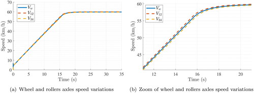
These behaviors are also seen in Figure 9(a) and (b), which presents the slip in each rollers axle contact and the torque changes during the simulations time, respectively. The slips are higher at the initial 15 s, where it happens a more severe acceleration, and, once the system tends to stabilize, they drop to values near zero, stabilizing around 21 s, as in the speed profiles. Moreover, as the major acting torque $T_{R12}$ is acting on the EM axle, as seen in Figure 9(b), the slip ${\kappa }_{x12}$ presents higher values then ${\kappa }_{x34},$ which is also noted in the lower value of $T_{R34},$ as expected. It is important to emphasize that, for the reached slip values, the simulation stays in the approximately linear domain of the FM curves (see Figure 3) and rolling resistance (see Figure 4(b)) chosen approaches.

Figure 9. Variations on the acceleration mode (driven by the bench EM) for a maximum speed of 60 km/h.

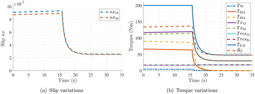
As mentioned in the previous graphs, the torque in Figure 9(b) follows the same stabilization time instants. The roller resistances curves $T_{\mathit{res}12}$ and $T_{\mathit{res}34}$ are overlaid, once they are a function of very close slips values, and almost at a constant level. The chosen rolling resistance approach elevates these values when compared to the literature equations developed to the single and plane tire-road contact, thereby, presenting a more compatible and realistic result. Furthermore, taking a closer look at torques in the 1 and 2 rollers axle, when the system stabilizes, the speed V₁₂ reaches the constant value while the resulting torque $T_{R12}$ goes near zero, once the driven torque $T_{\text{EM}}$ is balanced with the total resistance $R_{\mathrm{T}},$ causing the overlaid curves.

6. Conclusion

The article showed the relevance of vehicle testing and the applicability of chassis dynamometers as an experimental platform used by the automotive industry in development and homologation processes worldwide. On the other hand, it was also shown the literature gap regarding a representative model of a vehicle and a chassis dynamometer, considering the tire-roller contact.

This article presented the development of a dynamometer-vehicle model, merging the experimental and physical theories, including slip analysis, system losses, and rolling resistance, allowing a better representation of the vehicle-dynamometer real system. Thus, a model of the system resistance loads was presented and validated to represent the real laboratory test loads.

Experimental validation of the model showed average time variations of 1.11 s and 1.35 s, when compared with data from Eckert et al. (2017), for the coast-down analyses beginning at 60 km/h and 100 km/h, respectively. Besides, the correlation coefficients of 0.9998 (initial speed of 60 km/h) and 0.9999 (initial speed of 100 km/h) indicated very similar profiles between the simulated result and the experimental data. Further, for total resistant analysis, the mean error was 6.71%, an acceptable value when compared to experimental data and considering model approximations, since the literature equations, when applied in the model, presented mean errors of 31.94% to 77.61%. Therefore, it is clear the improvement brought by the development of the slip-dependent approach.

Thereby, the results show very similar behaviors between the experiment and the simulation, highlighting that the developed model is able to predict the longitudinal behavior. Moreover, the slip analysis showed an overview of the main parameter variation in the developed model, emphasizing the influence and importance of the slip in describing the vehicle-bench behavior.

Therefore, considering the applicability in real-case scenarios, the proposed model contributes to a better knowledge of vehicle behavior on a chassis dynamometer and its usage for vehicle analyses to attend to users’ and regulations’ requirements. With this approach, it is possible to pre-run experiments virtually (such as the ones mentioned in the next paragraph of future works), saving time and resources. Moreover, when applied to a system, the results will indicate the promising experiments could be successful with the physical bench infrastructure.

As future works, once the model is already validated, the next steps are to use the model as a pre-running and slip analysis tool for other experiments, such as acceleration and braking performances, following different standard driving cycles according to the studied vehicle and application field.

Disclosure statement

No potential competing interest was reported by the authors

Additional information

Funding

This work was supported by the University of Campinas (UNICAMP).

References

- 10521-2:2006(E). 2006, October. Road vehicles – Road load – Part 2: Reproduction on chassis dynamometer. International Organization for Standardization, Geneva, CH.
- 28981:2009(E). 2009, November. Methods for setting the running resistance on a chassis dynamometer. International Organization for Standardization, Geneva, CH.
- Aceituno, J. F., R. Chamorro, D. García-Vallejo, and J. L. Escalona. 2017. On the design of a scaled railroad vehicle for the validation of computational models. Mechanism and Machine Theory 115:60–76. doi:10.1016/j.mechmachtheory.2017.04.015.
- ADAMS. 2019. Tire Models. New Port Beach, CA: MSC.Software Corporation.
- Alcazar, M., J. Perez, J. Mata, J. Cabrera, and J. Castillo. 2020. Motorcycle final drive geometry optimization on uneven roads. Mechanism and Machine Theory 144:103647. doi:10.1016/j.mechmachtheory.2019.103647.
- Aldy, J., M. J. Kotchen, M. Evans, M. Fowlie, A. Levinson, and K. Palmer. 2021. Cobenefits and regulatory impact analysis: Theory and evidence from federal air quality regulations. Environmental and Energy Policy and the Economy 2 (1):117–56. doi:10.1086/711308.
- Barbosa, T. P., J. J. Eckert, L. C. A. Silva, L. A. R. da Silva, J. C. H. Gutiérrez, and F. G. Dedini. 2020. Gear shifting optimization applied to a flex-fuel vehicle under real driving conditions. Mechanics Based Design of Structures and Machines 1–18. doi:10.1080/15397734.2020.1769650.
- Beckers, C., I. Besselink, J. Frints, and H. Nijmeijer. 2019. Energy consumption prediction for electric city buses. In Proceedings of the 13th ITS European Congress, June 3–6, Brainport, Netherlands, Paper No. ITS-SP1813, 1–12.
- Bertoti, E., R. Yamashita, J. Eckert, F. Santiciolli, F. Dedini, and L. Silva. 2019. Application of pattern recognition for the mitigation of systematic errors in an optical incremental encoder. In Proceedings of the 10th international conference on rotor dynamics (IFToMM), Vol. 4, 65–78. New York: Springer.
- Besselink, I., A. Schmeitz, and H. Pacejka. 2010. An improved Magic Formula/Swift Tyre model that can handle inflation pressure changes. Vehicle System Dynamics 48 (sup1):337–52. doi:10.1080/00423111003748088.
- Bielaczyc, P., J. Woodburn, and A. Szczotka. 2016. Exhaust emissions of gaseous and solid pollutants measured over the NEDC, FTP-75 and WLTC chassis dynamometer driving cycles. In SAE 2016 World Congress and Exhibition. SAE International.
- Chen, J., C. Liu, X.-Z. Zhang, Y.-B. Zhang, and J.-Z. Li. 2021. An approach for indoor prediction of the pass-by noise of a vehicle based on the time-domain equivalent source method. Mechanical Systems and Signal Processing 146:107037. doi:10.1016/j.ymssp.2020.107037.
- Chen, T., X. Xu, L. Chen, H. Jiang, Y. Cai, and Y. Li. 2018. Estimation of longitudinal force, lateral vehicle speed and yaw rate for four-wheel independent driven electric vehicles. Mechanical Systems and Signal Processing 101:377–88. doi:10.1016/j.ymssp.2017.08.041.
- Delkhosh, M., M. S. Foumani, and M. Boroushaki. 2014. Geometrical optimization of parallel infinitely variable transmission to decrease vehicle fuel consumption. Mechanics Based Design of Structures and Machines 42 (4):483–501. doi:10.1080/15397734.2014.888314.
- Dong, X., B. Zhang, B. Wang, and Z. Wang. 2020. Urban households’ purchase intentions for pure electric vehicles under subsidy contexts in china: Do cost factors matter? Transportation Research Part A: Policy and Practice 135:183–97. doi:10.1016/j.tra.2020.03.012.
- Eckert, J. J., E. Bertoti, E. dos Santos Costa, F. M. Santiciolli, R. Y. Yamashita, L. C. Silva, and F. G. Dedini. 2017. Experimental evaluation of rotational inertia and tire rolling resistance for a twin roller chassis dynamometer. Technical report, SAE Technical Paper.
- Eckert, J. J., E. Bertoti, L. C. A. Silva, and F. G. Dedini. 2021. Experimental validation for the employment of shifting strategies optimized via i-awga in a gear shift indicator system for manual transmission vehicles. Mechanics Based Design of Structures and Machines 1–22. doi:10.1080/15397734.2021.1911664.
- Eckert, J. J., Í. P. Teodoro, L. H. Teixeira, T. S. Martins, P. R. G. Kurka, and A. A. Santos. 2021. A fast simulation approach to assess draft gear loads for heavy haul trains during braking. Mechanics Based Design of Structures and Machines 1–20. doi:10.1080/15397734.2021.1875233.
- Eckert, J. J., S. F. da Silva, F. M. Santiciolli, Á. Chagas de Carvalho, and F. G. Dedini. 2022. Multi-speed gearbox design and shifting control optimization to minimize fuel consumption, exhaust emissions and drivetrain mechanical losses. Mechanism and Machine Theory 169:104644. doi:10.1016/j.mechmachtheory.2021.104644.
- Eckert, J. J., F. M. Santiciolli, L. C. Silva, and F. G. Dedini. 2021. Vehicle drivetrain design multi-objective optimization. Mechanism and Machine Theory 156:104123. doi:10.1016/j.mechmachtheory.2020.104123.
- Eckert, J. J., L. C. de Alkmin e Silva, E. dos Santos Costa, F. M. Santiciolli, F. C. Corrêa, and F. G. Dedini. 2019. Optimization of electric propulsion system for a hybridized vehicle. Mechanics Based Design of Structures and Machines 47 (2):175–200. doi:10.1080/15397734.2018.1520129.
- Ehsani, M., Y. Gao, and A. Emadi. 2009. Modern electric, hybrid electric, and fuel cell vehicles: Fundamentals, theory, and design. Boca Raton, FL: CRC Press.
- Ejsmont, J., and W. Owczarzak. 2019. Engineering method of tire rolling resistance evaluation. Measurement 145:144–9. doi:10.1016/j.measurement.2019.05.071.
- Euler-Rolle, N., C. H. Mayr, I. Škrjanc, S. Jakubek, and G. Karer. 2020. Automated vehicle driveaway with a manual dry clutch on chassis dynamometers: Efficient identification and decoupling control. ISA Transactions 98:237–50. doi:10.1016/j.isatra.2019.08.021.
- Fajri, P., M. Ferdowsi, N. Lotfi, and R. Landers. 2016. Development of an educational small-scale hybrid electric vehicle (HEV) setup. IEEE Intelligent Transportation Systems Magazine 8 (2):8–21. doi:10.1109/MITS.2015.2505739.
- Gao, X., Y. Xiong, W. Liu, and Y. Zhuang. 2021. Modeling and experimental study of tire deformation characteristics under high-speed rolling condition. Polymer Testing 99:107052. doi:10.1016/j.polymertesting.2021.107052.
- Genta, G., and L. Morello. 2009. The automotive chassis, Volume 1. New York: Springer.
- Ghadge, R. R., and S. Prakash. 2021. Investigation and prediction of hybrid composite leaf spring using deep neural network based rat swarm optimization. Mechanics Based Design of Structures and Machines 1–30. doi:10.1080/15397734.2021.1972309.
- Gillespie, T. D. 1992. Fundamentals of vehicle dynamics. Warrendale, PA: Society of Automotive Engineers - SAE.
- Habermehl, C., G. Jacobs, and S. Neumann. 2020. A modeling method for gear transmission efficiency in transient operating conditions. Mechanism and Machine Theory 153:103996. doi:10.1016/j.mechmachtheory.2020.103996.
- Jazar, R. N. 2014. Vehicle dynamics: Theory and application. Berlin: Springer Science & Business Media.
- Jouanne, A. V., J. Adegbohun, R. Collin, M. Stephens, B. Thayil, C. Li, E. Agamloh, and A. Yokochi. 2020. Electric vehicle (ev) chassis dynamometer testing. In 2020 IEEE Energy Conversion Congress and Exposition (ECCE), 897–904.
- Kim, Y.-D., J.-E. Jeong, J.-S. Park, I.-H. Yang, T.-S. Park, P. B. Muhamad, D.-H. Choi, and J.-E. Oh. 2013. Optimization of the lower arm of a vehicle suspension system for road noise reduction by sensitivity analysis. Mechanism and Machine Theory 69:278–302. doi:10.1016/j.mechmachtheory.2013.06.010.
- Lairenlakpam, R., P. Kumar, and G. D. Thakre. 2019. Experimental investigation of electric vehicle performance and energy consumption on chassis dynamometer using drive cycle analysis. SAE International Journal of Sustainable Transportation, Energy, Environment, & Policy 1:23–38.
- Lohse-Busch, H., K. Stutenberg, M. Duoba, X. Liu, A. Elgowainy, M. Wang, T. Wallner, B. Richard, and M. Christenson. 2020. Automotive fuel cell stack and system efficiency and fuel consumption based on vehicle testing on a chassis dynamometer at minus 18 °c to positive 35 °c temperatures. International Journal of Hydrogen Energy 45 (1):861–72.
- Martyr, A., and M. Plint. 2012. Chassis or rolling-road dynamometers. Chapter 17. In Engine testing, eds. A. Martyr and M. Plint, 4th ed., 451–82. Oxford: Butterworth-Heinemann.
- Matthews, C. 2007. Identification and robust control of automotive dynamometers. PhD thesis, University of Liverpool.
- Mayyas, A., S. Kumar, P. Pisu, J. Rios, and P. Jethani. 2017. Model-based design validation for advanced energy management strategies for electrified hybrid power trains using innovative vehicle hardware in the loop (VHIL) approach. Applied Energy 204:287–302. doi:10.1016/j.apenergy.2017.07.028.
- Miranda, M. H., F. L. Silva, M. A. Lourenço, J. J. Eckert, and L. C. Silva. 2022. Electric vehicle powertrain and fuzzy controller optimization using a planar dynamics simulation based on a real-world driving cycle. Energy 238:121979. doi:10.1016/j.energy.2021.121979.
- NBR10312. 2014. Light duty road vehicles—Road load measurement and dynamometer simulation using coast down techniques. ABNT.
- O’Neill, A., J. Prins, J. F. Watts, and P. Gruber. 2021. Enhancing brush Tyre model accuracy through friction measurements. Vehicle System Dynamics 1–23. doi:10.1080/00423114.2021.1893766.
- Pałasz, B., K. Waluś, and u Warguła. 2019, 01. The determination of the rolling resistance coefficient of a passenger vehicle with the use of selected road tests methods. MATEC Web of Conferences 254:04006. doi:10.1051/matecconf/201925404006.
- Pacejka, H. B. 2012. Tire and vehicle dynamics, volume 3. Oxford: Butterworth-Heinemann.
- Pan, Y., W. Dai, Y. Xiong, S. Xiang, and A. Mikkola. 2020. Tree-topology-oriented modeling for the real-time simulation of sedan vehicle dynamics using independent coordinates and the rod-removal technique. Mechanism and Machine Theory 143:103626. doi:10.1016/j.mechmachtheory.2019.103626.
- Pauwelussen, J. P. 2015. Essentials of vehicle dynamics. Amsterdam, Netherlands: Elsevier.
- Pexa, M., D. Mader, J. Čedík, B. Peterka, M. Müller, P. Valášek, and S. Hloch. 2020. Experimental verification of small diameter rollers utilization in construction of roller test stand in evaluation of energy loss due to rolling resistance. Measurement 152:107287. doi:10.1016/j.measurement.2019.107287.
- Preda, I., D. Covaciu, and G. Ciolan. 2010. Coast down test – Theoretical and experimental approach. Paper presented at CONAT 2010 - International Automotive Congress, Brasov, Romania, paper 4030.
- Roso, V. R., N. D. S. A. Santos, R. M. Valle, C. E. C. Alvarez, J. Monsalve-Serrano, and A. García. 2019. Evaluation of a stratified prechamber ignition concept for vehicular applications in real world and standardized driving cycles. Applied Energy 254:113691. doi:10.1016/j.apenergy.2019.113691.
- Salehi, M., J. W. M. Noordermeer, L. A. E. M. Reuvekamp, and A. Blume. 2021. Understanding test modalities of tire grip and laboratory-road correlations with modeling. Tribology Letters 69 (3):116. doi:10.1007/s11249-021-01490-2.
- Salehi, M., J. W. M. Noordermeer, L. A. E. M. Reuvekamp, T. Tolpekina, and A. Blume. 2020. A new horizon for evaluating tire grip within a laboratory environment. Tribology Letters 68 (1):37. doi:10.1007/s11249-020-1273-5.
- Shangguan, W.-B., X.-A. Liu, Z.-P. Lv, and S. Rakheja. 2016. Design method of automotive powertrain mounting system based on vibration and noise limitations of vehicle level. Mechanical Systems and Signal Processing 76–77:677–95. doi:10.1016/j.ymssp.2016.01.009.
- Silva, L., F. Dedini, F. Corrêa, J. Eckert, and M. Becker. 2016. Measurement of wheelchair contact force with a low cost bench test. Medical Engineering & Physics 38 (2):163–70. doi:10.1016/j.medengphy.2015.11.014.
- Silva, L. C. A., J. J. Eckert, M. A. M. Lourenço, F. L. Silva, F. C. Corrêa, and F. G. Dedini. 2021. Electric vehicle battery-ultracapacitor hybrid energy storage system and drivetrain optimization for a real-world urban driving scenario. Journal of the Brazilian Society of Mechanical Sciences and Engineering 43 (5):259. doi:10.1007/s40430-021-02975-w.
- Silva, S. F., J. J. Eckert, F. L. Silva, L. C. Silva, and F. G. Dedini. 2021. Multi-objective optimization design and control of plug-in hybrid electric vehicle powertrain for minimization of energy consumption, exhaust emissions and battery degradation. Energy Conversion and Management 234:113909. doi:10.1016/j.enconman.2021.113909.
- Soica, A., A. Budala, V. Monescu, S. Sommer, and W. Owczarzak. 2020. Method of estimating the rolling resistance coefficient of vehicle Tyre using the roller dynamometer. Proceedings of the Institution of Mechanical Engineers, Part D: Journal of Automobile Engineering 234 (13):3194–204. doi:10.1177/0954407020919546.
- Song, K., F. Li, X. Hu, L. He, W. Niu, S. Lu, and T. Zhang. 2018. Multi-mode energy management strategy for fuel cell electric vehicles based on driving pattern identification using learning vector quantization neural network algorithm. Journal of Power Sources 389:230–9. doi:10.1016/j.jpowsour.2018.04.024.
- Taborek, J. J. 1957. Mechanics of vehicles. Cleveland, OH: Penton.
- Wager, G., M. McHenry, J. Whale, and T. Braunl. 2014. Testing energy efficiency and driving range of electric vehicles in relation to gear selection. Renewable Energy 62:303–12. doi:10.1016/j.renene.2013.07.029.
- Wong, J. Y. 2008. Theory of ground vehicles. New York: John Wiley & Sons.