Design, rapid manufacturing and modeling of a reduced-scale forwarder crane with closed kinematic chain

Abstract

Forestry cranes are of paramount importance in forestry operations, so considerable efforts have been carried out to improve their performance in recent years. However, all these efforts have focused on automation technology, leaving aside other alternatives for improvement. Among these alternatives is model-based design, which has the potential to be game-changing for the forest industry. Because research on model-based design is almost non-existent for forestry cranes, there are many gaps that should be filled before presenting improved designs of forestry cranes. The purpose of this article is to fill two of those gaps: (1) the high cost-benefit ratio and safety concerns when testing new designs, components or algorithms in industrial-scale forestry cranes and (2) the dynamic modeling of forestry cranes as mechanical systems with closed kinematic chain. Under these premises, this article first presents a reduced-scale platform resembling a forwarder crane with closed-kinematic chain, where the components of the mechanical structure are manufactured with 3D printing technology, and second, the modeling and experimental validation of the reduced-scale forwarder, where the closed kinematic chain is considered as a system of multiple constrained open kinematic chains. For the experimental validation, a comparison between both experimental and simulation results is presented. Results presented in this article broaden the options to design and test new concepts and/or technology to improve forestry cranes performance.

Keywords:

• Forestry cranes
• dynamic modeling
• 3D printing
• simulations
• experimental validation

1. Introduction

In Nordic countries, forestry cranes are the primary tool for harvesting and collecting logs in logging operations when considering the cut-to-length (CTL) method (Häggström and Lindroos 2016; Nordfjell et al. 2019; Ortiz Morales et al. 2014). This method typically considers a scheme of work with two human-operated forestry cranes: a harvester crane for felling, delimbing and bucking trees (Fig. 1a), and a forwarder crane for collecting and transporting logs to the yard for unloading (Fig. 1b).

Figure 1. Commercial harverster and forwarder cranes from VIMEK.

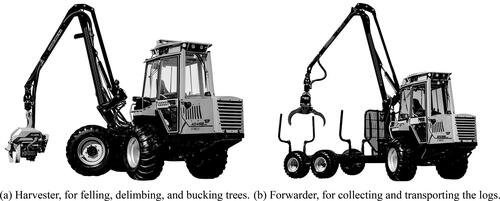
At present, the performance and productivity of forestry cranes rely heavily on human operators, and therefore, their experience to maintain a good work pace by using as few resources as possible. Nevertheless, due to the characteristics of these machines (size, weight, and difficulty to control), only the most experienced operators can achieve high levels of productivity. This situation is indeed a huge challenge for forestry crane manufacturers since highly skilled operators are lacking. To put this into perspective, it is important to mention that in Nordic countries, forestry crane operators must approve an exam where practical skills, technical knowledge, and the ability to work in the forest are evaluated. The evaluation and learning process for a person to get a job license takes approximately one year, however, it takes many years to be a highly skilled operator. Besides, the number of operator candidates has reduced over time, since it is a lonely job with exposure to high vibration levels that affect the human body (Häggström and Lindroos 2016; Ortiz Morales et al., 2015, Ortiz Morales et al. 2014). All these drawbacks have changed the vision of forestry crane manufacturers, and have led them to consider different technological solutions to improve their products and human operators’ performance (Morales et al.., 2015, Ortiz Morales et al. 2014).

In the last decade, most technological solutions to improve the performance of forestry cranes have focused on controlling the cranes by using smart automation software (Kalmari, Backman, and Visala 2017; Mattila et al. 2017; Ortiz Morales et al. 2014). These efforts have produced results that can be seen in existing products on the market, such as Cartesian controls (boom tip control), where human operators do not need to control each cylinder individually, but directly control the movement of the end-effector (boom tip) (Kalmari, Backman, and Visala 2017; Manner, Mörk, and Englund 2019). It is undeniable that there have been improvements and advances in the automation area of forestry cranes that facilitate the work of human operators, however, many researchers have shown that automation in forestry is still at the early stage, as there are many challenges that still have to be solved and understood, such as the highly nonlinear dynamic behavior of articulated hydraulic systems and the unpredictable performance of human operators using forestry cranes (La Hera and Ortiz Morales 2019; Mattila et al. 2017; Vihonen, Mattila, and Visa 2017).

The current situation regarding automation and control of forestry cranes makes it important to explore other improvement alternatives for forestry cranes. One of the areas that has been almost ignored by the forest industry over the years is model-based design. This design approach involves obtaining multidomain physics models describing the dynamic behavior of a mechanical system, which can be easily scaled to different types or sizes of machines. Due to its versatility and efficiency, this approach has been widely used to design, control and improve different types of systems, for instance, human-robot collaboration systems, robot gripper mechanisms, parallel robots, and vehicles (Eckert et al. 2018; Gaz, Magrini, and De Luca 2018; Hassan and Abomoharam 2017; Vallés et al. 2018). Forestry cranes design has not changed in decades, what has changed is the size, they have become bigger and heavier, implying that fuel consumption and ground damage have also increased (Häggström and Lindroos 2016; Nordfjell et al. 2019). Model-based design can change this situation and bring enormous benefits in terms of performance and productivity to the forest industry, however, some theoretical and technological aspects must be tackled before proposing improved designs of forestry cranes. The success of this design approach depends mainly on the elements/components in the model and how they are taken into account, so it is important to get a model considering as many conditions and elements as possible. The nonlinear dynamic model of an industrial forestry crane as an open kinematic chain was presented in (La Hera and Ortiz Morales 2014), nevertheless, forestry cranes often use closed kinematic chains, so it is necessary to present a model where all conditions, constraints and the highly-coupled dynamic response of this type of kinematic chains are considered (Koivumäki and Mattila 2015). By considering the closed kinematic chain, a more accurate dynamic model will be obtained. In addition, elements and conditions that can be taken into account in the design process will also be increased.

When comparing model-based design on other similar heavy-duty machinery, for instance hydraulic excavators, the situation is not much different. In general, most design and modeling efforts consider hydraulic excavators as mechanical systems with open kinematic chains (Li et al. 2017; Mitrev and Marinković 2019; Salinić, Bosković, and Nikolić 2014; Xu, Ding, and Feng 2019). In (Mitrev, Janosević, and Marinković 2017), authors considered a hydraulic excavator as a multibody system with both, open and closed kinematic chains. The modeling methodology used by the authors leads to a DAE system of index 3, which implies higher complexity and computational effort. This is because the solution of DAE systems involves the simultaneous solution of an ODE system and algebraic constraints (Arnold 2017; Mendoza-Trejo and Cruz-Villar 2016). By using the modeling methodology presented in (Park, Choi, and Ploen 1999), an ODE system is directly obtained, which can be solved by classical integration methods, such as the fourth-order Runge-Kutta method.

Moreover, one of the main problems when considering model-based design is the test phases. Testing new designs at early stages by manufacturing industrial-size prototypes has a high cost-benefit ratio that most companies cannot afford. One possible solution to high-cost and safety concerns is reduced-scale prototypes, which have been widely used in different systems. Some examples include reduced-scale vehicles for testing control strategies (Brennan and Alleyne 2001), reduced-scale Francis turbines to identify the eigenfrequencies and eigenmodes of a hydraulic system (Favrel et al. 2019), and reduced-scale platforms to detect and diagnose system elevator failures (Esteban et al. 2017). Conditions regarding high-cost benefit ratio are not different for forestry cranes. Forces exerted by the hydraulic actuators in industrial-size cranes are extremely high, so failures during test phases may cause significant material and human damages. This situation shows the need for a low-cost and safe platform to continue developing advances in forestry cranes.

1.1. Main Contribution

Considering the problems described in the previous paragraphs, this article aims at the following two points:

1. Present a reduced-scale platform for testing new designs, components and/or automation software in forestry cranes. Rapid manufacturing via 3D printing technology has had significant progress and has been used frequently for prototyping (Bin Ishak, Fleming, and Larochelle 2019; Bin Ishak and Larochelle 2019; Mick et al. 2019), so the mechanical structure of our prototype was manufactured by using metal 3D printing technology. Additional components, such as electronic devices for signal acquisition and control, as well as different actuators are shown in detail in Section 2.

2. Reduce the knowledge gap regarding the model-based design of forestry cranes by presenting both, the dynamic model and the experimental validation of a reduced-scale forwarder crane with closed kinematic chain. For modeling purposes, we consider the closed kinematic chain of the forestry crane as a system of multiple constrained open kinematic chains (Park, Choi, and Ploen 1999; Siciliano et al. 2010). It is well known that mechanical systems with closed kinematic chains generally have higher precision and dynamic performance, implying that greater benefits can be expected when taking into account these kinematic structures in the design process. The dynamic model presented in this article represents the first step toward improving forestry cranes when considering model-based design. This model will allow to modify all the crane’s inertial parameters in an easy, quick and efficient way. At the same time, the possibility of combining the dynamic model with other improvement options (such as mathematical optimization) is enabled.

Explanatory notes

For this paper, we worked on the following bases:

• We took as a base design for the modeling process the forwarder crane shown in Fig. 1b. This is a small-size forwarder crane that is mainly used for small-diameter trees and does not have the characteristic telescopic link. This crane was chosen as the base model as its closed kinematic chain is more complex than the closed kinematic chains found in cranes with telescopic links. However, the modeling procedure presented in this article can be applied to other types of forestry cranes.

• Due to copyright restrictions, the reduced–scale forestry crane used in this article does not represent an exact replica of any specific commercial crane. However, the design used for this article keeps the kinematic structure as similar as possible to commercially available forwarder cranes.

• Since we are only interested in presenting the dynamic model of the closed kinematic chain, the gripper and hydraulic elements are not taken into account. Interested readers on how to model and consider the hydraulic system can find detailed information in (La Hera and Ortiz Morales 2014).

2. Material and methods

2.1. Overview of the Reduced-Scale forestry crane

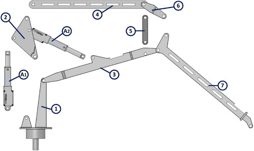
The reduced-scale prototype’s main components and design are shown in Fig. 2, while its physical properties and characteristics are shown in the following sections.

Figure 2. Main components of the reduced-scale experimental platform.

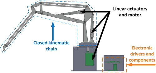
2.1.1. Mechanical structure – Closed kinematic chain

For the mechanical structure design, we took as main references the dimensions and workspace of the forwarder crane shown in Fig. 1(b). Dimensions of the reduced-scale prototype are proportional to those of an industrial crane and were constrained by the maximum dimensions that can be manufactured by 3 D printers and off-the-shelf linear actuators.

All elements composing the closed kinematic chain were separately designed in CATIA V5® and subsequently assembled for the final design.

2.1.2. Linear actuators and motor

The forwarder crane of Fig. 2 has three degrees of freedom (3-dof), with two linear actuators and one motor with a gearbox. For the linear actuators, L-12-P series micro linear actuators produced by Actuonix^® were selected. Both linear actuators have a stroke length of 30 mm, a gearbox with a transmission ratio of 210:1, and an internal analog potentiometer to provide position feedback. The voltage on the potentiometer central terminal will vary linearly between two reference voltages in proportion to the position of the actuator stroke. For the motor with gearbox, we selected the 37 D Polulu^®. This motor has a gearbox transmission ratio of 131:1, while the position feedback is provided by an integrated encoder with 64 cycles per revolution, implying that it is possible to measure as low as 0.042 degrees.

2.1.3. Electronic drivers and components

This work considers the experimental validation of a reduced-scale forwarder crane, so closed-loop experiments are needed. To this end, we use electronic drivers to send control signals to the actuators, as well as an electronic board to acquire, process and control data. We selected the real-time processing unit STM32F42DISCOVERY. This board contains a 32-bit Arm Cortex^® -M4, analog inputs/outputs, digital inputs/outputs, and a direct interface with MATLAB^® Simulink^®.

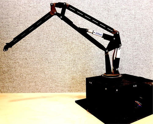
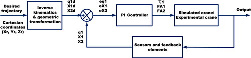
For the experimental validation, we consider a comparison between real and simulated values of forces and torques. Since neither the linear actuators nor the electric motor has force/torque sensors, it is necessary to compute those values from their actuation current. To measure the current used by these devices, we designed a circuit based on low impedance resistors. This circuit is connected to a commercial L298N motor driver, allowing to carry out two actions simultaneously: measuring the current used by the actuators/motor and enabling the actuation device’s movement in both directions. Controllers and electronic components selection was made in accordance with the operating specifications provided by the manufacturers of the linear actuators and motor. The block diagram of Fig. 3 shows how the electronic components, the board and the drivers work together to control the actuators’ movements, while Fig. 4 shows a picture of the actual experimental prototype.

Figure 3. Block diagram for the electronic drivers and the electronic components.

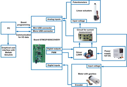
Figure 4. Reduced-scale forwarder crane.

2.2. Dynamic Model of a forwarder crane as a system with closed kinematic chain

The procedure for deriving mathematical models representing systems dynamics with closed kinematic chain (CKC) differs from standard procedures for systems with open kinematic chain (OKC). In this article, we consider the procedure described in (Park, Choi, and Ploen 1999) and (Siciliano et al. 2010), which aims to derive the system dynamic model as a function of the active joint variables ${\mathbf{q}}_{\mathbf{A}}\in {\mathbf{R}}^{\mathrm{n}},$ where $\mathrm{n}$ represents the number of active joints and corresponds to the system degrees of freedom.

The procedure starts by dividing the CKC into multiple OKCs. This division allows to derive dynamic models of the OKCs in terms of the set of passive and active joints ${\mathbf{q}}_{\mathbf{PA}}\in {\mathbf{R}}^{\mathrm{m}}:\mathrm{n}<\mathrm{m}.$ Finally, after deriving the dynamic models of the OKCs, the system dynamics in terms of ${\mathbf{q}}_{\mathbf{PA}}$ is transformed into terms of ${\mathbf{q}}_{\mathbf{A}}.$ For interested readers, this procedure can be seen in detail in (Park, Choi, and Ploen 1999) and (Siciliano et al. 2010).

2.2.1. Division of the closed kinematic chain

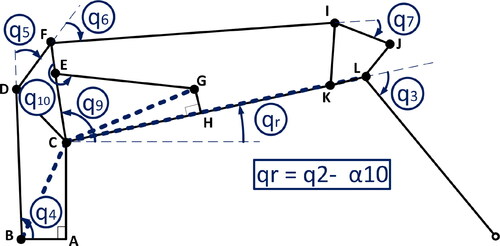
The first step to derive the dynamic model of the forwarder crane in Fig. 4 is to divide the CKC into multiple OKCs. When dividing the CKC, it is important to note that each element (link) can only be part of one OKC, that is, repetitions of elements in the open chains are not allowed.

Referring to Fig. 5, we consider five open kinematic chains. Chain A is composed of links 1, 3 and 7. Chain ${\mathrm{B}}_1$ is composed of linear actuator ${\mathrm{A}}_1.$ Chain ${\mathrm{B}}_2$ is composed of links 4 and 6, while chain C is composed of link 2 and linear actuator A₂. Finally, chain D is composed of link 5.

Figure 5. Forwarder crane as a system of multiple open kinematic chains.

2.2.2. Kinematic modelling of the open kinematic chains

Forward kinematics allows determining the position and orientation of different elements in a system from specified values for joint variables. In our case, we are interested in obtaining the position and orientation of all elements (links) composing the five OKCs. For this purpose, we use the well-known Denavit-Hartenberg (DH) convention (Spong, Hutchinson, and Vidyasagar 2006), where the position and orientation of the links are represented by the homogeneous transformation matrix, $${\mathrm{A}}_{\mathrm{i}}={\text{Rot}}_{\mathrm{Z},{\theta }_{\mathrm{i}}}{\text{Trans}}_{\mathrm{Z},{\mathrm{d}}_{\mathrm{i}}}{\text{Trans}}_{\mathrm{X},{\mathrm{a}}_{\mathrm{i}}}{\text{Rot}}_{\mathrm{X},{\alpha }_{\mathrm{i}}}.$$

Although all chains are analyzed separately, they must have the same base reference frame ${\mathrm{X}}_0,{\mathrm{Y}}_0,{\mathrm{Z}}_0.$ In addition, if auxiliary reference frames are needed, and these frames have been previously established in other chains, the new frames must match the previous frames. The detailed procedure to get the forward kinematics of the OKCs can be seen in A.

2.2.3. Dynamic modeling of the closed kinematic chain

The first step to obtaining the dynamic model of the CKC is to use standard procedures of robot modeling to obtain the dynamics of the OKCs, for instance, the Euler-Lagrange formulation described in (Spong, Hutchinson, and Vidyasagar 2006). Considering this formulation, dynamics of the OKCs can be represented by a system of second order differential equations as follows, (1) $$\mathbf{D}(\mathbf{q})\stackrel{\mathbf{"}}{\mathbf{q}}\mathit{+}\mathbf{C}(\mathbf{q},\stackrel{\mathbf{̇}}{\mathbf{q}})\stackrel{\mathbf{̇}}{\mathbf{q}}\mathit{+}\mathbf{G}(\mathbf{q})\mathit{=\tau },$$(1) where q $\in {\mathbf{R}}^{\eta \times 1}$ represents the vector of generalized coordinates, $\mathbf{D}(\mathbf{q})\in {\mathbf{R}}^{\eta \times \eta }$ represents the mass and inertia matrix, $\mathbf{C}(\mathbf{q},\stackrel{\mathbf{̇}}{\mathbf{q}})\in {\mathbf{R}}^{\eta \times \eta }$ represents the Coriolis matrix, $\mathbf{G}(\mathbf{q})\in {\mathbf{R}}^{\eta \times 1}$ represents the gravity vector, $\mathit{\tau }\in {\mathbf{R}}^{\eta \times 1}$ represents the forces and torques vector and η represents the number of generalized coordinates.

After deriving the dynamic model of each OKC, it is necessary to get an equation where all dynamic models of each OKC are simultaneously considered. This equation represents the dynamic model without constraints and is stated as function of the set of passive and active joints ${\mathbf{q}}_{\mathbf{PA}}.$ The detailed procedure and nomenclature used to get this representation can be seen in B.

The general equation representing the CKC’s dynamic model without constraints as a function of ${\mathbf{q}}_{\mathbf{PA}}$ is presented in Eq. (2)(2) $$\begin{array}{c}{\mathbf{D}}_{\mathbf{PA}}({\mathbf{q}}_{\mathbf{PA}})\stackrel{..}{{\mathbf{q}}_{\mathbf{PA}}}\mathit{+}{\mathbf{C}}_{\mathbf{PA}}({\mathbf{q}}_{\mathbf{PA}},\stackrel{.}{{\mathbf{q}}_{\mathbf{PA}}})\stackrel{.}{{\mathbf{q}}_{\mathbf{PA}}}\hfill \\ \mathit{+}{\mathbf{G}}_{\mathbf{PA}}({\mathbf{q}}_{\mathbf{PA}})\mathit{=}{\mathit{\tau }}_{\mathbf{PA}},\hfill \\ {\mathbf{q}}_{\mathbf{PA}}=\begin{array}{c}\left(\begin{array}{c}{q}_1\\ q_2\\ q_3\\ q_4\\ X1\\ q_6\\ q_7\\ q_9\\ q_{10}\\ X2\\ q_{11}\end{array}\right)\hfill \end{array};{\mathit{\tau }}_{\mathbf{PA}}=\begin{array}{c}\left(\begin{array}{c}{\tau }_1\\ {\tau }_2\\ {\tau }_3\\ {\tau }_4\\ F_{A1}\\ {\tau }_6\\ {\tau }_7\\ {\tau }_9\\ {\tau }_{10}\\ F_{A2}\\ {\tau }_{11}\end{array}\right)\hfill \end{array}.\hfill \end{array}$$(2) , where ${\mathbf{D}}_{\mathbf{PA}}({\mathbf{q}}_{\mathbf{PA}})\in {\mathbf{R}}^{11\times 11}$ is the inertia matrix, ${\mathbf{C}}_{\mathbf{PA}}({\mathbf{q}}_{\mathbf{PA}},\stackrel{.}{{\mathbf{q}}_{\mathbf{PA}}})\in {\mathbf{R}}^{11\times 11}$ represents the Coriolis matrix and ${\mathbf{G}}_{\mathbf{PA}}({\mathbf{q}}_{\mathbf{PA}})\in {\mathbf{R}}^{11\times 1}$ represents the gravity vector. (2) $$\begin{array}{c}{\mathbf{D}}_{\mathbf{PA}}({\mathbf{q}}_{\mathbf{PA}})\stackrel{..}{{\mathbf{q}}_{\mathbf{PA}}}\mathit{+}{\mathbf{C}}_{\mathbf{PA}}({\mathbf{q}}_{\mathbf{PA}},\stackrel{.}{{\mathbf{q}}_{\mathbf{PA}}})\stackrel{.}{{\mathbf{q}}_{\mathbf{PA}}}\hfill \\ \mathit{+}{\mathbf{G}}_{\mathbf{PA}}({\mathbf{q}}_{\mathbf{PA}})\mathit{=}{\mathit{\tau }}_{\mathbf{PA}},\hfill \\ {\mathbf{q}}_{\mathbf{PA}}=\begin{array}{c}\left(\begin{array}{c}{q}_1\\ q_2\\ q_3\\ q_4\\ X1\\ q_6\\ q_7\\ q_9\\ q_{10}\\ X2\\ q_{11}\end{array}\right)\hfill \end{array};{\mathit{\tau }}_{\mathbf{PA}}=\begin{array}{c}\left(\begin{array}{c}{\tau }_1\\ {\tau }_2\\ {\tau }_3\\ {\tau }_4\\ F_{A1}\\ {\tau }_6\\ {\tau }_7\\ {\tau }_9\\ {\tau }_{10}\\ F_{A2}\\ {\tau }_{11}\end{array}\right)\hfill \end{array}.\hfill \end{array}$$(2)

Following the methodology described in (Park, Choi, and Ploen 1999), once the dynamic model is stated as a function of ${\mathbf{q}}_{\mathbf{PA}},$ it is necessary to transform such a model into a model as a function of the active joints ${\mathbf{q}}_{\mathbf{A}}.$ To this end, there should exist a function representing the kinematic constraints such that ${\mathbf{q}}_{\mathbf{PA}}=\mathbf{f}({\mathbf{q}}_{\mathbf{A}}).$

The forwarder crane analyzed in this article has three actuators with three main movements, the rotational movement of the motor on the base ($q_1$), the displacement of the linear actuator ${\mathrm{A}}_1$ ($X1$) and the displacement of the linear actuator ${\mathrm{A}}_2$ ($X2$). This implies that the system has three active joints and the active joints vector is defined as ${\mathbf{q}}_{\mathbf{A}}={[q_1,X1,X2]}^T.$

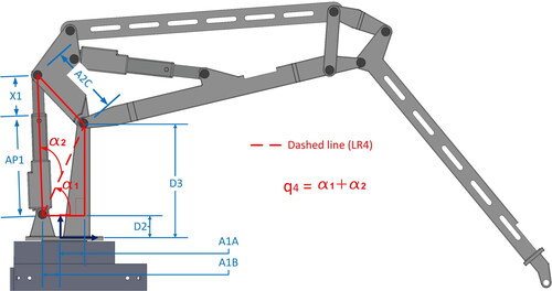
One way to find the kinematic constraints f relating ${\mathbf{q}}_{\mathbf{PA}}$ and ${\mathbf{q}}_{\mathbf{A}}$ is by using trigonometric identities and geometric relations. Figure 6 presents a schematic representation of the forwarder crane that can be used for this purpose. In this figure, $\overline{\text{BD}}$ represents the linear actuator ${\mathrm{A}}_1$ and $\overline{\text{EG}}$ represents the linear actuator ${\mathrm{A}}_2.$ Moreover, the dotted lines are lengths that can be derived from the solid lines, and are useful for obtaining the system equations shown in Eq. (3)(3) $$\mathbf{f}(q_1,X1,X2)=\begin{array}{c}\left(\begin{array}{c}{q}_1\\ {\mathrm{f}}_{{\mathrm{q}}_2}(X1,X2)\\ {\mathrm{f}}_{{\mathrm{q}}_3}(X1,X2)\\ {\mathrm{f}}_{{\mathrm{q}}_4}(X1,X2)\\ X1\\ {\mathrm{f}}_{{\mathrm{q}}_6}(X1,X2)\\ {\mathrm{f}}_{{\mathrm{q}}_7}(X1,X2)\\ {\mathrm{f}}_{{\mathrm{q}}_9}(X1,X2)\\ {\mathrm{f}}_{{\mathrm{q}}_{10}}(X1,X2)\\ X2\\ {\mathrm{f}}_{{\mathrm{q}}_{11}}(X1,X2)\end{array}\right)\end{array}.$$(3) . (3) $$\mathbf{f}(q_1,X1,X2)=\begin{array}{c}\left(\begin{array}{c}{q}_1\\ {\mathrm{f}}_{{\mathrm{q}}_2}(X1,X2)\\ {\mathrm{f}}_{{\mathrm{q}}_3}(X1,X2)\\ {\mathrm{f}}_{{\mathrm{q}}_4}(X1,X2)\\ X1\\ {\mathrm{f}}_{{\mathrm{q}}_6}(X1,X2)\\ {\mathrm{f}}_{{\mathrm{q}}_7}(X1,X2)\\ {\mathrm{f}}_{{\mathrm{q}}_9}(X1,X2)\\ {\mathrm{f}}_{{\mathrm{q}}_{10}}(X1,X2)\\ X2\\ {\mathrm{f}}_{{\mathrm{q}}_{11}}(X1,X2)\end{array}\right)\end{array}.$$(3)

Figure 6. Schematics for trigonometric relationships to transform the dynamic model as a function of the active joints ${\mathbf{q}}_{\mathbf{A}}.$

Finally, Eq. (4)(4) $$\begin{array}{c}{\mathit{\gamma }}^{\mathit{T}}{\mathbf{D}}_{\mathbf{PA}}({\mathbf{q}}_{\mathbf{A}})\mathit{\gamma }\stackrel{..}{{\mathbf{q}}_{\mathbf{A}}}\mathit{+}\hfill \\ {\mathit{\gamma }}^{\mathit{T}}({\mathbf{D}}_{\mathbf{PA}}({\mathbf{q}}_{\mathbf{A}})\dot{\mathit{\gamma }}\mathit{+}{\mathbf{C}}_{\mathbf{PA}}({\mathbf{q}}_{\mathbf{A}},\stackrel{.}{{\mathbf{q}}_{\mathbf{A}}}))\stackrel{.}{{\mathbf{q}}_{\mathbf{A}}}\mathit{+}\hfill \\ {\mathit{\gamma }}^{\mathit{T}}{\mathbf{G}}_{\mathbf{PA}}({\mathbf{q}}_{\mathbf{A}})\mathit{=}{\mathit{\tau }}_{\mathbf{A}},\hfill \\ \mathit{\gamma }=\begin{array}{c}\left(\begin{array}{ccc}1& 0& 0\\ 0& \frac{\partial {\mathrm{f}}_{{\mathrm{q}}_2}(X1,X2)}{\partial X1}& \frac{\partial {\mathrm{f}}_{{\mathrm{q}}_2}(X1,X2)}{\partial X2}\\ 0& \frac{\partial {\mathrm{f}}_{{\mathrm{q}}_3}(X1,X2)}{\partial X1}& \frac{\partial {\mathrm{f}}_{{\mathrm{q}}_3}(X1,X2)}{\partial X2}\\ 0& \frac{\partial {\mathrm{f}}_{{\mathrm{q}}_4}(X1,X2)}{\partial X1}& \frac{\partial {\mathrm{f}}_{{\mathrm{q}}_4}(X1,X2)}{\partial X2}\\ 0& 1& 0\\ 0& \frac{\partial {\mathrm{f}}_{{\mathrm{q}}_6}(X1,X2)}{\partial X1}& \frac{\partial {\mathrm{f}}_{{\mathrm{q}}_6}(X1,X2)}{\partial X2}\\ 0& \frac{\partial {\mathrm{f}}_{{\mathrm{q}}_7}(X1,X2)}{\partial X1}& \frac{\partial {\mathrm{f}}_{{\mathrm{q}}_7}(X1,X2)}{\partial X2}\\ 0& \frac{\partial {\mathrm{f}}_{{\mathrm{q}}_9}(X1,X2)}{\partial X1}& \frac{\partial {\mathrm{f}}_{{\mathrm{q}}_9}(X1,X2)}{\partial X2}\\ 0& \frac{\partial {\mathrm{f}}_{{\mathrm{q}}_{10}}(X1,X2)}{\partial X1}& \frac{\partial {\mathrm{f}}_{{\mathrm{q}}_{10}}(X1,X2)}{\partial X2}\\ 0& 0& 1\\ 0& \frac{\partial {\mathrm{f}}_{{\mathrm{q}}_{11}}(X1,X2)}{\partial X1}& \frac{\partial {\mathrm{f}}_{{\mathrm{q}}_{11}}(X1,X2)}{\partial X2}\end{array}\right)\hfill \end{array}\hfill \end{array}.$$(4) presents the dynamic model of the forwarder crane with closed kinematic chain as a function of the active joints ${\mathbf{q}}_{\mathbf{A}},$ where ${\mathit{\tau }}_{\mathbf{A}}={[{\tau }_1,F_{A1},F_{A2}]}^T,$ τ₁ is the torque exerted by the motor, $F_{A1}$ is the force exerted by the linear actuator ${\mathrm{A}}_1$ and $F_{A2}$ is the force exerted by the linear actuator ${\mathrm{A}}_2.$ An example of how to get the kinematic constraints and their corresponding values in the matrix $\mathit{\gamma }$ is shown in C. The example is focused on the kinematic constraint ${\mathrm{f}}_{{\mathrm{q}}_4}(X1,X2),$ however, the same procedure applies for all other constraints. (4) $$\begin{array}{c}{\mathit{\gamma }}^{\mathit{T}}{\mathbf{D}}_{\mathbf{PA}}({\mathbf{q}}_{\mathbf{A}})\mathit{\gamma }\stackrel{..}{{\mathbf{q}}_{\mathbf{A}}}\mathit{+}\hfill \\ {\mathit{\gamma }}^{\mathit{T}}({\mathbf{D}}_{\mathbf{PA}}({\mathbf{q}}_{\mathbf{A}})\dot{\mathit{\gamma }}\mathit{+}{\mathbf{C}}_{\mathbf{PA}}({\mathbf{q}}_{\mathbf{A}},\stackrel{.}{{\mathbf{q}}_{\mathbf{A}}}))\stackrel{.}{{\mathbf{q}}_{\mathbf{A}}}\mathit{+}\hfill \\ {\mathit{\gamma }}^{\mathit{T}}{\mathbf{G}}_{\mathbf{PA}}({\mathbf{q}}_{\mathbf{A}})\mathit{=}{\mathit{\tau }}_{\mathbf{A}},\hfill \\ \mathit{\gamma }=\begin{array}{c}\left(\begin{array}{ccc}1& 0& 0\\ 0& \frac{\partial {\mathrm{f}}_{{\mathrm{q}}_2}(X1,X2)}{\partial X1}& \frac{\partial {\mathrm{f}}_{{\mathrm{q}}_2}(X1,X2)}{\partial X2}\\ 0& \frac{\partial {\mathrm{f}}_{{\mathrm{q}}_3}(X1,X2)}{\partial X1}& \frac{\partial {\mathrm{f}}_{{\mathrm{q}}_3}(X1,X2)}{\partial X2}\\ 0& \frac{\partial {\mathrm{f}}_{{\mathrm{q}}_4}(X1,X2)}{\partial X1}& \frac{\partial {\mathrm{f}}_{{\mathrm{q}}_4}(X1,X2)}{\partial X2}\\ 0& 1& 0\\ 0& \frac{\partial {\mathrm{f}}_{{\mathrm{q}}_6}(X1,X2)}{\partial X1}& \frac{\partial {\mathrm{f}}_{{\mathrm{q}}_6}(X1,X2)}{\partial X2}\\ 0& \frac{\partial {\mathrm{f}}_{{\mathrm{q}}_7}(X1,X2)}{\partial X1}& \frac{\partial {\mathrm{f}}_{{\mathrm{q}}_7}(X1,X2)}{\partial X2}\\ 0& \frac{\partial {\mathrm{f}}_{{\mathrm{q}}_9}(X1,X2)}{\partial X1}& \frac{\partial {\mathrm{f}}_{{\mathrm{q}}_9}(X1,X2)}{\partial X2}\\ 0& \frac{\partial {\mathrm{f}}_{{\mathrm{q}}_{10}}(X1,X2)}{\partial X1}& \frac{\partial {\mathrm{f}}_{{\mathrm{q}}_{10}}(X1,X2)}{\partial X2}\\ 0& 0& 1\\ 0& \frac{\partial {\mathrm{f}}_{{\mathrm{q}}_{11}}(X1,X2)}{\partial X1}& \frac{\partial {\mathrm{f}}_{{\mathrm{q}}_{11}}(X1,X2)}{\partial X2}\end{array}\right)\hfill \end{array}\hfill \end{array}.$$(4)

2.2.4. Friction forces

The model described by Eq. (4)(4) $$\begin{array}{c}{\mathit{\gamma }}^{\mathit{T}}{\mathbf{D}}_{\mathbf{PA}}({\mathbf{q}}_{\mathbf{A}})\mathit{\gamma }\stackrel{..}{{\mathbf{q}}_{\mathbf{A}}}\mathit{+}\hfill \\ {\mathit{\gamma }}^{\mathit{T}}({\mathbf{D}}_{\mathbf{PA}}({\mathbf{q}}_{\mathbf{A}})\dot{\mathit{\gamma }}\mathit{+}{\mathbf{C}}_{\mathbf{PA}}({\mathbf{q}}_{\mathbf{A}},\stackrel{.}{{\mathbf{q}}_{\mathbf{A}}}))\stackrel{.}{{\mathbf{q}}_{\mathbf{A}}}\mathit{+}\hfill \\ {\mathit{\gamma }}^{\mathit{T}}{\mathbf{G}}_{\mathbf{PA}}({\mathbf{q}}_{\mathbf{A}})\mathit{=}{\mathit{\tau }}_{\mathbf{A}},\hfill \\ \mathit{\gamma }=\begin{array}{c}\left(\begin{array}{ccc}1& 0& 0\\ 0& \frac{\partial {\mathrm{f}}_{{\mathrm{q}}_2}(X1,X2)}{\partial X1}& \frac{\partial {\mathrm{f}}_{{\mathrm{q}}_2}(X1,X2)}{\partial X2}\\ 0& \frac{\partial {\mathrm{f}}_{{\mathrm{q}}_3}(X1,X2)}{\partial X1}& \frac{\partial {\mathrm{f}}_{{\mathrm{q}}_3}(X1,X2)}{\partial X2}\\ 0& \frac{\partial {\mathrm{f}}_{{\mathrm{q}}_4}(X1,X2)}{\partial X1}& \frac{\partial {\mathrm{f}}_{{\mathrm{q}}_4}(X1,X2)}{\partial X2}\\ 0& 1& 0\\ 0& \frac{\partial {\mathrm{f}}_{{\mathrm{q}}_6}(X1,X2)}{\partial X1}& \frac{\partial {\mathrm{f}}_{{\mathrm{q}}_6}(X1,X2)}{\partial X2}\\ 0& \frac{\partial {\mathrm{f}}_{{\mathrm{q}}_7}(X1,X2)}{\partial X1}& \frac{\partial {\mathrm{f}}_{{\mathrm{q}}_7}(X1,X2)}{\partial X2}\\ 0& \frac{\partial {\mathrm{f}}_{{\mathrm{q}}_9}(X1,X2)}{\partial X1}& \frac{\partial {\mathrm{f}}_{{\mathrm{q}}_9}(X1,X2)}{\partial X2}\\ 0& \frac{\partial {\mathrm{f}}_{{\mathrm{q}}_{10}}(X1,X2)}{\partial X1}& \frac{\partial {\mathrm{f}}_{{\mathrm{q}}_{10}}(X1,X2)}{\partial X2}\\ 0& 0& 1\\ 0& \frac{\partial {\mathrm{f}}_{{\mathrm{q}}_{11}}(X1,X2)}{\partial X1}& \frac{\partial {\mathrm{f}}_{{\mathrm{q}}_{11}}(X1,X2)}{\partial X2}\end{array}\right)\hfill \end{array}\hfill \end{array}.$$(4) does not consider friction forces, however, they should be taken into account to experimentally validate the model. In general, friction forces in real systems oppose motion, have considerable asymmetric patterns and depend on velocities and motion direction (Glocker 2013). In this work, we consider a friction model often used for mechanical systems, which combines Coulomb and viscous frictions (Olsson et al. 1998). In addition, it is noteworthy that this friction model has already been used to validate friction forces in industrial-size forestry cranes (La Hera and Ortiz Morales 2014). The friction forces vector (${\mathbf{F}}_{\mathbf{F}}$) is mathematically stated as, (5) $$\begin{array}{c}{\mathbf{F}}_{\mathbf{F}}={\mathbf{F}}_{{\mathbf{F}}_{\mathbf{qA}}}+{\mathbf{F}}_{{\mathbf{F}}_{\mathbf{qPA}}},\hfill \\ {\mathbf{F}}_{{\mathbf{F}}_{\mathbf{qA}}}=\begin{array}{c}\left(\begin{array}{c}{F}_{C_{q1}}s\mathit{ign}(\stackrel{.}{q_1})+{\Delta }_{C_{q1}}+F_{V_{q1}}\stackrel{.}{q_1}+{\Delta }_{V_{q1}}\left|\stackrel{.}{q_1}\right|\\ F_{C_{X1}}s\mathit{ign}(\stackrel{.}{X1})+{\Delta }_{C_{X1}}+F_{V_{X1}}\stackrel{.}{X1}+{\Delta }_{V_{X1}}\left|\stackrel{.}{X1}\right|\\ F_{C_{X2}}s\mathit{ign}(\stackrel{.}{X2})+{\Delta }_{C_{X2}}+F_{V_{X2}}\stackrel{.}{X2}+{\Delta }_{V_{X2}}\left|\stackrel{.}{X2}\right|\end{array}\right)\hfill \end{array},\hfill \\ {\mathbf{F}}_{{\mathbf{F}}_{\mathbf{qPA}}}={\mathit{\gamma }}^{\mathit{T}}{\mathit{\mu }}_{\mathit{\nu }}\mathit{\gamma }\stackrel{.}{{\mathbf{q}}_{\mathbf{A}}}.\hfill \end{array}$$(5)

In Eq. (5)(5) $$\begin{array}{c}{\mathbf{F}}_{\mathbf{F}}={\mathbf{F}}_{{\mathbf{F}}_{\mathbf{qA}}}+{\mathbf{F}}_{{\mathbf{F}}_{\mathbf{qPA}}},\hfill \\ {\mathbf{F}}_{{\mathbf{F}}_{\mathbf{qA}}}=\begin{array}{c}\left(\begin{array}{c}{F}_{C_{q1}}s\mathit{ign}(\stackrel{.}{q_1})+{\Delta }_{C_{q1}}+F_{V_{q1}}\stackrel{.}{q_1}+{\Delta }_{V_{q1}}\left|\stackrel{.}{q_1}\right|\\ F_{C_{X1}}s\mathit{ign}(\stackrel{.}{X1})+{\Delta }_{C_{X1}}+F_{V_{X1}}\stackrel{.}{X1}+{\Delta }_{V_{X1}}\left|\stackrel{.}{X1}\right|\\ F_{C_{X2}}s\mathit{ign}(\stackrel{.}{X2})+{\Delta }_{C_{X2}}+F_{V_{X2}}\stackrel{.}{X2}+{\Delta }_{V_{X2}}\left|\stackrel{.}{X2}\right|\end{array}\right)\hfill \end{array},\hfill \\ {\mathbf{F}}_{{\mathbf{F}}_{\mathbf{qPA}}}={\mathit{\gamma }}^{\mathit{T}}{\mathit{\mu }}_{\mathit{\nu }}\mathit{\gamma }\stackrel{.}{{\mathbf{q}}_{\mathbf{A}}}.\hfill \end{array}$$(5) , ${\mathbf{F}}_{{\mathbf{F}}_{\mathbf{qA}}}$ is the friction forces vector in the actuators (related to the active joints), which considers asymmetric Coulomb and viscous frictions. ${\mathbf{F}}_{{\mathbf{F}}_{\mathbf{qPA}}}$ is the friction forces vector in the passive joints, where only viscous friction forces are taken into account. Coulomb friction forces are considered only in the active joints due to the gearboxes’ dynamic effects. Coulomb friction mean values for the motor, the linear actuator ${\mathrm{A}}_1$ and the linear actuator ${\mathrm{A}}_2$ are $F_{C_{q1}},F_{C_{X1}}$ and $F_{C_{X2}}$ respectively, while ${\Delta }_{C_{q1}},{\Delta }_{C_{X1}},{\Delta }_{C_{X2}}$ represent the variational coefficients. Viscous friction mean values for the motor, the linear actuator ${\mathrm{A}}_1$ and the linear actuator ${\mathrm{A}}_2$ are $F_{V_{q1}},F_{V_{X1}}$ and $F_{V_{X2}}$ respectively, while ${\Delta }_{V_{q1}},{\Delta }_{V_{X1}},{\Delta }_{V_{X2}}$ represent the variational coefficients. Finally, ${\mathit{\mu }}_{\mathit{\nu }}$ represents the diagonal matrix containing viscous friction coefficients. Specific values used for the experimental validation are shown in Table 1.

Table 1. Physical parameters used for friction forces, controller gains, and relations force/torque-current.

Friction coefficients for ${\mathit{\mu }}_{\mathit{\nu }}$ (${\mathrm{q}}_1,\dots ,{\mathrm{q}}_{11}$)
(a)
Parameter	Value	Unit
${\mu }_{{\nu }_{q1}}$	0.8	kg ${\mathrm{m}}^2$/s
${\mu }_{{\nu }_i},{\mathrm{i}=\mathrm{q}}_2,\dots ,{\mathrm{q}}_{11}$	0.4	kg ${\mathrm{m}}^2$/s
${\mu }_{{\nu }_{i2}},\mathrm{i}2=\mathrm{X}1,\mathrm{X}2$	0.4	kg /s
Values for ${\mathit{F}}_{\mathit{C}}$
Parameter	Value	Unit
$F_{C_{q1}}$	−0.1010	N m
${\Delta }_{C_{q1}}$	−0.0110	N m
$F_{V_{q1}}$	0	kg ${\mathrm{m}}^2$/s
${\Delta }_{V_{q1}}$	0	kg ${\mathrm{m}}^2$/s
$F_{C_{X1}}$	−16	N
${\Delta }_{C_{X1}}$	6	N
$F_{V_{X1}}$	−600	kg/s
${\Delta }_{V_{X1}}$	0	kg/s
$F_{C_{X2}}$	−7.5	N
${\Delta }_{C_{X2}}$	−21.5	N
$F_{V_{X2}}$	−500	kg/s
${\Delta }_{V_{X2}}$	300	kg/s
(b)
PI Controller Gains
Gains motor	Gains A1	Gains A2
$K_{p_1}=15$	$K_{p_2}=5500$	$K_{p_2}=18000$
$K_{i_1}=5$	$K_{i_2}=19500$	$K_{i_3}=20000$
Constants for force-current and torque-current
Parameter	Value	Unit
Px	1.765	N-m
Cy	1.5	A
b	0.050	A
Fx	20	N
Cx	0.050	A

By combining Eqs. (4)(4) $$\begin{array}{c}{\mathit{\gamma }}^{\mathit{T}}{\mathbf{D}}_{\mathbf{PA}}({\mathbf{q}}_{\mathbf{A}})\mathit{\gamma }\stackrel{..}{{\mathbf{q}}_{\mathbf{A}}}\mathit{+}\hfill \\ {\mathit{\gamma }}^{\mathit{T}}({\mathbf{D}}_{\mathbf{PA}}({\mathbf{q}}_{\mathbf{A}})\dot{\mathit{\gamma }}\mathit{+}{\mathbf{C}}_{\mathbf{PA}}({\mathbf{q}}_{\mathbf{A}},\stackrel{.}{{\mathbf{q}}_{\mathbf{A}}}))\stackrel{.}{{\mathbf{q}}_{\mathbf{A}}}\mathit{+}\hfill \\ {\mathit{\gamma }}^{\mathit{T}}{\mathbf{G}}_{\mathbf{PA}}({\mathbf{q}}_{\mathbf{A}})\mathit{=}{\mathit{\tau }}_{\mathbf{A}},\hfill \\ \mathit{\gamma }=\begin{array}{c}\left(\begin{array}{ccc}1& 0& 0\\ 0& \frac{\partial {\mathrm{f}}_{{\mathrm{q}}_2}(X1,X2)}{\partial X1}& \frac{\partial {\mathrm{f}}_{{\mathrm{q}}_2}(X1,X2)}{\partial X2}\\ 0& \frac{\partial {\mathrm{f}}_{{\mathrm{q}}_3}(X1,X2)}{\partial X1}& \frac{\partial {\mathrm{f}}_{{\mathrm{q}}_3}(X1,X2)}{\partial X2}\\ 0& \frac{\partial {\mathrm{f}}_{{\mathrm{q}}_4}(X1,X2)}{\partial X1}& \frac{\partial {\mathrm{f}}_{{\mathrm{q}}_4}(X1,X2)}{\partial X2}\\ 0& 1& 0\\ 0& \frac{\partial {\mathrm{f}}_{{\mathrm{q}}_6}(X1,X2)}{\partial X1}& \frac{\partial {\mathrm{f}}_{{\mathrm{q}}_6}(X1,X2)}{\partial X2}\\ 0& \frac{\partial {\mathrm{f}}_{{\mathrm{q}}_7}(X1,X2)}{\partial X1}& \frac{\partial {\mathrm{f}}_{{\mathrm{q}}_7}(X1,X2)}{\partial X2}\\ 0& \frac{\partial {\mathrm{f}}_{{\mathrm{q}}_9}(X1,X2)}{\partial X1}& \frac{\partial {\mathrm{f}}_{{\mathrm{q}}_9}(X1,X2)}{\partial X2}\\ 0& \frac{\partial {\mathrm{f}}_{{\mathrm{q}}_{10}}(X1,X2)}{\partial X1}& \frac{\partial {\mathrm{f}}_{{\mathrm{q}}_{10}}(X1,X2)}{\partial X2}\\ 0& 0& 1\\ 0& \frac{\partial {\mathrm{f}}_{{\mathrm{q}}_{11}}(X1,X2)}{\partial X1}& \frac{\partial {\mathrm{f}}_{{\mathrm{q}}_{11}}(X1,X2)}{\partial X2}\end{array}\right)\hfill \end{array}\hfill \end{array}.$$(4) and (5)(5) $$\begin{array}{c}{\mathbf{F}}_{\mathbf{F}}={\mathbf{F}}_{{\mathbf{F}}_{\mathbf{qA}}}+{\mathbf{F}}_{{\mathbf{F}}_{\mathbf{qPA}}},\hfill \\ {\mathbf{F}}_{{\mathbf{F}}_{\mathbf{qA}}}=\begin{array}{c}\left(\begin{array}{c}{F}_{C_{q1}}s\mathit{ign}(\stackrel{.}{q_1})+{\Delta }_{C_{q1}}+F_{V_{q1}}\stackrel{.}{q_1}+{\Delta }_{V_{q1}}\left|\stackrel{.}{q_1}\right|\\ F_{C_{X1}}s\mathit{ign}(\stackrel{.}{X1})+{\Delta }_{C_{X1}}+F_{V_{X1}}\stackrel{.}{X1}+{\Delta }_{V_{X1}}\left|\stackrel{.}{X1}\right|\\ F_{C_{X2}}s\mathit{ign}(\stackrel{.}{X2})+{\Delta }_{C_{X2}}+F_{V_{X2}}\stackrel{.}{X2}+{\Delta }_{V_{X2}}\left|\stackrel{.}{X2}\right|\end{array}\right)\hfill \end{array},\hfill \\ {\mathbf{F}}_{{\mathbf{F}}_{\mathbf{qPA}}}={\mathit{\gamma }}^{\mathit{T}}{\mathit{\mu }}_{\mathit{\nu }}\mathit{\gamma }\stackrel{.}{{\mathbf{q}}_{\mathbf{A}}}.\hfill \end{array}$$(5) , the dynamic model of the forwarder crane with closed kinematic chain can be formulated as, (6) $$\begin{array}{c}{\mathit{\gamma }}^{\mathit{T}}{\mathbf{D}}_{\mathbf{PA}}({\mathbf{q}}_{\mathbf{A}})\mathit{\gamma }\stackrel{..}{{\mathbf{q}}_{\mathbf{A}}}\mathit{+}\hfill \\ {\mathit{\gamma }}^{\mathit{T}}({\mathbf{D}}_{\mathbf{PA}}({\mathbf{q}}_{\mathbf{A}})\dot{\mathit{\gamma }}\mathit{+}{\mathbf{C}}_{\mathbf{PA}}({\mathbf{q}}_{\mathbf{A}},\stackrel{.}{{\mathbf{q}}_{\mathbf{A}}}))\stackrel{.}{{\mathbf{q}}_{\mathbf{A}}}\mathit{+}\hfill \\ {\mathit{\gamma }}^{\mathit{T}}{\mathbf{G}}_{\mathbf{PA}}({\mathbf{q}}_{\mathbf{A}})\mathit{+}{\mathbf{F}}_{\mathbf{F}}\mathit{=}{\mathit{\tau }}_{\mathbf{A}}.\hfill \end{array}$$(6)

2.3. Closed-loop control

Experimental validation is done through three tests, where the end-effector (the point described by distance A7 in Fig. 11b) should follow a reference trajectory.

These reference trajectories are given in Cartesian coordinates, implying that a transformation to the joint coordinate space is needed. This transformation is done by considering the end-effector and the inverse kinematics of chain A. After $q_1,q_2,$ and $q_3$ are known, a second transformation is needed. The second transformation is performed by geometric relations and aims to derive the desired values of $q_1,$ X1, and X2. Since it is necessary to assure that the end-effector follows the trajectory and that the actuators perform the desired movements, closed-loop control is needed.

For the closed-loop control, we consider three PI controllers (one per actuator). The control model is stated as follows, (7) $${\mathit{\tau }}_{\mathbf{A}}\mathit{=}\begin{array}{c}\left(\begin{array}{c}{K}_{p_1}{e}_{q1}+K_{i_1}\int e_{q1}dt\\ K_{p_2}{e}_{X1}+K_{i_2}\int e_{X1}dt\\ K_{p_3}{e}_{X2}+K_{i_3}\int e_{X2}dt\end{array}\right)\end{array}.$$(7)

In Eq. (7)(7) $${\mathit{\tau }}_{\mathbf{A}}\mathit{=}\begin{array}{c}\left(\begin{array}{c}{K}_{p_1}{e}_{q1}+K_{i_1}\int e_{q1}dt\\ K_{p_2}{e}_{X1}+K_{i_2}\int e_{X1}dt\\ K_{p_3}{e}_{X2}+K_{i_3}\int e_{X2}dt\end{array}\right)\end{array}.$$(7) , $K_{p_1},K_{p_2},$ and $K_{p_3}$ represent coefficients of proportional terms for the motor, the linear actuator ${\mathrm{A}}_1,$ and the linear actuator ${\mathrm{A}}_2$ respectively, while $K_{i_1},K_{i_2},$ and $K_{i_3}$ represent coefficients of integral terms. Finally, position errors are $e_{q1}=q_{1d}-q_1,e_{X1}=X{1}_d-X1$ and $e_{X2}=X{2}_d-X2,$ with $q_{1d},X{1}_d$ and $X{2}_d$ as the desired position values for the motor, the linear actuator ${\mathrm{A}}_1$ and the linear actuator ${\mathrm{A}}_2,$ respectively. The closed-loop controller is implemented in both, simulation and real hardware (Table 1). Figure 7 shows a block diagram of the controllers operating principle.

Figure 7. Block diagram for closed-loop control of the forwarder crane.

2.4. Force-current and Torque-current relations

As mentioned in Section 2.1, our experimental validation considers a comparison between simulated values and experimental values of forces and torques. To carry out this comparison, it is necessary to compute the experimental values of the torque and forces from the current measured in these devices. The mathematical expressions used for this purpose are the following: (8) $$\begin{array}{c}{\tau }_{1\hspace{0.17em}\text{exp}\hspace{0.17em}}=(I_{mo})\frac{P_X}{C_Y},\\ {\mathrm{F}}_{\text{Aexp}}=(I_{la}-b)\frac{F_X}{C_X},\end{array}$$(8) where ${\tau }_{1\hspace{0.17em}\text{exp}\hspace{0.17em}}$ is the motor’s torque, I_mo is the current measured in the motor, while P_X and C_Y are proportionality constants obtained from data sheets of the manufacturer. For the linear actuators ${\mathrm{A}}_1$ and ${\mathrm{A}}_2,{\mathrm{F}}_{\text{Aexp}}$ represents the actuator force, I_la is the current measured in either of both actuators, while b, F_X and C_X are again proportionality constants obtained from data sheets of the manufacturer.

2.5. Physical parameters and modelling error

Physical parameter values used for experimental validation are shown in Tables 1 and 4. Table 1(a) shows parameter values for the friction coefficients, which were selected through experimental tests and typical friction values for steel/steel and steel/bronze contacts. Table 1(b) shows first the PI controller gain values defined by Eq. (7)(7) $${\mathit{\tau }}_{\mathbf{A}}\mathit{=}\begin{array}{c}\left(\begin{array}{c}{K}_{p_1}{e}_{q1}+K_{i_1}\int e_{q1}dt\\ K_{p_2}{e}_{X1}+K_{i_2}\int e_{X1}dt\\ K_{p_3}{e}_{X2}+K_{i_3}\int e_{X2}dt\end{array}\right)\end{array}.$$(7) and second, it presents the force-current and torque-current constants for the mathematical relations stated in Eq. (8)(8) $$\begin{array}{c}{\tau }_{1\hspace{0.17em}\text{exp}\hspace{0.17em}}=(I_{mo})\frac{P_X}{C_Y},\\ {\mathrm{F}}_{\text{Aexp}}=(I_{la}-b)\frac{F_X}{C_X},\end{array}$$(8) . Parameters in Table 4 correspond to the lengths and masses shown in Fig. 11 and were taken from CAD models.

Table 4. Physical parameters used for comparison between experimental and simulation results.

(a)
Link 1 – Chain A
Parameter	Value	Unit
D2	0.017	m
D3	0.087	m
A1A	0.015	m
A1B	0.017	m
PCX1	0.0087	m
PCZ1	0.0032	m
M1	0.3181	kg
I1	0.0782	gr / ${\mathrm{m}}^3$
(b)
Link 3 – Chain A
Parameter	Value	Unit
A3	0.2200	m
A31X	0.195	m
α10	0.0181	rad
α11	0.0205	rad
PCX3	0.11	m
PCZ3	0.0109	m
M3	0.218	kg
I3	3.0823	gr / ${\mathrm{m}}^3$
(c)
Link 7 – Chain A
Parameter	Value	Unit
A7	0.2220	m
PCX7	0.1061	m
PCY7	0.00025	m
M7	0.218	kg
I7	3.0944	gr / ${\mathrm{m}}^3$
(d)
Link 4 – Chain B
Parameter	Value	Unit
A4	0.205	m
PCX4	0.1025	m
PCY4	0	m
M4	0.201	kg
I4	2.9254	gr / ${\mathrm{m}}^3$
(e)
Link 6 – Chain B
Parameter	Value	Unit
A6	0.0431	m
PCX6	0.02	m
PCY6	0.008	m
M6	0.053	kg
I6	0.03158	gr / ${\mathrm{m}}^3$
(f)
Link 2 – Chain C
Parameter	Value	Unit
A2	0.072	m
A2B	0.0424	m
A2C	0.0516	m
A2D	0.050	m
PCX2	0.0364	m
PCY2	0.0104	m
M2	0.1833	kg
I2	0.00817	gr / ${\mathrm{m}}^3$
(g)
Link 5 – Chain D
Parameter	Value	Unit
A5	0.045	m
PCX5	0.0225	m
PCY5	0	m
M5	0.0280	kg
I5	0.0174	gr / ${\mathrm{m}}^3$
(h)
Linear Actuators
Parameter	Value	Unit
AP1/AP2	0.0825	m
PCXP1/PCXP2	0.04	m
${\mathrm{K}}_{\mathrm{m}}$	0.19	–

2.5.1. Percentage error

The comparison measure (modeling error) between experimental results and simulation results is the percentage error, which refers to the difference between the experimental force vector and the simulated force vector when performing a particular task. Percentage errors for τ₁, $F_{A1}$ and $F_{A2}$ are calculated by the following expression, (9) $$\begin{array}{c}{I}_{VD}={\int }_0^{t_f}{V}_{D}dt,\\ I_{VE}={\int }_0^{t_f}{V}_{E}dt,\\ {\text{PE}}_{{\tau }_1,\text{FA}1,\text{FA}2}=\frac{I_{VD}}{I_{VE}}\times 100.\end{array}$$(9)

For the percentage error of τ₁, $V_D={({\tau }_{1\hspace{0.17em}\mathit{\text{exp}}\hspace{0.17em}}-{\tau }_1)}^2$ and $V_E={({\tau }_{1\hspace{0.17em}\mathit{\text{exp}}\hspace{0.17em}})}^2.$ For the percentage error of $F_{A1},V_D={(F_{A1\hspace{0.17em}\mathit{\text{exp}}\hspace{0.17em}}-F_{A1})}^2$ and $V_E={(F_{A1\hspace{0.17em}\mathit{\text{exp}}\hspace{0.17em}})}^2.$ Finally, for ${\text{PE}}_{\text{FA}2},V_D={(F_{A2\hspace{0.17em}\mathit{\text{exp}}\hspace{0.17em}}-F_{A2})}^2$ and $V_E={(F_{A2\hspace{0.17em}\mathit{\text{exp}}\hspace{0.17em}})}^2.$ The fourth-order Runge-Kutta method was used as integration method for the numerical simulations.

3. Experimental validation and results

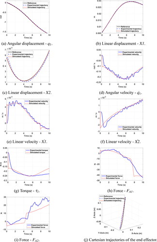
3.1. Trajectory 1

This trajectory is intended to represent a loading task in forwarding operations, where a log is picked up and placed into a log-bunk. For both cases, simulation and experimental results, the crane’s motion starts from rest while the parametric equations for this path are shown in Eq. (10)(10) $$\begin{array}{ccc}{\mathrm{X}}_{\mathrm{r}}& =& -0.004477t^2+0.07305t\\ {\mathrm{Y}}_{\mathrm{r}}& =& 4.7260\times {10}^{-5}{t}^2+0.02643t-0.2676\\ {\mathrm{Z}}_{\mathrm{r}}& =& 2.6490\times {10}^{-5}{t}^2+0.01482t-0.0521\end{array}.$$(10) . Units for ${\mathrm{X}}_{\mathrm{r}},{\mathrm{Y}}_{\mathrm{r}}$ and ${\mathrm{Z}}_{\mathrm{r}}$ are expressed in meters and $0\le t\le 10$ s. (10) $$\begin{array}{ccc}{\mathrm{X}}_{\mathrm{r}}& =& -0.004477t^2+0.07305t\\ {\mathrm{Y}}_{\mathrm{r}}& =& 4.7260\times {10}^{-5}{t}^2+0.02643t-0.2676\\ {\mathrm{Z}}_{\mathrm{r}}& =& 2.6490\times {10}^{-5}{t}^2+0.01482t-0.0521\end{array}.$$(10)

Figure 8 shows experimental and simulation results for trajectory 1. Figures 8(a)–8(c) show displacements of $q_1,X1$ and $X2$ respectively, while Figs. 8(d)–8(f) show velocities $\stackrel{.}{q_1},\stackrel{.}{X1}$ and $\stackrel{.}{X2}$ respectively. The motor torque is shown in Fig. 8(g), the force of the linear actuator ${\mathrm{A}}_1$ is shown in Fig. 8(h) and the force of the linear actuator ${\mathrm{A}}_2$ is shown in Fig. 8(i). Finally, Cartesian trajectories of the end-effector are shown in Fig. 8(j), while the modeling percentage errors can be seen in Table 2. For this trajectory, the order of magnitude of the linear displacement $X1$ is greater than that of the linear displacement $X2,$ however, order of magnitudes of the linear velocities are the same. When analyzing the linear velocity $\stackrel{.}{X1},$ it can be seen that from second 2 to second 8, $\stackrel{.}{X1}$ oscillates without abrupt changes around $-2x{10}^{-3}\mathrm{m}/\mathrm{s}.$ This effect can be seen in the force $F_{A1},$ since from second 2 there are no abrupt changes in the force magnitude.

Figure 8. Displacements, velocities, torques and Cartesian representation for Trajectory 1.

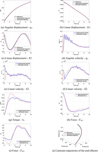
Table 2. Modeling percentage errors.

Trajectory 1
—	IV D	IV E	Units	Percentage error
${\text{PE}}_{{\tau }_1}$	0.0023	0.0867	${\mathrm{N}}^2$ ${\mathrm{m}}^2$ s	2.65 %
${\text{PE}}_{\text{FA}1}$	10.1685	3101.10	${\mathrm{N}}^2$ s	0.32 %
${\text{PE}}_{\text{FA}2}$	23.3439	411.216	${\mathrm{N}}^2$ s	5.67 %
Trajectory 2
—	IV D	IV E	Units	Percentage error
${\text{PE}}_{{\tau }_1}$	0.0133	0.5133	${\mathrm{N}}^2$ ${\mathrm{m}}^2$ s	2.59 %
${\text{PE}}_{\text{FA}1}$	235.0016	3424.60	${\mathrm{N}}^2$ s	6.86 %
${\text{PE}}_{\text{FA}2}$	369.0757	2564.90	${\mathrm{N}}^2$ s	14.37 %
Trajectory 3
—	IV D	IV E	Units	Percentage error
${\text{PE}}_{{\tau }_1}$	0	0	${\mathrm{N}}^2$ ${\mathrm{m}}^2$ s	0 %
${\text{PE}}_{\text{FA}1}$	51.4743	15574.05	${\mathrm{N}}^2$ s	0.3305 %
${\text{PE}}_{\text{FA}2}$	55.9491	373.93	${\mathrm{N}}^2$ s	14.960 %

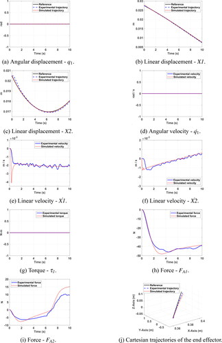
3.2. Trajectory 2

This trajectory represents a move back to the logs loading area. The crane’s motion starts in the ending point of trajectory 1, that is, in the Cartesian coordinates (0.2828 m, 0.0014 m, 0.0987 m), while its motion finishes in the Cartesian coordinates (-0.0189 m, −0.2676 m, −0.0426 m). Eq. (11)(11) $$\begin{array}{ccc}{\mathrm{X}}_{\mathrm{r}}& =& -5.2980\times {10}^{-5}{t}^2-0.02964t+0.2828\\ {\mathrm{Y}}_{\mathrm{r}}& =& -4.7260\times {10}^{-5}{t}^2-0.02643t+0.0014\\ {\mathrm{Z}}_{\mathrm{r}}& =& 0.002239t^2-0.03652t+0.09873\end{array}.$$(11) shows the parametric equations, where units are expressed in meters and $0\le t\le 10$ s. (11) $$\begin{array}{ccc}{\mathrm{X}}_{\mathrm{r}}& =& -5.2980\times {10}^{-5}{t}^2-0.02964t+0.2828\\ {\mathrm{Y}}_{\mathrm{r}}& =& -4.7260\times {10}^{-5}{t}^2-0.02643t+0.0014\\ {\mathrm{Z}}_{\mathrm{r}}& =& 0.002239t^2-0.03652t+0.09873\end{array}.$$(11)

For trajectory 2, experimental and simulation results are shown in Fig. 9. Displacements of $q_1,X1$ and $X2$ are shown in Figs. 9(a)–9(c) respectively. Velocities $\stackrel{.}{q_1},\stackrel{.}{X1}$ and $\stackrel{.}{X2}$ are presented in Figs. 9(d)–9(f) respectively. The motor torque is shown in Fig. 9(g), the force of the linear actuator ${\mathrm{A}}_1$ is shown in Fig. 9(h) and the force of the linear actuator ${\mathrm{A}}_2$ is shown in Fig. 9(i). Cartesian trajectories of the end-effector are shown in Fig. 9(j), and the percentage errors are shown in Table 2. For trajectory 2, once again, the order of magnitude of the linear displacement of $X1$ is greater than that of the linear displacement of $X2$ and order of magnitudes of the linear velocities are the same. When analyzing linear displacements $X1$ and $X2$ can be noticed that there are motion direction changes when performing the task. For $X1,$ this change occurs around second 7, while for $X2$ occurs around second 4. This motion direction changes are easier to identify in the simulated velocities, since simulations show abrupt velocity changes.

Figure 9. Displacements, velocities, torques and Cartesian representation for Trajectory 2.

3.3. Trajectory 3

The last trajectory aims to perform a straight line in the Cartesian space. For this path, the crane’s motion starts in the Cartesian coordinates (0.37439 m, 0 m, −0.06156 m) and finishes in the Cartesian coordinates (0.3882 m, 0 m, 0.1307 m). The parametric equations for the third path are shown in Eq. (12)(12) $$\begin{array}{ccc}{\mathrm{X}}_{\mathrm{r}}& =& 0.00138t+0.37439\\ {\mathrm{Y}}_{\mathrm{r}}& =& 0\\ {\mathrm{Z}}_{\mathrm{r}}& =& 0.01923t-0.06156\end{array}.$$(12) , where units are expressed in meters and $0\le t\le 10$ s. (12) $$\begin{array}{ccc}{\mathrm{X}}_{\mathrm{r}}& =& 0.00138t+0.37439\\ {\mathrm{Y}}_{\mathrm{r}}& =& 0\\ {\mathrm{Z}}_{\mathrm{r}}& =& 0.01923t-0.06156\end{array}.$$(12)

For the last trajectory, experimental and simulation results are shown in Fig. 10. Displacements $q_1,X1$ and $X2$ are shown in Figs. 10(a)–10(c) respectively. Velocities $\stackrel{.}{q_1},\stackrel{.}{X1}$ and $\stackrel{.}{X2}$ are presented in Figs. 10(d)–10(f) respectively. The motor torque and the linear actuators A₁ and A₂ forces are shown in Figs. 10(g)–10(i), respectively. Finally, the Cartesian trajectories of the end-effector are shown in Fig. 10(j), while the percentage errors can be seen in Table 2. For trajectory 3, order of magnitudes of linear displacements are the same. When comparing linear displacement $X1$ and velocity $\stackrel{.}{X1}$ of trajectory 3 with $X1$ and $\stackrel{.}{X1}$ of trajectory 1, it can be seen that the behaviors are similar, which is verified by comparing the forces $F_{A1},$ which also coincide in magnitude and behavior pattern. For the case of displacement $X2,$ it can be seen that around second 6, there is a change in the motion direction. This change is reflected to a greater extent in force $F_{A2},$ since an abrupt change in the behavior pattern can be appreciated.

Figure 10. Displacements, velocities, torques and Cartesian representation for Trajectory 3.

In general, the results presented in this section show that experimental and simulation results have the same patterns of displacement, velocity and force, while all percentage errors are below 15%. The largest values for percentage errors are for the linear actuator ${\mathrm{A}}_2$ when performing trajectories 2 and 3. It is noteworthy that percentage error values depend mainly on two factors. First, we consider ideal or approximated values of masses, inertias, lengths and frictions in simulations, but actual values in the experimental platform are different. There exist different methods to carry out the system identification that would help reduce the gap between experimental and simulation results (Ljung 1999), nevertheless, detailed system identification of the CKC is considered for future work. Second, experimental torque and forces are computed through Eq. (8)(8) $$\begin{array}{c}{\tau }_{1\hspace{0.17em}\text{exp}\hspace{0.17em}}=(I_{mo})\frac{P_X}{C_Y},\\ {\mathrm{F}}_{\text{Aexp}}=(I_{la}-b)\frac{F_X}{C_X},\end{array}$$(8) , which represents only an approximation of the real force and torque values. In addition, Eq. (8)(8) $$\begin{array}{c}{\tau }_{1\hspace{0.17em}\text{exp}\hspace{0.17em}}=(I_{mo})\frac{P_X}{C_Y},\\ {\mathrm{F}}_{\text{Aexp}}=(I_{la}-b)\frac{F_X}{C_X},\end{array}$$(8) uses the current measured to compute these values. In our experimental platform we use a circuit based on low impedance resistors, where the electronic components have a tolerance between 5% and 10%, implying that the values for the current are not 100% accurate.

Moreover, we considered only one set of gains for all experiments, where gain values for the PI controllers of the linear actuators ${\mathrm{A}}_1$ and ${\mathrm{A}}_2$ are greater than the gain values of the PI controller of the motor. First, these values are tuned so that all trajectories can be carried out without the need to modify those values. Nevertheless, different controller gain values can be tuned accordingly to the particular tasks. Second, it is noteworthy that differences between the gain values are because the dynamics of linear and rotational actuators are different, which implies that different values and ranges must be taken into account, as shown in Table 1.

4. General discussion

Although the design is a crucial aspect in the performance of a mechanical system, very little has been done to understand how new forestry crane designs could influence the performance of such machines. On the contrary, manufacturers of forestry cranes have chosen to produce heavier and larger machines (in addition to automation technology) to cope with the demands of higher productivity made by the market. This approach has produced acceptable results in general terms, however, it is impractical to keep making cranes bigger, when the current situation is that these machines bring several complications: they are difficult to operate, provoke ground damage, demand high amounts of fuel to operate, have high vibration levels and make the implementation of automation technology difficult. Hence, these machines are not efficient and have kept tree harvesting productivity in Nordic countries stagnated for decades.

Considering the current state-of-the-art, it is necessary to start looking for different options to improve forestry cranes’ performance rather than continuing the traditional pathway of development. Model-based design has proven to be a powerful approach to improve performance in many systems by modifying their base design. It is well known that by modifying the inertial and kinematic terms of a system, the dynamic system performance will inevitably change. This is the main idea behind model-based design, to modify certain parameters to improve one or many performance criteria. In addition, the model-based design approach opens even greater opportunities to improve forestry cranes’ performance. For instance, by combining model-based design, gravity compensation and mathematical optimization, we can expect significant improvements in energy consumption, dexterity of human operators, ground damage and reduction of ${\text{CO}}_2$ emissions. However, as mentioned in the introduction of this article, the success of this design approach depends on how well the model is stated and the elements that are taken into account in the model. For this reason, it is important to consider the closed-kinematic chain in the model, since there are more elements and dynamic effects that can be used to improve forestry cranes performance. Also, it is important to remember that redesigning starts by understanding the dynamic behavior of the system.

On the other hand, one of the main challenges for many industries when testing new technology or designs is to reduce the cost-benefit ratio. For forestry crane manufacturers (particularly small or medium size companies), taking a high risk is not feasible, since they can afford to lose millions if the design or technology does not succeed. By using reduced-scale prototypes, this high risk investment reduces considerably. To have a clear idea of the costs, it is important to mention that the total amount spent for the prototype in this work was less than 8000 €, so the cost-benefit ratio reduced at least 10 times if we consider that the cost for prototyping an industrial size crane (considering a conservative estimation) would be around 80 000 €.

Finally, it is noteworthy that the experimental platform and the model in this work broaden the options not only to design or sketch new concepts, designs and algorithms of forestry cranes, but also to other similar heavy-duty machinery.

5. Conclusions

In this article, a reduced-scale platform for testing new designs, components and/or algorithms in forestry cranes and the dynamic model of a reduced-scale forwarder crane with a closed kinematic chain are presented.

The reduced-scale experimental platform considered a rapid manufacturing process via metal 3 D printing technology. By using 3 D printing, the prototyping process speeds up, as it is possible to 3 D print objects in a few hours, which is much faster than molded or machined parts. Furthermore, it allows each design modification to be completed at a much more efficient rate. In addition, this platform has different components which are similar to those of a real size crane, that is, sensors, linear actuators, motors, processing units and control algorithms. The only component that is excluded in this platform is the hydraulic system, nevertheless, how to model and consider the dynamics of a hydraulic system in a forestry crane has been previously presented (La Hera and Ortiz Morales 2014).

Moreover, the dynamic model presented in this article reduces the knowledge gap on model-based design of forestry cranes, since the closed kinematic chains (which are common in forestry cranes) had not been previously taken into account. The procedure to derive the equations describing the crane’s dynamics consider a system of multiple open kinematic chains as functions of the active variable joints. In addition to the dynamic model, the experimental validation is also presented. The experimental validation is performed by means of three tests. The first test considers that the forwarder crane should follow a path representing a loading task, in the second test the crane should move back to the loading area, while in the third task the forwarder crane should follow a straight line in the Cartesian space. For all three tests, it can be seen that the dynamic response of the simulation results is faster than the dynamic response of the experimental results. This is due that there exist different dynamic and electric effects that are not considered in the model, however, results show that the system’s dynamic response of a forwarder crane with closed kinematic chain can be described by the mathematical models presented in this article.

Acknowledgements

The authors would like to thank Prof. Ola Lindroos and the Swedish Cluster of Forest Technology for all the support provided to carry out this work. The authors also thank the anonymous reviewers who helped improve the article.

Additional information

Funding

This study was partly financed by the Swedish Energy Agency (project HAFSBiT, 48003-1), the Swedish Foundation for Strategic Environmental Research MISTRA (program Mistra Digital Forest), the Kempe Foundations (projects JCK-1713 and JCK-2120).

A kinematic modelling of the open kinematic chains

Chain A

Denavit-Hartenberg parameters for chain A are shown in Table 3(a), while Figs. 11(a) and 11(b) show reference frames and lengths to identify the position of CM1, CM3 and CM7, corresponding to the centers of mass of links 1, 3 and 7 respectively.

Figure 11. Reference frames and centers of mass for the open kinematic chains.

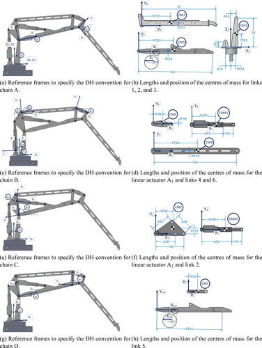
Table 3. DH parameters for homogeneous transformations of the open kinematic chains.

(a)
DH Parameters – Chain A
Ai	θi	${\mathrm{d}}_{\mathrm{i}}$	${\mathrm{a}}_{\mathrm{i}}$	αi
1	$q_1$	0	0	0
2	0	D3	A1A	$\pi /2$
3	$q_2$	0	0	0
4	$-{\alpha }_{10}$	0	A3	0
5	$-q_3$	0	0	0
(b)
DH Parameters – Chain B
Bi	θi	${\mathrm{d}}_{\mathrm{i}}$	${\mathrm{a}}_{\mathrm{i}}$	αi
1	$q_1$	D2	-A1B	$\pi /2$
2	$q_4$	0	0	0
3	0	0	AP1	0
4	$-\pi /2$	0	0	$-\pi /2$
5	0	$X1$	0	0
6	0	0	0	$\pi /2$
7	$\pi /2$	0	0	0
8	$-q_5$	0	A2B	0
9	$-q_6$	0	0	0
10	0	0	A4	0
11	$-q_7$	0	0	0
(c)
DH Parameters – Chain C
Ci	θi	${\mathrm{d}}_{\mathrm{i}}$	${\mathrm{a}}_{\mathrm{i}}$	αi
1	$q_1$	D3	A1A	$\pi /2$
2	$q_9$	0	0	0
3	0	0	A2D	0
4	$q_{10}$	0	0	0
(d)
DH Parameters – Chain D
Di	θi	${\mathrm{d}}_{\mathrm{i}}$	${\mathrm{a}}_{\mathrm{i}}$	αi
1	$q_1$	D3	A1A	$\pi /2$
2	$q_2$	0	A31X	0
3	$q_{11}$	0	0	0

Eq. (13)(13) $$\begin{array}{c}{\mathrm{T}}_{\text{CM}1}^0={\mathrm{A}}_1^0\left(\begin{array}{cccc}1& 0& 0& \text{PCX}1\\ 0& 1& 0& 0\\ 0& 0& 1& \text{PCZ}1\\ 0& 0& 0& 1\end{array}\right),\\ {\mathrm{T}}_{\text{CM}3}^0={\mathrm{A}}_2^0\left(\begin{array}{cccc}1& 0& 0& \text{PCX}3\\ 0& 1& 0& \text{PCY}3\\ 0& 0& 1& 0\\ 0& 0& 0& 1\end{array}\right),\\ {\mathrm{T}}_{\text{CM}7}^0={\mathrm{A}}_3^0\left(\begin{array}{cccc}1& 0& 0& \text{PCX}7\\ 0& 1& 0& \text{PCY}7\\ 0& 0& 1& 0\\ 0& 0& 0& 1\end{array}\right).\end{array}$$(13) shows the analytical expressions representing the position and orientation of CM1, CM3 and CM7, where ${\mathrm{A}}_1^0={\mathrm{A}}_1^0,{\mathrm{A}}_2^0={\mathrm{A}}_1^0{\mathrm{A}}_2^1{\mathrm{A}}_3^2$ and ${\mathrm{A}}_3^0={\mathrm{A}}_1^0{\mathrm{A}}_2^1{\mathrm{A}}_3^2{\mathrm{A}}_4^3{\mathrm{A}}_5^4.$ (13) $$\begin{array}{c}{\mathrm{T}}_{\text{CM}1}^0={\mathrm{A}}_1^0\left(\begin{array}{cccc}1& 0& 0& \text{PCX}1\\ 0& 1& 0& 0\\ 0& 0& 1& \text{PCZ}1\\ 0& 0& 0& 1\end{array}\right),\\ {\mathrm{T}}_{\text{CM}3}^0={\mathrm{A}}_2^0\left(\begin{array}{cccc}1& 0& 0& \text{PCX}3\\ 0& 1& 0& \text{PCY}3\\ 0& 0& 1& 0\\ 0& 0& 0& 1\end{array}\right),\\ {\mathrm{T}}_{\text{CM}7}^0={\mathrm{A}}_3^0\left(\begin{array}{cccc}1& 0& 0& \text{PCX}7\\ 0& 1& 0& \text{PCY}7\\ 0& 0& 1& 0\\ 0& 0& 0& 1\end{array}\right).\end{array}$$(13)

Chain B

For purposes of forward kinematics, it is convenient to join chains B1 and B2. The union of these chains is defined as chain B and its DH parameters are shown in Table 3(b). Reference frames and lengths to identify centers of mass position of the linear actuator ${\mathrm{A}}_1$ (CMA1), the link 4 (CM4) and the link 6 (CM6) are shown in Fig. 11 c and 11 d.

Eq. (14)(14) $$\begin{array}{c}{\mathrm{T}}_{\text{CMA}1}^0={\mathrm{B}}_2^0\left(\begin{array}{cccc}1& 0& 0& \text{PCXP}1+{\mathrm{K}}_{\mathrm{m}}X1\\ 0& 1& 0& 0\\ 0& 0& 1& 0\\ 0& 0& 0& 1\end{array}\right),\\ {\mathrm{T}}_{\text{CM}4}^0={\mathrm{B}}_9^0\left(\begin{array}{cccc}1& 0& 0& \text{PCX}4\\ 0& 1& 0& \text{PCY}4\\ 0& 0& 1& 0\\ 0& 0& 0& 1\end{array}\right),\\ {\mathrm{T}}_{\text{CM}6}^0={\mathrm{B}}_{11}^0\left(\begin{array}{cccc}1& 0& 0& \text{PCX}6\\ 0& 1& 0& \text{PCY}6\\ 0& 0& 1& 0\\ 0& 0& 0& 1\end{array}\right).\end{array}$$(14) shows the analytical expressions representing the position and orientation of CMA1, CM4 and CM6, where ${\mathrm{B}}_2^0={\mathrm{B}}_1^0{\mathrm{B}}_2^1,{\mathrm{B}}_9^0={\mathrm{B}}_1^0{\mathrm{B}}_2^1\dots {\mathrm{B}}_9^8,{\mathrm{B}}_{11}^0={\mathrm{B}}_1^0{\mathrm{B}}_2^1{\mathrm{B}}_3^2\dots {\mathrm{B}}_{11}^{10}$ and ${\mathrm{K}}_{\mathrm{m}}$ is a constant proportional to the displacement $X1.$ (14) $$\begin{array}{c}{\mathrm{T}}_{\text{CMA}1}^0={\mathrm{B}}_2^0\left(\begin{array}{cccc}1& 0& 0& \text{PCXP}1+{\mathrm{K}}_{\mathrm{m}}X1\\ 0& 1& 0& 0\\ 0& 0& 1& 0\\ 0& 0& 0& 1\end{array}\right),\\ {\mathrm{T}}_{\text{CM}4}^0={\mathrm{B}}_9^0\left(\begin{array}{cccc}1& 0& 0& \text{PCX}4\\ 0& 1& 0& \text{PCY}4\\ 0& 0& 1& 0\\ 0& 0& 0& 1\end{array}\right),\\ {\mathrm{T}}_{\text{CM}6}^0={\mathrm{B}}_{11}^0\left(\begin{array}{cccc}1& 0& 0& \text{PCX}6\\ 0& 1& 0& \text{PCY}6\\ 0& 0& 1& 0\\ 0& 0& 0& 1\end{array}\right).\end{array}$$(14)

Chain C and chain D

Table 3(c) and 3(d) show the DH parameters for chain C and chain D, respectively, while Figs. 11(e)–11(h) show reference frames and lengths to identify the centers of mass position of the linear actuator ${\mathrm{A}}_2$ (CMA2), the link 2 (CM2) and the link 5 (CM5).

Finally, Eq. (15)(15) $$\begin{array}{c}{\mathrm{T}}_{\text{CM}2}^0={\mathrm{C}}_2^0\left(\begin{array}{cccc}1& 0& 0& \text{PCX}2\\ 0& 1& 0& \text{PCY}2\\ 0& 0& 1& 0\\ 0& 0& 0& 1\end{array}\right),\\ {\mathrm{T}}_{\text{CMA}2}^0={\mathrm{C}}_4^0\left(\begin{array}{cccc}1& 0& 0& \text{PCXP}2+{\mathrm{K}}_{\mathrm{m}}X2\\ 0& 1& 0& 0\\ 0& 0& 1& 0\\ 0& 0& 0& 1\end{array}\right),\\ {\mathrm{T}}_{\text{CM}5}^0={\mathrm{D}}_3^0\left(\begin{array}{cccc}1& 0& 0& \text{PCX}5\\ 0& 1& 0& \text{PCY}5\\ 0& 0& 1& 0\\ 0& 0& 0& 1\end{array}\right).\end{array}$$(15) shows the analytical expressions representing position and orientation of CM2, CMA2 and CM5, where ${\mathrm{C}}_2^0={\mathrm{C}}_1^0{\mathrm{C}}_2^1,{\mathrm{C}}_4^0={\mathrm{C}}_1^0{\mathrm{C}}_2^1{\mathrm{C}}_3^2{\mathrm{C}}_4^3,{\mathrm{D}}_3^0={\mathrm{D}}_1^0{\mathrm{D}}_2^1{\mathrm{D}}_3^2$ and ${\mathrm{K}}_{\mathrm{m}}$ is a constant proportional to the displacement $X2.$ (15) $$\begin{array}{c}{\mathrm{T}}_{\text{CM}2}^0={\mathrm{C}}_2^0\left(\begin{array}{cccc}1& 0& 0& \text{PCX}2\\ 0& 1& 0& \text{PCY}2\\ 0& 0& 1& 0\\ 0& 0& 0& 1\end{array}\right),\\ {\mathrm{T}}_{\text{CMA}2}^0={\mathrm{C}}_4^0\left(\begin{array}{cccc}1& 0& 0& \text{PCXP}2+{\mathrm{K}}_{\mathrm{m}}X2\\ 0& 1& 0& 0\\ 0& 0& 1& 0\\ 0& 0& 0& 1\end{array}\right),\\ {\mathrm{T}}_{\text{CM}5}^0={\mathrm{D}}_3^0\left(\begin{array}{cccc}1& 0& 0& \text{PCX}5\\ 0& 1& 0& \text{PCY}5\\ 0& 0& 1& 0\\ 0& 0& 0& 1\end{array}\right).\end{array}$$(15)

B dynamic modelling of the open kinematic chains

Dynamic model of chain A

Chain A considers three links connected via three rotational joints, so the vector of generalized coordinates is defined as ${\mathrm{q}}_{\mathrm{a}}={[q_1,q_2,q_3]}^{\mathrm{T}}.$ The dynamic model of chain A considering the homogeneous transformations in Eq. (2.2(2) $$\begin{array}{c}{\mathbf{D}}_{\mathbf{PA}}({\mathbf{q}}_{\mathbf{PA}})\stackrel{..}{{\mathbf{q}}_{\mathbf{PA}}}\mathit{+}{\mathbf{C}}_{\mathbf{PA}}({\mathbf{q}}_{\mathbf{PA}},\stackrel{.}{{\mathbf{q}}_{\mathbf{PA}}})\stackrel{.}{{\mathbf{q}}_{\mathbf{PA}}}\hfill \\ \mathit{+}{\mathbf{G}}_{\mathbf{PA}}({\mathbf{q}}_{\mathbf{PA}})\mathit{=}{\mathit{\tau }}_{\mathbf{PA}},\hfill \\ {\mathbf{q}}_{\mathbf{PA}}=\begin{array}{c}\left(\begin{array}{c}{q}_1\\ q_2\\ q_3\\ q_4\\ X1\\ q_6\\ q_7\\ q_9\\ q_{10}\\ X2\\ q_{11}\end{array}\right)\hfill \end{array};{\mathit{\tau }}_{\mathbf{PA}}=\begin{array}{c}\left(\begin{array}{c}{\tau }_1\\ {\tau }_2\\ {\tau }_3\\ {\tau }_4\\ F_{A1}\\ {\tau }_6\\ {\tau }_7\\ {\tau }_9\\ {\tau }_{10}\\ F_{A2}\\ {\tau }_{11}\end{array}\right)\hfill \end{array}.\hfill \end{array}$$(2) .2) is stated as, (16) $${\mathrm{D}}_{\mathrm{a}}({\mathrm{q}}_{\mathrm{a}})\stackrel{..}{{\mathrm{q}}_{\mathrm{a}}}+{\mathrm{C}}_{\mathrm{a}}({\mathrm{q}}_{\mathrm{a}},\stackrel{.}{{\mathrm{q}}_{\mathrm{a}}})\stackrel{.}{{\mathrm{q}}_{\mathrm{a}}}+{\mathrm{G}}_{\mathrm{a}}({\mathrm{q}}_{\mathrm{a}})={\tau }_a.$$(16)

Dynamic model of chain B1

Chain B1 is formed only by the linear actuator A1, however, the vector of generalized coordinates has one rotational joint and one prismatic joint, and it is defined as ${\mathrm{q}}_{\mathrm{b}1}={[q_4,X1]}^{\mathrm{T}}.$ The dynamic model of chain B1 considering the homogeneous transformation ${\mathrm{T}}_{\text{CMA}1}^0$ in Eq. (14)(14) $$\begin{array}{c}{\mathrm{T}}_{\text{CMA}1}^0={\mathrm{B}}_2^0\left(\begin{array}{cccc}1& 0& 0& \text{PCXP}1+{\mathrm{K}}_{\mathrm{m}}X1\\ 0& 1& 0& 0\\ 0& 0& 1& 0\\ 0& 0& 0& 1\end{array}\right),\\ {\mathrm{T}}_{\text{CM}4}^0={\mathrm{B}}_9^0\left(\begin{array}{cccc}1& 0& 0& \text{PCX}4\\ 0& 1& 0& \text{PCY}4\\ 0& 0& 1& 0\\ 0& 0& 0& 1\end{array}\right),\\ {\mathrm{T}}_{\text{CM}6}^0={\mathrm{B}}_{11}^0\left(\begin{array}{cccc}1& 0& 0& \text{PCX}6\\ 0& 1& 0& \text{PCY}6\\ 0& 0& 1& 0\\ 0& 0& 0& 1\end{array}\right).\end{array}$$(14) is stated as, (17) $${\mathrm{D}}_{\mathrm{b}1}({\mathrm{q}}_{\mathrm{b}1})\stackrel{..}{{\mathrm{q}}_{\mathrm{b}1}}+{\mathrm{C}}_{\mathrm{b}1}({\mathrm{q}}_{\mathrm{b}1},\stackrel{.}{{\mathrm{q}}_{\mathrm{b}1}})\stackrel{.}{{\mathrm{q}}_{\mathrm{b}1}}+{\mathrm{G}}_{\mathrm{b}1}({\mathrm{q}}_{\mathrm{b}1})={\tau }_{b1}.$$(17)

Dynamic model of chain B2

Chain B2 is formed by two links with two rotational joints, so the vector of generalized coordinates is defined as ${\mathrm{q}}_{\mathrm{b}2}={[q_6,q_7]}^{\mathrm{T}}.$ The dynamic model of chain B2 considering the homogeneous transformations ${\mathrm{T}}_{\text{CM}4}^0$ and ${\mathrm{T}}_{\text{CM}6}^0$ in Eq. (14)(14) $$\begin{array}{c}{\mathrm{T}}_{\text{CMA}1}^0={\mathrm{B}}_2^0\left(\begin{array}{cccc}1& 0& 0& \text{PCXP}1+{\mathrm{K}}_{\mathrm{m}}X1\\ 0& 1& 0& 0\\ 0& 0& 1& 0\\ 0& 0& 0& 1\end{array}\right),\\ {\mathrm{T}}_{\text{CM}4}^0={\mathrm{B}}_9^0\left(\begin{array}{cccc}1& 0& 0& \text{PCX}4\\ 0& 1& 0& \text{PCY}4\\ 0& 0& 1& 0\\ 0& 0& 0& 1\end{array}\right),\\ {\mathrm{T}}_{\text{CM}6}^0={\mathrm{B}}_{11}^0\left(\begin{array}{cccc}1& 0& 0& \text{PCX}6\\ 0& 1& 0& \text{PCY}6\\ 0& 0& 1& 0\\ 0& 0& 0& 1\end{array}\right).\end{array}$$(14) is stated as, (18) $${\mathrm{D}}_{\mathrm{b}2}({\mathrm{q}}_{\mathrm{b}2})\stackrel{..}{{\mathrm{q}}_{\mathrm{b}2}}+{\mathrm{C}}_{\mathrm{b}2}({\mathrm{q}}_{\mathrm{b}2},\stackrel{.}{{\mathrm{q}}_{\mathrm{b}2}})\stackrel{.}{{\mathrm{q}}_{\mathrm{b}2}}+{\mathrm{G}}_{\mathrm{b}2}({\mathrm{q}}_{\mathrm{b}2})={\tau }_{b2}.$$(18)

Dynamic model of chain C

Chain C considers two elements, and the vector of generalized coordinates for this chain is defined as ${\mathrm{q}}_{\mathrm{c}}={[q_9,q_{10},X2]}^{\mathrm{T}}.$ The dynamic model of chain C considering the homogeneous transformations ${\mathrm{T}}_{\text{CM}2}^0$ and ${\mathrm{T}}_{\text{CMA}2}^0$ in Eq. (15)(15) $$\begin{array}{c}{\mathrm{T}}_{\text{CM}2}^0={\mathrm{C}}_2^0\left(\begin{array}{cccc}1& 0& 0& \text{PCX}2\\ 0& 1& 0& \text{PCY}2\\ 0& 0& 1& 0\\ 0& 0& 0& 1\end{array}\right),\\ {\mathrm{T}}_{\text{CMA}2}^0={\mathrm{C}}_4^0\left(\begin{array}{cccc}1& 0& 0& \text{PCXP}2+{\mathrm{K}}_{\mathrm{m}}X2\\ 0& 1& 0& 0\\ 0& 0& 1& 0\\ 0& 0& 0& 1\end{array}\right),\\ {\mathrm{T}}_{\text{CM}5}^0={\mathrm{D}}_3^0\left(\begin{array}{cccc}1& 0& 0& \text{PCX}5\\ 0& 1& 0& \text{PCY}5\\ 0& 0& 1& 0\\ 0& 0& 0& 1\end{array}\right).\end{array}$$(15) is stated as, (19) $${\mathrm{D}}_{\mathrm{c}}({\mathrm{q}}_{\mathrm{c}})\stackrel{..}{{\mathrm{q}}_{\mathrm{c}}}+{\mathrm{C}}_{\mathrm{c}}({\mathrm{q}}_{\mathrm{c}},\stackrel{.}{{\mathrm{q}}_{\mathrm{c}}})\stackrel{.}{{\mathrm{q}}_{\mathrm{c}}}+{\mathrm{G}}_{\mathrm{c}}({\mathrm{q}}_{\mathrm{c}})={\tau }_c.$$(19)

Dynamic model of chain D

Chain D considers only link 5, so the vector of generalized coordinates is defined as ${\mathrm{q}}_{\mathrm{d}}=q_{11}.$ Finally, the dynamic model of chain D considering the homogeneous transformation ${\mathrm{T}}_{\text{CM}5}^0$ in Eq. (15)(15) $$\begin{array}{c}{\mathrm{T}}_{\text{CM}2}^0={\mathrm{C}}_2^0\left(\begin{array}{cccc}1& 0& 0& \text{PCX}2\\ 0& 1& 0& \text{PCY}2\\ 0& 0& 1& 0\\ 0& 0& 0& 1\end{array}\right),\\ {\mathrm{T}}_{\text{CMA}2}^0={\mathrm{C}}_4^0\left(\begin{array}{cccc}1& 0& 0& \text{PCXP}2+{\mathrm{K}}_{\mathrm{m}}X2\\ 0& 1& 0& 0\\ 0& 0& 1& 0\\ 0& 0& 0& 1\end{array}\right),\\ {\mathrm{T}}_{\text{CM}5}^0={\mathrm{D}}_3^0\left(\begin{array}{cccc}1& 0& 0& \text{PCX}5\\ 0& 1& 0& \text{PCY}5\\ 0& 0& 1& 0\\ 0& 0& 0& 1\end{array}\right).\end{array}$$(15) is stated as, (20) $${\mathrm{D}}_{\mathrm{d}}({\mathrm{q}}_{\mathrm{d}})\stackrel{..}{{\mathrm{q}}_{\mathrm{d}}}+{\mathrm{C}}_{\mathrm{d}}({\mathrm{q}}_{\mathrm{d}},\stackrel{.}{{\mathrm{q}}_{\mathrm{d}}})\stackrel{.}{{\mathrm{q}}_{\mathrm{d}}}+{\mathrm{G}}_{\mathrm{d}}({\mathrm{q}}_{\mathrm{d}})={\tau }_d.$$(20)

Finally, Eq. (21)(21) $$\begin{array}{cc}\begin{array}{c}\left(\begin{array}{ccccc}{\mathrm{D}}_{\mathrm{a}}& 0_{3\times 2}& 0_{3\times 2}& 0_{3\times 3}& 0_{3\times 1}\\ 0_{2\times 3}& {\mathrm{D}}_{\mathrm{b}1}& 0_{2\times 2}& 0_{2\times 3}& 0_{2\times 1}\\ 0_{2\times 3}& 0_{2\times 2}& {\mathrm{D}}_{\mathrm{b}2}& 0_{2\times 3}& 0_{2\times 1}\\ 0_{3\times 3}& 0_{3\times 2}& 0_{3\times 2}& {\mathrm{D}}_{\mathrm{c}}& 0_{3\times 1}\\ 0_{1\times 3}& 0_{1\times 2}& 0_{1\times 2}& 0_{1\times 3}& {\mathrm{D}}_{\mathrm{d}}\end{array}\right)\left(\begin{array}{c}\stackrel{..}{{\mathrm{q}}_{\mathrm{a}}}\\ \stackrel{..}{{\mathrm{q}}_{\mathrm{b}1}}\\ \stackrel{..}{{\mathrm{q}}_{\mathrm{b}2}}\\ \stackrel{..}{{\mathrm{q}}_{\mathrm{c}}}\\ \stackrel{..}{{\mathrm{q}}_{\mathrm{d}}}\end{array}\right)\hfill \end{array}\hfill & +\hfill \\ \begin{array}{c}\left(\begin{array}{ccccc}{\mathrm{C}}_{\mathrm{a}}& 0_{3\times 2}& 0_{3\times 2}& 0_{3\times 3}& 0_{3\times 1}\\ 0_{2\times 3}& {\mathrm{C}}_{\mathrm{b}1}& 0_{2\times 2}& 0_{2\times 3}& 0_{2\times 1}\\ 0_{2\times 3}& 0_{2\times 2}& {\mathrm{C}}_{\mathrm{b}2}& 0_{2\times 3}& 0_{2\times 1}\\ 0_{3\times 3}& 0_{3\times 2}& 0_{3\times 2}& {\mathrm{C}}_{\mathrm{c}}& 0_{3\times 1}\\ 0_{1\times 3}& 0_{1\times 2}& 0_{1\times 2}& 0_{1\times 3}& {\mathrm{C}}_{\mathrm{d}}\end{array}\right)\left(\begin{array}{c}\stackrel{.}{{\mathrm{q}}_{\mathrm{a}}}\\ \stackrel{.}{{\mathrm{q}}_{\mathrm{b}1}}\\ \stackrel{.}{{\mathrm{q}}_{\mathrm{b}2}}\\ \stackrel{.}{{\mathrm{q}}_{\mathrm{c}}}\\ \stackrel{.}{{\mathrm{q}}_{\mathrm{d}}}\end{array}\right)\hfill \end{array}\hfill & +\begin{array}{c}\left(\begin{array}{c}{\mathrm{G}}_{\mathrm{a}}\\ {\mathrm{G}}_{\mathrm{b}1}\\ {\mathrm{G}}_{\mathrm{b}2}\\ {\mathrm{G}}_{\mathrm{c}}\\ {\mathrm{G}}_{\mathrm{d}}\end{array}\right)\hfill \end{array}\hfill \\ =\begin{array}{c}\left(\begin{array}{c}{\tau }_{\mathrm{a}}\\ {\tau }_{\mathrm{b}1}\\ {\tau }_{\mathrm{b}2}\\ {\tau }_{\mathrm{c}}\\ {\tau }_{\mathrm{d}}\end{array}\right)\hfill \end{array}.\hfill & \hfill \end{array}$$(21) states the dynamic model when considering all the open kinematic chains without kinematic constraints. (21) $$\begin{array}{cc}\begin{array}{c}\left(\begin{array}{ccccc}{\mathrm{D}}_{\mathrm{a}}& 0_{3\times 2}& 0_{3\times 2}& 0_{3\times 3}& 0_{3\times 1}\\ 0_{2\times 3}& {\mathrm{D}}_{\mathrm{b}1}& 0_{2\times 2}& 0_{2\times 3}& 0_{2\times 1}\\ 0_{2\times 3}& 0_{2\times 2}& {\mathrm{D}}_{\mathrm{b}2}& 0_{2\times 3}& 0_{2\times 1}\\ 0_{3\times 3}& 0_{3\times 2}& 0_{3\times 2}& {\mathrm{D}}_{\mathrm{c}}& 0_{3\times 1}\\ 0_{1\times 3}& 0_{1\times 2}& 0_{1\times 2}& 0_{1\times 3}& {\mathrm{D}}_{\mathrm{d}}\end{array}\right)\left(\begin{array}{c}\stackrel{..}{{\mathrm{q}}_{\mathrm{a}}}\\ \stackrel{..}{{\mathrm{q}}_{\mathrm{b}1}}\\ \stackrel{..}{{\mathrm{q}}_{\mathrm{b}2}}\\ \stackrel{..}{{\mathrm{q}}_{\mathrm{c}}}\\ \stackrel{..}{{\mathrm{q}}_{\mathrm{d}}}\end{array}\right)\hfill \end{array}\hfill & +\hfill \\ \begin{array}{c}\left(\begin{array}{ccccc}{\mathrm{C}}_{\mathrm{a}}& 0_{3\times 2}& 0_{3\times 2}& 0_{3\times 3}& 0_{3\times 1}\\ 0_{2\times 3}& {\mathrm{C}}_{\mathrm{b}1}& 0_{2\times 2}& 0_{2\times 3}& 0_{2\times 1}\\ 0_{2\times 3}& 0_{2\times 2}& {\mathrm{C}}_{\mathrm{b}2}& 0_{2\times 3}& 0_{2\times 1}\\ 0_{3\times 3}& 0_{3\times 2}& 0_{3\times 2}& {\mathrm{C}}_{\mathrm{c}}& 0_{3\times 1}\\ 0_{1\times 3}& 0_{1\times 2}& 0_{1\times 2}& 0_{1\times 3}& {\mathrm{C}}_{\mathrm{d}}\end{array}\right)\left(\begin{array}{c}\stackrel{.}{{\mathrm{q}}_{\mathrm{a}}}\\ \stackrel{.}{{\mathrm{q}}_{\mathrm{b}1}}\\ \stackrel{.}{{\mathrm{q}}_{\mathrm{b}2}}\\ \stackrel{.}{{\mathrm{q}}_{\mathrm{c}}}\\ \stackrel{.}{{\mathrm{q}}_{\mathrm{d}}}\end{array}\right)\hfill \end{array}\hfill & +\begin{array}{c}\left(\begin{array}{c}{\mathrm{G}}_{\mathrm{a}}\\ {\mathrm{G}}_{\mathrm{b}1}\\ {\mathrm{G}}_{\mathrm{b}2}\\ {\mathrm{G}}_{\mathrm{c}}\\ {\mathrm{G}}_{\mathrm{d}}\end{array}\right)\hfill \end{array}\hfill \\ =\begin{array}{c}\left(\begin{array}{c}{\tau }_{\mathrm{a}}\\ {\tau }_{\mathrm{b}1}\\ {\tau }_{\mathrm{b}2}\\ {\tau }_{\mathrm{c}}\\ {\tau }_{\mathrm{d}}\end{array}\right)\hfill \end{array}.\hfill & \hfill \end{array}$$(21)

C solution to the kinematic constraint ${\mathrm{f}}_{{\mathrm{q}}_4}$

Fig. 12 shows the schematic representation to solve ${\mathrm{f}}_{{\mathrm{q}}_4},$ where it can be seen that: (22) $$\begin{array}{ccc}{\mathrm{f}}_{{\mathrm{q}}_4}(X1,X2)& =& q_4(X1)\\ q_4(X1)& =& {\alpha }_2(X1)+{\alpha }_1\end{array}.$$(22)

Figure 12. Schematic representation for the solution to the kinematic constraint ${\mathrm{f}}_{{\mathrm{q}}_4}.$

By using trigonometric identities it can be stated that: (23) $${\alpha }_1={\hspace{0.17em}\text{tan}\hspace{0.17em}}^{-1}\left(\frac{\mathrm{D}3-\mathrm{D}2}{\mathrm{A}1\mathrm{A}+\mathrm{A}1\mathrm{B}}\right),$$(23) (24) $${\text{LR}4}^2={(\mathrm{D}3-\mathrm{D}2)}^2+{(\mathrm{A}1\mathrm{A}+\mathrm{A}1\mathrm{B})}^2.$$(24)

By using law of cosines, (25) $${\alpha }_2(X1)={\hspace{0.17em}\text{cos}\hspace{0.17em}}^{-1}\left(\frac{{\mathrm{A}2\mathrm{C}}^2-{(\text{AP}1+X1)}^2{-\text{LR}4}^2}{-2(\text{AP}1+X1)(\text{LR}4)}\right).$$(25)

Once ${\alpha }_1$ and ${\alpha }_2(X1)$ are known, it is possible to obtain $\mathit{\gamma }$ for ${\mathrm{f}}_{{\mathrm{q}}_4}(X1,X2).$ From Eq. (4)(4) $$\begin{array}{c}{\mathit{\gamma }}^{\mathit{T}}{\mathbf{D}}_{\mathbf{PA}}({\mathbf{q}}_{\mathbf{A}})\mathit{\gamma }\stackrel{..}{{\mathbf{q}}_{\mathbf{A}}}\mathit{+}\hfill \\ {\mathit{\gamma }}^{\mathit{T}}({\mathbf{D}}_{\mathbf{PA}}({\mathbf{q}}_{\mathbf{A}})\dot{\mathit{\gamma }}\mathit{+}{\mathbf{C}}_{\mathbf{PA}}({\mathbf{q}}_{\mathbf{A}},\stackrel{.}{{\mathbf{q}}_{\mathbf{A}}}))\stackrel{.}{{\mathbf{q}}_{\mathbf{A}}}\mathit{+}\hfill \\ {\mathit{\gamma }}^{\mathit{T}}{\mathbf{G}}_{\mathbf{PA}}({\mathbf{q}}_{\mathbf{A}})\mathit{=}{\mathit{\tau }}_{\mathbf{A}},\hfill \\ \mathit{\gamma }=\begin{array}{c}\left(\begin{array}{ccc}1& 0& 0\\ 0& \frac{\partial {\mathrm{f}}_{{\mathrm{q}}_2}(X1,X2)}{\partial X1}& \frac{\partial {\mathrm{f}}_{{\mathrm{q}}_2}(X1,X2)}{\partial X2}\\ 0& \frac{\partial {\mathrm{f}}_{{\mathrm{q}}_3}(X1,X2)}{\partial X1}& \frac{\partial {\mathrm{f}}_{{\mathrm{q}}_3}(X1,X2)}{\partial X2}\\ 0& \frac{\partial {\mathrm{f}}_{{\mathrm{q}}_4}(X1,X2)}{\partial X1}& \frac{\partial {\mathrm{f}}_{{\mathrm{q}}_4}(X1,X2)}{\partial X2}\\ 0& 1& 0\\ 0& \frac{\partial {\mathrm{f}}_{{\mathrm{q}}_6}(X1,X2)}{\partial X1}& \frac{\partial {\mathrm{f}}_{{\mathrm{q}}_6}(X1,X2)}{\partial X2}\\ 0& \frac{\partial {\mathrm{f}}_{{\mathrm{q}}_7}(X1,X2)}{\partial X1}& \frac{\partial {\mathrm{f}}_{{\mathrm{q}}_7}(X1,X2)}{\partial X2}\\ 0& \frac{\partial {\mathrm{f}}_{{\mathrm{q}}_9}(X1,X2)}{\partial X1}& \frac{\partial {\mathrm{f}}_{{\mathrm{q}}_9}(X1,X2)}{\partial X2}\\ 0& \frac{\partial {\mathrm{f}}_{{\mathrm{q}}_{10}}(X1,X2)}{\partial X1}& \frac{\partial {\mathrm{f}}_{{\mathrm{q}}_{10}}(X1,X2)}{\partial X2}\\ 0& 0& 1\\ 0& \frac{\partial {\mathrm{f}}_{{\mathrm{q}}_{11}}(X1,X2)}{\partial X1}& \frac{\partial {\mathrm{f}}_{{\mathrm{q}}_{11}}(X1,X2)}{\partial X2}\end{array}\right)\hfill \end{array}\hfill \end{array}.$$(4) , it can be seen that: (26) $${\mathit{\gamma }}_{{\mathrm{f}}_{{\mathrm{q}}_4}(X1,X2)}=\begin{array}{c}\left(\begin{array}{ccc}0& \frac{\partial {\mathrm{f}}_{{\mathrm{q}}_4}(X1,X2)}{\partial X1}& \frac{\partial {\mathrm{f}}_{{\mathrm{q}}_4}(X1,X2)}{\partial X2}\end{array}\right)\end{array},$$(26) where (27) $$\begin{array}{c}\frac{\partial {\mathrm{f}}_{{\mathrm{q}}_4}(X1,X2)}{\partial X1}=\frac{\partial {\alpha }_1}{\partial X1}+\frac{\partial {\alpha }_2(X1)}{\partial X1}\\ \frac{\partial {\mathrm{f}}_{{\mathrm{q}}_4}(X1,X2)}{\partial X2}=\frac{\partial {\alpha }_1}{\partial X2}+\frac{\partial {\alpha }_2(X1)}{\partial X2}\end{array}.$$(27)

Finally, it can be stated that: (28) $${\mathit{\gamma }}_{{\mathrm{f}}_{{\mathrm{q}}_4}(X1,X2)}=\begin{array}{c}\left(\begin{array}{ccc}0& \frac{\frac{-1}{LR4}+\frac{2({(AP1+X1)}^2-A2C^2+LR{4}^2)}{LR4{(2AP1+2X1)}^2}}{\sqrt{1-\frac{{({(AP1+X1)}^2-A2C^2+LR{4}^2)}^2}{LR{4}^2{(2AP1+2X1)}^2}}}& 0\end{array}\right)\end{array}.$$(28)

References

- Arnold, M. 2017. DAE aspects of multibody system dynamics. In Surveys in differential-algebraic equations IV, 41–206. Heidelberg: Springer International Publishing.
- Bin Ishak, I., D. Fleming, and P. Larochelle. 2019. Multiplane fused deposition modeling: A study of tensile strength. Mechanics Based Design of Structures and Machines 47 (5):5:583–598. doi:10.1080/15397734.2019.1596127.
- Bin Ishak, I., and P. Larochelle. 2019. Motomaker: A robot fdm platform for multi-plane and 3d lattice structure printing. Mechanics Based Design of Structures and Machines 47 (6):703–20. doi:10.1080/15397734.2019.1615943.
- Brennan, S., and A. Alleyne. 2001. Using a scale testbed: Controller design and evaluation. IEEE Control Systems Magazine 21:15–26.
- Eckert, J., F. Mazzariol, E. Bertoti, E. Dos Santos Costa, F. Corrêa, C. de Alkmin, and F. Giuseppe. 2018. Gear shifting multi-objective optimization to improve vehicle performance, fuel consumption, and engine emissions. Mechanics Based Design of Structures and Machines 46 (2):238–53. doi:10.1080/15397734.2017.1330156.
- Esteban, E., O. Salgado, A. Iturrospe, and I. Isasa. 2017. Design methodology of a reduced-scale test bench for fault detection and diagnosis. Mechatronics 47:14–23. doi:10.1016/j.mechatronics.2017.08.005.
- Favrel, A., J. Pereira Junior, C. Landry, A. M, K. Yamaishi, and F. Avellan. 2019. Dynamic modal analysis during reduced scale model tests of hydraulic turbines for hydro-acoustic characterization of cavitation flows. Mechanical Systems and Signal Processing 117:81–96. doi:10.1016/j.ymssp.2018.07.053.
- Gaz, C., E. Magrini, and A. De Luca. 2018. A model-based residual approach for human-robot collaboration during manual polishing operations. Mechatronics 55:234–47. doi:10.1016/j.mechatronics.2018.02.014.
- Glocker, C. 2013. Set-valued force laws: Dynamics of non-smooth systems. Berlin: Springer Science & Business Media.
- Häggström, C., and O. Lindroos. 2016. Human, technology, organization and environment – A human factors perspective on performance in forest harvesting. International Journal of Forest Engineering 27:67–78.
- Hassan, A., and M. Abomoharam. 2017. Modeling and design optimization of a robot gripper mechanism. Robotics and Computer-Integrated Manufacturing 46:94–103. doi:10.1016/j.rcim.2016.12.012.
- Kalmari, J., J. Backman, and A. Visala. 2017. Coordinated motion of a hydraulic forestry crane and a vehicle using nonlinear model predictive control. Computers and Electronics in Agriculture 133:119–27. doi:10.1016/j.compag.2016.12.013.
- Koivumäki, J., and J. Mattila. 2015. Stability-guaranteed force-sensorless contact force/motion control of heavy-duty hydraulic manipulators. IEEE Transactions on Robotics 31 (4):918–35. doi:10.1109/TRO.2015.2441492.
- La Hera, P., and D. Ortiz Morales. 2014. Non-linear dynamics modeling description for simulating the behaviour of forestry cranes. International Journal of Modelling, Identification and Control 21 (2):125–37. doi:10.1504/IJMIC.2014.060006.
- La Hera, P., and D. Ortiz Morales. 2019. What do we observe when we equip a forestry crane with motion sensors? Croatian Journal of Forest Engineering 40 (2):259–80. doi:10.5552/crojfe.2019.501.
- Li, X., G. Wang, S. Miao, and X. Li. 2017. Optimal design of a hydraulic excavator working device based on parallel particle swarm optimization. Journal of the Brazilian Society of Mechanical Sciences and Engineering 39 (10):3793–805. doi:10.1007/s40430-017-0798-5.
- Ljung, L. 1999. System identification: Theory for the user. NJ: Prentice Hall PTR.
- Manner, J., A. Mörk, and M. Englund. 2019. Comparing forwarder boom-control systems based on an automatically recorded follow-up dataset. Silva Fennica 53 (2):10161. doi:10.14214/sf.10161.
- Mattila, J., J. Koivumäki, D. Caldwell, and C. Semini. 2017. A survey on control of hydraulic robotic manipulators with projection to future trends. IEEE/ASME Transactions on Mechatronics 22 (2):669–80. doi:10.1109/TMECH.2017.2668604.
- Mendoza-Trejo, O., and C. Cruz-Villar. 2016. Modelling and experimental validation of a planar 2-dof cobot as a differential-algebraic equation system. Applied Mathematical Modelling 40 (21-22):9327–41. doi:10.1016/j.apm.2016.06.007.
- Mick, S., M. Lapeyre, P. Rouanet, C. Halgand, J. Benois-Pineau, F. Paclet, D. Cattaert, P. Oudeyer, and A. Rugy. 2019. Reachy, a 3d-printed human-like robotic arm as a testbed for human-robot control strategies. Frontier in Neurorobotics 13 (65). doi:10.3389/fnbot.2019.00065.
- Mitrev, R., D. Janosević, and D. Marinković. 2017. Dynamical moodeling of hydraulic excavator considered as a multibody system. Technical Gazzete 24 (2):327–38.
- Mitrev, R., and D. Marinković. 2019. Numerical study of the hydraulic excavator overturning stability during performing lifting operations. Advances in Mechanical Engineering 11 (5):168781401984177–14. doi:10.1177/1687814019841779.
- Morales, D. O., P. L. Hera, S. Westerberg, L. B. Freidovich, and A. S. Shiriaev. 2015. Path-constrained motion analysis: An algorithm to understand human performance on hydraulic manipulators. IEEE Transactions on Human-Machine Systems 45 (2):187–99. doi:10.1109/THMS.2014.2366873.
- Nordfjell, T., E. Öhman, O. Lindroos, and B. Ager. 2019. The technical development of forwarders in modeli between 1962 and 2012 and of sales between 1975 and 2017. International Journal of Forest Engineering 30 (1):1–13. doi:10.1080/14942119.2019.1591074.
- Olsson, H., K. J. Åström, C. C. De Wit, M. Gäfvert, and P. Lischinsky. 1998. Friction models and friction compensation. European Journal of Control 4 (3):176–95. doi:10.1016/S0947-3580(98)70113-X.
- Ortiz Morales, D., S. Westerberg, P. X. La Hera, U. Mettin, L. Freidovich, and A. S. Shiriaev. 2014. Increasing the level of automation in the forestry logging process with crane trajectory planning and control. Journal of Field Robotics 31 (3):343–63. doi:10.1002/rob.21496.
- Park, F., J. Choi, and S. Ploen. 1999. Symbolic formulation of closed chain dynamics in independent coordinates. Mechanism and Machine Theory 34 (5):731–51. doi:10.1016/S0094-114X(98)00052-4.
- Salinić, S., G. Bosković, and M. Nikolić. 2014. Dynamic modeling of hydraulic excavator motion using Kane’s equations. Automation in Construction 44:56–62. doi:10.1016/j.autcon.2014.03.024.
- Siciliano, B. L. Sciavicco, L. Villani, and G. Oriolo. 2010. Robotics modeling, planning and control. NJ: Springer-Verlag.
- Spong, M. S. Hutchinson, and M. Vidyasagar. 2006. Robotics modeling and control. NY: John Wiley & Sons, Inc.
- Vallés, M., P. Araujo-Gómez, V. Mata, A. Valera, M. Díaz-Rodríguez, A. Page, and M. Farhat. 2018. Mechatronic design, experimental setup, and control architecture design of a novel 4 dof parallel manipulator. Mechanics Based Design of Structures and Machines 46 (4):425–39. doi:10.1080/15397734.2017.1355249.
- Vihonen, J., J. Mattila, and A. Visa. 2017. Joint-space kinematic model for gravity-referenced joint angle estimation of heavy-duty manipulators. IEEE Transactions on Instrumentation and Measurement 66 (12):3280–8. doi:10.1109/TIM.2017.2749918.
- Xu, G., H. Ding, and Z. Feng. 2019. Optimal design of hydraulic excavator shovel attachment based on multiobjective evolutionary algorithm. IEEE/ASME Transactions on Mechatronics 24 (2):808–19. doi:10.1109/TMECH.2019.2903140.