Trade Liberalization and Manufacturing Productivity in Nepal: Examining a Small Open Developing Economy

ABSTRACT

This study examines the trade-productivity nexus using manufacturing industry data during Nepal’s rapid trade reform period that intensified from the early 1990s. Productivity improvements from trade liberalization only accrue to large industries and the highly efficient industries along the productivity quantiles. Methodologically, the results indicate that one should examine distributional variations as well as conditional mean variations to capture all relevant industry productivity responses to trade policy changes. These results imply that there is ample opportunity for Nepal to continue reaping benefits from the trade liberalization process as more industries grow in size and become more efficient over time.

KEYWORDS:

• Trade liberalization
• Nepal
• productivity quantiles
• manufacturing sector
• industry characteristics

JEL:

• C23
• D24
• F13
• F14
• O53

1. Introduction

Trade is considered an important engine of economic growth, especially for small, open developing economies. The general view is that cross-border flows of goods and services bring about new economic opportunities to a country. Over the past three decades, trade liberalization has therefore become a major part of countries’ development strategies. For a more outward-oriented economy, as defined by Santos‐Paulino (2005), trade liberalization leads to more efficient resource allocations through foreign competition and foreign direct investment, resulting in productivity improvement for domestic industries (Topalova and Khandelwal 2011). On the other hand, critics argue that trade liberalization introduces external shocks to an economy, which leads to greater risks and uncertainty that adversely affect domestic industries and workers. This paper investigates the trade-productivity nexus in Nepal following the country’s economic liberalization that commenced in the mid-1980s and then accelerated in 1992. While several studies examine average productivity responses to lower trade protection through liberalization policies, scant empirical evidence, however, exists on distributional productivity responses.¹ Hence, the present study investigates whether trade liberalization is uniformly beneficial to all manufacturing industries in Nepal.

Nepal started adopting economic reform measures in the mid-1980s under the condition of the Structural Adjustment Program (SAP) in cooperation with the International Monetary Fund (IMF) and the World Bank (WTO 2012). This reform process was further intensified in 1992 when Nepal’s new democratically elected government implemented a series of market-oriented policy reforms, which aimed to accelerate opening up the domestic economy to lift economic growth (Biggs et al. 2000). Reforms included the full convertibility of the rupee, elimination of quantitative restrictions and import licenses, rationalization of the tariff structure, simplification of the tax system, and expansion of investment incentives (Biggs et al. 2000). According to the 2006 IMF Staff Country Report, the unweighted average tariff fell from about 40% in 1990 to 14% in 2004/05. These reforms clearly demonstrate the government’s desire to effect a radical change to the prevailing domestic economic environment. In 1996, Nepal signed a trade and transit agreement with India, which represents a further boost to the economy as Nepalese products have access to the large Indian market with domestic content requirements removed. Either country can export goods to each other irrespective of the origin of raw material inputs as long as there is some local value added in manufacturing (WTO 2012).

As a country progresses through trade liberalization, possible trade policy endogeneity may arise when government authorities increase trade protection, for example, through higher tariffs, in response to lobbying pressures from low-productivity industries (Fernandes 2007), or they may adjust trade policy measures that reflect current industry productivity levels, which is consistent with the endogenous protection theory (Trefler 1993); the presence of endogeneity can confound the empirical validity of the trade–productivity relationship. However, similar to the Indian trade liberalization episode discussed in Topalova and Khandelwal (2011), the implemented reform measures in Nepal are more rapid, comprehensive, and externally imposed, resulting in observed drastic tariff reductions over a short period of time. Trade policy endogeneity is tested as in Fernandes (2007) and finds that changes in Nepal’s trade protection policy are not endogenously related to industry-level productivity.

This study examines impacts of trade liberalization on manufacturing industry productivity in Nepal and employs industry-level import tariffs as a proxy for trade liberalization. These actual tariffs constitute direct price measures of trade barriers and reflect the degree of government intervention. They provide rich variation in protection levels and changes across industries (Fernandes 2007). As for productivity measures, an industry-level production function is estimated first using the methodology of Levinsohn and Petrin (2003, henceforth LP) and Ackerberg, Caves, and Frazer (2015, henceforth ACF). Given the estimated production function coefficients, the LP and ACF productivity measures are constructed as Hick’s neutral total factor productivity (TFP), which varies across industries and over time.

Next, the trade–productivity relationship is examined together with size and location as industry characteristic variables, looking at both conditional mean and distributional variations in industry productivity responses to trade policy changes. As the majority of large manufacturing industries are located in rural areas, this paper also contributes to constructing a location variable from manufacturing census data to include in the regression, which has not been used in previous studies in the literature.

The rest of the paper is organized as follows. Section 2 presents related literature and empirical issues. Section 3 lays out the theoretical framework that underpins the algorithm of production function estimation. Data preparation and methodology are described in Section 4. Section 5 reports and discusses the estimation results, and Section 7 concludes.

2. Related Literature and Empirical Issues

The link between trade liberalization and productivity has been studied extensively in the literature. Researchers implement various model setups to uncover the sign and size of the nexus in theoretical and empirical studies. However, the jury is still out on the debate of whether the trade–productivity relationship is always positive.

Helpman and Krugman (1989) suggest trade reforms increase competition in a market that is protected and dominated by a few domestic firms. Melitz (2003) asserts that such a competition results in reallocation of resources from less to more productive firms, thus enhancing productivity. Some theoretical trade models predict a positive association between trade and productivity as a result of better access to imported inputs containing advanced technology (Grossman and Helpman 1991; Rivera-Batiz and Romer 1991). Other models, however, reach opposite predictions. In Redding’s (2002) model of endogenous innovation and growth, he argues that incomplete international knowledge spillovers across fundamental research, such as those diffused through intermediate goods sectors, reduces agents’ incentives to engage in fundamental research as well as induces technological lock-in. He shows that endogenous technological change provides technological leadership even in a world with no international knowledge spillover and no imitation.

As is the case with theoretical models, similar disagreements in predictions on the trade-productivity nexus exist empirically. Edwards (1998), Wacziarg (2001), and Greenaway, Morgan, and Wright (2002) find a positive relationship between trade and growth. On the other hand, Rodriguez and Rodrik (2000) and Clemens and Williamson (2004), even though these authors use similar openness measures, show that the relationship between trade liberalization and growth is negative. Abegaz and Basu (2011) find that manufacturing productivity growth is insensitive to trade liberalization in six emerging economies. In Yu, Ye, and Qu (2013), firms that produce complex goods in China are found to enjoy higher productivity from trade liberalization, whereas simple goods producers experience falling productivity. Dastidar (2015) shows that trade liberalization positively influences the growth performance of the unregistered manufacturing sector but not that of the registered segment in India. In Ogu, Aniebo, and Elekwa (2016), trade liberalization is found to adversely impact the total level of manufacturing output in Nigeria in the short run. More recently, Ahmed et al. (2017) find positive but negligible trade liberalization impact on TFP in both pre- and post-liberalization periods in Pakistan.

One empirical issue that contributes to the ongoing debate in the trade-productivity literature is the variety of trade measures employed in different studies. Greenaway, Morgan, and Wright (2002) argue that the inconclusiveness of the trade–productivity relationship is the result of misspecification from using a diverse range of trade liberalization proxies. These include Krueger’s (1978) bias measure, an openness index (a dichotomous variable of 0–1) used in Sachs et al. (1995), Pavcnik’s (2002) trade orientation measure, and output tariffs utilized in Fernandes (2007) and Topalova and Khandelwal (2011)—the literature is flooded with many other trade liberalization measures. Yu, Ye, and Qu (2013) and Ogu, Aniebo, and Elekwa (2016) make import penetration ratio and export of manufactures their trade liberalization measures, respectively; however, these are actually trade policy outcomes rather than trade policies themselves. In Rijesh (2020), two forms of technology import (embodied and disembodied) are used to examine their impacts on manufacturing exports.

Various methodological approaches represent another empirical issue in the literature. The majority of studies are conducted using macro-level data from cross-country GDP growth regressions, which associate growth with an aggregate measure of trade openness. Fernandes (2007) criticizes that aggregate trade openness measures disregard information on incentives provided by trade protection to different industries. Even export and import trade volumes that are influenced by a country’s trade policy are not necessarily related to the actual trade orientation of a country (Edwards 1998). Hence, using trade volumes to represent policy measures does not capture the full extent of trade policy opening in a given economy. Subsequently, studies begin to employ micro-level data that utilizes firm/industry TFP measures, which allows for examining trade liberalization impacts at the micro-level rather than the macro-level. In addition, many studies utilize cross-country data to examine the trade-growth link, but the findings invariably neglect the country-specific mechanisms that can explain the relationship. Grossman and Helpman (2015) highlight that the cross-country regression methodology is flawed not only because there are many endogenous variables and few available instruments but also because trade implies that countries’ experiences cannot be treated as independent observations. They further add that the relationship between trade liberalization and growth may vary depending on the fundamental characteristics of a country that includes its factors and resource endowments and history.

As a result, many studies have analyzed country-specific trade liberalization impacts on firm/industry-level productivity. Tybout, De Melo, and Corbo (1991) do not find any evidence of increased productivity from trade liberalization in Chile. Harrison (1994), Tybout and Westbrook (1995), Pavcnik (2002), Muendler (2004), Fernandes (2007), and Topalova and Khandelwal (2011) find productivity increases following trade liberalization in Cote d’Ivoire, Mexico, Chile, Brazil, Colombia, and India, respectively. These studies use output tariffs as a measure of liberalization. Schor (2004) and Amiti and Konings (2007) instead use intermediate input tariffs to study the respective liberalization effects in Brazil and Indonesia. Their findings suggest that the use of intermediate inputs have large impacts on firm productivity. These studies focus on examining the conditional mean variations of firm/industry productivity in relation to different measures of trade liberalization. However, Kealey, Pujolas, and Sosa‐Padilla (2019) show that focusing only on aggregate trade policy impacts on productivity ignores heterogenous responses exhibited by different industries. Therefore, the present study employs a quantile regression approach to examine the relationship between changes in trade policy and changes in industry productivity at different productivity quantiles, which adds robustness and reliability to the methodological approach for the study of the trade-productivity link. Because of the benefits of estimating unconditional quantile treatment effects while accounting for individual-specific heterogeneity, this study employs the quantile regression model of Powell (2022) that can be found in many other recent works such as Beckmann, Cornelissen, and Kräkel (2017), Smith (2017), Powell (2020), and Sharma et al. (2021).

3. Theoretical Framework

The econometric analysis in this study follows the theoretical foundations first developed by Olley and Pakes (1996) (henceforth OP) for a production function estimation algorithm. Firms of an industry face the same input prices and market structure, but they differ in their efficiency levels and are subject to firm-specific uncertainty about future market conditions and investment. A firm’s aim is to maximize its expected future profits and continues to operate if expected future profits exceed its liquidation value. Conditional on remaining in the market, the firm then makes its input choices. The firm-specific uncertainty about future market conditions determines firm choices and guides them to follow different efficiency paths. Under this setup, OP show that firm dynamics are consistent with imperfect competition. Firms make their choice on exit and investment based on the market structure and the actions of other firms in each period.

At the industry level, following Olley and Pakes (1996), let ${\pi }_{it}$ denote profits of an industry i at time t. ${\pi }_{it}$ is a function of capital $k_{it}$ and unobserved productivity ${\omega }_{it}$:

(1) ${\pi }_{it}=f\left(k_{it},{\omega }_{it}\right)$(1)

Each industry is assumed to be able to easily adjust its labor, raw materials, fuels, and electricity, and treat them as variable inputs; but it takes time to adjust the capital stock. To convert Equation (1)(1) ${\pi }_{it}=f\left(k_{it},{\omega }_{it}\right)$(1) into an econometrically estimable form, OP assume that productivity follows a first-order Markov process and current capital does not immediately respond to productivity innovations. Hence, capital in the current period depends on its lagged value:

(2) $k_{it+1}=\left(1-\delta \right)k_{it}+I_{it}$(2)

where $\delta$ is the depreciation rate and $I_{it}$ is industry investment.

As shown in Ericson and Pakes (1995), an industry first decides whether to close or continue to produce in each period based on whether its unobserved productivity exceeds some threshold value $\left({\underset{}{\omega }}_{it}\right)$, which is a function of capital:

(3) $X_{it}=\left\{\begin{array}{c}1,\mathrm{i}\mathrm{f}{\omega }_{it}\ge {\underset{}{\omega }}_{it}\left(k_{it}\right)\\ 0,\mathrm{i}\mathrm{f}{\omega }_{it}<{\underset{}{\omega }}_{it}\left(k_{it}\right)\end{array}\right.$(3)

where $X_{it}=1$ denotes the continuation of industry activity in the market in period t and $X_{it}=0$ denotes industry exit from the market.

An industry makes its investment choices based on its expected future productivity and profitability. The decision to invest $I_{it}$ depends on its capital stock and productivity:

(4) $I_{it}=I\left({\omega }_{it},k_{it}\right)$(4)

Levinsohn and Petrin (2003) extend the OP methodology by replacing investment $I_{it}$ with intermediate input $m_{it}$ (raw materials) in Equation (4)(4) $I_{it}=I\left({\omega }_{it},k_{it}\right)$(4) . The empirical rationale of the LP approach is discussed in the Methodology section.

4. Methodology and Data Preparation

4.1. Methodology

The empirical analysis starts with the estimation of an industry-level production function using the LP and ACF methodologies.² Industry total factor productivity (TFP) is constructed based on the estimated coefficients. Next, industry productivity is regressed on tariffs to estimate trade liberalization effects.

A pertinent issue in production function estimation is to control for the correlation between input variables and the unobserved industry-specific productivity shock in order to obtain consistent parameter estimates (Syverson 2011). Olley and Pakes (1996) are the first to propose using investment as a proxy to tackle endogeneity between input choices and unobserved productivity shocks, however, it is often difficult to obtain information on firm/industry-level investment (Manjón and Mañez 2016). Levinsohn and Petrin (2003) argue that industries making intermittent investments will have zero-investment observations, and for manufacturing census, this can affect a large portion of data. They also point out that because of large adjustment costs associated with investment, many industries would report zero investment, thus reducing data availability especially for developing countries. As a result, LP propose using intermediate input, instead of investment, as a proxy to control for the endogeneity problem. Since almost all industries report the use of intermediate inputs (Levinsohn and Petrin 2003), the LP methodology is found to be more suitable for estimating a production function for the manufacturing sector in Nepal.

This study assumes a Cobb-Douglas production function for industry i at time t:

(5) $y_{it}={\alpha }_l{l}_{it}+{\alpha }_k{k}_{it}+{\alpha }_m{m}_{it}+{\alpha }_f{f}_{it}+{\alpha }_e{e}_{it}+{\omega }_{it}+{\upsilon }_{it}$(5)

where $y_{it}$ is output, $l_{it}$ is labor, $f_{it}$ is fuel, and $e_{it}$ is electricity. All variables are expressed in logarithm. ${\upsilon }_{it}$ is an idiosyncratic error which is assumed to have zero mean and uncorrelated with the regressors. It represents any unpredictable shocks to the production process realized after input choices are made. The source of the endogeneity problem stems from the presence of the industry-specific and time-varying productivity shock $\left({\omega }_{it}\right)$ that remains unobservable to the econometrician but observable to the industry. To address this problem, LP propose a control function approach where a firm’s intermediate input demand is a function of its unobserved productivity, conditional on the capital stock. As discussed in the Theoretical Framework section, LP replaces investment with raw materials so that Equation (4)(4) $I_{it}=I\left({\omega }_{it},k_{it}\right)$(4) becomes:

(6) $m_{it}=m\left({\omega }_{it},k_{it}\right)$(6)

Given this intermediate input demand function is monotonic in ${\omega }_{it}$ for all relevant $k_{it}$, one can obtain an inverse of Equation (6)(6) $m_{it}=m\left({\omega }_{it},k_{it}\right)$(6) for unobserved productivity:

(7) ${\omega }_{it}=m^{-1}\left(m_{it},k_{it}\right)$(7)

Now inserting Equation (7)(7) ${\omega }_{it}=m^{-1}\left(m_{it},k_{it}\right)$(7) into Equation (5)(5) $y_{it}={\alpha }_l{l}_{it}+{\alpha }_k{k}_{it}+{\alpha }_m{m}_{it}+{\alpha }_f{f}_{it}+{\alpha }_e{e}_{it}+{\omega }_{it}+{\upsilon }_{it}$(5) gives:

(8) $\begin{array}{rl}& y_{it}={\alpha }_l{l}_{it}+{\alpha }_k{k}_{it}+{\alpha }_m{m}_{it}+{\alpha }_f{f}_{it}+{\alpha }_e{e}_{it}+m^{-1}\left(m_{it},k_{it}\right)+{\upsilon }_{it}\\ & ={\alpha }_l{l}_{it}+{\alpha }_f{f}_{it}+{\alpha }_e{e}_{it}+\varphi \left(m_{it},k_{it}\right)+{\upsilon }_{it}\end{array}$(8)

where $\varphi \left(m_{it},k_{it}\right)={\alpha }_k{k}_{it}+{\alpha }_m{m}_{it}+m^{-1}\left(m_{it},k_{it}\right)$.

Variables $l_{it}$, $f_{it}$ and $e_{it}$ are linear and non-parametric in $\varphi (\cdot )$. One can use a third-order polynomial in $m_{it}$ and $k_{it}$ to approximate $\varphi (\cdot )$ and estimate Equation (8)(8) $\begin{array}{rl}& y_{it}={\alpha }_l{l}_{it}+{\alpha }_k{k}_{it}+{\alpha }_m{m}_{it}+{\alpha }_f{f}_{it}+{\alpha }_e{e}_{it}+m^{-1}\left(m_{it},k_{it}\right)+{\upsilon }_{it}\\ & ={\alpha }_l{l}_{it}+{\alpha }_f{f}_{it}+{\alpha }_e{e}_{it}+\varphi \left(m_{it},k_{it}\right)+{\upsilon }_{it}\end{array}$(8) using OLS, with the output regressed in labor, fuel, electricity, and polynomial terms. This completes the first-stage estimation, yielding consistent estimates of ${\hat{\alpha }}_l$, ${\hat{\alpha }}_f$ and ${\hat{\alpha }}_e$.

In the second stage, the coefficient estimates of $m_{it}$ and $k_{it}$ are recovered using GMM. An important identification assumption is imposed in the second-stage estimation where productivity follows a first-order Markov process:

(9) ${\omega }_{it}=g\left({\omega }_{it-1}\right)+{\xi }_{it}$(9)

where ${\xi }_{it}$ is interpreted as an unanticipated productivity innovation.

In the second stage, Equation (5)(5) $y_{it}={\alpha }_l{l}_{it}+{\alpha }_k{k}_{it}+{\alpha }_m{m}_{it}+{\alpha }_f{f}_{it}+{\alpha }_e{e}_{it}+{\omega }_{it}+{\upsilon }_{it}$(5) becomes:

(10) $y_{it}^{\ast }={\alpha }_k{k}_{it}+{\alpha }_m{m}_{it}+g\left({\omega }_{it-1}\right)+{\xi }_{it}^{\ast }$(10)

where $y_{it}^{\ast }$ is the output net of labor, fuel, and electricity contributions and ${\xi }_{it}^{\ast }={\xi }_{it}+{\upsilon }_{it}$.

Using the fitted values $\hat{\varphi }\left(m_{it},k_{it}\right)$ obtained from Equation (8)(8) $\begin{array}{rl}& y_{it}={\alpha }_l{l}_{it}+{\alpha }_k{k}_{it}+{\alpha }_m{m}_{it}+{\alpha }_f{f}_{it}+{\alpha }_e{e}_{it}+m^{-1}\left(m_{it},k_{it}\right)+{\upsilon }_{it}\\ & ={\alpha }_l{l}_{it}+{\alpha }_f{f}_{it}+{\alpha }_e{e}_{it}+\varphi \left(m_{it},k_{it}\right)+{\upsilon }_{it}\end{array}$(8) , one can build the expression of ${\omega }_{it}$ as follows:

(11) ${\omega }_{it}=\hat{\varphi }\left(m_{it},k_{it}\right)-{\alpha }_k{k}_{it}-{\alpha }_m{m}_{it}$(11)

Lagged productivity, ${\omega }_{it-1}$, is defined analogously. For any values of $\left({\alpha }_k,{\alpha }_m\right)$, one can estimate $g\left({\omega }_{it-1}\right)$. To identify the elasticity parameters ${\hat{\alpha }}_k$ and ${\hat{\alpha }}_m$, LP use the following moment condition:

(12) $E\left[\left.{\xi }_{it}^{\ast }\right|k_{it},m_{it-1}\right]=0$(12)

Hence, productivity innovation is independent of capital and lagged raw materials. Note, while $E\left[\left.{\xi }_{it}^{\ast }\right|k_{it}\right]=0$, $E\left[\left.{\xi }_{it}^{\ast }\right|m_{it-1}\right]\ne 0$ since the input level of raw materials responds to ${\xi }_{it}$. Finally, the elasticity estimates ${\hat{\alpha }}_k$ and ${\hat{\alpha }}_m$ are substituted in Equation (11)(11) ${\omega }_{it}=\hat{\varphi }\left(m_{it},k_{it}\right)-{\alpha }_k{k}_{it}-{\alpha }_m{m}_{it}$(11) to obtain ${\hat{\omega }}_{it}$.

Ackerberg, Caves, and Frazer (2015) show that the LP methodology suffers from a functional dependence problem in that intermediate input as well as labor decisions of a firm are both influenced by its productivity level; hence, the labor coefficient will not be identified in first-stage estimation. As an alternative, ACF propose using a value-added Cobb-Douglas production function³:

(13) $v{a}_{it}={\alpha }_l{l}_{it}+{\alpha }_k{k}_{it}+{\omega }_{it}+{\upsilon }_{it}$(13)

where $v{a}_{it}$ is logged value-added output.⁴ ACF uses the same control function approach as LP with the extension that labor is assumed to be a deterministic function of capital and intermediate inputs, which leads to a conditional intermediate input demand function. This information is used in the second stage to identify and estimate labor $(l_{it})$ and capital $(k_{it})$ coefficients.

After obtaining the estimated input coefficients from the production function, industry TFP is computed by subtracting the predicted output from its actual output. The logged LP TFP is calculated as:

(14) $TF{P}_{it}=y_{it}-{\hat{\alpha }}_l{l}_{it}-{\hat{\alpha }}_k{k}_{it}-{\hat{\alpha }}_m{m}_{it}-{\hat{\alpha }}_f{f}_{it}-{\hat{\alpha }}_e{e}_{it}$(14)

and logged ACF TFP is calculated as:

(15) $TF{P}_{it}=v{a}_{it}-{\hat{\alpha }}_l{l}_{it}-{\hat{\alpha }}_k{k}_{it}$(15)

The following empirical equation is estimated using the LP and ACF TFP measures to investigate the impact of trade policy on industry productivity:

(16) $TF{P}_{it}={\beta }_0+{\beta }_{1}tarif{f}_{it}+\beta {{ }^{\mathrm{\prime }}}_{2}ind\mathrm{\_}du{m}_{it}+\beta {{ }^{\mathrm{\prime }}}_3{\left(tariff\times ind\mathrm{\_}dum\right)}_{it}+{\eta }_i+{\lambda }_t+{\epsilon }_{it}$(16)

where $TF{P}_{it}$ is industry productivity, ${\eta }_i$ captures time-invariant industry-specific characteristics (or industry-fixed effects), and ${\lambda }_t$ captures economy-wide shocks to all industries over time (or year-fixed effects). $tarif{f}_{it}$ represents a trade liberalization measure that varies across industries and over time. $ind\mathrm{\_}du{m}_{it}$ is a vector of indicator variables that contains industry characteristics. As industry-fixed effects $({\eta }_i)$ are introduced in Equation (16)(16) $TF{P}_{it}={\beta }_0+{\beta }_{1}tarif{f}_{it}+\beta {{ }^{\mathrm{\prime }}}_{2}ind\mathrm{\_}du{m}_{it}+\beta {{ }^{\mathrm{\prime }}}_3{\left(tariff\times ind\mathrm{\_}dum\right)}_{it}+{\eta }_i+{\lambda }_t+{\epsilon }_{it}$(16) , $ind\mathrm{\_}du{m}_{it}$ only picks up effects on TFP over time. The interaction term, ${\left(tariff\times ind\mathrm{\_}dum\right)}_{it}$, informs the extent of liberalization impacts on productivity by those industries satisfying specific characteristics. Industry characteristics are discussed further in the Data Preparation section.

In Equation (16)(16) $TF{P}_{it}={\beta }_0+{\beta }_{1}tarif{f}_{it}+\beta {{ }^{\mathrm{\prime }}}_{2}ind\mathrm{\_}du{m}_{it}+\beta {{ }^{\mathrm{\prime }}}_3{\left(tariff\times ind\mathrm{\_}dum\right)}_{it}+{\eta }_i+{\lambda }_t+{\epsilon }_{it}$(16) , a negative ${\beta }_1$ estimate corresponds to the productivity-enhancing effect of trade liberalization (through lower tariffs). Positive $\beta {{ }^{\mathrm{\prime }}}_2$ coefficients suggest that specific industry characteristics have favorable impacts on industry productivity. Similar to ${\beta }_1$, we should expect negative coefficient value for $\beta {{ }^{\mathrm{\prime }}}_3$ if trade liberalization, interacting with industry characteristics, raises industry productivity.

4.2. Quantile Regression

Quantile regression analysis is of particular importance when the variable of interest potentially has varying effects at different points in the distribution of the outcome variable (Powell 2022). The evidence of these heterogenous effects provides useful information that would not be possible by employing conditional mean regression techniques. With this motivation, the paper employs the quantile estimation technique developed by Powell (2022).

Powell’s quantile regression for panel data (QRPD) estimator estimates the impact of exogenous or endogenous treatment variables on the outcome distribution, which uses within-individual variation for identification purposes but maintains the non-separable disturbance term. Powell’s (2022) empirical framework is not intended to nest additive fixed effects as in other quantile frameworks, but instead provides an alternative for applications in which unconditional quantile treatment effects are likely of interest. The quantile regression model for the τ^th quantile is

(17) $Q_{\tau }\left(y_{it}\right)={\beta }_1\left(\tau \right)x_{it}+\beta {{ }^{\mathrm{\prime }}}_2\left(\tau \right)u_{it}^{\ast },u_{it}^{\ast }\sim u\left(0,1\right)$(17)

where $y_{it}$ represents the outcome variable (TFP in this study), $x_{it}$ ⁵ represents the variable of interest (which would be tariffs proxying trade policy), and $u_{it}^{\ast }$ represents a rank variable that may be a function of several unobserved disturbance terms (including fixed and time-varying effects).

4.3. Data Preparation

4.3.1. Dataset Construction

This study uses the National Census of Manufacturing Establishments (NCME) of Nepal that is conducted by the Central Bureau of Statistics (CBS). The CBS is the main government organization in Nepal responsible for the collection, management, and dissemination of statistical information. These censuses are conducted quinquennially. The five-year gap in the data is considered reasonable to control for the fact that trade liberalization is a process that takes place across adjacent years (Kneller, Morgan, and Kanchanahatakij 2008). This means industry productivity in a given census year is considered more accurate and meaningful to represent impacts of liberalization activities that have occurred in the previous five-year period. This study utilizes data from the census year 1981/82 to 2011/12 which gives seven time points for the panel dataset. Censuses 1981/82 and 1986/87 cover manufacturing establishments using automachines irrespective of the number of persons engaged, whereas censuses from 1991/92 to 2011/12 cover establishments engaging 10 or more persons. Each census contains an average of 3,712 establishments. Following international practices, these establishments are categorized into 66 different industries according to the four-digit Nepal Standard Industrial Classification (NSIC). Therefore, each industry comprises a group of establishments. As each census provides a combined value for different variables for establishments that belong to the same industry, analysis is conducted at the industry level since establishments are not uniquely identified in the census data.

Industries with just one or two establishments in any census are omitted from the dataset as they do not reveal their data because of confidentiality issues. The censuses cover only industries that are government-registered and operate within the geographic boundaries of Nepal. Given different industrial classification revisions that have occurred during the study period, conversion charts are used to confirm that industries are correctly categorized according to the latest NSIC for each census year. Some industries with one or two observations during the study period are merged with their closest allies based on the nature of their activities in the census year. This makes sure that they belong to the same 3-digit NSIC classification.⁶

The dataset is given due consideration in its preparation. This study examines variable definitions across years and makes sure they are standard throughout the study period. It is then sorted through the data, resolving issues with industry identification codes, industrial classification revisions, and underreporting of data, which yields a single panel dataset sorted by industry type and year.⁷ Variables are initially expressed in nominal terms. To convert their values into constant prices, various price indices that are available for Nepal are consulted. The three main indices are the Consumer Price Index (CPI), the Wholesale Price Index (WPI), and the Salary and Wage Rate Index (SWRI) (NRB 2007). The CPI has the longest history, whereas the other two have a very limited data span as they are reported only after 2000. As a result, CPI is used to deflate all nominal variables into 2010 constant prices.

The other major task is constructing the capital variable. Each census provides data on assets at the beginning of the year, addition of fixed assets during the year and total depreciation value (for land, building, machinery, vehicle, and furniture). Since the census frequency is quinquennial, the asset value at the beginning of the year is recorded at the current price (instead of the historic price) for that year; however, the gross fixed assets value at the end of the year is adjusted for depreciation. Therefore, the capital stock variable $\left(K_{it}\right)$ is constructed as gross fixed assets at the beginning of the year $\left(A_{it}\right)$ plus addition of fixed assets during the year $\left(I_{it}\right)$ minus depreciation $\left({\delta }_{it}\right)$. To improve accuracy, fixed assets sales during the year $\left(S_{it}\right)$ and losses arise from catastrophes that are incurred during the same year $\left(Z_{it}\right)$ are subtracted to derive the final stock of $K_{it}$.

(18) $K_{it}=A_{it}+I_{it}-{\delta }_{it}-S_{it}-Z_{it}$(18)

4.3.2. Trade Liberalization Measures

The most important challenge in trade–productivity study is defining reliable trade policy measures based on country-specific information about policy instruments (Greenaway, Morgan, and Wright 2002). Pavcnik (2002) uses trade orientation, which is determined at the four-digit International Standard Industrial Classification of All Economic Activities (ISIC) level based on the industry trade balance, as a trade liberalization measure. Fernandes (2007) and Topalova and Khandelwal (2011) use actual tariffs, whereas Schor (2004) and Amiti and Konings (2007) conduct their examination using intermediate inputs and final goods tariffs. This study also uses actual tariffs to reflect the fact that trade liberalization is a continuous process (Kneller, Morgan, and Kanchanahatakij 2008), and any associated policy moves, such as tariff reductions, represent the completion of various liberalization conditions over past adjacent years. Kneller, Morgan, and Kanchanahatakij (2008) average their annual data for every five-yearly period to capture such liberalization conditions. Because the census used in this study is quinquennial, each data point on trade policy and industry productivity in a given census year is treated as the result of a liberalization process that took place over the preceding five-year period. Therefore, contemporaneous tariff rates are employed instead of lagged rates.

This study utilizes the United Nations Conference on Trade and Development (UNCTAD) – Trade Analysis Information System (TRAINS) database to extract tariff data via the World Integrated Trade Solution (WITS) portal. Extracted tariffs for each of the 4-digit 66 industries are effectively applied tariffs (AHS). WITS defines these tariffs as the lowest available import tariffs. The most favored nations (MFN) tariffs are also used as an alternative measure. The tariff rates for each industry are matched to their respective census years. In cases where 4-digit tariff rates are unavailable for some industries, 3-digit rates are used instead.

4.3.3. Industry Characteristics

Fernandes (2007) is the first to use “plant size” as an industry characteristic variable. In addition to “size,” a “location” variable is constructed for each industry. Nepal is largely a rural country with the primary production sector (agriculture, livestock, and forestry) being a key contributor to the rural economy.⁸ It is also the predominant supplier of raw materials to manufacturing industries. Hence, even though large industries occupy just 16.5% of the manufacturing sector, an overwhelming majority (at 79.6%) of the cohort is located in rural areas (see Table A3 in the Appendix). Including the location variable will help detect any interactive liberalization effect of large industries (“size”) and their rural locations (“location”).

The size and location indicator variables are constructed based on the number of establishments fitting the description in each industry. The reference category for the size variable is “Large,” where large industries include those that have more than 50% of establishments employing 50 workers or more, and vice versa for “Small.” For the location variable, the reference category is “Rural” where these industries have more than 50% of establishments located in rural areas, and vice versa for “Urban.”

4.3.4. Trade Endogeneity

An important question to address before moving to estimation is whether the trade reform process is endogenously driven. Grossman and Helpman (1994) argue that some industries have more political power to lobby governments for protection. Thus, tariffs imposed on each industry, representing trade liberalization, can be subject to endogeneity, which may lead to spurious productivity effects (Amiti and Konings 2007; Fernandes 2007; Topalova and Khandelwal 2011). Fernandes (2007) considers trade policy endogeneity under two scenarios: a) government authorities increase protection in response to lobbying pressures from industries operating with productivity disadvantages; or b) government authorities adjust tariffs based on industries’ relative productivities. Under these scenarios, the residual of Equation (16)(16) $TF{P}_{it}={\beta }_0+{\beta }_{1}tarif{f}_{it}+\beta {{ }^{\mathrm{\prime }}}_{2}ind\mathrm{\_}du{m}_{it}+\beta {{ }^{\mathrm{\prime }}}_3{\left(tariff\times ind\mathrm{\_}dum\right)}_{it}+{\eta }_i+{\lambda }_t+{\epsilon }_{it}$(16) would be correlated with the trade policy variable, resulting in an inconsistent OLS estimate for the trade parameter. Therefore, the trade liberalization variable is tested for correlation with politically important industry variables. Similar to Fernandes (2007), tariffs are regressed on various industry characteristics, i.e., output, employment, capital, size, and location. As reported in Table 1, no evidence of significant endogenous relationships is found between tariffs and various industry characteristics. Hence, trade liberalization in Nepal is concluded as an exogenous process, where tariff reductions are driven by international trade agreements. In addition, if these industry characteristics are time-invariant, they will be captured by year-fixed effects in estimation, which further reduces potential bias induced by endogeneity (Goldberg and Pavcnik 2005).

Table 1. Tariff endogeneity test.

Dep. Variable:	AHS Tariffs					MFN Tariffs
	(1)	(2)	(3)	(4)	(5)	(1)	(2)	(3)	(4)	(5)
Output	1.2266	0.1806	0.4451	0.4611	0.3764	1.2217	0.4020	0.4565	0.4570	0.3993
	(0.8462)	(1.5468)	(1.8765)	(1.8682)	(1.6767)	(0.6665)	(1.3600)	(1.5491)	(1.5491)	(1.4240)
Employment		1.3075	1.5881	1.8452	1.9557		1.0302	1.0887	1.1447	1.2213
		(1.3777)	(1.3801)	(1.3671)	(1.3759)		(1.3592)	(1.4825)	(1.5333)	(1.5022)
Capital			−0.5225	−0.6132	−0.6985			−0.1089	−0.1270	−0.1860
			(1.1288)	(1.1582)	(1.3250)			(1.0791)	(1.1161)	(1.2019)
Large Ind				−2.8053	−3.1040				−0.6120	−0.8314
				(2.5447)	(3.1785)				(2.3691)	(2.7844)
Rural Ind					0.8256					0.5743
					(2.9494)					(2.4443)
R^2	0.028	0.033	0.034	0.040	0.041	0.039	0.043	0.043	0.044	0.044
N observations	283	283	283	283	283	298	298	298	298	298

Note: Cluster-robust standard errors are in parentheses. *p < .10, **p < .05, and ***p < .01 denote statistical significance at 10%, 5%, and 1% respectively.

5. Results and Discussion

5.1. Production Function Estimation

The production function results are reported in Table 2. Equation (5)(5) $y_{it}={\alpha }_l{l}_{it}+{\alpha }_k{k}_{it}+{\alpha }_m{m}_{it}+{\alpha }_f{f}_{it}+{\alpha }_e{e}_{it}+{\omega }_{it}+{\upsilon }_{it}$(5) is estimated to obtain the LP coefficients and Equation (13)(13) $v{a}_{it}={\alpha }_l{l}_{it}+{\alpha }_k{k}_{it}+{\omega }_{it}+{\upsilon }_{it}$(13) the ACF coefficients. Although the electricity coefficient has the expected positive sign, it is statistically insignificant in explaining manufacturing output. This is consistent with the electricity crisis that the Nepalese economy has suffered greatly at different times during the study period. Shrestha (2010) mentions the “load shedding” schedule published by the Nepal Electricity Authority (NEA), which is a must-have document in every Nepalese household. With no electricity for 16 hours a day and other power sources insufficient to fill the gap, industries are unable to operate at their full capacity. The energy crisis in Nepal is attributed to many factors, such as low water levels in reservoirs, power plants not operating at full capacity, and the inability to import power from India due to the collapse of transmission infrastructures (Shrestha 2010).

Table 2. Production function estimates.

Dep. variable:	Models
Industry Output	LP	ACF (va)
Labor	0.1999***	0.5084***
	(0.0393)	(0.1054)
Capital	0.1200*	0.4631***
	(0.0725)	(0.0759)
Raw materials	0.6200***
	(0.1077)
Fuel	0.0784***
	(0.0214)
Electricity	0.0005
	(0.0200)
Returns to scale (RTS)	1.0187 ${\chi }^2$(1) = 0.62 [0.4323]	0.9947 ${\chi }^2$(1) = 0.00 [0.9482]
Observations (N)	365	294

Note: LP is Levinsohn and Petrin (2003), estimating the gross output production function (5); ACF is Ackerberg, Caves, and Frazer (2015), estimating the value-added production function (13). In the LP column, bootstrapped standard errors are in parentheses; in the ACF column, robust standard errors are in parentheses; p-values are shown in square brackets. *p < .10, **p < .05, and ***p < .01 denote the level of statistical significance at 10%, 5%, and 1% respectively.

In Table 2, the input coefficients of labor, raw materials, and fuel are highly significant at 1%. A 1% increase in capital inputs raises manufacturing output by 0.12% (LP, 10% significance) and 0.46% (ACF, 1% significance), respectively; while output rises by 0.20% (LP, 1% significance) and 0.51% (ACF, 1% significance) from a 1% increase in labor inputs. While the ACF labor and capital coefficients are higher in value than their LP counterparts, both sets of coefficients are consistent in that the estimated magnitude for labor is greater than that of capital. This suggests that the Nepalese manufacturing sector is relatively more labor-intensive. These results support those in Biggs et al. (2000), where they find large increases in manufacturing efficiency from training workers in Nepal. According to their study, almost 50% of the manufacturing labor force is made up of casual workers. They also find that “access to sufficient credit” is a major problem in Nepal, which represents a significant hindrance for firms to become more capital-intensive in their production process. Small firms are often deprived of necessary credit due to a lack of information and high collateral requirements, whereas large firms are not able to obtain sufficient credit due to lending limits instituted by banks in Nepal (Biggs et al. 2000).

The raw material coefficient is the largest in value, which shows that the manufacturing sector in Nepal is highly dependent on raw materials as an input, i.e., a 1% increase in materials supply increases output by 0.62%. This effect is three times higher compared to the same increase in labor supply. Imported raw materials include foreign technology in the form of higher-quality foreign inputs, more differentiated varieties of inputs, and learning effects (Amiti and Konings 2007). Hence, imported materials and technology are expected to increase the efficiency of manufacturing industries leading to higher output. The sum of coefficients for each estimator is tested for constant returns to scale using the Wald test. The test results cannot reject the null of unity sum for LP and ACF inputs.

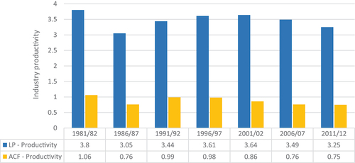
Using the production function estimates, LP and ACF TFP are derived from Equations (14)(14) $TF{P}_{it}=y_{it}-{\hat{\alpha }}_l{l}_{it}-{\hat{\alpha }}_k{k}_{it}-{\hat{\alpha }}_m{m}_{it}-{\hat{\alpha }}_f{f}_{it}-{\hat{\alpha }}_e{e}_{it}$(14) and (15(15) $TF{P}_{it}=v{a}_{it}-{\hat{\alpha }}_l{l}_{it}-{\hat{\alpha }}_k{k}_{it}$(15) ), respectively. In Figure 1, the two productivity measures for the Nepalese manufacturing sector from 1981/82 to 2011/12 are presented. Looking at ACF productivity first, the 1981/82 number is the highest at 1.06. Except for the increase from 1986/87 to 1991/92, the productivity measure gradually decreases over time, falling to 0.75 in 2011/12. In comparison, LP productivity displays a slightly different trend. The productivity number drops initially, as is the case with ACF productivity. It increases gradually from 1986/87 to 2001/02, after which the trend is reversed. This is consistent with the various domestic shocks that the Nepalese economy experienced during the study period. Between 1986/87 and 1996/97, LP productivity on average rises by 8.86%, but the productivity growth rate falls abruptly to 0.83% after 1996/97. One of the major reasons is due to the Maoist insurgency in 1996. In 2001, another domestic shock, the royal massacre, hit the economy badly; this is reflected in the decline of LP productivity by 4.12% after 2001/02.

Figure 1. LP and ACF total factor productivity.

5.2. Trade Policy Impact on Industry Productivity

Using LP and ACF productivity, each TFP measure is regressed on contemporaneous tariff rates (AHS and MFN tariffs separately) together with industry size and location. As the tariff data from the TRAINS database are available for Nepal only from 1990, this is the starting year for the trade-productivity estimation. Equation (16)(16) $TF{P}_{it}={\beta }_0+{\beta }_{1}tarif{f}_{it}+\beta {{ }^{\mathrm{\prime }}}_{2}ind\mathrm{\_}du{m}_{it}+\beta {{ }^{\mathrm{\prime }}}_3{\left(tariff\times ind\mathrm{\_}dum\right)}_{it}+{\eta }_i+{\lambda }_t+{\epsilon }_{it}$(16) is estimated in four specifications (M1-M4) with industry- and year-fixed effects and the results are reported in Table 3 (LP productivity) and Table 4 (ACF productivity). Starting with LP productivity and AHS tariff rates in Table 3, the first model M1 regresses TFP on tariffs only. While the coefficient shows the expected negative sign, i.e., lower tariffs increase industry productivity; however, it is not statistically significant. In fact, the tariff coefficient is also negative and insignificant in M2-M4. In M2, two industrial characteristic indicator variables are included. Although the coefficients are not significant, the estimated sign suggests that large industries benefit from efficiency scale in lifting productivity. Separately, industries that are located in rural areas suffer from falling productivity. Progressing to M3, it is additionally assessed whether tariffs affect TFP differently depending on industry characteristics. Hence, two more regressors are added: tariffs interact, respectively, with (“Large”) size and (“Rural”) location variables. Interestingly, while tariffs do not affect productivity directly, its interactive term with size (large industries) is negative and significant at 1%. This suggests that productivity enhancement from lower tariffs is concentrated in large industries than diffused across the entire manufacturing sector in Nepal. The large industries coefficient now indicates a significant (at 10%) and very strong positive effect on industry productivity, i.e., 1% expansion of large industries (relative to small industries) in the manufacturing sector improves productivity by 235%.⁹

Table 3. Tariff impact on LP industry productivity.

	AHS Tariffs				MFN Tariffs
Dep. variable: LP TFP	M1	M2	M3	M4	M1	M2	M3	M4
Tariffs	−0.0213	−0.0208	−0.0006	−0.0032	−0.0189	−0.0175	−0.0004	−0.0034
	(0.0159)	(0.0156)	(0.0085)	(0.0079)	(0.0250)	(0.0250)	(0.0124)	(0.0113)
Large Ind		0.1575	1.2079*	1.2738**		0.1566	1.2509*	1.3016**
		(0.3460)	(0.6323)	(0.6362)		(0.3378)	(0.6925)	(0.6260)
Rural Ind		−0.1804	0.0787	0.0923		−0.1639	−0.0332	−0.0259
		(0.1342)	(0.3757)	(0.3672)		(0.1155)	(0.4748)	(0.4482)
Tariffs×Large Ind			−0.0635***	−0.0504**			−0.0633**	−0.0493*
			(0.0224)	(0.0246)			(0.0296)	(0.0286)
Tariffs×Rural Ind			−0.0214	−0.0174			−0.0118	−0.0074
			(0.0191)	(0.0196)			(0.0254)	(0.0240)
Tariffs×Large Ind×Rural Ind				−0.0309*				−0.0301
				(0.0158)				(0.0272)
Industry-fixed effects	Yes	Yes	Yes	Yes	Yes	Yes	Yes	Yes
Year-fixed effects	Yes	Yes	Yes	Yes	Yes	Yes	Yes	Yes
R^2	0.046	0.049	0.091	0.097	0.034	0.037	0.071	0.077
N observations	283	283	283	283	298	298	298	298

Note: Robust standard errors clustered by industry are in parentheses. LP TFP is Levinsohn-Petrin total factor productivity; AHS is effectively applied tariff; MFN is most favored nations tariff. *p < .10, **p < .05, and ***p < .01 denote statistical significance at 10%, 5%, and 1% respectively.

Table 4. Tariff impact on ACF industry productivity.

`	AHS Tariffs				MFN Tariffs
Dep. variable: ACF TFP	M1	M2	M3	M4	M1	M2	M3	M4
Tariffs	−0.0048	−0.0048	0.0022	0.0012	−0.0013	−0.0011	0.0026	0.0019
	(0.0046)	(0.0046)	(0.0044)	(0.0046)	(0.0062)	(0.0061)	(0.0056)	(0.0057)
Large Ind		0.0136	0.0754	0.1016		0.0061	−0.0132	−0.0011
		(0.0999)	(0.1378)	(0.1318)		(0.0907)	(0.1701)	(0.1658)
Rural Ind		−0.0370	0.1441	0.1495		−0.0344	0.0881	0.0898
		(0.0833)	(0.1517)	(0.1513)		(0.0734)	(0.1572)	(0.1550)
Tariffs×Large Ind			−0.0055	−0.0003			−0.0001	0.0032
			(0.0048)	(0.0047)			(0.0062)	(0.0068)
Tariffs×Rural Ind			−0.0107*	−0.0091			−0.0071	−0.0060
			(0.0062)	(0.0063)			(0.0072)	(0.0075)
Tariffs×Large Ind×Rural Ind				−0.0123*				−0.0072
				(0.0064)				(0.0061)
Industry-fixed effects	Yes	Yes	Yes	Yes	Yes	Yes	Yes	Yes
Year-fixed effects	Yes	Yes	Yes	Yes	Yes	Yes	Yes	Yes
R^2	0.067	0.068	0.078	0.084	0.059	0.059	0.062	0.064
N observations	283	283	283	283	298	298	298	298

Note: Robust standard errors clustered by industry are in parentheses. ACF TFP is Ackerberg-Caves-Frazer total factor productivity; AHS is effectively applied tariff; MFN is most favored nations tariff. *p < .10, **p < .05, and ***p < .01 denote statistical significance at 10%, 5%, and 1% respectively.

Given the large estimated productivity effects in M3 that go toward large industries, estimation is further extended to M4 with another regressor where both size and location interact with tariffs to uncover any additional liberalization effect that may lead to further productivity boost for large industries operating in rural areas. The results show that while the significant estimates for large industries increasing productivity through size and tariff reduction effects continue to be present, there is further productivity enhancement for rural-based large industries, i.e., productivity rises by 0.3% with a 10% tariff reduction. Switching to MFN tariffs, the results are consistent with those of AHS tariffs in that productivity increases are due to large industry size effect and lower tariff effect from trade policy. However, the additional tariff effect that improves productivity specifically for large, rural industries is not significant.

For robustness check, Equation (16)(16) $TF{P}_{it}={\beta }_0+{\beta }_{1}tarif{f}_{it}+\beta {{ }^{\mathrm{\prime }}}_{2}ind\mathrm{\_}du{m}_{it}+\beta {{ }^{\mathrm{\prime }}}_3{\left(tariff\times ind\mathrm{\_}dum\right)}_{it}+{\eta }_i+{\lambda }_t+{\epsilon }_{it}$(16) is estimated using ACF productivity, and the results are reported in Table 4. With AHS tariffs, the estimated coefficients show consistently that large industries reap the benefit of higher productivity when tariffs are lowered (significant at 10% in M3). Additional productivity gains are accrued to large industries operating in rural areas (at 10% significance level in M4). As a result, large industries are able to reduce costs because of operational scale and better at withstanding external competition shocks. Using MFN tariffs, the story is qualitatively consistent with the estimated coefficients bearing the expected negative sign but not significant. The policy implication from these results is that small industries, irrespective of their location, would need time and require government policy assistance to increase productivity in the face of new foreign competition introduced by trade liberalization.

5.3. Trade Policy Impact by Productivity Quantiles

The empirical analysis so far focuses on how the conditional mean level of industry productivity would change in response to different levels of trade protection. This may not be sufficient to uncover variations in responses depending on where industries are situated in the productivity distribution, i.e., more efficient industries may respond differently to trade policy compared to less efficient industries (Kealey, Pujolas, and Sosa‐Padilla 2019). To understand more on this potential asymmetry in the trade-productivity nexus, the present study conducts a quantile regression analysis using the estimator developed by Powell (2022). Table 5 reports quantile regression estimates in which the dependent variable of logged industry productivity is regressed on logged 4-digit industry-level import tariffs, including both year- and industry-fixed effects. For each of the LP and ACF productivity measures, both AHS and MFN tariffs are used to examine their impacts on industry productivity at different quantiles.

Table 5. Impact of tariffs on industry productivity quantiles.

	LP TFP		ACF TFP
	AHS	MFN	AHS	MFN
q10	0.0032	0.0057	−0.0016	−0.0067
	(0.0048)	(0.0092)	(0.0067)	(0.0208)
q25	−0.0065	−0.0060	−0.0057	−0.0040
	(0.0076)	(0.0082)	(0.0076)	(0.0110)
q50	−0.0082	−0.0151	−0.0056	−0.0034
	(0.0094)	(0.0162)	(0.0043)	(0.0069)
q75	−0.0101	−0.0088	−0.0019	0.0024
	(0.0074)	(0.0076)	(0.0077)	(0.0083)
q90	−0.0587***	−0.0289*	−0.0140	−0.0164
	(0.0136)	(0.0154)	(0.2700)	(0.0230)
q95			−0.1568***	0.0073
			(0.0459)	(0.0074)

Note: Standard errors are in parentheses. TFP is total factor productivity; LP stands for Levinsohn and Petrin (2003); ACF stands for Ackerberg, Caves, and Frazer (2015); AHS is effectively applied tariff; MFN is most favored nations tariff. *p < .10, **p < .05, and ***p < .01 denote statistical significance at 10%, 5%, and 1% respectively. q10 to q95 denote productivity distribution at different quantiles. All specifications of quantile regressions include both year- and industry-fixed effects.

The results generally show that most of the coefficient estimates are negative for both tariffs with respect to LP and ACF productivity, confirming that lower tariffs lead to higher productivity. In addition, regardless of the productivity and tariff measures used in the quantile regression, there is an increasingly negative relationship between industry productivity and tariff reductions when moving from lower to upper quantiles of the productivity distribution. This suggests that much of the productivity growth due to trade liberalization is taking place among the industries that were already the most productive ones in their respective groups. Examining the tariff coefficients under LP productivity more closely, the sign starts as positive for the first quintile (q10) but changes to the expected negative sign from the first quartile (q25). This is the case, however, only for those industries that exhibit very high levels of productivity in the top decile (q90) that significant productivity improvement from tariff reductions is found (1% significant for AHS tariffs and 10% for MFN tariffs). Similarly, for ACF productivity, only the most efficient industries are found to enjoy productivity gains when trade protection is lowered. In fact, these would be industries operating in the 95^th quantile (q95) where the AHS tariff coefficient is significant at 1%. It is important to remember that a negative coefficient for trade policy variables (AHS and MFN tariffs) means that trade liberalization is productivity-enhancing. Industries at higher productivity ranges are shown to benefit from trade liberalization. This means more productive industries gain more from trade liberalization than less productive industries. According to Aghion et al. (2005), trade liberalization induces more productive industries to increase their investment in technology adoption in response to the threat of external competition.¹⁰ Hence, the results are consistent with Kealey, Pujolas, and Sosa‐Padilla (2019) in that the benefits of trade liberalization are accrued asymmetrically to industries situated only in the top decile of the productivity distribution.

5.4. Appropriateness of Quantile Regression (QRPD)

In this study, the major interest lies in estimating quantile treatment effects (QTEs) of trade policy changes $\left(x_{it}\right)$ on industry productivity improvements $\left(y_{it}\right)$ in Nepal. Existing quantile panel additive fixed effects models estimate, conditioning on industry fixed effects $\left({\eta }_i\right)$, the distribution of $\left.\left(y_{it}-{\eta }_i\right)\right|x_{it}$ instead of the distribution of $\left.y_{it}\right|x_{it}$. In the current study, the former result is undesirable since observations near the top of the $\left(y_{it}-{\eta }_i\right)$ distribution can be near the bottom of the $y_{it}$ distribution. Therefore, additive fixed effects models are unable to provide true information about trade policy effects on productivity distribution (Powell 2022). According to Powell (2022), these models can only provide information regarding the productivity-relative-to-fixed-effect distribution. However, the QRPD estimator utilized in this study estimates the distribution of interest, $\left(\left.y_{it}\right|x_{it}\right)$, that uncovers the heterogenous responses along the productivity quantile for tariff reductions.¹¹ These heterogenous responses are evident in the estimated results (Table 5) and show that only the upper part of the productivity distribution (at quantile 90) is responsive to trade policy changes.

In terms of competing quantile panel regression methodologies, Table 6 reports the mean absolute deviations (MAD), mean absolute error (MAE), and root mean squared error (RMSE) to compare the forecast performance of the Machado and Silva (2019) additive FE model and the Powell (2022) nonadditive FE model. The numbers show that the QRPD performs well throughout the distribution except for the last quantile. For 80% of the observed quantiles, the QRPD values for the three metrics are less than those for Machado and Silva (2019). These results relate to the appropriateness of using the QRPD estimator for quantile estimation.

Table 6. Quantile regression methodology comparison.

	Powell’s (2022) Nonadditive FE			Machado and Silva (2019) Additive FE
Quantiles	MAD	MAE	RMSE	MAD	MAE	RMSE
10	2.990	3.449	3.783	3.296	3.718	4.049
25	3.194	3.63	3.961	3.335	3.746	4.078
50	3.230	3.661	3.993	3.387	3.788	4.119
75	3.261	3.696	4.027	3.444	3.839	4.171
90	4.095	4.598	4.966	3.475	3.871	4.204

Note: MAD = Median Absolute Deviation, MAE = Mean Absolute Error, RMSE = Root Mean Squared Error.

6. Discussion

The findings of this study suggest that only large industries in the Nepalese manufacturing sector derive productivity gains from trade liberalization. First, estimates indicate that an expansion in the size of the large industry cohort raises overall productivity as they are able to operate with efficiency scale and reduce costs. Second, increases in productivity as a result of tariff reductions are concentrated in large industries than diffused evenly across all industries in the manufacturing sector. This study also examines heterogeneity in trade policy impacts at different productivity quantiles and evidence that trade liberalization benefits are accrued significantly only to the most efficient industries in the top decile of the productivity distribution. This is consistent with Aghion et al. (2005) who assert that trade liberalization induces more productive industries to increase investment in technology adoption in response to the threat of external competition. The incentives for investment in technology adoption and R&D may intensify or diminish with trade liberalization, depending on whether the “scale effect” or the “competition effect” is more powerful (Grossman and Helpman 2015). Since the scale effect boosts the incentive for innovation and the competition effect provides an offsetting disincentive, the results of the study seem to support the former effect for the Nepalese manufacturing sector. The current study also evidences considerable heterogeneity in how the fruits of productivity improvement are shared between different types of industries in a trade liberalizing country. Benefits are found to be mainly attributable to large and more efficient industries. In fact, the Nepalese manufacturing sector is dominated by small industries, where large industries only make up around 16% of the sector. This suggests that Nepal still has much to gain from trade liberalization, especially via changes in industry composition as small industries grow in scale and size over time. Government and policymakers should work toward creating and facilitating an environment conducive to large-scaled investments in the manufacturing sector to ramp up the scale effect for industries to derive the most liberalization gain. Therefore, foreign direct investment (FDI), especially for a trade liberalizing economy, is considered critical as it can be a conduit for both large investments and knowledge transfer (Grossman and Helpman 2015). Currently, Nepal has only received US$0.13 billion FDI inflows, which ranks the lowest in South Asia. There is a huge gap between approved FDI and actual net FDI inflow in Nepal; between 1995/96 and 2019/20, total actual net FDI inflow was only 34.1% of the total approval (NRB 2021). Another important factor is the reduction of trade costs to further elevate trade liberalization gains. For a least developed country like Nepal, where the majority of industries are still fledgling, high trade cost demotivates engagement with foreign partners, thus preventing transfer of new knowledge and technologies into the country. Addressing the FDI inflow gap and alleviating costs and complexities of lengthy border procedures and controls should therefore be priority for policymakers in Nepal.

7. Conclusions

For small open developing economies employing trade liberalization as a tool to lift economic growth, one may hope that the process bears fruits that will be uniformly shared by all industries in the country. This paper examines the trade-productivity nexus looking at manufacturing industries in Nepal. Micro-level evidence is provided to show that trade liberalization impacts are industry-specific depending on industry characteristics and productivity distribution. The first set of results shows that only large industries derive productivity gains with lowered trade protection as part of the liberalization process. As Nepal’s manufacturing sector is dominated by small industries, the results suggest that there is ample opportunity for the sector to continue gaining from trade liberalization as different manufacturing industries become larger and more efficient over time. Since the scale effect boosts the incentive for innovation, new technology adoption, and R&D, increasing the size of the large industry cohort in Nepal is an important step in reaping further benefits from trade liberalization.

When industries are differentiated by productivity quantiles, the second set of results indicates that only the most efficient producers are able to take advantage of tariff reductions in generating significant productivity increases. The results show that trade liberalization impacts are heterogenous along the productivity distribution, where the traditional mean productivity approach is not able to uncover the asymmetric relationship between trade and productivity. The study also demonstrates that country-specific studies are able to utilize fundamental characteristics of a country, including its factors and resource endowments and history, to understand the mechanisms in which trade liberalization drives productivity growth.

Acknowledgements

We gratefully acknowledge the insightful comments and suggestions of two anonymous reviewers and the Subject Editor. This article is based on first author’s PhD dissertation research at the University of New England. Amrit Pathak also acknowledges financial support through the Australian Government Research Training Program Scholarship.

Disclosure Statement

No potential conflict of interest was reported by the author(s).

Notes

1. See, for example, Pavcnik (2002); Amiti and Konings (2007); Fernandes (2007); Topalova and Khandelwal (2011).

2. The implicit assumption with estimating industry-level production function is that all establishments in the Nepalese manufacturing industry are constrained to have the same technology. While it may be preferable to conduct the estimation at the establishment level, we are constrained by data availability since individual establishments are not uniquely identified in the national manufacturing census. Please see Section 4.3 for more data discussion.

3. Ackerberg, Caves, and Frazer (2015) recommend using their method only with value-added production function as there is no guarantee that gross output production function will be identified (Manjón and Mañez 2016).

4. The intermediate inputs that appear in Equation (5)(5) $y_{it}={\alpha }_l{l}_{it}+{\alpha }_k{k}_{it}+{\alpha }_m{m}_{it}+{\alpha }_f{f}_{it}+{\alpha }_e{e}_{it}+{\omega }_{it}+{\upsilon }_{it}$(5) are subtracted from total output to derive value-added output.

5. Powell (2022) states that in many economic applications, it is typical to have only one or two treatment variables, not counting fixed effects.

6. The occurrence of small observation numbers is mainly due to two reasons: First, there were three different industrial classification revisions that took place in Nepal from 1991/92 to 2011/12, where these modifications of the NSIC classification system were designed to be consistent with changes in the International Standard Industrial Classification of All Economic Activities. Hence one would suspect that the affected industries, that were under the same classification in earlier censuses, may have been assigned new codes in the revised classification, given the fact that they belong to the same 3-digit classification today. The second reason could be due to new entry into the market.

7. See Table A1 in the Appendix for descriptive statistics on productivity and tariff measures and Table A2 on production function variables.

8. Overall, the sector contributes 36% of GDP (Ministry of Finance 2007).

9. Given the logarithmic TFP dependent variable, the percentage differential effect of large industries (relative to small industries) on productivity is $100\left(e{}^{{\hat{\beta }}_2}-1\right)\mathrm{\%}=100\left(e^{1.2079}-1\right)\mathrm{\%}=235\mathrm{\%}$.

10. Acemoglu (2003) argues that such technological adoption in the case of developing countries may take the form of increased import of machines, office equipment, and capital goods.

11. For more detailed information on the QRPD econometric setup and its distinction from the other quantile panel data estimators, see Powell (2022).

Appendix.

Descriptive Statistics.

Table A1. Productivity and tariffs measures.

Variables	Obs	Mean	Std. Dev.	Min	Max
LP TFP	298	3.488	1.535	1.635	13.406
ACF TFP	298	0.857	0.631	−0.846	3.021
AHS Tariffs	283	18.535	12.425	0.000	110.000
MFN Tariffs	298	17.847	10.499	1.560	71.670

Table A2. Production function variables.

Variables	Obs	Mean	Std. Dev.	Min	Max
Output	365	9.077	1.622	4.219	12.590
Value Added	365	7.942	1.619	3.483	11.491
Labor	365	6.458	1.459	2.445	10.470
Capital	365	8.149	1.669	2.983	12.061
Raw Materials	365	8.458	1.652	3.376	12.398
Fuel	365	4.827	2.075	−1.720	10.355
Electricity	365	4.703	1.848	−2.413	9.161

Table A3. Industry location and size characteristics.

Location	Size		Total
	Small	Large
Rural	89	39	128
Urban	160	10	170
Total	249	49	298

References

- Abegaz, B., and A. K. Basu. 2011. The elusive productivity effect of trade liberalisation in the manufacturing industries of emerging economies. Emerging Markets Finance and Trade 47 (1):5–27. doi:10.2753/REE1540-496X470101.
- Acemoglu, D. 2003. Patterns of skill premia. The Review of Economic Studies 70 (2):199–230. doi:10.1111/1467-937X.00242.
- Ackerberg, D. A., K. Caves, and G. Frazer. 2015. Identification properties of recent production function estimators. Econometrica 83 (6):2411–51. doi:10.3982/ECTA13408.
- Aghion, P., R. Burgess, S. Redding, and F. Zilibotti. 2005. Entry liberalisation and inequality in industrial performance. Journal of the European Economic Association 3 (2–3):291–302. doi:10.1162/jeea.2005.3.2-3.291.
- Ahmed, G., M. A. Khan, T. Mahmood, and M. Afzal. 2017. Trade liberalisation and industrial productivity: Evidence from manufacturing industries in Pakistan. Pakistan Development Review 56 (4):319–48. doi:10.30541/v56i4pp.319-348.
- Amiti, M., and J. Konings. 2007. Trade liberalisation, intermediate inputs, and productivity: Evidence from Indonesia. The American Economic Review 97 (5):1611–38. doi:10.1257/aer.97.5.1611.
- Beckmann, M., T. Cornelissen, and M. Kräkel. 2017. Self-managed working time and employee effort: Theory and evidence. Journal of Economic Behaviour & Organisation 133:285–302. doi:10.1016/j.jebo.2016.11.013.
- Biggs, T., J. Nasir, K. Pandey, and L. Zhao. 2000. The business environment and manufacturing performance in Nepal. World Bank and FNCCI, December, II, 3.
- Clemens, M. A., and J. G. Williamson. 2004. Why did the tariff-growth correlation change after 1950? Journal of Economic Growth 9 (1):5–46. doi:10.1023/B:JOEG.0000023015.44856.a9.
- Dastidar, S. G. 2015. Manufacturing and trade liberalisation of India: The continuing debate. Review of Development and Change 20 (2):225–44. doi:10.1177/0972266120150211.
- Edwards, S. 1998. Openness, productivity and growth: What do we really know? The Economic Journal 108 (447):383–98. doi:10.1111/1468-0297.00293.
- Ericson, R., and A. Pakes. 1995. Markov-perfect industry dynamics: A framework for empirical work. The Review of Economic Studies 62 (1):53–82. doi:10.2307/2297841.
- Fernandes, A. M. 2007. Trade policy, trade volumes and plant-level productivity in Colombian manufacturing industries. Journal of International Economics 1 (71):52–71. doi:10.1016/j.jinteco.2006.03.003.
- Goldberg, P. K., and N. Pavcnik. 2005. Trade, wages, and the political economy of trade protection: Evidence from the Colombian trade reforms. Journal of International Economics 66 (1):75–105. doi:10.1016/j.jinteco.2004.04.005.
- Greenaway, D., W. Morgan, and P. Wright. 2002. Trade liberalisation and growth in developing countries. Journal of Development Economics 67 (1):229–44. doi:10.1016/S0304-3878(01)00185-7.
- Grossman, G. M., and E. Helpman. 1991. Innovation and growth in the global economy. Cambridge, Massachusetts London: MIT press.
- Grossman, G. M., and E. Helpman. 1994. Endogenous innovation in the theory of growth. Journal of Economic Perspectives 8 (1):23–44. doi:10.1257/jep.8.1.23.
- Grossman, G. M., and E. Helpman. 2015. Globalisation and growth. The American Economic Review 105 (5):100–04. doi:10.1257/aer.p20151068.
- Harrison, A. E. 1994. Productivity, imperfect competition and trade reform: Theory and evidence. Journal of International Economics 36 (1–2):53–73. doi:10.1016/0022-1996(94)90057-4.
- Helpman, E., and P. R. Krugman. 1989. Trade policy and market structure. Cambridge, Massachusetts: MIT press.
- Kealey, J., P. S. Pujolas, and C. Sosa‐Padilla. 2019. Trade liberalisation and firm productivity: Estimation methods matter. Economic Inquiry 57 (3):1272–83. doi:10.1111/ecin.12767.
- Kneller, R., C. W. Morgan, and S. Kanchanahatakij. 2008. Trade liberalisation and economic growth. The World Economy 31 (6):701–19. doi:10.1111/j.1467-9701.2008.01101.x.
- Krueger, A. O. 1978. Foreign trade regimes and economic liberalization. Lexington, MA: Ballinger.
- Levinsohn, J., and A. Petrin. 2003. Estimating production functions using inputs to control for unobservables. The Review of Economic Studies 70 (2):317–41. doi:10.1111/1467-937X.00246.
- Machado, J. A., and J. S. Silva. 2019. Quantiles via moments. Journal of Econometrics 213 (1):145–73. doi:10.1016/j.jeconom.2019.04.009.
- Manjón, M., and J. Mañez. 2016. Production function estimation in Stata using the Ackerberg–Caves–Frazer method. The Stata Journal 16 (4):900–16. doi:10.1177/1536867X1601600406.
- Melitz, M. J. 2003. The impact of trade on intra‐industry reallocations and aggregate industry productivity. Econometrica 71 (6):1695–725. doi:10.1111/1468-0262.00467.
- Ministry of Finance. 2007. Source Book for Projects Financed with Foreign Assistance, Fiscal Year 2007–2008. Kathmandu: Government of Nepal.
- Muendler, M.-A. 2004. Trade, technology and productivity: A study of Brazilian manufacturers 1986-1998. CESifo Working Paper, No.1148.
- NRB. 2007. Inflation in Nepal. Research Department, Kathmandu, Nepal. https://www.nrb.org.np/contents/uploads/2020/11/Special_Publications-Inflation-in-Nepal.pdf.
- NRB. 2021. A survey report on foreign direct investment in Nepal. https://www.nrb.org.np/red/a-survey-report-on-foreign-direct-investment-in-nepal-2019-20/.
- Ogu, C., C. Aniebo, and P. Elekwa. 2016. Does Trade liberalisation hurt Nigeria’s manufacturing sector. International Journal of Economics and Finance 8 (6):175–80. doi:10.5539/ijef.v8n6p175.
- Olley, G. S., and A. Pakes. 1996. The dynamics of productivity in the telecommunications equipment industry. Econometrica 64 (6):1263. doi:10.2307/2171831.
- Pavcnik, N. 2002. Trade liberalisation, exit, and productivity improvements: Evidence from Chilean plants. The Review of Economic Studies 69 (1):245–76. doi:10.1111/1467-937X.00205.
- Powell, D. 2020. Does labour supply respond to transitory income? Evidence from the economic stimulus payments of 2008. Journal of Labour Economics 38 (1):1–38. doi:10.1086/704494.
- Powell, D. 2022. Quantile regression with nonadditive fixed effects. Empirical Economics 63 (5):1–17. doi:10.1007/s00181-022-02216-6.
- Redding, S. 2002. Path dependence, endogenous innovation, and growth. International Economic Review 43 (4):1215–48.
- Rijesh, R. 2020. Trade liberalisation, technology import, and Indian manufacturing exports. Global Economic Review 49 (4):369–95. doi:10.1080/1226508X.2020.1798267.
- Rivera-Batiz, L. A., and P. M. Romer. 1991. Economic integration and endogenous growth. The Quarterly Journal of Economics 106 (2):531–55. doi:10.2307/2937946.
- Rodriguez, F., and D. Rodrik. 2000. Trade policy and economic growth: A skeptic’s guide to the cross-national evidence. NBER Macroeconomics Annual 15:261–325. doi:10.1086/654419.
- Sachs, J. D., A. Warner, A. Åslund, and S. Fischer. 1995. Economic reform and the process of global integration. Brookings Papers on Economic Activity 1995 (1):1–118. doi:10.2307/2534573.
- Santos‐Paulino, A. U. 2005. Trade liberalisation and economic performance: Theory and evidence for developing countries. The World Economy 28 (6):783–821. doi:10.1111/j.1467-9701.2005.00707.x.
- Schor, A. 2004. Heterogeneous productivity response to tariff reduction: Evidence from Brazilian manufacturing firms. Journal of Development Economics 75 (2):373–96. doi:10.1016/j.jdeveco.2004.06.003.
- Sharma, G. D., M. I. Shah, U. Shahzad, M. Jain, and R. Chopra. 2021. Exploring the nexus between agriculture and greenhouse gas emissions in BIMSTEC region: The role of renewable energy and human capital as moderators. Journal of Environmental Management 297:113316. doi:10.1016/j.jenvman.2021.113316.
- Shrestha, R. S. 2010. Electricity crisis (load shedding) in Nepal, its manifestations and ramifications. Hydro Nepal: Journal of Water, Energy and Environment 6:7–17. doi:10.3126/hn.v6i0.4187.
- Smith, T. A. 2017. Do school food programs improve child dietary quality? American Journal of Agricultural Economics 99 (2):339–56. doi:10.1093/ajae/aaw091.
- Syverson, C. 2011. What determines productivity? Journal of Economic Literature 49 (2):326–65. doi:10.1257/jel.49.2.326.
- Topalova, P., and A. Khandelwal. 2011. Trade liberalisation and firm productivity: The case of India. The Review of Economics and Statistics 93 (3):995–1009. doi:10.1162/REST_a_00095.
- Trefler, D. 1993. Trade liberalisation and the theory of endogenous protection: An econometric study of US import policy. The Journal of Political Economy 101 (1):138–60. doi:10.1086/261869.
- Tybout, J., J. De Melo, and V. Corbo. 1991. The effects of trade reforms on scale and technical efficiency: New evidence from Chile. Journal of International Economics 31 (3–4):231–50. doi:10.1016/0022-1996(91)90037-7.
- Tybout, J. R., and M. D. Westbrook. 1995. Trade liberalization and the dimensions of efficiency change in Mexican manufacturing industries. Journal of International Economics 39 (1–2):53–78. doi:10.1016/0022-1996(94)01363-W.
- Wacziarg, R. 2001. Measuring the dynamic gains from trade. The World Bank Economic Review 15 (3):393–429. doi:10.1093/wber/15.3.393.
- WTO. 2012. Trade policy review - Nepal. https://www.wto.org/english/tratop_e/tpr_e/tp357_e.htm.
- Yu, M., G. Ye, and B. Qu. 2013. Trade liberalisation, product complexity and productivity improvement: Evidence from Chinese firms. The World Economy 36 (7):912–34. doi:10.1111/twec.12046.