Convexity criteria for expansions of the Landau-de Gennes elastic free energy

Abstract

The Landau-de Gennes elastic free energy of liquid crystals is a functional expressed in terms of a symmetric traceless tensor order parameter. We derive convexity criteria for SO(3)-invariant expansions of the elastic energy that are quadratic in the gradient and up to fourth-order overall in the tensor order parameter. To do so we write the integrand as the sum of squares of linearly independent spherical tensors from which definiteness criteria can be ascertained. In particular, transformations between Cartesian and spherical tensors representations are computed based on irreducible tensor representations of the rotation group.

Keywords:

• calculus of variations
• Clebsch–Gordan coefficients
• convexity
• Landau-de Gennes energy
• spherical tensor representations

1. Introduction

The orientational properties of liquid crystals for the nematic-isotropic transition may be specified, at each point $\mathit{r}$ in the medium, by a symmetric traceless 2-tensor $Q=Q(\mathit{r})$ of Cartesian components $Q_{\alpha \beta }(\mathit{r})$ ($\alpha ,\beta =x,y,z$). By definition, the tensor vanishes in the isotropic phase and thus serves as an order parameter. In a general nematic phase, the order parameter has five degrees of freedom (two specifying the degree order with the other three for the principal directions). To find the equilibrium state of the medium, one seeks a minimizer of the free energy functional. The existence of a minimizer is typically established using direct methods whereby the key requirement is for the functional to be weakly sequentially lower semicontinuous with respect to the Sobolev norm (cf. [1]). Thus, we seek to ascertain sufficient conditions (in the form of convexity conditions for the integrand) as a means of ensuring lower semicontinuity.

In Landau’s theory of phase transitions [2], the free energy is expanded as a function of the order parameter into powers of Q and its derivatives [3,4]. The expansion is subject to the condition that free energy is invariant under the rotation group SO(3) (which consists of real 3 × 3 matrices R that satisfy $R^{T}R=R{R}^T=I_3$ and have determinant 1). Thus we seek to minimize the elastic free energy part of the Landau-de Gennes functional of the form $$\mathfrak{F}(Q)={\int }_{\Omega }{f}_E(Q,\nabla Q) dV$$ on an open bounded domain $\Omega \subset {\mathbb{R}}^3$ for the medium. Note that a bulk-free energy term of the form $f_B(Q)$ is added to the elastic integrand $f_E(Q,\nabla Q),$ however, we are only concerned with the non-trivial free energy term that involves quadratic derivatives of Q. The addition of a typical bulk term is a trivial extension with regards to sufficient conditions for lower semicontinuity.

The elastic energy integrand f_E is subject to requirement that it is invariant under the group action $\star$ of SO(3) by conjugation, i.e. the action given by $${(R\star Q)}_{\alpha \beta }=R_{\alpha \mu }{R}_{\beta \nu }{Q}_{\mu \nu }\hspace{1em}\mathrm{ }\text{and}\mathrm{ }\hspace{1em}{(R\star \nabla Q)}_{\alpha \beta \gamma }=R_{\alpha \mu }{R}_{\beta \nu }{R}_{\gamma \rho }{Q}_{\mu \nu ,\rho }$$ for any $R\in SO(3).$*

The principal Landau-type expansion of the elastic energy into SO(3)-invariant terms quadratic in $\nabla Q$ takes the form (1) $$f_E^{(2)}(\nabla Q)=L_1 Q_{\alpha \beta ,\gamma }{Q}_{\alpha \beta ,\gamma }+L_2 Q_{\alpha \beta ,\beta }{Q}_{\alpha \gamma ,\gamma }+L_3 Q_{\alpha \beta ,\gamma }{Q}_{\alpha \gamma ,\beta }$$(1) with elastic constants L₁, L₂, and L₃. Note that there are only five possible contractions of a symmetric 2-tensor in the form $\nabla Q*\nabla Q$ (the other remaining two terms $Q_{\gamma \gamma ,\beta }{Q}_{\alpha \alpha ,\beta },$ and $Q_{\alpha \alpha ,\beta }{Q}_{\beta \gamma ,\gamma }$ are excluded by the traceless requirement).^† The associated surface relation (i.e. null Lagrangian) is given by $${\partial }_{\alpha }(Q_{\alpha \beta }{Q}_{\beta \gamma ,\gamma }-Q_{\beta \gamma }{Q}_{\alpha \beta ,\gamma })=Q_{\alpha \beta ,\beta }{Q}_{\alpha \gamma ,\gamma }-Q_{\alpha \beta ,\gamma }{Q}_{\alpha \gamma ,\beta }.$$

We remark that while de Gennes’ theory gives a simple expression for the Oseen–Frank elastic energy constants, the expansion given by Equation (1(1) $$f_E^{(2)}(\nabla Q)=L_1 Q_{\alpha \beta ,\gamma }{Q}_{\alpha \beta ,\gamma }+L_2 Q_{\alpha \beta ,\beta }{Q}_{\alpha \gamma ,\gamma }+L_3 Q_{\alpha \beta ,\gamma }{Q}_{\alpha \gamma ,\beta }$$(1) ) implies a degeneracy in the splay and bend constants; a degeneracy that is in clear contradiction with experiment (see, e.g. [5–7]).^‡ Hence the expansion of Equation (1)(1) $$f_E^{(2)}(\nabla Q)=L_1 Q_{\alpha \beta ,\gamma }{Q}_{\alpha \beta ,\gamma }+L_2 Q_{\alpha \beta ,\beta }{Q}_{\alpha \gamma ,\gamma }+L_3 Q_{\alpha \beta ,\gamma }{Q}_{\alpha \gamma ,\beta }$$(1) is deemed too simple to describe correctly elastic properties of real liquid-crystal materials.

One way to rectify this issue is to consider higher order SO(3)-invariant terms of the form $Q*\nabla Q*\nabla Q$ and $Q*Q*\nabla Q*\nabla Q,$ i.e. terms that are quadratic in the gradient and third or fourth-order overall in the tensor order parameter. A program along these lines has been carried out by [8–10] for such third-order invariants and extended to fourth-order by [11]. Using a brute-force-method developed in [12] we calculate all contractions of a particular tensorial expression and confirm that there are three invariants of the form $\nabla Q*\nabla Q,$ seven invariants of the form $Q*\nabla Q*\nabla Q$ , and nineteen invariants of the form $Q*Q*\nabla Q*\nabla Q$ for a symmetric traceless 2-tensor Q (cf. Appendix A). By doing so we find five additional invariants of the form $Q*Q*\nabla Q*\nabla Q$ that are previously not listed in [11]. There is also an additional complication residing in fact that there are a certain number of (not at all immediately obvious) linear dependences between terms of higher order invariants. In Appendix D, we show that there is a maximum of six linearly independent invariants of the form $Q*\nabla Q*\nabla Q$ and a maximum of thirteen linearly independent invariants of the form $Q*Q*\nabla Q*\nabla Q.$ We remark that the result of Theorem 2.5 below could, in principle, be extended to incorporate higher order terms of the form $Q*Q*Q*\nabla Q*\nabla Q$ and $Q*Q*Q*Q*\nabla Q*\nabla Q$ or indeed other systems in condensed matter physics with different order parameters (e.g. the order parameter of anisotropic superfluid liquid helium-3 in the Ginzburg–Landau regime [13, p. 541]).

By taking the first six invariants listing in Equation (59), we see that the third-order linearly independent SO(3)-invariant terms of the form $Q*\nabla Q*\nabla Q$ can be written out as a linear combination of the form (2) $$\begin{array}{cc}{f}_E^{(3)}(Q,\nabla Q)\hfill & =M_1 Q_{\alpha \beta }{Q}_{\alpha \beta ,\mu }{Q}_{\mu \nu ,\nu }+M_2 Q_{\alpha \beta }{Q}_{\alpha \mu ,\beta }{Q}_{\mu \nu ,\nu }\hfill \\ \hfill & \hspace{1em}+M_3 Q_{\alpha \beta }{Q}_{\alpha \mu ,\mu }{Q}_{\beta \nu ,\nu }+M_4 Q_{\alpha \beta }{Q}_{\alpha \mu ,\nu }{Q}_{\beta \mu ,\nu }\hfill \\ \hfill & \hspace{1em}+M_5 Q_{\alpha \beta }{Q}_{\alpha \mu ,\nu }{Q}_{\beta \nu ,\mu }+M_6 Q_{\alpha \beta }{Q}_{\alpha \mu ,\nu }{Q}_{\mu \nu ,\beta }\hfill \end{array}$$(2) with elastic constants $M_1,M_2,M_3,M_4,M_5,M_6$ and one surface relation given by $$\begin{array}{c}{\partial }_{\nu }\left(Q_{\alpha \beta }{Q}_{\alpha \mu }{Q}_{\beta \nu ,\mu }\right)-{\partial }_{\beta }\left(Q_{\alpha \beta }{Q}_{\alpha \mu }{Q}_{\mu \nu ,\nu }\right)=Q_{\alpha \beta }{Q}_{\alpha \mu ,\nu }{Q}_{\beta \nu ,\mu }+Q_{\alpha \beta }{Q}_{\alpha \mu ,\nu }{Q}_{\mu \nu ,\beta }\\ \hspace{1em} -Q_{\alpha \beta }{Q}_{\alpha \mu ,\beta }{Q}_{\mu \nu ,\nu }-Q_{\alpha \beta }{Q}_{\alpha \mu ,\mu }{Q}_{\beta \nu ,\nu }.\end{array}$$

In addition to the six invariants included in Equation (2)(2) $$\begin{array}{cc}{f}_E^{(3)}(Q,\nabla Q)\hfill & =M_1 Q_{\alpha \beta }{Q}_{\alpha \beta ,\mu }{Q}_{\mu \nu ,\nu }+M_2 Q_{\alpha \beta }{Q}_{\alpha \mu ,\beta }{Q}_{\mu \nu ,\nu }\hfill \\ \hfill & \hspace{1em}+M_3 Q_{\alpha \beta }{Q}_{\alpha \mu ,\mu }{Q}_{\beta \nu ,\nu }+M_4 Q_{\alpha \beta }{Q}_{\alpha \mu ,\nu }{Q}_{\beta \mu ,\nu }\hfill \\ \hfill & \hspace{1em}+M_5 Q_{\alpha \beta }{Q}_{\alpha \mu ,\nu }{Q}_{\beta \nu ,\mu }+M_6 Q_{\alpha \beta }{Q}_{\alpha \mu ,\nu }{Q}_{\mu \nu ,\beta }\hfill \end{array}$$(2) , the final invariant of the form (3) $$M_7 Q_{\alpha \beta }{Q}_{\mu \nu ,\alpha }{Q}_{\mu \nu ,\beta }$$(3) can be expressed as a linear combination of the other six terms, namely (4) $$M_7 Q_{\alpha \beta }{Q}_{\mu \nu ,\alpha }{Q}_{\mu \nu ,\beta }=f_E^{(3)}(Q,\nabla Q)$$(4) with (5) $$M_1=-2M_7,M_2=2M_7,M_3=M_7,M_4=-2M_7,M_5=M_7,M_6=2M_7.$$(5)

A computation of the linear dependencies in Equation (5)(5) $$M_1=-2M_7,M_2=2M_7,M_3=M_7,M_4=-2M_7,M_5=M_7,M_6=2M_7.$$(5) is given by Equation (61)(61) $$\left(\begin{array}{ccccccc}1& 0& 0& 0& 0& 0& 2\\ 0& 1& 0& 0& 0& 0& -2\\ 0& 0& 1& 0& 0& 0& -1\\ 0& 0& 0& 1& 0& 0& 2\\ 0& 0& 0& 0& 1& 0& -1\\ 0& 0& 0& 0& 0& 1& -2\end{array}\right)$$(61) in Appendix D.1. We remark that the relations given by Equation (5)(5) $$M_1=-2M_7,M_2=2M_7,M_3=M_7,M_4=-2M_7,M_5=M_7,M_6=2M_7.$$(5) with $M_7=0$ also show that the six terms in Equation (2)(2) $$\begin{array}{cc}{f}_E^{(3)}(Q,\nabla Q)\hfill & =M_1 Q_{\alpha \beta }{Q}_{\alpha \beta ,\mu }{Q}_{\mu \nu ,\nu }+M_2 Q_{\alpha \beta }{Q}_{\alpha \mu ,\beta }{Q}_{\mu \nu ,\nu }\hfill \\ \hfill & \hspace{1em}+M_3 Q_{\alpha \beta }{Q}_{\alpha \mu ,\mu }{Q}_{\beta \nu ,\nu }+M_4 Q_{\alpha \beta }{Q}_{\alpha \mu ,\nu }{Q}_{\beta \mu ,\nu }\hfill \\ \hfill & \hspace{1em}+M_5 Q_{\alpha \beta }{Q}_{\alpha \mu ,\nu }{Q}_{\beta \nu ,\mu }+M_6 Q_{\alpha \beta }{Q}_{\alpha \mu ,\nu }{Q}_{\mu \nu ,\beta }\hfill \end{array}$$(2) are linearly independent of one another. In this way, Equation (2(2) $$\begin{array}{cc}{f}_E^{(3)}(Q,\nabla Q)\hfill & =M_1 Q_{\alpha \beta }{Q}_{\alpha \beta ,\mu }{Q}_{\mu \nu ,\nu }+M_2 Q_{\alpha \beta }{Q}_{\alpha \mu ,\beta }{Q}_{\mu \nu ,\nu }\hfill \\ \hfill & \hspace{1em}+M_3 Q_{\alpha \beta }{Q}_{\alpha \mu ,\mu }{Q}_{\beta \nu ,\nu }+M_4 Q_{\alpha \beta }{Q}_{\alpha \mu ,\nu }{Q}_{\beta \mu ,\nu }\hfill \\ \hfill & \hspace{1em}+M_5 Q_{\alpha \beta }{Q}_{\alpha \mu ,\nu }{Q}_{\beta \nu ,\mu }+M_6 Q_{\alpha \beta }{Q}_{\alpha \mu ,\nu }{Q}_{\mu \nu ,\beta }\hfill \end{array}$$(2) ) gives an expansion of SO(3)-invariant terms of the form $Q*\nabla Q*\nabla Q$ that is of full rank.

For fourth-order terms of the form $Q*Q*\nabla Q*\nabla Q,$ we can use the first thirteen invariants listing in Equation (60) to write the SO(3)-invariant expansion into linearly independent terms of the form (6) $$\begin{array}{cc}{f}_E^{(4)}(Q,\nabla Q)\hfill & =N_1 (\text{tr}\mathrm{ }{Q}^2)Q_{\rho \mu ,\rho }{Q}_{\mu \nu ,\nu }+N_2 (\text{tr}\mathrm{ }{Q}^2)Q_{\mu \nu ,\rho }{Q}_{\mu \nu ,\rho }\hfill \\ \hfill & \hspace{1em}+N_3 (\text{tr}\mathrm{ }{Q}^2)Q_{\mu \nu ,\rho }{Q}_{\rho \mu ,\nu }+N_4 Q_{\alpha \rho }{Q}_{\rho \beta }{Q}_{\alpha \beta ,\mu }{Q}_{\mu \nu ,\nu }\hfill \\ \hfill & \hspace{1em}+N_5 Q_{\alpha \rho }{Q}_{\rho \beta }{Q}_{\alpha \mu ,\beta }{Q}_{\mu \nu ,\nu }+N_6 Q_{\alpha \rho }{Q}_{\rho \beta }{Q}_{\alpha \mu ,\mu }{Q}_{\beta \nu ,\nu }\hfill \\ \hfill & \hspace{1em}+N_7 Q_{\alpha \rho }{Q}_{\beta \rho }{Q}_{\alpha \mu ,\nu }{Q}_{\beta \mu ,\nu }+N_8 Q_{\alpha \rho }{Q}_{\rho \beta }{Q}_{\alpha \mu ,\nu }{Q}_{\beta \nu ,\mu }\hfill \\ \hfill & \hspace{1em}+N_9 Q_{\alpha \rho }{Q}_{\rho \beta }{Q}_{\alpha \mu ,\nu }{Q}_{\mu \nu ,\beta }+N_{10} Q_{\alpha \beta }{Q}_{\mu \rho }{Q}_{\beta \mu ,\alpha }{Q}_{\rho \nu ,\nu }\hfill \\ \hfill & \hspace{1em}+N_{11} Q_{\alpha \beta }{Q}_{\mu \rho }{Q}_{\mu \nu ,\alpha }{Q}_{\rho \nu ,\beta }+N_{12} Q_{\alpha \beta }{Q}_{\mu \rho }{Q}_{\alpha \beta ,\nu }{Q}_{\nu \rho ,\mu }\hfill \\ \hfill & \hspace{1em}+N_{13} Q_{\alpha \beta }{Q}_{\mu \rho }{Q}_{\alpha \beta ,\nu }{Q}_{\mu \rho ,\nu }\hfill \end{array}$$(6) with elastic constants $N_1,\dots ,N_{13}$ and two surface relations given by $$\begin{array}{c}{\partial }_{\rho }(Q_{\rho \mu }{Q}_{\alpha \beta }{Q}_{\alpha \beta }{Q}_{\mu \nu ,\nu }-Q_{\mu \nu }{Q}_{\alpha \beta }{Q}_{\alpha \beta }{Q}_{\rho \mu ,\nu })\\ =-\left(\text{tr}\mathrm{ }{Q}^2\right)Q_{\mu \nu ,\rho }{Q}_{\rho \mu ,\nu }-2Q_{\alpha \rho }{Q}_{\rho \beta }{Q}_{\alpha \beta ,\mu }{Q}_{\mu \nu ,\nu }\\ \hspace{1em}+2Q_{\alpha \rho }{Q}_{\rho \beta }{Q}_{\alpha \mu ,\beta }{Q}_{\mu \nu ,\nu }+2Q_{\alpha \rho }{Q}_{\rho \beta }{Q}_{\alpha \mu ,\mu }{Q}_{\beta \nu ,\nu }\\ \hspace{1em}+2Q_{\alpha \beta }{Q}_{\mu \rho }{Q}_{\beta \mu ,\alpha }{Q}_{\rho \nu ,\nu }-2Q_{\alpha \beta }{Q}_{\mu \rho }{Q}_{\alpha \beta ,\nu }{Q}_{\nu \rho ,\mu }\end{array}$$ and $$\begin{array}{c}{\partial }_{\nu }\left(Q_{\beta \rho }{Q}_{\rho \alpha }{Q}_{\mu \nu }{Q}_{\alpha \mu ,\beta }\right)-{\partial }_{\beta }\left(Q_{\beta \rho }{Q}_{\rho \alpha }{Q}_{\mu \nu }{Q}_{\alpha \mu ,\nu }\right)\\ =-\frac{1}{2}\left(\text{tr}\mathrm{ }{Q}^2\right)Q_{\rho \mu ,\rho }{Q}_{\mu \nu ,\nu }+\frac{1}{2}\left(\text{tr}\mathrm{ }{Q}^2\right)Q_{\mu \nu ,\rho }{Q}_{\rho \mu ,\nu }\\ \hspace{1em}+3Q_{\alpha \rho }{Q}_{\rho \beta }{Q}_{\alpha \mu ,\beta }{Q}_{\mu \nu ,\nu }-3Q_{\alpha \rho }{Q}_{\rho \beta }{Q}_{\alpha \mu ,\nu }{Q}_{\mu \nu ,\beta }.\end{array}$$

In addition to the terms listed in Equation (6)(6) $$\begin{array}{cc}{f}_E^{(4)}(Q,\nabla Q)\hfill & =N_1 (\text{tr}\mathrm{ }{Q}^2)Q_{\rho \mu ,\rho }{Q}_{\mu \nu ,\nu }+N_2 (\text{tr}\mathrm{ }{Q}^2)Q_{\mu \nu ,\rho }{Q}_{\mu \nu ,\rho }\hfill \\ \hfill & \hspace{1em}+N_3 (\text{tr}\mathrm{ }{Q}^2)Q_{\mu \nu ,\rho }{Q}_{\rho \mu ,\nu }+N_4 Q_{\alpha \rho }{Q}_{\rho \beta }{Q}_{\alpha \beta ,\mu }{Q}_{\mu \nu ,\nu }\hfill \\ \hfill & \hspace{1em}+N_5 Q_{\alpha \rho }{Q}_{\rho \beta }{Q}_{\alpha \mu ,\beta }{Q}_{\mu \nu ,\nu }+N_6 Q_{\alpha \rho }{Q}_{\rho \beta }{Q}_{\alpha \mu ,\mu }{Q}_{\beta \nu ,\nu }\hfill \\ \hfill & \hspace{1em}+N_7 Q_{\alpha \rho }{Q}_{\beta \rho }{Q}_{\alpha \mu ,\nu }{Q}_{\beta \mu ,\nu }+N_8 Q_{\alpha \rho }{Q}_{\rho \beta }{Q}_{\alpha \mu ,\nu }{Q}_{\beta \nu ,\mu }\hfill \\ \hfill & \hspace{1em}+N_9 Q_{\alpha \rho }{Q}_{\rho \beta }{Q}_{\alpha \mu ,\nu }{Q}_{\mu \nu ,\beta }+N_{10} Q_{\alpha \beta }{Q}_{\mu \rho }{Q}_{\beta \mu ,\alpha }{Q}_{\rho \nu ,\nu }\hfill \\ \hfill & \hspace{1em}+N_{11} Q_{\alpha \beta }{Q}_{\mu \rho }{Q}_{\mu \nu ,\alpha }{Q}_{\rho \nu ,\beta }+N_{12} Q_{\alpha \beta }{Q}_{\mu \rho }{Q}_{\alpha \beta ,\nu }{Q}_{\nu \rho ,\mu }\hfill \\ \hfill & \hspace{1em}+N_{13} Q_{\alpha \beta }{Q}_{\mu \rho }{Q}_{\alpha \beta ,\nu }{Q}_{\mu \rho ,\nu }\hfill \end{array}$$(6) , there are a further six terms (i.e. the last six invariants listing in Equation (60)) of the form: (7) $$\begin{array}{cc}\hfill & N_{14} Q_{\alpha \rho }{Q}_{\rho \beta }{Q}_{\mu \nu ,\alpha }{Q}_{\mu \nu ,\beta }\hfill \\ \hfill & N_{15} Q_{\alpha \beta }{Q}_{\rho \mu }{Q}_{\mu \nu ,\beta }{Q}_{\alpha \nu ,\rho }\hfill \\ \hfill & N_{16} Q_{\alpha \beta }{Q}_{\rho \mu }{Q}_{\alpha \nu ,\beta }{Q}_{\rho \nu ,\mu }\hfill \\ \hfill & N_{17} Q_{\alpha \beta }{Q}_{\rho \mu }{Q}_{\alpha \beta ,\rho }{Q}_{\mu \nu ,\nu }\hfill \\ \hfill & N_{18} Q_{\alpha \beta }{Q}_{\rho \mu }{Q}_{\beta \nu ,\mu }{Q}_{\alpha \rho ,\nu }\hfill \\ \hfill & N_{19} Q_{\alpha \beta }{Q}_{\rho \mu }{Q}_{\beta \mu ,\nu }{Q}_{\alpha \rho ,\nu }\hfill \end{array}$$(7)

By setting (8) $$\begin{array}{cc}{f}_E^{(4)}(Q,\nabla Q)\hfill & =N_{14} Q_{\alpha \rho }{Q}_{\rho \beta }{Q}_{\mu \nu ,\alpha }{Q}_{\mu \nu ,\beta }+N_{15} Q_{\alpha \beta }{Q}_{\rho \mu }{Q}_{\mu \nu ,\beta }{Q}_{\alpha \nu ,\rho }\hfill \\ \hfill & \hspace{1em}+N_{16} Q_{\alpha \beta }{Q}_{\rho \mu }{Q}_{\alpha \nu ,\beta }{Q}_{\rho \nu ,\mu }+N_{17} Q_{\alpha \beta }{Q}_{\rho \mu }{Q}_{\alpha \beta ,\rho }{Q}_{\mu \nu ,\nu }\hfill \\ \hfill & \hspace{1em}+N_{18} Q_{\alpha \beta }{Q}_{\rho \mu }{Q}_{\beta \nu ,\mu }{Q}_{\alpha \rho ,\nu }+N_{19} Q_{\alpha \beta }{Q}_{\rho \mu }{Q}_{\beta \mu ,\nu }{Q}_{\alpha \rho ,\nu }\hfill \end{array}$$(8) a computation given in Appendix D.2 shows that (9) $$\begin{array}{c}{N}_1=-N_{14}-N_{15}-\frac{1}{2}{N}_{16}-\frac{1}{2}{N}_{17}\hfill \\ N_2=N_{14}+\frac{1}{2}{N}_{15}+\frac{1}{2}{N}_{16}+\frac{1}{2}{N}_{19}\hfill \\ N_3=-N_{14}-\frac{1}{2}{N}_{15}-N_{16}+\frac{1}{2}{N}_{18}\hfill \\ N_4=-2N_{14}-2N_{15}-2N_{16}-N_{17}+N_{18}\hfill \\ N_5=2N_{14}+2N_{15}+N_{17}\hfill \\ N_6=N_{14}+N_{15}+N_{16}+N_{17}\hfill \\ N_7=-2N_{14}-N_{15}-N_{16}-2N_{19}\hfill \\ N_8=N_{14}+N_{15}+N_{16}-N_{18}\hfill \\ N_9=2N_{14}+2N_{16}-N_{18}\hfill \\ N_{10}=N_{17}\hfill \\ N_{11}=N_{15}+N_{16}\hfill \\ N_{12}=N_{18}\hfill \\ N_{13}=N_{19}.\hfill \end{array}$$(9)

Therefore, the terms listed in Equation (7)(7) $$\begin{array}{cc}\hfill & N_{14} Q_{\alpha \rho }{Q}_{\rho \beta }{Q}_{\mu \nu ,\alpha }{Q}_{\mu \nu ,\beta }\hfill \\ \hfill & N_{15} Q_{\alpha \beta }{Q}_{\rho \mu }{Q}_{\mu \nu ,\beta }{Q}_{\alpha \nu ,\rho }\hfill \\ \hfill & N_{16} Q_{\alpha \beta }{Q}_{\rho \mu }{Q}_{\alpha \nu ,\beta }{Q}_{\rho \nu ,\mu }\hfill \\ \hfill & N_{17} Q_{\alpha \beta }{Q}_{\rho \mu }{Q}_{\alpha \beta ,\rho }{Q}_{\mu \nu ,\nu }\hfill \\ \hfill & N_{18} Q_{\alpha \beta }{Q}_{\rho \mu }{Q}_{\beta \nu ,\mu }{Q}_{\alpha \rho ,\nu }\hfill \\ \hfill & N_{19} Q_{\alpha \beta }{Q}_{\rho \mu }{Q}_{\beta \mu ,\nu }{Q}_{\alpha \rho ,\nu }\hfill \end{array}$$(7) are linearly dependent on the 13 terms listed in Equation (6)(6) $$\begin{array}{cc}{f}_E^{(4)}(Q,\nabla Q)\hfill & =N_1 (\text{tr}\mathrm{ }{Q}^2)Q_{\rho \mu ,\rho }{Q}_{\mu \nu ,\nu }+N_2 (\text{tr}\mathrm{ }{Q}^2)Q_{\mu \nu ,\rho }{Q}_{\mu \nu ,\rho }\hfill \\ \hfill & \hspace{1em}+N_3 (\text{tr}\mathrm{ }{Q}^2)Q_{\mu \nu ,\rho }{Q}_{\rho \mu ,\nu }+N_4 Q_{\alpha \rho }{Q}_{\rho \beta }{Q}_{\alpha \beta ,\mu }{Q}_{\mu \nu ,\nu }\hfill \\ \hfill & \hspace{1em}+N_5 Q_{\alpha \rho }{Q}_{\rho \beta }{Q}_{\alpha \mu ,\beta }{Q}_{\mu \nu ,\nu }+N_6 Q_{\alpha \rho }{Q}_{\rho \beta }{Q}_{\alpha \mu ,\mu }{Q}_{\beta \nu ,\nu }\hfill \\ \hfill & \hspace{1em}+N_7 Q_{\alpha \rho }{Q}_{\beta \rho }{Q}_{\alpha \mu ,\nu }{Q}_{\beta \mu ,\nu }+N_8 Q_{\alpha \rho }{Q}_{\rho \beta }{Q}_{\alpha \mu ,\nu }{Q}_{\beta \nu ,\mu }\hfill \\ \hfill & \hspace{1em}+N_9 Q_{\alpha \rho }{Q}_{\rho \beta }{Q}_{\alpha \mu ,\nu }{Q}_{\mu \nu ,\beta }+N_{10} Q_{\alpha \beta }{Q}_{\mu \rho }{Q}_{\beta \mu ,\alpha }{Q}_{\rho \nu ,\nu }\hfill \\ \hfill & \hspace{1em}+N_{11} Q_{\alpha \beta }{Q}_{\mu \rho }{Q}_{\mu \nu ,\alpha }{Q}_{\rho \nu ,\beta }+N_{12} Q_{\alpha \beta }{Q}_{\mu \rho }{Q}_{\alpha \beta ,\nu }{Q}_{\nu \rho ,\mu }\hfill \\ \hfill & \hspace{1em}+N_{13} Q_{\alpha \beta }{Q}_{\mu \rho }{Q}_{\alpha \beta ,\nu }{Q}_{\mu \rho ,\nu }\hfill \end{array}$$(6) . Moreover, if we set $N_1=\cdots =N_{13}=0$ in Equation (9)(9) $$\begin{array}{c}{N}_1=-N_{14}-N_{15}-\frac{1}{2}{N}_{16}-\frac{1}{2}{N}_{17}\hfill \\ N_2=N_{14}+\frac{1}{2}{N}_{15}+\frac{1}{2}{N}_{16}+\frac{1}{2}{N}_{19}\hfill \\ N_3=-N_{14}-\frac{1}{2}{N}_{15}-N_{16}+\frac{1}{2}{N}_{18}\hfill \\ N_4=-2N_{14}-2N_{15}-2N_{16}-N_{17}+N_{18}\hfill \\ N_5=2N_{14}+2N_{15}+N_{17}\hfill \\ N_6=N_{14}+N_{15}+N_{16}+N_{17}\hfill \\ N_7=-2N_{14}-N_{15}-N_{16}-2N_{19}\hfill \\ N_8=N_{14}+N_{15}+N_{16}-N_{18}\hfill \\ N_9=2N_{14}+2N_{16}-N_{18}\hfill \\ N_{10}=N_{17}\hfill \\ N_{11}=N_{15}+N_{16}\hfill \\ N_{12}=N_{18}\hfill \\ N_{13}=N_{19}.\hfill \end{array}$$(9) , an elementary computation shows that $N_{14}=\cdots =N_{19}=0.$ Hence, the terms listed in Equation (7)(7) $$\begin{array}{cc}\hfill & N_{14} Q_{\alpha \rho }{Q}_{\rho \beta }{Q}_{\mu \nu ,\alpha }{Q}_{\mu \nu ,\beta }\hfill \\ \hfill & N_{15} Q_{\alpha \beta }{Q}_{\rho \mu }{Q}_{\mu \nu ,\beta }{Q}_{\alpha \nu ,\rho }\hfill \\ \hfill & N_{16} Q_{\alpha \beta }{Q}_{\rho \mu }{Q}_{\alpha \nu ,\beta }{Q}_{\rho \nu ,\mu }\hfill \\ \hfill & N_{17} Q_{\alpha \beta }{Q}_{\rho \mu }{Q}_{\alpha \beta ,\rho }{Q}_{\mu \nu ,\nu }\hfill \\ \hfill & N_{18} Q_{\alpha \beta }{Q}_{\rho \mu }{Q}_{\beta \nu ,\mu }{Q}_{\alpha \rho ,\nu }\hfill \\ \hfill & N_{19} Q_{\alpha \beta }{Q}_{\rho \mu }{Q}_{\beta \mu ,\nu }{Q}_{\alpha \rho ,\nu }\hfill \end{array}$$(7) are linearly independent of one another. Furthermore, if we set $N_{14}=\cdots =N_{19}=0$ in Equation (9)(9) $$\begin{array}{c}{N}_1=-N_{14}-N_{15}-\frac{1}{2}{N}_{16}-\frac{1}{2}{N}_{17}\hfill \\ N_2=N_{14}+\frac{1}{2}{N}_{15}+\frac{1}{2}{N}_{16}+\frac{1}{2}{N}_{19}\hfill \\ N_3=-N_{14}-\frac{1}{2}{N}_{15}-N_{16}+\frac{1}{2}{N}_{18}\hfill \\ N_4=-2N_{14}-2N_{15}-2N_{16}-N_{17}+N_{18}\hfill \\ N_5=2N_{14}+2N_{15}+N_{17}\hfill \\ N_6=N_{14}+N_{15}+N_{16}+N_{17}\hfill \\ N_7=-2N_{14}-N_{15}-N_{16}-2N_{19}\hfill \\ N_8=N_{14}+N_{15}+N_{16}-N_{18}\hfill \\ N_9=2N_{14}+2N_{16}-N_{18}\hfill \\ N_{10}=N_{17}\hfill \\ N_{11}=N_{15}+N_{16}\hfill \\ N_{12}=N_{18}\hfill \\ N_{13}=N_{19}.\hfill \end{array}$$(9) , then $N_1=\cdots =N_{13}=0.$ Hence, the 13 terms listed in Equation (6)(6) $$\begin{array}{cc}{f}_E^{(4)}(Q,\nabla Q)\hfill & =N_1 (\text{tr}\mathrm{ }{Q}^2)Q_{\rho \mu ,\rho }{Q}_{\mu \nu ,\nu }+N_2 (\text{tr}\mathrm{ }{Q}^2)Q_{\mu \nu ,\rho }{Q}_{\mu \nu ,\rho }\hfill \\ \hfill & \hspace{1em}+N_3 (\text{tr}\mathrm{ }{Q}^2)Q_{\mu \nu ,\rho }{Q}_{\rho \mu ,\nu }+N_4 Q_{\alpha \rho }{Q}_{\rho \beta }{Q}_{\alpha \beta ,\mu }{Q}_{\mu \nu ,\nu }\hfill \\ \hfill & \hspace{1em}+N_5 Q_{\alpha \rho }{Q}_{\rho \beta }{Q}_{\alpha \mu ,\beta }{Q}_{\mu \nu ,\nu }+N_6 Q_{\alpha \rho }{Q}_{\rho \beta }{Q}_{\alpha \mu ,\mu }{Q}_{\beta \nu ,\nu }\hfill \\ \hfill & \hspace{1em}+N_7 Q_{\alpha \rho }{Q}_{\beta \rho }{Q}_{\alpha \mu ,\nu }{Q}_{\beta \mu ,\nu }+N_8 Q_{\alpha \rho }{Q}_{\rho \beta }{Q}_{\alpha \mu ,\nu }{Q}_{\beta \nu ,\mu }\hfill \\ \hfill & \hspace{1em}+N_9 Q_{\alpha \rho }{Q}_{\rho \beta }{Q}_{\alpha \mu ,\nu }{Q}_{\mu \nu ,\beta }+N_{10} Q_{\alpha \beta }{Q}_{\mu \rho }{Q}_{\beta \mu ,\alpha }{Q}_{\rho \nu ,\nu }\hfill \\ \hfill & \hspace{1em}+N_{11} Q_{\alpha \beta }{Q}_{\mu \rho }{Q}_{\mu \nu ,\alpha }{Q}_{\rho \nu ,\beta }+N_{12} Q_{\alpha \beta }{Q}_{\mu \rho }{Q}_{\alpha \beta ,\nu }{Q}_{\nu \rho ,\mu }\hfill \\ \hfill & \hspace{1em}+N_{13} Q_{\alpha \beta }{Q}_{\mu \rho }{Q}_{\alpha \beta ,\nu }{Q}_{\mu \rho ,\nu }\hfill \end{array}$$(6) are linearly independent of one another. In this way, we obtain an expansion given by Equation (6(6) $$\begin{array}{cc}{f}_E^{(4)}(Q,\nabla Q)\hfill & =N_1 (\text{tr}\mathrm{ }{Q}^2)Q_{\rho \mu ,\rho }{Q}_{\mu \nu ,\nu }+N_2 (\text{tr}\mathrm{ }{Q}^2)Q_{\mu \nu ,\rho }{Q}_{\mu \nu ,\rho }\hfill \\ \hfill & \hspace{1em}+N_3 (\text{tr}\mathrm{ }{Q}^2)Q_{\mu \nu ,\rho }{Q}_{\rho \mu ,\nu }+N_4 Q_{\alpha \rho }{Q}_{\rho \beta }{Q}_{\alpha \beta ,\mu }{Q}_{\mu \nu ,\nu }\hfill \\ \hfill & \hspace{1em}+N_5 Q_{\alpha \rho }{Q}_{\rho \beta }{Q}_{\alpha \mu ,\beta }{Q}_{\mu \nu ,\nu }+N_6 Q_{\alpha \rho }{Q}_{\rho \beta }{Q}_{\alpha \mu ,\mu }{Q}_{\beta \nu ,\nu }\hfill \\ \hfill & \hspace{1em}+N_7 Q_{\alpha \rho }{Q}_{\beta \rho }{Q}_{\alpha \mu ,\nu }{Q}_{\beta \mu ,\nu }+N_8 Q_{\alpha \rho }{Q}_{\rho \beta }{Q}_{\alpha \mu ,\nu }{Q}_{\beta \nu ,\mu }\hfill \\ \hfill & \hspace{1em}+N_9 Q_{\alpha \rho }{Q}_{\rho \beta }{Q}_{\alpha \mu ,\nu }{Q}_{\mu \nu ,\beta }+N_{10} Q_{\alpha \beta }{Q}_{\mu \rho }{Q}_{\beta \mu ,\alpha }{Q}_{\rho \nu ,\nu }\hfill \\ \hfill & \hspace{1em}+N_{11} Q_{\alpha \beta }{Q}_{\mu \rho }{Q}_{\mu \nu ,\alpha }{Q}_{\rho \nu ,\beta }+N_{12} Q_{\alpha \beta }{Q}_{\mu \rho }{Q}_{\alpha \beta ,\nu }{Q}_{\nu \rho ,\mu }\hfill \\ \hfill & \hspace{1em}+N_{13} Q_{\alpha \beta }{Q}_{\mu \rho }{Q}_{\alpha \beta ,\nu }{Q}_{\mu \rho ,\nu }\hfill \end{array}$$(6) ) of SO(3)-invariant terms of the form $Q*Q*\nabla Q*\nabla Q$ that is of full rank.

de Gennes’s original expression [4] for the expansion of the free-energy density in the absence of electric and magnetic fields also included a chiral term linear in the gradient of Q of the form ${\epsilon }_{\alpha \beta \gamma }{Q}_{\alpha \mu }{Q}_{\gamma \mu ,\beta }.$ Here, ${\epsilon }_{\alpha \beta \gamma }$ denotes the Levi-Civita tensor. For terms that are second order in $\nabla Q$ and up to fourth-order overall in the tensor order parameter there are three other chiral terms linear in the gradient of Q, namely those of the form ${\epsilon }_{\alpha \beta \gamma }{Q}_{\alpha \mu }{Q}_{\beta \nu }{Q}_{\mu \gamma ,\nu },{\epsilon }_{\alpha \beta \gamma }{Q}_{\alpha \mu }{Q}_{\beta \nu }{Q}_{\nu \rho }{Q}_{\mu \rho ,\gamma },$ and ${\epsilon }_{\alpha \beta \gamma }(\text{tr}\mathrm{ }{Q}^2)Q_{\alpha \rho }{Q}_{\gamma \rho ,\beta }$ (cf. [8,11,14]). We remark that these terms do not play a part in the integrand’s convexity, as per the condition of Equation (10)(10) $$f_{P_{\gamma }^{\alpha \beta }{P}_{\rho }^{\mu \nu }}(Q,P){\pi }_{\gamma }^{\alpha \beta }{\pi }_{\rho }^{\mu \nu }\ge l |\pi {|}^2$$(10) , due to the fact that they are only linear in the gradient of Q. Nevertheless, it is possible to consider further higher-order SO(3)-invariants terms like $Q*\cdots *Q*\nabla Q*\nabla Q$ which are quadratic in derivatives of Q (cf. [14]). Indeed, from the computations in Appendix A, we note that there are 36 invariants of the form $Q*Q*Q*\nabla Q*\nabla Q$ and 70 invariants of the form $Q*Q*Q*Q*\nabla Q*\nabla Q.$

When addressing the questions of the existence of a minimizer of the Landau-de Gennes elastic free energy functional, the convexity of the function $P\mapsto f_E(Q,P)$ and a coercivity requirement for f_E is a sufficient conditions for the existence of a minimizer of the functional $\mathfrak{F}$ in the class of Sobolev functions (cf. [15, Theorem 3.30]). Hence we want to equate the convexity of $f_E(Q, · )$ for the expansions given by the Equations (1(1) $$f_E^{(2)}(\nabla Q)=L_1 Q_{\alpha \beta ,\gamma }{Q}_{\alpha \beta ,\gamma }+L_2 Q_{\alpha \beta ,\beta }{Q}_{\alpha \gamma ,\gamma }+L_3 Q_{\alpha \beta ,\gamma }{Q}_{\alpha \gamma ,\beta }$$(1) ), (2(2) $$\begin{array}{cc}{f}_E^{(3)}(Q,\nabla Q)\hfill & =M_1 Q_{\alpha \beta }{Q}_{\alpha \beta ,\mu }{Q}_{\mu \nu ,\nu }+M_2 Q_{\alpha \beta }{Q}_{\alpha \mu ,\beta }{Q}_{\mu \nu ,\nu }\hfill \\ \hfill & \hspace{1em}+M_3 Q_{\alpha \beta }{Q}_{\alpha \mu ,\mu }{Q}_{\beta \nu ,\nu }+M_4 Q_{\alpha \beta }{Q}_{\alpha \mu ,\nu }{Q}_{\beta \mu ,\nu }\hfill \\ \hfill & \hspace{1em}+M_5 Q_{\alpha \beta }{Q}_{\alpha \mu ,\nu }{Q}_{\beta \nu ,\mu }+M_6 Q_{\alpha \beta }{Q}_{\alpha \mu ,\nu }{Q}_{\mu \nu ,\beta }\hfill \end{array}$$(2) ), and (6(6) $$\begin{array}{cc}{f}_E^{(4)}(Q,\nabla Q)\hfill & =N_1 (\text{tr}\mathrm{ }{Q}^2)Q_{\rho \mu ,\rho }{Q}_{\mu \nu ,\nu }+N_2 (\text{tr}\mathrm{ }{Q}^2)Q_{\mu \nu ,\rho }{Q}_{\mu \nu ,\rho }\hfill \\ \hfill & \hspace{1em}+N_3 (\text{tr}\mathrm{ }{Q}^2)Q_{\mu \nu ,\rho }{Q}_{\rho \mu ,\nu }+N_4 Q_{\alpha \rho }{Q}_{\rho \beta }{Q}_{\alpha \beta ,\mu }{Q}_{\mu \nu ,\nu }\hfill \\ \hfill & \hspace{1em}+N_5 Q_{\alpha \rho }{Q}_{\rho \beta }{Q}_{\alpha \mu ,\beta }{Q}_{\mu \nu ,\nu }+N_6 Q_{\alpha \rho }{Q}_{\rho \beta }{Q}_{\alpha \mu ,\mu }{Q}_{\beta \nu ,\nu }\hfill \\ \hfill & \hspace{1em}+N_7 Q_{\alpha \rho }{Q}_{\beta \rho }{Q}_{\alpha \mu ,\nu }{Q}_{\beta \mu ,\nu }+N_8 Q_{\alpha \rho }{Q}_{\rho \beta }{Q}_{\alpha \mu ,\nu }{Q}_{\beta \nu ,\mu }\hfill \\ \hfill & \hspace{1em}+N_9 Q_{\alpha \rho }{Q}_{\rho \beta }{Q}_{\alpha \mu ,\nu }{Q}_{\mu \nu ,\beta }+N_{10} Q_{\alpha \beta }{Q}_{\mu \rho }{Q}_{\beta \mu ,\alpha }{Q}_{\rho \nu ,\nu }\hfill \\ \hfill & \hspace{1em}+N_{11} Q_{\alpha \beta }{Q}_{\mu \rho }{Q}_{\mu \nu ,\alpha }{Q}_{\rho \nu ,\beta }+N_{12} Q_{\alpha \beta }{Q}_{\mu \rho }{Q}_{\alpha \beta ,\nu }{Q}_{\nu \rho ,\mu }\hfill \\ \hfill & \hspace{1em}+N_{13} Q_{\alpha \beta }{Q}_{\mu \rho }{Q}_{\alpha \beta ,\nu }{Q}_{\mu \rho ,\nu }\hfill \end{array}$$(6) ) with conditions for the elliptic constants L₁, L₂, L₃, $M_1,\dots ,M_6,N_1,\dots ,N_{13}.$ These convexity conditions are sought by means of a ‘change of coordinates’ whereby a spherical form of the Q-tensor, rather than the above Cartesian form, provides a natural setting for deriving the desired convexity conditions.

2. Statement of results

Let $f=f(Q,P):{\mathbb{R}}^{3\times 3}\times {\mathbb{R}}^{3\times 3\times 3}\to \mathbb{R}$ be an integrand with the assumption that $f(Q, · )$ is a C²-function. Such an integrand f(Q, P) is said to be (uniformly) superelliptic (cf. [16, p. 231]) if the condition (10) $$f_{P_{\gamma }^{\alpha \beta }{P}_{\rho }^{\mu \nu }}(Q,P){\pi }_{\gamma }^{\alpha \beta }{\pi }_{\rho }^{\mu \nu }\ge l |\pi {|}^2$$(10) holds for some $l>0,$ for all Q, P , and all matrices $\pi =({\pi }_{\gamma }^{\alpha \beta })$ (not just those matrices of rank one). Note that if the inequality of Equation (10)(10) $$f_{P_{\gamma }^{\alpha \beta }{P}_{\rho }^{\mu \nu }}(Q,P){\pi }_{\gamma }^{\alpha \beta }{\pi }_{\rho }^{\mu \nu }\ge l |\pi {|}^2$$(10) is fulfilled, then f(Q, P) is strictly convex in P.

For the principal expansion of Equation (1(1) $$f_E^{(2)}(\nabla Q)=L_1 Q_{\alpha \beta ,\gamma }{Q}_{\alpha \beta ,\gamma }+L_2 Q_{\alpha \beta ,\beta }{Q}_{\alpha \gamma ,\gamma }+L_3 Q_{\alpha \beta ,\gamma }{Q}_{\alpha \gamma ,\beta }$$(1) ), we obtain the following well-known result:

Theorem 2.1

([11]). The integrand $f_E^{(2)}(\nabla Q)$ satisfies the superelliptic condition of Equation (10)(10) $$f_{P_{\gamma }^{\alpha \beta }{P}_{\rho }^{\mu \nu }}(Q,P){\pi }_{\gamma }^{\alpha \beta }{\pi }_{\rho }^{\mu \nu }\ge l |\pi {|}^2$$(10) if and only if the elastic constants L₁, L₂, L₃ for the integrand given by Equation (1)(1) $$f_E^{(2)}(\nabla Q)=L_1 Q_{\alpha \beta ,\gamma }{Q}_{\alpha \beta ,\gamma }+L_2 Q_{\alpha \beta ,\beta }{Q}_{\alpha \gamma ,\gamma }+L_3 Q_{\alpha \beta ,\gamma }{Q}_{\alpha \gamma ,\beta }$$(1) satisfy the inequalities (11) $$0<L_1,\mathrm{\hspace{1em}}\mathrm{\hspace{1em}}-\frac{3}{5}<\frac{L_2}{L_1}+\frac{1}{10}\frac{L_3}{L_1},\mathrm{\hspace{1em}}\mathrm{\hspace{1em}}-1<\frac{L_3}{L_1}<2.$$(11)

Note that the conditions of Equation (11)(11) $$0<L_1,\mathrm{\hspace{1em}}\mathrm{\hspace{1em}}-\frac{3}{5}<\frac{L_2}{L_1}+\frac{1}{10}\frac{L_3}{L_1},\mathrm{\hspace{1em}}\mathrm{\hspace{1em}}-1<\frac{L_3}{L_1}<2.$$(11) are highly dependent on the imposed symmetry relations $Q_{\alpha \beta }=Q_{\beta \alpha }$ and $Q_{xx}+Q_{yy}+Q_{zz}=0.$

Corollary 2.2.

The integrand $$f_E^{(2)}(\nabla Q)+N_{14} Q_{\alpha \rho }{Q}_{\rho \beta }{Q}_{\mu \nu ,\alpha }{Q}_{\mu \nu ,\beta }$$ satisfies the superelliptic condition of Equation (10)(10) $$f_{P_{\gamma }^{\alpha \beta }{P}_{\rho }^{\mu \nu }}(Q,P){\pi }_{\gamma }^{\alpha \beta }{\pi }_{\rho }^{\mu \nu }\ge l |\pi {|}^2$$(10) whenever $N_{14}>0$ and the conditions of Equation (11)(11) $$0<L_1,\mathrm{\hspace{1em}}\mathrm{\hspace{1em}}-\frac{3}{5}<\frac{L_2}{L_1}+\frac{1}{10}\frac{L_3}{L_1},\mathrm{\hspace{1em}}\mathrm{\hspace{1em}}-1<\frac{L_3}{L_1}<2.$$(11) hold.

Proof.

The result follows from the fact that $Q_{\alpha \rho }{Q}_{\rho \beta }{Q}_{\mu \nu ,\alpha }{Q}_{\mu \nu ,\beta }\ge 0$ together with Theorem 2.1. □

Remark 2.3.

A proof of Theorem 2.1 using spherical tensor representations (along the lines given in [11,14]) is presented in Section 4.1. The idea of this technique is to rewrite $Q_{\alpha \beta ,\gamma }$ in terms of an irreducible tensor decomposition so that the functional of Equation (1)(1) $$f_E^{(2)}(\nabla Q)=L_1 Q_{\alpha \beta ,\gamma }{Q}_{\alpha \beta ,\gamma }+L_2 Q_{\alpha \beta ,\beta }{Q}_{\alpha \gamma ,\gamma }+L_3 Q_{\alpha \beta ,\gamma }{Q}_{\alpha \gamma ,\beta }$$(1) can be written out as a sum of squares (cf. Remark 4.1). A new proof via Sylvester’s criterion^§ confirms the conditions of Equation (11)(11) $$0<L_1,\mathrm{\hspace{1em}}\mathrm{\hspace{1em}}-\frac{3}{5}<\frac{L_2}{L_1}+\frac{1}{10}\frac{L_3}{L_1},\mathrm{\hspace{1em}}\mathrm{\hspace{1em}}-1<\frac{L_3}{L_1}<2.$$(11) without the recourse of spherical tensor representations (cf. Section 4.2). In [17], a different proof was given using Lagrange multiplies.

Remark 2.4.

The set of symmetric traceless 2-tensors forms an irreducible 5-dimensional subspace under the action of SO(3) by conjugation, however, the Q-tensor in its Cartesian manifestation takes the form of a 3 × 3 matrices of elements Q_αβ with the redundancy that the upper triangle elements are equal to the lower ones and that the trace of the matrix is equal to zero. From this point of view, the usual definition of a tensor in the Cartesian system of coordinates is unsuitable; it is preferable to classify these operators according to their behavior with respect to a rotation of the system of coordinates. One of the advantages of regarding the Q-tensor as a spherical tensor of degree 2 is that it has a naturality in so far as it provides the required five components $Q_{2;m}$ for this irreducible subspace (that are related to the Cartesian form Q_αβ by Equation (31)(31) $$\begin{array}{cc}{Q}_{2;\pm 2}\hfill & =-\frac{1}{2}(Q_{xx}-Q_{yy}\pm 2i Q_{xy})\hfill \\ Q_{2;\pm 1}\hfill & =\pm (Q_{xz}\pm i Q_{yz})\hfill \\ Q_{2;0}\hfill & =-\frac{\sqrt{3}}{\sqrt{2}}{Q}_{zz}\hfill \end{array}$$(31) below). Thus the theory of irreducible tensor operators works hand in glove with SO(3)-invariant expansions of the elastic energy integrand, so much so that the integrand given by Equation (1)(1) $$f_E^{(2)}(\nabla Q)=L_1 Q_{\alpha \beta ,\gamma }{Q}_{\alpha \beta ,\gamma }+L_2 Q_{\alpha \beta ,\beta }{Q}_{\alpha \gamma ,\gamma }+L_3 Q_{\alpha \beta ,\gamma }{Q}_{\alpha \gamma ,\beta }$$(1) can be rewritten as the square of the irreducible components of the gradient of Q (from which the conditions of Equation (11)(11) $$0<L_1,\mathrm{\hspace{1em}}\mathrm{\hspace{1em}}-\frac{3}{5}<\frac{L_2}{L_1}+\frac{1}{10}\frac{L_3}{L_1},\mathrm{\hspace{1em}}\mathrm{\hspace{1em}}-1<\frac{L_3}{L_1}<2.$$(11) are a ascertained). The transition from Cartesian to spherical tensors can be regarded as a change of variables that are determined by the Clebsch–Gordan coefficients.

For the benefit of the reader, we give a general review of the representation theory needed for irreducible tensor operators in Section 3. This overview includes the well-known integer-spin index irreducible representation of the Lie group SO(3) via the associated Lie algebra (given in Section 3.1) and the decomposition of the tensor product into irreducible parts using the Clebsch–Gordan coefficients (given in Section 3.2). A review of the general theory of irreducible tensor operator is done in Section 3.3 before in the theory is applied to SO(3) (in Section 3.4) to produce the so-called spherical tensors. Finally, the transformation between Cartesian and spherical tensors is derived recursively in Section 3.5.

We further remark that the results covered in Section 3 are well known in quantum mechanics whereby the angular momentum operator and, in particular, the addition of angular momenta provides the model problem for spherical tensor representations (see, e.g. [18, Chapter XIV]). In fact, the concept of irreducible tensor operators was developed as a part of the new algebraic and group theoretical methods for the analysis of complex spectra in atomic and nuclear spectroscopy. The details of the theory and proofs of the results cover in Section 3 can be found in, e.g. [18–23].

2.1. Higher-order expansions

For an analysis of the higher-order expansions of form given by Equations (2(2) $$\begin{array}{cc}{f}_E^{(3)}(Q,\nabla Q)\hfill & =M_1 Q_{\alpha \beta }{Q}_{\alpha \beta ,\mu }{Q}_{\mu \nu ,\nu }+M_2 Q_{\alpha \beta }{Q}_{\alpha \mu ,\beta }{Q}_{\mu \nu ,\nu }\hfill \\ \hfill & \hspace{1em}+M_3 Q_{\alpha \beta }{Q}_{\alpha \mu ,\mu }{Q}_{\beta \nu ,\nu }+M_4 Q_{\alpha \beta }{Q}_{\alpha \mu ,\nu }{Q}_{\beta \mu ,\nu }\hfill \\ \hfill & \hspace{1em}+M_5 Q_{\alpha \beta }{Q}_{\alpha \mu ,\nu }{Q}_{\beta \nu ,\mu }+M_6 Q_{\alpha \beta }{Q}_{\alpha \mu ,\nu }{Q}_{\mu \nu ,\beta }\hfill \end{array}$$(2) ) and (6(6) $$\begin{array}{cc}{f}_E^{(4)}(Q,\nabla Q)\hfill & =N_1 (\text{tr}\mathrm{ }{Q}^2)Q_{\rho \mu ,\rho }{Q}_{\mu \nu ,\nu }+N_2 (\text{tr}\mathrm{ }{Q}^2)Q_{\mu \nu ,\rho }{Q}_{\mu \nu ,\rho }\hfill \\ \hfill & \hspace{1em}+N_3 (\text{tr}\mathrm{ }{Q}^2)Q_{\mu \nu ,\rho }{Q}_{\rho \mu ,\nu }+N_4 Q_{\alpha \rho }{Q}_{\rho \beta }{Q}_{\alpha \beta ,\mu }{Q}_{\mu \nu ,\nu }\hfill \\ \hfill & \hspace{1em}+N_5 Q_{\alpha \rho }{Q}_{\rho \beta }{Q}_{\alpha \mu ,\beta }{Q}_{\mu \nu ,\nu }+N_6 Q_{\alpha \rho }{Q}_{\rho \beta }{Q}_{\alpha \mu ,\mu }{Q}_{\beta \nu ,\nu }\hfill \\ \hfill & \hspace{1em}+N_7 Q_{\alpha \rho }{Q}_{\beta \rho }{Q}_{\alpha \mu ,\nu }{Q}_{\beta \mu ,\nu }+N_8 Q_{\alpha \rho }{Q}_{\rho \beta }{Q}_{\alpha \mu ,\nu }{Q}_{\beta \nu ,\mu }\hfill \\ \hfill & \hspace{1em}+N_9 Q_{\alpha \rho }{Q}_{\rho \beta }{Q}_{\alpha \mu ,\nu }{Q}_{\mu \nu ,\beta }+N_{10} Q_{\alpha \beta }{Q}_{\mu \rho }{Q}_{\beta \mu ,\alpha }{Q}_{\rho \nu ,\nu }\hfill \\ \hfill & \hspace{1em}+N_{11} Q_{\alpha \beta }{Q}_{\mu \rho }{Q}_{\mu \nu ,\alpha }{Q}_{\rho \nu ,\beta }+N_{12} Q_{\alpha \beta }{Q}_{\mu \rho }{Q}_{\alpha \beta ,\nu }{Q}_{\nu \rho ,\mu }\hfill \\ \hfill & \hspace{1em}+N_{13} Q_{\alpha \beta }{Q}_{\mu \rho }{Q}_{\alpha \beta ,\nu }{Q}_{\mu \rho ,\nu }\hfill \end{array}$$(6) ), the spherical tensors technique using in the proof of Theorem 2.1 is not directly applicable. Nevertheless, it is possible to rewrite Equations (2(2) $$\begin{array}{cc}{f}_E^{(3)}(Q,\nabla Q)\hfill & =M_1 Q_{\alpha \beta }{Q}_{\alpha \beta ,\mu }{Q}_{\mu \nu ,\nu }+M_2 Q_{\alpha \beta }{Q}_{\alpha \mu ,\beta }{Q}_{\mu \nu ,\nu }\hfill \\ \hfill & \hspace{1em}+M_3 Q_{\alpha \beta }{Q}_{\alpha \mu ,\mu }{Q}_{\beta \nu ,\nu }+M_4 Q_{\alpha \beta }{Q}_{\alpha \mu ,\nu }{Q}_{\beta \mu ,\nu }\hfill \\ \hfill & \hspace{1em}+M_5 Q_{\alpha \beta }{Q}_{\alpha \mu ,\nu }{Q}_{\beta \nu ,\mu }+M_6 Q_{\alpha \beta }{Q}_{\alpha \mu ,\nu }{Q}_{\mu \nu ,\beta }\hfill \end{array}$$(2) ) and (6(6) $$\begin{array}{cc}{f}_E^{(4)}(Q,\nabla Q)\hfill & =N_1 (\text{tr}\mathrm{ }{Q}^2)Q_{\rho \mu ,\rho }{Q}_{\mu \nu ,\nu }+N_2 (\text{tr}\mathrm{ }{Q}^2)Q_{\mu \nu ,\rho }{Q}_{\mu \nu ,\rho }\hfill \\ \hfill & \hspace{1em}+N_3 (\text{tr}\mathrm{ }{Q}^2)Q_{\mu \nu ,\rho }{Q}_{\rho \mu ,\nu }+N_4 Q_{\alpha \rho }{Q}_{\rho \beta }{Q}_{\alpha \beta ,\mu }{Q}_{\mu \nu ,\nu }\hfill \\ \hfill & \hspace{1em}+N_5 Q_{\alpha \rho }{Q}_{\rho \beta }{Q}_{\alpha \mu ,\beta }{Q}_{\mu \nu ,\nu }+N_6 Q_{\alpha \rho }{Q}_{\rho \beta }{Q}_{\alpha \mu ,\mu }{Q}_{\beta \nu ,\nu }\hfill \\ \hfill & \hspace{1em}+N_7 Q_{\alpha \rho }{Q}_{\beta \rho }{Q}_{\alpha \mu ,\nu }{Q}_{\beta \mu ,\nu }+N_8 Q_{\alpha \rho }{Q}_{\rho \beta }{Q}_{\alpha \mu ,\nu }{Q}_{\beta \nu ,\mu }\hfill \\ \hfill & \hspace{1em}+N_9 Q_{\alpha \rho }{Q}_{\rho \beta }{Q}_{\alpha \mu ,\nu }{Q}_{\mu \nu ,\beta }+N_{10} Q_{\alpha \beta }{Q}_{\mu \rho }{Q}_{\beta \mu ,\alpha }{Q}_{\rho \nu ,\nu }\hfill \\ \hfill & \hspace{1em}+N_{11} Q_{\alpha \beta }{Q}_{\mu \rho }{Q}_{\mu \nu ,\alpha }{Q}_{\rho \nu ,\beta }+N_{12} Q_{\alpha \beta }{Q}_{\mu \rho }{Q}_{\alpha \beta ,\nu }{Q}_{\nu \rho ,\mu }\hfill \\ \hfill & \hspace{1em}+N_{13} Q_{\alpha \beta }{Q}_{\mu \rho }{Q}_{\alpha \beta ,\nu }{Q}_{\mu \rho ,\nu }\hfill \end{array}$$(6) ) in a spherical basis as a sum of terms that are full squares (from which one can obtain positive definiteness as a quadratic form jointly in the variables Q_αβ and $Q_{\alpha \beta ,\gamma }$).

Theorem 2.5.

The integrand (12) $$f(Q,\nabla Q)=f_E^{(2)}(\nabla Q)+f_E^{(3)}(Q,\nabla Q)+f_E^{(4)}(Q,\nabla Q),$$(12) comprising of the sum of the expansions given by Equations (1)(1) $$f_E^{(2)}(\nabla Q)=L_1 Q_{\alpha \beta ,\gamma }{Q}_{\alpha \beta ,\gamma }+L_2 Q_{\alpha \beta ,\beta }{Q}_{\alpha \gamma ,\gamma }+L_3 Q_{\alpha \beta ,\gamma }{Q}_{\alpha \gamma ,\beta }$$(1) , (2)(2) $$\begin{array}{cc}{f}_E^{(3)}(Q,\nabla Q)\hfill & =M_1 Q_{\alpha \beta }{Q}_{\alpha \beta ,\mu }{Q}_{\mu \nu ,\nu }+M_2 Q_{\alpha \beta }{Q}_{\alpha \mu ,\beta }{Q}_{\mu \nu ,\nu }\hfill \\ \hfill & \hspace{1em}+M_3 Q_{\alpha \beta }{Q}_{\alpha \mu ,\mu }{Q}_{\beta \nu ,\nu }+M_4 Q_{\alpha \beta }{Q}_{\alpha \mu ,\nu }{Q}_{\beta \mu ,\nu }\hfill \\ \hfill & \hspace{1em}+M_5 Q_{\alpha \beta }{Q}_{\alpha \mu ,\nu }{Q}_{\beta \nu ,\mu }+M_6 Q_{\alpha \beta }{Q}_{\alpha \mu ,\nu }{Q}_{\mu \nu ,\beta }\hfill \end{array}$$(2) , and (6(6) $$\begin{array}{cc}{f}_E^{(4)}(Q,\nabla Q)\hfill & =N_1 (\text{tr}\mathrm{ }{Q}^2)Q_{\rho \mu ,\rho }{Q}_{\mu \nu ,\nu }+N_2 (\text{tr}\mathrm{ }{Q}^2)Q_{\mu \nu ,\rho }{Q}_{\mu \nu ,\rho }\hfill \\ \hfill & \hspace{1em}+N_3 (\text{tr}\mathrm{ }{Q}^2)Q_{\mu \nu ,\rho }{Q}_{\rho \mu ,\nu }+N_4 Q_{\alpha \rho }{Q}_{\rho \beta }{Q}_{\alpha \beta ,\mu }{Q}_{\mu \nu ,\nu }\hfill \\ \hfill & \hspace{1em}+N_5 Q_{\alpha \rho }{Q}_{\rho \beta }{Q}_{\alpha \mu ,\beta }{Q}_{\mu \nu ,\nu }+N_6 Q_{\alpha \rho }{Q}_{\rho \beta }{Q}_{\alpha \mu ,\mu }{Q}_{\beta \nu ,\nu }\hfill \\ \hfill & \hspace{1em}+N_7 Q_{\alpha \rho }{Q}_{\beta \rho }{Q}_{\alpha \mu ,\nu }{Q}_{\beta \mu ,\nu }+N_8 Q_{\alpha \rho }{Q}_{\rho \beta }{Q}_{\alpha \mu ,\nu }{Q}_{\beta \nu ,\mu }\hfill \\ \hfill & \hspace{1em}+N_9 Q_{\alpha \rho }{Q}_{\rho \beta }{Q}_{\alpha \mu ,\nu }{Q}_{\mu \nu ,\beta }+N_{10} Q_{\alpha \beta }{Q}_{\mu \rho }{Q}_{\beta \mu ,\alpha }{Q}_{\rho \nu ,\nu }\hfill \\ \hfill & \hspace{1em}+N_{11} Q_{\alpha \beta }{Q}_{\mu \rho }{Q}_{\mu \nu ,\alpha }{Q}_{\rho \nu ,\beta }+N_{12} Q_{\alpha \beta }{Q}_{\mu \rho }{Q}_{\alpha \beta ,\nu }{Q}_{\nu \rho ,\mu }\hfill \\ \hfill & \hspace{1em}+N_{13} Q_{\alpha \beta }{Q}_{\mu \rho }{Q}_{\alpha \beta ,\nu }{Q}_{\mu \rho ,\nu }\hfill \end{array}$$(6) ), satisfies the superelliptic condition of Equation (10)(10) $$f_{P_{\gamma }^{\alpha \beta }{P}_{\rho }^{\mu \nu }}(Q,P){\pi }_{\gamma }^{\alpha \beta }{\pi }_{\rho }^{\mu \nu }\ge l |\pi {|}^2$$(10) whenever the inequalities of Equation (11)(11) $$0<L_1,\mathrm{\hspace{1em}}\mathrm{\hspace{1em}}-\frac{3}{5}<\frac{L_2}{L_1}+\frac{1}{10}\frac{L_3}{L_1},\mathrm{\hspace{1em}}\mathrm{\hspace{1em}}-1<\frac{L_3}{L_1}<2.$$(11) are satisfied and the block diagonal matrix of (13) $$\mathcal{C}=\mathrm{ }\left(\begin{array}{ccccccccccc}{\Omega }_3& & & & & & & & & & \\ & {\Lambda }_1& \frac{1}{2}{\Theta }_1& 0& \frac{1}{2}{\Theta }_3& & & & & & \\ & \frac{1}{2}{\Theta }_1& {\Omega }_1& \frac{1}{2}{\Omega }_9& \frac{1}{2}{\Omega }_{10}& & & & & & \\ & 0& \frac{1}{2}{\Omega }_9& \mathrm{ }{\Omega }_4& \frac{1}{2}{\Omega }_{12}& & & & & & \\ & \frac{1}{2}{\Theta }_3& \frac{1}{2}{\Omega }_{10}& \frac{1}{2}{\Omega }_{12}& \mathrm{ }{\Omega }_6& & & & & & \\ & & & & & {\Lambda }_2& \frac{1}{2}{\Theta }_2& \frac{1}{2}{\Theta }_4& \frac{1}{2}{\Theta }_5& & \\ & & & & & \frac{1}{2}{\Theta }_2& {\Omega }_2& 0& \frac{1}{2}{\Omega }_{11}& & \\ & & & & & \frac{1}{2}{\Theta }_4& 0& \mathrm{ }{\Omega }_5& \frac{1}{2}{\Omega }_{13}& & \\ & & & & & \frac{1}{2}{\Theta }_5& \frac{1}{2}{\Omega }_{11}& \frac{1}{2}{\Omega }_{13}& \mathrm{ }{\Omega }_7& & \\ & & & & & & & & & {\Lambda }_3& \frac{1}{2}{\Theta }_6\\ & & & & & & & & & \frac{1}{2}{\Theta }_6^{}& {\Omega }_8\end{array}\right)$$(13) is non-negative definite. The matrix elements of Equation (13)(13) $$\mathcal{C}=\mathrm{ }\left(\begin{array}{ccccccccccc}{\Omega }_3& & & & & & & & & & \\ & {\Lambda }_1& \frac{1}{2}{\Theta }_1& 0& \frac{1}{2}{\Theta }_3& & & & & & \\ & \frac{1}{2}{\Theta }_1& {\Omega }_1& \frac{1}{2}{\Omega }_9& \frac{1}{2}{\Omega }_{10}& & & & & & \\ & 0& \frac{1}{2}{\Omega }_9& \mathrm{ }{\Omega }_4& \frac{1}{2}{\Omega }_{12}& & & & & & \\ & \frac{1}{2}{\Theta }_3& \frac{1}{2}{\Omega }_{10}& \frac{1}{2}{\Omega }_{12}& \mathrm{ }{\Omega }_6& & & & & & \\ & & & & & {\Lambda }_2& \frac{1}{2}{\Theta }_2& \frac{1}{2}{\Theta }_4& \frac{1}{2}{\Theta }_5& & \\ & & & & & \frac{1}{2}{\Theta }_2& {\Omega }_2& 0& \frac{1}{2}{\Omega }_{11}& & \\ & & & & & \frac{1}{2}{\Theta }_4& 0& \mathrm{ }{\Omega }_5& \frac{1}{2}{\Omega }_{13}& & \\ & & & & & \frac{1}{2}{\Theta }_5& \frac{1}{2}{\Omega }_{11}& \frac{1}{2}{\Omega }_{13}& \mathrm{ }{\Omega }_7& & \\ & & & & & & & & & {\Lambda }_3& \frac{1}{2}{\Theta }_6\\ & & & & & & & & & \frac{1}{2}{\Theta }_6^{}& {\Omega }_8\end{array}\right)$$(13) are related to the 22 constants given in Equation (1)(1) $$f_E^{(2)}(\nabla Q)=L_1 Q_{\alpha \beta ,\gamma }{Q}_{\alpha \beta ,\gamma }+L_2 Q_{\alpha \beta ,\beta }{Q}_{\alpha \gamma ,\gamma }+L_3 Q_{\alpha \beta ,\gamma }{Q}_{\alpha \gamma ,\beta }$$(1) , (2)(2) $$\begin{array}{cc}{f}_E^{(3)}(Q,\nabla Q)\hfill & =M_1 Q_{\alpha \beta }{Q}_{\alpha \beta ,\mu }{Q}_{\mu \nu ,\nu }+M_2 Q_{\alpha \beta }{Q}_{\alpha \mu ,\beta }{Q}_{\mu \nu ,\nu }\hfill \\ \hfill & \hspace{1em}+M_3 Q_{\alpha \beta }{Q}_{\alpha \mu ,\mu }{Q}_{\beta \nu ,\nu }+M_4 Q_{\alpha \beta }{Q}_{\alpha \mu ,\nu }{Q}_{\beta \mu ,\nu }\hfill \\ \hfill & \hspace{1em}+M_5 Q_{\alpha \beta }{Q}_{\alpha \mu ,\nu }{Q}_{\beta \nu ,\mu }+M_6 Q_{\alpha \beta }{Q}_{\alpha \mu ,\nu }{Q}_{\mu \nu ,\beta }\hfill \end{array}$$(2) , and (6(6) $$\begin{array}{cc}{f}_E^{(4)}(Q,\nabla Q)\hfill & =N_1 (\text{tr}\mathrm{ }{Q}^2)Q_{\rho \mu ,\rho }{Q}_{\mu \nu ,\nu }+N_2 (\text{tr}\mathrm{ }{Q}^2)Q_{\mu \nu ,\rho }{Q}_{\mu \nu ,\rho }\hfill \\ \hfill & \hspace{1em}+N_3 (\text{tr}\mathrm{ }{Q}^2)Q_{\mu \nu ,\rho }{Q}_{\rho \mu ,\nu }+N_4 Q_{\alpha \rho }{Q}_{\rho \beta }{Q}_{\alpha \beta ,\mu }{Q}_{\mu \nu ,\nu }\hfill \\ \hfill & \hspace{1em}+N_5 Q_{\alpha \rho }{Q}_{\rho \beta }{Q}_{\alpha \mu ,\beta }{Q}_{\mu \nu ,\nu }+N_6 Q_{\alpha \rho }{Q}_{\rho \beta }{Q}_{\alpha \mu ,\mu }{Q}_{\beta \nu ,\nu }\hfill \\ \hfill & \hspace{1em}+N_7 Q_{\alpha \rho }{Q}_{\beta \rho }{Q}_{\alpha \mu ,\nu }{Q}_{\beta \mu ,\nu }+N_8 Q_{\alpha \rho }{Q}_{\rho \beta }{Q}_{\alpha \mu ,\nu }{Q}_{\beta \nu ,\mu }\hfill \\ \hfill & \hspace{1em}+N_9 Q_{\alpha \rho }{Q}_{\rho \beta }{Q}_{\alpha \mu ,\nu }{Q}_{\mu \nu ,\beta }+N_{10} Q_{\alpha \beta }{Q}_{\mu \rho }{Q}_{\beta \mu ,\alpha }{Q}_{\rho \nu ,\nu }\hfill \\ \hfill & \hspace{1em}+N_{11} Q_{\alpha \beta }{Q}_{\mu \rho }{Q}_{\mu \nu ,\alpha }{Q}_{\rho \nu ,\beta }+N_{12} Q_{\alpha \beta }{Q}_{\mu \rho }{Q}_{\alpha \beta ,\nu }{Q}_{\nu \rho ,\mu }\hfill \\ \hfill & \hspace{1em}+N_{13} Q_{\alpha \beta }{Q}_{\mu \rho }{Q}_{\alpha \beta ,\nu }{Q}_{\mu \rho ,\nu }\hfill \end{array}$$(6) ) by the linear relations (14) $$\left(\begin{array}{c}{\Lambda }_1\\ \\ {\Lambda }_2\\ \\ {\Lambda }_3\end{array}\right)=A^{(2)}\left(\begin{array}{c}{L}_1\\ \\ L_2\\ \\ L_3\end{array}\right),\hspace{1em}\left(\begin{array}{c}{\Theta }_1\\ \\ ⋮\\ \\ {\Theta }_6\end{array}\right)=A^{(3)}\left(\begin{array}{c}{M}_1\\ \\ \\ ⋮\\ M_6\end{array}\right),\hspace{1em}\left(\begin{array}{c}{\Omega }_1\\ \\ ⋮\\ \\ {\Omega }_{13}\end{array}\right)=A^{(4)}\left(\begin{array}{c}{N}_1\\ \\ ⋮\\ \\ N_{13}\end{array}\right)$$(14) with transition matrices $A^{(2)},A^{(3)}$, and $A^{(4)}$ given by Equations (41)(41) $$A^{(2)}=\left(\begin{array}{ccc}\sqrt{3}& \frac{5}{\sqrt{3}}& \frac{1}{2\sqrt{3}}\\ \sqrt{5}& 0& -\frac{\sqrt{5}}{2}\\ \sqrt{7}& 0& \sqrt{7}\end{array}\right).$$(41) , (52(52) $$A^{(3)}=\left(\begin{array}{cccccc}\sqrt{5}& \frac{\sqrt{5}}{6}& \frac{5\sqrt{5}}{3}& \frac{7}{4\sqrt{5}}& \frac{23}{6\sqrt{5}}& \frac{1}{12\sqrt{5}}\\ -\frac{5}{\sqrt{3}}& \frac{5}{2\sqrt{3}}& 0& \frac{7}{2\sqrt{3}}& -\frac{4}{\sqrt{3}}& -\frac{1}{2\sqrt{3}}\\ \frac{\sqrt{35}}{\sqrt{3}}& \frac{\sqrt{35}}{\sqrt{3}}& 0& \frac{\sqrt{7}}{\sqrt{15}}& \frac{\sqrt{7}}{\sqrt{15}}& \frac{7\sqrt{7}}{2\sqrt{15}}\\ 0& 0& 0& \frac{\sqrt{35}}{4\sqrt{3}}& -\frac{\sqrt{35}}{2\sqrt{3}}& \frac{\sqrt{35}}{4\sqrt{3}}\\ 0& 0& 0& -\frac{\sqrt{14}}{\sqrt{3}}& -\frac{\sqrt{14}}{\sqrt{3}}& \frac{\sqrt{7}}{\sqrt{6}}\\ 0& 0& 0& \frac{\sqrt{14}}{\sqrt{5}}& \frac{\sqrt{14}}{\sqrt{5}}& \frac{\sqrt{14}}{\sqrt{5}}\end{array}\right).$$(52) ), and (53(53) $$A^{(4)}=\left(\begin{array}{ccccccccccccc}\frac{25}{2\sqrt{3}}& \frac{5\sqrt{3}}{2}& \frac{5}{4\sqrt{3}}& \frac{5}{2\sqrt{3}}& \frac{55}{12\sqrt{3}}& \frac{25}{3\sqrt{3}}& \frac{9\sqrt{3}}{8}& \frac{7}{3\sqrt{3}}& \frac{11}{24\sqrt{3}}& \frac{5}{6\sqrt{3}}& \frac{5}{8\sqrt{3}}& \frac{1}{2\sqrt{3}}& \sqrt{3}\\ \frac{5\sqrt{5}}{2}& \frac{3\sqrt{5}}{2}& \frac{\sqrt{5}}{4}& -\frac{\sqrt{5}}{2}& \frac{3\sqrt{5}}{4}& 0& \frac{13}{8\sqrt{5}}& -\frac{3}{2\sqrt{5}}& \frac{3}{8\sqrt{5}}& 0& \frac{9}{8\sqrt{5}}& 0& 0\\ 0& 0& 0& 0& 0& 0& \frac{5}{6}& -\frac{5}{3}& \frac{5}{6}& 0& \frac{5}{6}& 0& 0\\ 0& \frac{5\sqrt{3}}{2}& -\frac{5\sqrt{3}}{4}& 0& 0& 0& \frac{25}{8\sqrt{3}}& -\frac{5}{2\sqrt{3}}& -\frac{5}{8\sqrt{3}}& 0& \frac{5}{8\sqrt{3}}& -\frac{5}{2\sqrt{3}}& \frac{5}{\sqrt{3}}\\ 0& \frac{7\sqrt{5}}{2}& -\frac{7\sqrt{5}}{4}& 0& 0& 0& \frac{7\sqrt{5}}{8}& 0& -\frac{7\sqrt{5}}{8}& 0& -\frac{7\sqrt{5}}{8}& 0& 0\\ 0& \frac{7\sqrt{3}}{5}& \frac{7\sqrt{3}}{5}& 0& 0& 0& \frac{7\sqrt{3}}{5}& \frac{7\sqrt{3}}{5}& \frac{7\sqrt{3}}{5}& 0& \frac{7}{10\sqrt{3}}& \frac{7}{\sqrt{3}}& \frac{7}{\sqrt{3}}\\ 0& \frac{14}{\sqrt{5}}& \frac{14}{\sqrt{5}}& 0& 0& 0& \frac{14}{3\sqrt{5}}& \frac{14}{3\sqrt{5}}& \frac{14}{3\sqrt{5}}& 0& -\frac{7}{3\sqrt{5}}& 0& 0\\ 0& \frac{12\sqrt{7}}{5}& \frac{12\sqrt{7}}{5}& 0& 0& 0& \frac{2\sqrt{7}}{5}& \frac{2\sqrt{7}}{5}& \frac{2\sqrt{7}}{5}& 0& \frac{2\sqrt{7}}{5}& 0& 0\\ 0& 0& 0& -\frac{5\sqrt{5}}{3}& \frac{5\sqrt{5}}{6}& 0& \frac{7\sqrt{5}}{6}& -\frac{4\sqrt{5}}{3}& -\frac{\sqrt{5}}{6}& -\frac{5\sqrt{5}}{6}& -\frac{2\sqrt{5}}{3}& -\frac{\sqrt{5}}{3}& 2\sqrt{5}\\ 0& 0& 0& \frac{5\sqrt{7}}{6}& \frac{5\sqrt{7}}{6}& 0& \frac{\sqrt{7}}{6}& \frac{\sqrt{7}}{6}& \frac{7\sqrt{7}}{12}& \frac{5\sqrt{7}}{3}& \frac{5\sqrt{7}}{6}& \frac{7\sqrt{7}}{6}& 2\sqrt{7}\\ 0& 0& 0& \frac{\sqrt{35}}{\sqrt{2}}& \frac{\sqrt{35}}{\sqrt{2}}& 0& \frac{\sqrt{7}}{\sqrt{10}}& \frac{\sqrt{7}}{\sqrt{10}}& \frac{7\sqrt{7}}{2\sqrt{10}}& 0& \frac{3\sqrt{7}}{\sqrt{10}}& 0& 0\\ 0& 0& 0& 0& 0& 0& \frac{\sqrt{35}}{2\sqrt{3}}& \frac{\sqrt{35}}{2\sqrt{3}}& -\frac{\sqrt{35}}{4\sqrt{3}}& 0& -\frac{\sqrt{35}}{2\sqrt{3}}& \frac{\sqrt{35}}{2\sqrt{3}}& \frac{2\sqrt{35}}{\sqrt{3}}\\ 0& 0& 0& 0& 0& 0& \frac{7}{3\sqrt{2}}& \frac{7}{3\sqrt{2}}& -\frac{7}{6\sqrt{2}}& 0& \frac{7}{3\sqrt{2}}& 0& 0\end{array}\right)$$(53) ).

The definiteness condition for the matrix of Equation (13)(13) $$\mathcal{C}=\mathrm{ }\left(\begin{array}{ccccccccccc}{\Omega }_3& & & & & & & & & & \\ & {\Lambda }_1& \frac{1}{2}{\Theta }_1& 0& \frac{1}{2}{\Theta }_3& & & & & & \\ & \frac{1}{2}{\Theta }_1& {\Omega }_1& \frac{1}{2}{\Omega }_9& \frac{1}{2}{\Omega }_{10}& & & & & & \\ & 0& \frac{1}{2}{\Omega }_9& \mathrm{ }{\Omega }_4& \frac{1}{2}{\Omega }_{12}& & & & & & \\ & \frac{1}{2}{\Theta }_3& \frac{1}{2}{\Omega }_{10}& \frac{1}{2}{\Omega }_{12}& \mathrm{ }{\Omega }_6& & & & & & \\ & & & & & {\Lambda }_2& \frac{1}{2}{\Theta }_2& \frac{1}{2}{\Theta }_4& \frac{1}{2}{\Theta }_5& & \\ & & & & & \frac{1}{2}{\Theta }_2& {\Omega }_2& 0& \frac{1}{2}{\Omega }_{11}& & \\ & & & & & \frac{1}{2}{\Theta }_4& 0& \mathrm{ }{\Omega }_5& \frac{1}{2}{\Omega }_{13}& & \\ & & & & & \frac{1}{2}{\Theta }_5& \frac{1}{2}{\Omega }_{11}& \frac{1}{2}{\Omega }_{13}& \mathrm{ }{\Omega }_7& & \\ & & & & & & & & & {\Lambda }_3& \frac{1}{2}{\Theta }_6\\ & & & & & & & & & \frac{1}{2}{\Theta }_6^{}& {\Omega }_8\end{array}\right)$$(13) is equivalent to joint convexity of $(Q,P)\mapsto f(Q,P).$ Also, note that the convexity of $(Q,P)\mapsto f(Q,P)$ implies the convexity of $P\mapsto f(Q,P).$ However, it is possible that the condition of Equation (10)(10) $$f_{P_{\gamma }^{\alpha \beta }{P}_{\rho }^{\mu \nu }}(Q,P){\pi }_{\gamma }^{\alpha \beta }{\pi }_{\rho }^{\mu \nu }\ge l |\pi {|}^2$$(10) holds even if the definiteness condition for the matrix of Equation (13)(13) $$\mathcal{C}=\mathrm{ }\left(\begin{array}{ccccccccccc}{\Omega }_3& & & & & & & & & & \\ & {\Lambda }_1& \frac{1}{2}{\Theta }_1& 0& \frac{1}{2}{\Theta }_3& & & & & & \\ & \frac{1}{2}{\Theta }_1& {\Omega }_1& \frac{1}{2}{\Omega }_9& \frac{1}{2}{\Omega }_{10}& & & & & & \\ & 0& \frac{1}{2}{\Omega }_9& \mathrm{ }{\Omega }_4& \frac{1}{2}{\Omega }_{12}& & & & & & \\ & \frac{1}{2}{\Theta }_3& \frac{1}{2}{\Omega }_{10}& \frac{1}{2}{\Omega }_{12}& \mathrm{ }{\Omega }_6& & & & & & \\ & & & & & {\Lambda }_2& \frac{1}{2}{\Theta }_2& \frac{1}{2}{\Theta }_4& \frac{1}{2}{\Theta }_5& & \\ & & & & & \frac{1}{2}{\Theta }_2& {\Omega }_2& 0& \frac{1}{2}{\Omega }_{11}& & \\ & & & & & \frac{1}{2}{\Theta }_4& 0& \mathrm{ }{\Omega }_5& \frac{1}{2}{\Omega }_{13}& & \\ & & & & & \frac{1}{2}{\Theta }_5& \frac{1}{2}{\Omega }_{11}& \frac{1}{2}{\Omega }_{13}& \mathrm{ }{\Omega }_7& & \\ & & & & & & & & & {\Lambda }_3& \frac{1}{2}{\Theta }_6\\ & & & & & & & & & \frac{1}{2}{\Theta }_6^{}& {\Omega }_8\end{array}\right)$$(13) fails. For example, in contrast to Corollary 2.2, we find (cf. Section 4.5) that the linear dependencies in Equation (9)(9) $$\begin{array}{c}{N}_1=-N_{14}-N_{15}-\frac{1}{2}{N}_{16}-\frac{1}{2}{N}_{17}\hfill \\ N_2=N_{14}+\frac{1}{2}{N}_{15}+\frac{1}{2}{N}_{16}+\frac{1}{2}{N}_{19}\hfill \\ N_3=-N_{14}-\frac{1}{2}{N}_{15}-N_{16}+\frac{1}{2}{N}_{18}\hfill \\ N_4=-2N_{14}-2N_{15}-2N_{16}-N_{17}+N_{18}\hfill \\ N_5=2N_{14}+2N_{15}+N_{17}\hfill \\ N_6=N_{14}+N_{15}+N_{16}+N_{17}\hfill \\ N_7=-2N_{14}-N_{15}-N_{16}-2N_{19}\hfill \\ N_8=N_{14}+N_{15}+N_{16}-N_{18}\hfill \\ N_9=2N_{14}+2N_{16}-N_{18}\hfill \\ N_{10}=N_{17}\hfill \\ N_{11}=N_{15}+N_{16}\hfill \\ N_{12}=N_{18}\hfill \\ N_{13}=N_{19}.\hfill \end{array}$$(9) with $N_{15}=\cdots =N_{19}=0$ imply that:

Corollary 2.6

. The integrand (15) $$f_E^{(2)}(\nabla Q)+N_{14} Q_{\alpha \rho }{Q}_{\rho \beta }{Q}_{\mu \nu ,\alpha }{Q}_{\mu \nu ,\beta },$$(15) does not have a matrix given by Equation (13)(13) $$\mathcal{C}=\mathrm{ }\left(\begin{array}{ccccccccccc}{\Omega }_3& & & & & & & & & & \\ & {\Lambda }_1& \frac{1}{2}{\Theta }_1& 0& \frac{1}{2}{\Theta }_3& & & & & & \\ & \frac{1}{2}{\Theta }_1& {\Omega }_1& \frac{1}{2}{\Omega }_9& \frac{1}{2}{\Omega }_{10}& & & & & & \\ & 0& \frac{1}{2}{\Omega }_9& \mathrm{ }{\Omega }_4& \frac{1}{2}{\Omega }_{12}& & & & & & \\ & \frac{1}{2}{\Theta }_3& \frac{1}{2}{\Omega }_{10}& \frac{1}{2}{\Omega }_{12}& \mathrm{ }{\Omega }_6& & & & & & \\ & & & & & {\Lambda }_2& \frac{1}{2}{\Theta }_2& \frac{1}{2}{\Theta }_4& \frac{1}{2}{\Theta }_5& & \\ & & & & & \frac{1}{2}{\Theta }_2& {\Omega }_2& 0& \frac{1}{2}{\Omega }_{11}& & \\ & & & & & \frac{1}{2}{\Theta }_4& 0& \mathrm{ }{\Omega }_5& \frac{1}{2}{\Omega }_{13}& & \\ & & & & & \frac{1}{2}{\Theta }_5& \frac{1}{2}{\Omega }_{11}& \frac{1}{2}{\Omega }_{13}& \mathrm{ }{\Omega }_7& & \\ & & & & & & & & & {\Lambda }_3& \frac{1}{2}{\Theta }_6\\ & & & & & & & & & \frac{1}{2}{\Theta }_6^{}& {\Omega }_8\end{array}\right)$$(13) that is non-negative definite for any non-zero N₁₄.

Remark 2.7.

A proof of Theorem 2.5 is presented in Section 4.3 (based on ideas from [11]). The idea of the proof is to rewrite the Cartesian expansion of Equation (12) in a spherical representation as a sum of squares which can then be interpreted as a non-negative definite quadratic form. Due to the large number of individual terms in the series expansions, the computation of the transition matrices $A^{(2)},A^{(3)},$ and $A^{(4)}$ is carried out with the assistance of a computer algebra package (the details of which are presented in Appendices C.1–C.3).

Remark 2.8.

From the linear dependences in Equation (5)(5) $$M_1=-2M_7,M_2=2M_7,M_3=M_7,M_4=-2M_7,M_5=M_7,M_6=2M_7.$$(5) one can choose any six of the seven invariants listed in Equation (59). Likewise, from the linear dependences in Equation (9)(9) $$\begin{array}{c}{N}_1=-N_{14}-N_{15}-\frac{1}{2}{N}_{16}-\frac{1}{2}{N}_{17}\hfill \\ N_2=N_{14}+\frac{1}{2}{N}_{15}+\frac{1}{2}{N}_{16}+\frac{1}{2}{N}_{19}\hfill \\ N_3=-N_{14}-\frac{1}{2}{N}_{15}-N_{16}+\frac{1}{2}{N}_{18}\hfill \\ N_4=-2N_{14}-2N_{15}-2N_{16}-N_{17}+N_{18}\hfill \\ N_5=2N_{14}+2N_{15}+N_{17}\hfill \\ N_6=N_{14}+N_{15}+N_{16}+N_{17}\hfill \\ N_7=-2N_{14}-N_{15}-N_{16}-2N_{19}\hfill \\ N_8=N_{14}+N_{15}+N_{16}-N_{18}\hfill \\ N_9=2N_{14}+2N_{16}-N_{18}\hfill \\ N_{10}=N_{17}\hfill \\ N_{11}=N_{15}+N_{16}\hfill \\ N_{12}=N_{18}\hfill \\ N_{13}=N_{19}.\hfill \end{array}$$(9) one can choose any 13 of the 19 invariants listed in Equation (60). Since non-negative definiteness of the matrix of Equation (13)(13) $$\mathcal{C}=\mathrm{ }\left(\begin{array}{ccccccccccc}{\Omega }_3& & & & & & & & & & \\ & {\Lambda }_1& \frac{1}{2}{\Theta }_1& 0& \frac{1}{2}{\Theta }_3& & & & & & \\ & \frac{1}{2}{\Theta }_1& {\Omega }_1& \frac{1}{2}{\Omega }_9& \frac{1}{2}{\Omega }_{10}& & & & & & \\ & 0& \frac{1}{2}{\Omega }_9& \mathrm{ }{\Omega }_4& \frac{1}{2}{\Omega }_{12}& & & & & & \\ & \frac{1}{2}{\Theta }_3& \frac{1}{2}{\Omega }_{10}& \frac{1}{2}{\Omega }_{12}& \mathrm{ }{\Omega }_6& & & & & & \\ & & & & & {\Lambda }_2& \frac{1}{2}{\Theta }_2& \frac{1}{2}{\Theta }_4& \frac{1}{2}{\Theta }_5& & \\ & & & & & \frac{1}{2}{\Theta }_2& {\Omega }_2& 0& \frac{1}{2}{\Omega }_{11}& & \\ & & & & & \frac{1}{2}{\Theta }_4& 0& \mathrm{ }{\Omega }_5& \frac{1}{2}{\Omega }_{13}& & \\ & & & & & \frac{1}{2}{\Theta }_5& \frac{1}{2}{\Omega }_{11}& \frac{1}{2}{\Omega }_{13}& \mathrm{ }{\Omega }_7& & \\ & & & & & & & & & {\Lambda }_3& \frac{1}{2}{\Theta }_6\\ & & & & & & & & & \frac{1}{2}{\Theta }_6^{}& {\Omega }_8\end{array}\right)$$(13) is independent of choice of basis, any choice of invariants from Equations (59) and (60) will suffice so long as they are linearly independent and of maximal rank.

Remark 2.9.

If we suppose ${\Theta }_1=\cdots ={\Theta }_6=0,$ Sylvester’s criterion implies that the matrix $\mathcal{C}$ is positive definite if and only if the inequalities $$\begin{array}{c}{\Lambda }_1,{\Lambda }_2,{\Lambda }_3,{\Omega }_1,{\Omega }_2,{\Omega }_3,{\Omega }_5,{\Omega }_8>0\\ \begin{array}{c}\left|\begin{array}{cc}{\Omega }_1& \frac{1}{2}{\Omega }_9\\ \frac{1}{2}{\Omega }_9& \mathrm{ }{\Omega }_4\end{array}\right|>0,\end{array}\begin{array}{c}\hspace{1em}\left|\begin{array}{ccc}{\Omega }_1& \frac{1}{2}{\Omega }_9& \frac{1}{2}{\Omega }_{10}\\ \frac{1}{2}{\Omega }_9& \mathrm{ }{\Omega }_4& \frac{1}{2}{\Omega }_{12}\\ \frac{1}{2}{\Omega }_{10}& \frac{1}{2}{\Omega }_{12}& \mathrm{ }{\Omega }_6\end{array}\right|>0,\end{array}\begin{array}{c}\hspace{1em}\left|\begin{array}{ccc}{\Omega }_2& 0& \frac{1}{2}{\Omega }_{11}\\ 0& \mathrm{ }{\Omega }_5& \frac{1}{2}{\Omega }_{13}\\ \frac{1}{2}{\Omega }_{11}& \frac{1}{2}{\Omega }_{13}& \mathrm{ }{\Omega }_7\end{array}\right|>0\end{array}\end{array}$$ all hold. On the other hand, it is clear that $\mathcal{C}$ has negative eigenvalues whenever ${\Omega }_1=\cdots ={\Omega }_{13}=0$ together with some non-vanishing ${\Theta }_1,\dots ,{\Theta }_6.$

The application of Sylvester’s criterion to the matrix of Equation (13)(13) $$\mathcal{C}=\mathrm{ }\left(\begin{array}{ccccccccccc}{\Omega }_3& & & & & & & & & & \\ & {\Lambda }_1& \frac{1}{2}{\Theta }_1& 0& \frac{1}{2}{\Theta }_3& & & & & & \\ & \frac{1}{2}{\Theta }_1& {\Omega }_1& \frac{1}{2}{\Omega }_9& \frac{1}{2}{\Omega }_{10}& & & & & & \\ & 0& \frac{1}{2}{\Omega }_9& \mathrm{ }{\Omega }_4& \frac{1}{2}{\Omega }_{12}& & & & & & \\ & \frac{1}{2}{\Theta }_3& \frac{1}{2}{\Omega }_{10}& \frac{1}{2}{\Omega }_{12}& \mathrm{ }{\Omega }_6& & & & & & \\ & & & & & {\Lambda }_2& \frac{1}{2}{\Theta }_2& \frac{1}{2}{\Theta }_4& \frac{1}{2}{\Theta }_5& & \\ & & & & & \frac{1}{2}{\Theta }_2& {\Omega }_2& 0& \frac{1}{2}{\Omega }_{11}& & \\ & & & & & \frac{1}{2}{\Theta }_4& 0& \mathrm{ }{\Omega }_5& \frac{1}{2}{\Omega }_{13}& & \\ & & & & & \frac{1}{2}{\Theta }_5& \frac{1}{2}{\Omega }_{11}& \frac{1}{2}{\Omega }_{13}& \mathrm{ }{\Omega }_7& & \\ & & & & & & & & & {\Lambda }_3& \frac{1}{2}{\Theta }_6\\ & & & & & & & & & \frac{1}{2}{\Theta }_6^{}& {\Omega }_8\end{array}\right)$$(13) yields polynomial inequalities that are difficult to manage. An alternative approach is to use an elementary polarization identity. This allows one to replace the definiteness requirement for the matrix of Equation (13)(13) $$\mathcal{C}=\mathrm{ }\left(\begin{array}{ccccccccccc}{\Omega }_3& & & & & & & & & & \\ & {\Lambda }_1& \frac{1}{2}{\Theta }_1& 0& \frac{1}{2}{\Theta }_3& & & & & & \\ & \frac{1}{2}{\Theta }_1& {\Omega }_1& \frac{1}{2}{\Omega }_9& \frac{1}{2}{\Omega }_{10}& & & & & & \\ & 0& \frac{1}{2}{\Omega }_9& \mathrm{ }{\Omega }_4& \frac{1}{2}{\Omega }_{12}& & & & & & \\ & \frac{1}{2}{\Theta }_3& \frac{1}{2}{\Omega }_{10}& \frac{1}{2}{\Omega }_{12}& \mathrm{ }{\Omega }_6& & & & & & \\ & & & & & {\Lambda }_2& \frac{1}{2}{\Theta }_2& \frac{1}{2}{\Theta }_4& \frac{1}{2}{\Theta }_5& & \\ & & & & & \frac{1}{2}{\Theta }_2& {\Omega }_2& 0& \frac{1}{2}{\Omega }_{11}& & \\ & & & & & \frac{1}{2}{\Theta }_4& 0& \mathrm{ }{\Omega }_5& \frac{1}{2}{\Omega }_{13}& & \\ & & & & & \frac{1}{2}{\Theta }_5& \frac{1}{2}{\Omega }_{11}& \frac{1}{2}{\Omega }_{13}& \mathrm{ }{\Omega }_7& & \\ & & & & & & & & & {\Lambda }_3& \frac{1}{2}{\Theta }_6\\ & & & & & & & & & \frac{1}{2}{\Theta }_6^{}& {\Omega }_8\end{array}\right)$$(13) by a series of linear inequalities, namely:

Corollary 2.10.

The integrand $$f(Q,\nabla Q)=f_E^{(2)}(\nabla Q)+f_E^{(3)}(Q,\nabla Q)+f_E^{(4)}(Q,\nabla Q),$$

comprising of the sum of the expansions given by Equations (1)(1) $$f_E^{(2)}(\nabla Q)=L_1 Q_{\alpha \beta ,\gamma }{Q}_{\alpha \beta ,\gamma }+L_2 Q_{\alpha \beta ,\beta }{Q}_{\alpha \gamma ,\gamma }+L_3 Q_{\alpha \beta ,\gamma }{Q}_{\alpha \gamma ,\beta }$$(1) , (2(2) $$\begin{array}{cc}{f}_E^{(3)}(Q,\nabla Q)\hfill & =M_1 Q_{\alpha \beta }{Q}_{\alpha \beta ,\mu }{Q}_{\mu \nu ,\nu }+M_2 Q_{\alpha \beta }{Q}_{\alpha \mu ,\beta }{Q}_{\mu \nu ,\nu }\hfill \\ \hfill & \hspace{1em}+M_3 Q_{\alpha \beta }{Q}_{\alpha \mu ,\mu }{Q}_{\beta \nu ,\nu }+M_4 Q_{\alpha \beta }{Q}_{\alpha \mu ,\nu }{Q}_{\beta \mu ,\nu }\hfill \\ \hfill & \hspace{1em}+M_5 Q_{\alpha \beta }{Q}_{\alpha \mu ,\nu }{Q}_{\beta \nu ,\mu }+M_6 Q_{\alpha \beta }{Q}_{\alpha \mu ,\nu }{Q}_{\mu \nu ,\beta }\hfill \end{array}$$(2) ), and (6(6) $$\begin{array}{cc}{f}_E^{(4)}(Q,\nabla Q)\hfill & =N_1 (\text{tr}\mathrm{ }{Q}^2)Q_{\rho \mu ,\rho }{Q}_{\mu \nu ,\nu }+N_2 (\text{tr}\mathrm{ }{Q}^2)Q_{\mu \nu ,\rho }{Q}_{\mu \nu ,\rho }\hfill \\ \hfill & \hspace{1em}+N_3 (\text{tr}\mathrm{ }{Q}^2)Q_{\mu \nu ,\rho }{Q}_{\rho \mu ,\nu }+N_4 Q_{\alpha \rho }{Q}_{\rho \beta }{Q}_{\alpha \beta ,\mu }{Q}_{\mu \nu ,\nu }\hfill \\ \hfill & \hspace{1em}+N_5 Q_{\alpha \rho }{Q}_{\rho \beta }{Q}_{\alpha \mu ,\beta }{Q}_{\mu \nu ,\nu }+N_6 Q_{\alpha \rho }{Q}_{\rho \beta }{Q}_{\alpha \mu ,\mu }{Q}_{\beta \nu ,\nu }\hfill \\ \hfill & \hspace{1em}+N_7 Q_{\alpha \rho }{Q}_{\beta \rho }{Q}_{\alpha \mu ,\nu }{Q}_{\beta \mu ,\nu }+N_8 Q_{\alpha \rho }{Q}_{\rho \beta }{Q}_{\alpha \mu ,\nu }{Q}_{\beta \nu ,\mu }\hfill \\ \hfill & \hspace{1em}+N_9 Q_{\alpha \rho }{Q}_{\rho \beta }{Q}_{\alpha \mu ,\nu }{Q}_{\mu \nu ,\beta }+N_{10} Q_{\alpha \beta }{Q}_{\mu \rho }{Q}_{\beta \mu ,\alpha }{Q}_{\rho \nu ,\nu }\hfill \\ \hfill & \hspace{1em}+N_{11} Q_{\alpha \beta }{Q}_{\mu \rho }{Q}_{\mu \nu ,\alpha }{Q}_{\rho \nu ,\beta }+N_{12} Q_{\alpha \beta }{Q}_{\mu \rho }{Q}_{\alpha \beta ,\nu }{Q}_{\nu \rho ,\mu }\hfill \\ \hfill & \hspace{1em}+N_{13} Q_{\alpha \beta }{Q}_{\mu \rho }{Q}_{\alpha \beta ,\nu }{Q}_{\mu \rho ,\nu }\hfill \end{array}$$(6) ), satisfies the superelliptic condition of Equation (10)(10) $$f_{P_{\gamma }^{\alpha \beta }{P}_{\rho }^{\mu \nu }}(Q,P){\pi }_{\gamma }^{\alpha \beta }{\pi }_{\rho }^{\mu \nu }\ge l |\pi {|}^2$$(10) whenever the inqualities of Equation (11)(11) $$0<L_1,\mathrm{\hspace{1em}}\mathrm{\hspace{1em}}-\frac{3}{5}<\frac{L_2}{L_1}+\frac{1}{10}\frac{L_3}{L_1},\mathrm{\hspace{1em}}\mathrm{\hspace{1em}}-1<\frac{L_3}{L_1}<2.$$(11) are satisfied and the 22 inequalities (16) $$\begin{array}{ccc}{\Lambda }_1-\frac{1}{2}{\Theta }_1-\frac{1}{2}{\Theta }_3\ge 0,& & {\Omega }_1-\frac{1}{2}{\Theta }_1-\frac{1}{2}{\Omega }_9-\frac{1}{2}{\Omega }_{10}\ge 0,\\ {\Lambda }_2-\frac{1}{2}{\Theta }_2-\frac{1}{2}{\Theta }_4-\frac{1}{2}{\Theta }_5\ge 0,& & {\Omega }_2-\frac{1}{2}{\Theta }_2-\frac{1}{2}{\Omega }_{11}\ge 0,\\ {\Lambda }_3-\frac{1}{2}{\Theta }_6\ge 0,& & {\Omega }_4-\frac{1}{2}{\Omega }_9-\frac{1}{2}{\Omega }_{12}\ge 0,\\ {\Theta }_1,{\Theta }_2,{\Theta }_3,{\Theta }_4,{\Theta }_5,{\Theta }_6\ge 0,& & {\Omega }_5-\frac{1}{2}{\Theta }_4-\frac{1}{2}{\Omega }_{13}\ge 0,\\ {\Omega }_3,{\Omega }_9,{\Omega }_{10},{\Omega }_{11},{\Omega }_{12},{\Omega }_{13}\ge 0,& & \mathrm{\hspace{1em}}\mathrm{\hspace{1em}}{\Omega }_6-\frac{1}{2}{\Theta }_3-\frac{1}{2}{\Omega }_{10}-\frac{1}{2}{\Omega }_{12}\ge 0,\\ & & {\Omega }_7-\frac{1}{2}{\Theta }_5-\frac{1}{2}{\Omega }_{11}-\frac{1}{2}{\Omega }_{13}\ge 0,\\ & & {\Omega }_8-\frac{1}{2}{\Theta }_6\ge 0\end{array}$$(16) hold. The parameters in Equation (16)(16) $$\begin{array}{ccc}{\Lambda }_1-\frac{1}{2}{\Theta }_1-\frac{1}{2}{\Theta }_3\ge 0,& & {\Omega }_1-\frac{1}{2}{\Theta }_1-\frac{1}{2}{\Omega }_9-\frac{1}{2}{\Omega }_{10}\ge 0,\\ {\Lambda }_2-\frac{1}{2}{\Theta }_2-\frac{1}{2}{\Theta }_4-\frac{1}{2}{\Theta }_5\ge 0,& & {\Omega }_2-\frac{1}{2}{\Theta }_2-\frac{1}{2}{\Omega }_{11}\ge 0,\\ {\Lambda }_3-\frac{1}{2}{\Theta }_6\ge 0,& & {\Omega }_4-\frac{1}{2}{\Omega }_9-\frac{1}{2}{\Omega }_{12}\ge 0,\\ {\Theta }_1,{\Theta }_2,{\Theta }_3,{\Theta }_4,{\Theta }_5,{\Theta }_6\ge 0,& & {\Omega }_5-\frac{1}{2}{\Theta }_4-\frac{1}{2}{\Omega }_{13}\ge 0,\\ {\Omega }_3,{\Omega }_9,{\Omega }_{10},{\Omega }_{11},{\Omega }_{12},{\Omega }_{13}\ge 0,& & \mathrm{\hspace{1em}}\mathrm{\hspace{1em}}{\Omega }_6-\frac{1}{2}{\Theta }_3-\frac{1}{2}{\Omega }_{10}-\frac{1}{2}{\Omega }_{12}\ge 0,\\ & & {\Omega }_7-\frac{1}{2}{\Theta }_5-\frac{1}{2}{\Omega }_{11}-\frac{1}{2}{\Omega }_{13}\ge 0,\\ & & {\Omega }_8-\frac{1}{2}{\Theta }_6\ge 0\end{array}$$(16) are related to the 22 constants given in Equations (1(1) $$f_E^{(2)}(\nabla Q)=L_1 Q_{\alpha \beta ,\gamma }{Q}_{\alpha \beta ,\gamma }+L_2 Q_{\alpha \beta ,\beta }{Q}_{\alpha \gamma ,\gamma }+L_3 Q_{\alpha \beta ,\gamma }{Q}_{\alpha \gamma ,\beta }$$(1) ), (2(2) $$\begin{array}{cc}{f}_E^{(3)}(Q,\nabla Q)\hfill & =M_1 Q_{\alpha \beta }{Q}_{\alpha \beta ,\mu }{Q}_{\mu \nu ,\nu }+M_2 Q_{\alpha \beta }{Q}_{\alpha \mu ,\beta }{Q}_{\mu \nu ,\nu }\hfill \\ \hfill & \hspace{1em}+M_3 Q_{\alpha \beta }{Q}_{\alpha \mu ,\mu }{Q}_{\beta \nu ,\nu }+M_4 Q_{\alpha \beta }{Q}_{\alpha \mu ,\nu }{Q}_{\beta \mu ,\nu }\hfill \\ \hfill & \hspace{1em}+M_5 Q_{\alpha \beta }{Q}_{\alpha \mu ,\nu }{Q}_{\beta \nu ,\mu }+M_6 Q_{\alpha \beta }{Q}_{\alpha \mu ,\nu }{Q}_{\mu \nu ,\beta }\hfill \end{array}$$(2) ), and (6(6) $$\begin{array}{cc}{f}_E^{(4)}(Q,\nabla Q)\hfill & =N_1 (\text{tr}\mathrm{ }{Q}^2)Q_{\rho \mu ,\rho }{Q}_{\mu \nu ,\nu }+N_2 (\text{tr}\mathrm{ }{Q}^2)Q_{\mu \nu ,\rho }{Q}_{\mu \nu ,\rho }\hfill \\ \hfill & \hspace{1em}+N_3 (\text{tr}\mathrm{ }{Q}^2)Q_{\mu \nu ,\rho }{Q}_{\rho \mu ,\nu }+N_4 Q_{\alpha \rho }{Q}_{\rho \beta }{Q}_{\alpha \beta ,\mu }{Q}_{\mu \nu ,\nu }\hfill \\ \hfill & \hspace{1em}+N_5 Q_{\alpha \rho }{Q}_{\rho \beta }{Q}_{\alpha \mu ,\beta }{Q}_{\mu \nu ,\nu }+N_6 Q_{\alpha \rho }{Q}_{\rho \beta }{Q}_{\alpha \mu ,\mu }{Q}_{\beta \nu ,\nu }\hfill \\ \hfill & \hspace{1em}+N_7 Q_{\alpha \rho }{Q}_{\beta \rho }{Q}_{\alpha \mu ,\nu }{Q}_{\beta \mu ,\nu }+N_8 Q_{\alpha \rho }{Q}_{\rho \beta }{Q}_{\alpha \mu ,\nu }{Q}_{\beta \nu ,\mu }\hfill \\ \hfill & \hspace{1em}+N_9 Q_{\alpha \rho }{Q}_{\rho \beta }{Q}_{\alpha \mu ,\nu }{Q}_{\mu \nu ,\beta }+N_{10} Q_{\alpha \beta }{Q}_{\mu \rho }{Q}_{\beta \mu ,\alpha }{Q}_{\rho \nu ,\nu }\hfill \\ \hfill & \hspace{1em}+N_{11} Q_{\alpha \beta }{Q}_{\mu \rho }{Q}_{\mu \nu ,\alpha }{Q}_{\rho \nu ,\beta }+N_{12} Q_{\alpha \beta }{Q}_{\mu \rho }{Q}_{\alpha \beta ,\nu }{Q}_{\nu \rho ,\mu }\hfill \\ \hfill & \hspace{1em}+N_{13} Q_{\alpha \beta }{Q}_{\mu \rho }{Q}_{\alpha \beta ,\nu }{Q}_{\mu \rho ,\nu }\hfill \end{array}$$(6) ) by the linear relations of Equation (14)(14) $$\left(\begin{array}{c}{\Lambda }_1\\ \\ {\Lambda }_2\\ \\ {\Lambda }_3\end{array}\right)=A^{(2)}\left(\begin{array}{c}{L}_1\\ \\ L_2\\ \\ L_3\end{array}\right),\hspace{1em}\left(\begin{array}{c}{\Theta }_1\\ \\ ⋮\\ \\ {\Theta }_6\end{array}\right)=A^{(3)}\left(\begin{array}{c}{M}_1\\ \\ \\ ⋮\\ M_6\end{array}\right),\hspace{1em}\left(\begin{array}{c}{\Omega }_1\\ \\ ⋮\\ \\ {\Omega }_{13}\end{array}\right)=A^{(4)}\left(\begin{array}{c}{N}_1\\ \\ ⋮\\ \\ N_{13}\end{array}\right)$$(14) with transition matrices $A^{(2)},A^{(3)},$ and $A^{(4)}$ given by Equations (41(41) $$A^{(2)}=\left(\begin{array}{ccc}\sqrt{3}& \frac{5}{\sqrt{3}}& \frac{1}{2\sqrt{3}}\\ \sqrt{5}& 0& -\frac{\sqrt{5}}{2}\\ \sqrt{7}& 0& \sqrt{7}\end{array}\right).$$(41) ), (52(52) $$A^{(3)}=\left(\begin{array}{cccccc}\sqrt{5}& \frac{\sqrt{5}}{6}& \frac{5\sqrt{5}}{3}& \frac{7}{4\sqrt{5}}& \frac{23}{6\sqrt{5}}& \frac{1}{12\sqrt{5}}\\ -\frac{5}{\sqrt{3}}& \frac{5}{2\sqrt{3}}& 0& \frac{7}{2\sqrt{3}}& -\frac{4}{\sqrt{3}}& -\frac{1}{2\sqrt{3}}\\ \frac{\sqrt{35}}{\sqrt{3}}& \frac{\sqrt{35}}{\sqrt{3}}& 0& \frac{\sqrt{7}}{\sqrt{15}}& \frac{\sqrt{7}}{\sqrt{15}}& \frac{7\sqrt{7}}{2\sqrt{15}}\\ 0& 0& 0& \frac{\sqrt{35}}{4\sqrt{3}}& -\frac{\sqrt{35}}{2\sqrt{3}}& \frac{\sqrt{35}}{4\sqrt{3}}\\ 0& 0& 0& -\frac{\sqrt{14}}{\sqrt{3}}& -\frac{\sqrt{14}}{\sqrt{3}}& \frac{\sqrt{7}}{\sqrt{6}}\\ 0& 0& 0& \frac{\sqrt{14}}{\sqrt{5}}& \frac{\sqrt{14}}{\sqrt{5}}& \frac{\sqrt{14}}{\sqrt{5}}\end{array}\right).$$(52) ), and (53(53) $$A^{(4)}=\left(\begin{array}{ccccccccccccc}\frac{25}{2\sqrt{3}}& \frac{5\sqrt{3}}{2}& \frac{5}{4\sqrt{3}}& \frac{5}{2\sqrt{3}}& \frac{55}{12\sqrt{3}}& \frac{25}{3\sqrt{3}}& \frac{9\sqrt{3}}{8}& \frac{7}{3\sqrt{3}}& \frac{11}{24\sqrt{3}}& \frac{5}{6\sqrt{3}}& \frac{5}{8\sqrt{3}}& \frac{1}{2\sqrt{3}}& \sqrt{3}\\ \frac{5\sqrt{5}}{2}& \frac{3\sqrt{5}}{2}& \frac{\sqrt{5}}{4}& -\frac{\sqrt{5}}{2}& \frac{3\sqrt{5}}{4}& 0& \frac{13}{8\sqrt{5}}& -\frac{3}{2\sqrt{5}}& \frac{3}{8\sqrt{5}}& 0& \frac{9}{8\sqrt{5}}& 0& 0\\ 0& 0& 0& 0& 0& 0& \frac{5}{6}& -\frac{5}{3}& \frac{5}{6}& 0& \frac{5}{6}& 0& 0\\ 0& \frac{5\sqrt{3}}{2}& -\frac{5\sqrt{3}}{4}& 0& 0& 0& \frac{25}{8\sqrt{3}}& -\frac{5}{2\sqrt{3}}& -\frac{5}{8\sqrt{3}}& 0& \frac{5}{8\sqrt{3}}& -\frac{5}{2\sqrt{3}}& \frac{5}{\sqrt{3}}\\ 0& \frac{7\sqrt{5}}{2}& -\frac{7\sqrt{5}}{4}& 0& 0& 0& \frac{7\sqrt{5}}{8}& 0& -\frac{7\sqrt{5}}{8}& 0& -\frac{7\sqrt{5}}{8}& 0& 0\\ 0& \frac{7\sqrt{3}}{5}& \frac{7\sqrt{3}}{5}& 0& 0& 0& \frac{7\sqrt{3}}{5}& \frac{7\sqrt{3}}{5}& \frac{7\sqrt{3}}{5}& 0& \frac{7}{10\sqrt{3}}& \frac{7}{\sqrt{3}}& \frac{7}{\sqrt{3}}\\ 0& \frac{14}{\sqrt{5}}& \frac{14}{\sqrt{5}}& 0& 0& 0& \frac{14}{3\sqrt{5}}& \frac{14}{3\sqrt{5}}& \frac{14}{3\sqrt{5}}& 0& -\frac{7}{3\sqrt{5}}& 0& 0\\ 0& \frac{12\sqrt{7}}{5}& \frac{12\sqrt{7}}{5}& 0& 0& 0& \frac{2\sqrt{7}}{5}& \frac{2\sqrt{7}}{5}& \frac{2\sqrt{7}}{5}& 0& \frac{2\sqrt{7}}{5}& 0& 0\\ 0& 0& 0& -\frac{5\sqrt{5}}{3}& \frac{5\sqrt{5}}{6}& 0& \frac{7\sqrt{5}}{6}& -\frac{4\sqrt{5}}{3}& -\frac{\sqrt{5}}{6}& -\frac{5\sqrt{5}}{6}& -\frac{2\sqrt{5}}{3}& -\frac{\sqrt{5}}{3}& 2\sqrt{5}\\ 0& 0& 0& \frac{5\sqrt{7}}{6}& \frac{5\sqrt{7}}{6}& 0& \frac{\sqrt{7}}{6}& \frac{\sqrt{7}}{6}& \frac{7\sqrt{7}}{12}& \frac{5\sqrt{7}}{3}& \frac{5\sqrt{7}}{6}& \frac{7\sqrt{7}}{6}& 2\sqrt{7}\\ 0& 0& 0& \frac{\sqrt{35}}{\sqrt{2}}& \frac{\sqrt{35}}{\sqrt{2}}& 0& \frac{\sqrt{7}}{\sqrt{10}}& \frac{\sqrt{7}}{\sqrt{10}}& \frac{7\sqrt{7}}{2\sqrt{10}}& 0& \frac{3\sqrt{7}}{\sqrt{10}}& 0& 0\\ 0& 0& 0& 0& 0& 0& \frac{\sqrt{35}}{2\sqrt{3}}& \frac{\sqrt{35}}{2\sqrt{3}}& -\frac{\sqrt{35}}{4\sqrt{3}}& 0& -\frac{\sqrt{35}}{2\sqrt{3}}& \frac{\sqrt{35}}{2\sqrt{3}}& \frac{2\sqrt{35}}{\sqrt{3}}\\ 0& 0& 0& 0& 0& 0& \frac{7}{3\sqrt{2}}& \frac{7}{3\sqrt{2}}& -\frac{7}{6\sqrt{2}}& 0& \frac{7}{3\sqrt{2}}& 0& 0\end{array}\right)$$(53) ).

Remark 2.11.

For an integrand of the form of Equation (15), it is easy to see that at least one of the inequalities in Equation (16)(16) $$\begin{array}{ccc}{\Lambda }_1-\frac{1}{2}{\Theta }_1-\frac{1}{2}{\Theta }_3\ge 0,& & {\Omega }_1-\frac{1}{2}{\Theta }_1-\frac{1}{2}{\Omega }_9-\frac{1}{2}{\Omega }_{10}\ge 0,\\ {\Lambda }_2-\frac{1}{2}{\Theta }_2-\frac{1}{2}{\Theta }_4-\frac{1}{2}{\Theta }_5\ge 0,& & {\Omega }_2-\frac{1}{2}{\Theta }_2-\frac{1}{2}{\Omega }_{11}\ge 0,\\ {\Lambda }_3-\frac{1}{2}{\Theta }_6\ge 0,& & {\Omega }_4-\frac{1}{2}{\Omega }_9-\frac{1}{2}{\Omega }_{12}\ge 0,\\ {\Theta }_1,{\Theta }_2,{\Theta }_3,{\Theta }_4,{\Theta }_5,{\Theta }_6\ge 0,& & {\Omega }_5-\frac{1}{2}{\Theta }_4-\frac{1}{2}{\Omega }_{13}\ge 0,\\ {\Omega }_3,{\Omega }_9,{\Omega }_{10},{\Omega }_{11},{\Omega }_{12},{\Omega }_{13}\ge 0,& & \mathrm{\hspace{1em}}\mathrm{\hspace{1em}}{\Omega }_6-\frac{1}{2}{\Theta }_3-\frac{1}{2}{\Omega }_{10}-\frac{1}{2}{\Omega }_{12}\ge 0,\\ & & {\Omega }_7-\frac{1}{2}{\Theta }_5-\frac{1}{2}{\Omega }_{11}-\frac{1}{2}{\Omega }_{13}\ge 0,\\ & & {\Omega }_8-\frac{1}{2}{\Theta }_6\ge 0\end{array}$$(16) fail to hold for any non-zero value of N₁₄.

2.2. Special cases

The above results indicate the stability requirements for higher-order expansions (as a polynomial in both Q_αβ and $Q_{\alpha \beta ,\gamma }$) to satisfy the superellipticity of Equation (10)(10) $$f_{P_{\gamma }^{\alpha \beta }{P}_{\rho }^{\mu \nu }}(Q,P){\pi }_{\gamma }^{\alpha \beta }{\pi }_{\rho }^{\mu \nu }\ge l |\pi {|}^2$$(10) could be resolved by imposing upper and lower eigenvalue bounds on Q. Such eigenvalue bounds appear naturally in the mean-field approach of Maier and Saupe. Indeed, we get the following (cf. [24]):

Proposition 2.12.

Let $\mathrm{ℛ}$ be a subset of ${\mathbb{R}}^3$ given by (17) $$\begin{array}{cc}\mathrm{ℛ}\hfill & =\{(b,c,d):d\ge 0,\hspace{1em}c-\frac{1}{3}d>-1,\hspace{1em}\frac{5}{3}b+\frac{1}{6}c-\frac{1}{3}d>-1,\hspace{1em}\frac{1}{2}c+\frac{1}{3}d<1\}\hfill \\ \hfill & \hspace{1em}\cup \{(b,c,d):d<0,\hspace{1em}c+\frac{2}{3}d>-1,\hspace{1em}\frac{5}{3}b+\frac{1}{6}c+\frac{2}{3}d>-1,\hspace{1em}\frac{1}{2}c-\frac{2}{3}d<1\}.\hfill \end{array}$$(17)

If the eigenvalues ${\lambda }_i(Q)$ of the Q-tensor satisfy the bounds (18) $$-\frac{1}{3}\le {\lambda }_i(Q)\le \frac{2}{3}\hspace{1em}\mathrm{ }\text{with}\mathrm{ }\hspace{1em}\sum _{i=1}^3{\lambda }_i(Q)=0$$(18) and $L_1>0$ with $(\frac{L_2}{L_1},\frac{L_3}{L_1},\frac{M_7}{L_1})\in \mathrm{ℛ}$, then the integrand (19) $$F(Q,\nabla Q)=f_E^{(2)}(\nabla Q)+M_7 Q_{\alpha \beta }{Q}_{\mu \nu ,\alpha }{Q}_{\mu \nu ,\beta }$$(19) satisfies the superelliptic condition of Equation (10)(10) $$f_{P_{\gamma }^{\alpha \beta }{P}_{\rho }^{\mu \nu }}(Q,P){\pi }_{\gamma }^{\alpha \beta }{\pi }_{\rho }^{\mu \nu }\ge l |\pi {|}^2$$(10) .

Remark 2.13.

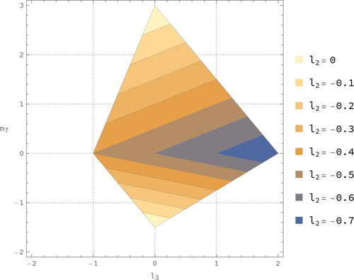
A contour plot of the region defined by Equation (17)(17) $$\begin{array}{cc}\mathrm{ℛ}\hfill & =\{(b,c,d):d\ge 0,\hspace{1em}c-\frac{1}{3}d>-1,\hspace{1em}\frac{5}{3}b+\frac{1}{6}c-\frac{1}{3}d>-1,\hspace{1em}\frac{1}{2}c+\frac{1}{3}d<1\}\hfill \\ \hfill & \hspace{1em}\cup \{(b,c,d):d<0,\hspace{1em}c+\frac{2}{3}d>-1,\hspace{1em}\frac{5}{3}b+\frac{1}{6}c+\frac{2}{3}d>-1,\hspace{1em}\frac{1}{2}c-\frac{2}{3}d<1\}.\hfill \end{array}$$(17) is given in Fig. 1. Note that the conditions given in Equation (17)(17) $$\begin{array}{cc}\mathrm{ℛ}\hfill & =\{(b,c,d):d\ge 0,\hspace{1em}c-\frac{1}{3}d>-1,\hspace{1em}\frac{5}{3}b+\frac{1}{6}c-\frac{1}{3}d>-1,\hspace{1em}\frac{1}{2}c+\frac{1}{3}d<1\}\hfill \\ \hfill & \hspace{1em}\cup \{(b,c,d):d<0,\hspace{1em}c+\frac{2}{3}d>-1,\hspace{1em}\frac{5}{3}b+\frac{1}{6}c+\frac{2}{3}d>-1,\hspace{1em}\frac{1}{2}c-\frac{2}{3}d<1\}.\hfill \end{array}$$(17) reduce to those of Equation (11)(11) $$0<L_1,\mathrm{\hspace{1em}}\mathrm{\hspace{1em}}-\frac{3}{5}<\frac{L_2}{L_1}+\frac{1}{10}\frac{L_3}{L_1},\mathrm{\hspace{1em}}\mathrm{\hspace{1em}}-1<\frac{L_3}{L_1}<2.$$(11) whenever $M_7=0.$

Figure 1. Contour plot of the region $\mathrm{ℛ}$ defined by Equation (17)(17) $$\begin{array}{cc}\mathrm{ℛ}\hfill & =\{(b,c,d):d\ge 0,\hspace{1em}c-\frac{1}{3}d>-1,\hspace{1em}\frac{5}{3}b+\frac{1}{6}c-\frac{1}{3}d>-1,\hspace{1em}\frac{1}{2}c+\frac{1}{3}d<1\}\hfill \\ \hfill & \hspace{1em}\cup \{(b,c,d):d<0,\hspace{1em}c+\frac{2}{3}d>-1,\hspace{1em}\frac{5}{3}b+\frac{1}{6}c+\frac{2}{3}d>-1,\hspace{1em}\frac{1}{2}c-\frac{2}{3}d<1\}.\hfill \end{array}$$(17) in the $({\mathcal{\ell }}_3,m_7)$-plane with ${\mathcal{\ell }}_2=\frac{L_2}{L_1},{\mathcal{\ell }}_3=\frac{L_3}{L_1}$ , and $m_7=\frac{M_7}{L_1}.$ When ${\mathcal{\ell }}_2>0$ the values of ${\mathcal{\ell }}_3$ and m₇ are bounded by the outer large irregular rectangle.

Proof.

From the assumption of Equation (18) and the SO(3) rotation invariance, we have $$-\frac{1}{3} Q_{\alpha \beta ,\gamma }{Q}_{\alpha \beta ,\gamma }\le Q_{\alpha \beta }{Q}_{\mu \nu ,\alpha }{Q}_{\mu \nu ,\beta }\le \frac{2}{3} Q_{\alpha \beta ,\gamma }{Q}_{\alpha \beta ,\gamma }.$$

Then by Theorem 2.1, we know the desired conclusion follows if $L_1>0$ and the tuple $(\frac{L_2}{L_1},\frac{L_3}{L_1},\frac{M_7}{L_1})$ is an element of the set of all $(b,c,d)\in {\mathbb{R}}^3$ such that $$x+\frac{5}{3}b+\frac{1}{6}c>0,\mathrm{\hspace{1em}}\mathrm{\hspace{1em}}x-\frac{1}{2}c>0,\mathrm{\hspace{1em}}\mathrm{\hspace{1em}}x+c>0,$$ where $$x=\{\begin{array}{cc}1-\frac{1}{3}d\hfill & \text{if}\mathrm{ }d\ge 0\hfill \\ 1+\frac{2}{3}d\hfill & \text{if}\mathrm{ }d<0\hfill \end{array}.$$

Elementary algebra shows the latter set is equivalent to the region given by Equation (17)(17) $$\begin{array}{cc}\mathrm{ℛ}\hfill & =\{(b,c,d):d\ge 0,\hspace{1em}c-\frac{1}{3}d>-1,\hspace{1em}\frac{5}{3}b+\frac{1}{6}c-\frac{1}{3}d>-1,\hspace{1em}\frac{1}{2}c+\frac{1}{3}d<1\}\hfill \\ \hfill & \hspace{1em}\cup \{(b,c,d):d<0,\hspace{1em}c+\frac{2}{3}d>-1,\hspace{1em}\frac{5}{3}b+\frac{1}{6}c+\frac{2}{3}d>-1,\hspace{1em}\frac{1}{2}c-\frac{2}{3}d<1\}.\hfill \end{array}$$(17) . □

Remark 2.14.

The work of Ball and Majumdar [24,25] has shown that (for $M_7\ne 0$ and arbitrary boundary conditions) the functional (20) $${\int }_{\Omega }(f_E^{(2)}(\nabla Q)+M_7 Q_{\alpha \beta }{Q}_{\mu \nu ,\alpha }{Q}_{\mu \nu ,\beta }+f_B(Q))dV,$$(20) where the SO(3)-invariant bulk free energy $$f_B(Q)=-a (T-T_c) \text{tr}\mathrm{ }{Q}^2-B \text{tr}\mathrm{ }{Q}^3+C {(\text{tr}\mathrm{ }{Q}^2)}^2,$$ is unbounded below (i.e. there is no global minimizer for the Landau-de Gennes free energy in the form of Equation (20)(20) $${\int }_{\Omega }(f_E^{(2)}(\nabla Q)+M_7 Q_{\alpha \beta }{Q}_{\mu \nu ,\alpha }{Q}_{\mu \nu ,\beta }+f_B(Q))dV,$$(20) when this cubic term is present).

Remark 2.15

(Oseen–Frank’s direction representation). In the constrained uniaxial nematic phase, the director approach to continuum modeling sees rod-like molecules represented by a unit vector $\mathit{n}\in S^2$ in the direction of the principal axis with head-to-tail symmetry. The elastic Oseen–Frank energy is given by $${\int }_{\Omega }W(\mathit{n},\nabla \mathit{n})dV$$ with an integrand of the form (21) $$\begin{array}{c}W(\mathit{n},\nabla \mathit{n})=K_1{(\text{div}\mathrm{ }\mathit{n})}^2+K_2{(\mathit{n}·\text{curl}\mathrm{ }\mathit{n})}^2+K_3|\mathit{n}\times \text{curl}\mathrm{ }\mathit{n}{|}^2\\ \mathrm{\hspace{1em}}\mathrm{\hspace{1em}}+(K_2+K_4)(\text{tr}{(\nabla \mathit{n})}^2-{(\text{div}\mathrm{ }\mathit{n})}^2).\end{array}$$(21)

The first three terms represent energy contributions due to splay, twist, and bend spatial changes of n, respectively; the last term is a null-Lagrangian. The integrand satisfies the invariance properties $$W(\mathit{n},\nabla \mathit{n})=W(-\mathit{n},-\nabla \mathit{n})\hspace{1em}\mathrm{ }\text{and}\mathrm{ }\hspace{1em}W(\mathit{n},\nabla \mathit{n})=W(R\mathit{n},R\nabla \mathit{n}{R}^T)$$ for all $R\in SO(3).$ The first properties account for the lack of polarity of nematics while the second properties express the frame invariance. Experimental measurements of the temperature-dependent elastic constants K₁, K₂, and K₃ are known in various situations (cf. [8,26–29]).

Now in such a uniaxial region, the order tensor elements may be expressed as $$Q=s(\mathit{n}\otimes \mathit{n}-\frac{1}{3}I),$$ where the scalar order parameter s > 0 is required to be constant in the constrained Landau-de Gennes theory. Given this, we find the elastic constants L₁, L₂, L₃, and M₇ for the integrand given by equation (19)(19) $$F(Q,\nabla Q)=f_E^{(2)}(\nabla Q)+M_7 Q_{\alpha \beta }{Q}_{\mu \nu ,\alpha }{Q}_{\mu \nu ,\beta }$$(19) can be related to the above Oseen–Frank elastic constants by the expression (see, e.g. [24,30]) (22) $$\left(\begin{array}{c}{L}_1\\ L_2\\ L_3\\ M_7\end{array}\right)=\frac{1}{s^2}\left(\begin{array}{cccc}\hfill -\frac{1}{6}& \hfill \frac{1}{2}& \hfill \frac{1}{6}& \hfill 0\\ \hfill 1& \hfill -1& \hfill 0& \hfill -1\\ \hfill 0& \hfill 0& \hfill 0& \hfill 1\\ \hfill -\frac{1}{2s}& \hfill 0& \hfill \frac{1}{2s}& \hfill 0\end{array}\right)\left(\begin{array}{c}{K}_1\\ K_2\\ K_3\\ K_4\end{array}\right).$$(22)

It follows that if $L_1>0$ and the tuple $(\frac{L_2}{L_1},\frac{L_3}{L_1},\frac{M_7}{L_1})$ is an element of the region defined by Equation (17)(17) $$\begin{array}{cc}\mathrm{ℛ}\hfill & =\{(b,c,d):d\ge 0,\hspace{1em}c-\frac{1}{3}d>-1,\hspace{1em}\frac{5}{3}b+\frac{1}{6}c-\frac{1}{3}d>-1,\hspace{1em}\frac{1}{2}c+\frac{1}{3}d<1\}\hfill \\ \hfill & \hspace{1em}\cup \{(b,c,d):d<0,\hspace{1em}c+\frac{2}{3}d>-1,\hspace{1em}\frac{5}{3}b+\frac{1}{6}c+\frac{2}{3}d>-1,\hspace{1em}\frac{1}{2}c-\frac{2}{3}d<1\}.\hfill \end{array}$$(17) , i.e. if the integrand $F(Q,\nabla Q)$ given by Equation (19) satisfies the superellipticity of Equation (10)(10) $$f_{P_{\gamma }^{\alpha \beta }{P}_{\rho }^{\mu \nu }}(Q,P){\pi }_{\gamma }^{\alpha \beta }{\pi }_{\rho }^{\mu \nu }\ge l |\pi {|}^2$$(10) , then $K_1>0$ and $(\frac{K_2}{K_1},\frac{K_3}{K_1},\frac{K_4}{K_1})$ is a point in the region $\mathcal{D}\subset {\mathbb{R}}^3,$ where a computation gives (23) $$\begin{array}{c}\mathcal{D}=\{({\kappa }_2,{\kappa }_3,{\kappa }_4):{\kappa }_3\ge 1,(\frac{1}{s}-1\left)\right({\kappa }_3-1)\le 3({\kappa }_2-{\kappa }_4),\\ (\frac{1}{s}-1)({\kappa }_3-1)\le 3({\kappa }_2+2{\kappa }_4),\\ (\frac{1}{s}-1)({\kappa }_3-1)\le 10-7{\kappa }_2-9{\kappa }_4\}\\ \cup \{({\kappa }_2,{\kappa }_3,{\kappa }_4):{\kappa }_3<1,(\frac{2}{s}+1\left)\right(1-{\kappa }_3)\le 3({\kappa }_2-{\kappa }_4),\\ \hspace{0.5em}(\frac{2}{s}+1)(1-{\kappa }_3)\le 3({\kappa }_2+2{\kappa }_4),\\ (\frac{2}{s}+1)(1-{\kappa }_3)\le 10-7{\kappa }_2-9{\kappa }_4\}.\end{array}$$(23)

The conditions for the elastic constants in Equation (23)(23) $$\begin{array}{c}\mathcal{D}=\{({\kappa }_2,{\kappa }_3,{\kappa }_4):{\kappa }_3\ge 1,(\frac{1}{s}-1\left)\right({\kappa }_3-1)\le 3({\kappa }_2-{\kappa }_4),\\ (\frac{1}{s}-1)({\kappa }_3-1)\le 3({\kappa }_2+2{\kappa }_4),\\ (\frac{1}{s}-1)({\kappa }_3-1)\le 10-7{\kappa }_2-9{\kappa }_4\}\\ \cup \{({\kappa }_2,{\kappa }_3,{\kappa }_4):{\kappa }_3<1,(\frac{2}{s}+1\left)\right(1-{\kappa }_3)\le 3({\kappa }_2-{\kappa }_4),\\ \hspace{0.5em}(\frac{2}{s}+1)(1-{\kappa }_3)\le 3({\kappa }_2+2{\kappa }_4),\\ (\frac{2}{s}+1)(1-{\kappa }_3)\le 10-7{\kappa }_2-9{\kappa }_4\}.\end{array}$$(23) are different to the Ericksen inequalities stated in [31]. To get an idea of the admissible parameter space afforded by the conditions in Equation (23(23) $$\begin{array}{c}\mathcal{D}=\{({\kappa }_2,{\kappa }_3,{\kappa }_4):{\kappa }_3\ge 1,(\frac{1}{s}-1\left)\right({\kappa }_3-1)\le 3({\kappa }_2-{\kappa }_4),\\ (\frac{1}{s}-1)({\kappa }_3-1)\le 3({\kappa }_2+2{\kappa }_4),\\ (\frac{1}{s}-1)({\kappa }_3-1)\le 10-7{\kappa }_2-9{\kappa }_4\}\\ \cup \{({\kappa }_2,{\kappa }_3,{\kappa }_4):{\kappa }_3<1,(\frac{2}{s}+1\left)\right(1-{\kappa }_3)\le 3({\kappa }_2-{\kappa }_4),\\ \hspace{0.5em}(\frac{2}{s}+1)(1-{\kappa }_3)\le 3({\kappa }_2+2{\kappa }_4),\\ (\frac{2}{s}+1)(1-{\kappa }_3)\le 10-7{\kappa }_2-9{\kappa }_4\}.\end{array}$$(23) ), a contour plot of the region $\mathcal{D}$ is given for the case $s=\frac{1}{2}$ in Fig. 2.

Figure 2. Contour plots of the region $\mathcal{D}$ defined by Equation (23)(23) $$\begin{array}{c}\mathcal{D}=\{({\kappa }_2,{\kappa }_3,{\kappa }_4):{\kappa }_3\ge 1,(\frac{1}{s}-1\left)\right({\kappa }_3-1)\le 3({\kappa }_2-{\kappa }_4),\\ (\frac{1}{s}-1)({\kappa }_3-1)\le 3({\kappa }_2+2{\kappa }_4),\\ (\frac{1}{s}-1)({\kappa }_3-1)\le 10-7{\kappa }_2-9{\kappa }_4\}\\ \cup \{({\kappa }_2,{\kappa }_3,{\kappa }_4):{\kappa }_3<1,(\frac{2}{s}+1\left)\right(1-{\kappa }_3)\le 3({\kappa }_2-{\kappa }_4),\\ \hspace{0.5em}(\frac{2}{s}+1)(1-{\kappa }_3)\le 3({\kappa }_2+2{\kappa }_4),\\ (\frac{2}{s}+1)(1-{\kappa }_3)\le 10-7{\kappa }_2-9{\kappa }_4\}.\end{array}$$(23) with $s=\frac{1}{2}$ in the $({\kappa }_2,{\kappa }_4)$-plane. The left-hand plot is for the case ${\kappa }_3\le 1$ while the right-hand plot is for the case ${\kappa }_3\ge 1.$

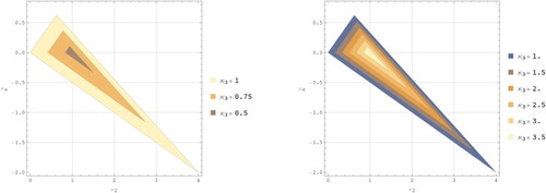
3. Irreducible tensor representations of the rotation group

A Lie algebra is a vector space $\mathfrak{g}$ over a field F together with a Lie bracket (i.e. an alternating bilinear map $\mathfrak{g}\times \mathfrak{g}\to \mathfrak{g}$ denoted $(X,Y)\mapsto [X,Y]$) that satisfies the Jacobi identity $[X,[Y,Z]]+[Y,[Z,X]]+[Z,[X,Y]]=0.$ For a given vector space V, the general linear Lie algebra $\mathfrak{g}\mathfrak{l}(V)$ consists of all linear endomorphisms of V with a Lie bracket given by the commutator of endomorphisms.

A representation $(V,\pi )$ of a Lie algebra $\mathfrak{g}$ comprises a vector space V and a Lie algebra homomorphism $\pi :\mathfrak{g}\to \mathfrak{g}\mathfrak{l}(V).$ This allows one to reproduce the Lie bracket for $\mathfrak{g}$ by the commutator in the general linear algebra of V. The vector space V on which the representation matrices act is called a $\mathfrak{g}$-module; the action $·$ of $\mathfrak{g}$ on V is given by $X·v=\pi (X)v$ for all $X\in \mathfrak{g}$ and $v\in V.$ Conversely, if V is a $\mathfrak{g}$-module then $\pi (X)v=X·v$ defines a representation. Note that it is often convenient to use the language of modules along with the (equivalent) language of representations. A representation $(V,\pi )$ is called irreducible if the only subspaces W of V such that $\pi (X)(W)\subset W$ for all $X\in \mathfrak{g}$ are either {0} or V. If $(V,\pi )$ and $(V\prime ,\pi \prime )$ are two representations of $\mathfrak{g},$ the tensor product representation $\pi \otimes \pi \prime :\mathfrak{g}\to \mathfrak{g}\mathfrak{l}(V\otimes V\prime )$ is defined by $(\pi \otimes \pi \prime )(X)(v\otimes v\prime )=(\pi (X)v)\otimes v\prime +v\otimes (\pi \prime (X)v\prime )$ for all $X\in \mathfrak{g},v\in V$ and $v\prime \in V\prime .$

A representation $(V,\Pi )$ of a Lie group G acting on a finite-dimensional vector space V is a smooth group homomorphism $\Pi :G\to GL(V),$ where GL(V) is the general linear group of all invertible linear transformations of V under their composition. The vector space V on which the representation matrices act is called a G-module; the action $·$ of G on V is given by $g·v=\Pi (g)v$ for all $g\in G$ and $v\in V.$ If $(V,\Pi )$ and $(V\prime ,\Pi \prime )$ are two representations of G, the tensor product representation $\Pi \otimes \Pi \prime :G\to GL(V\otimes V\prime )$ is defined by $(\Pi \otimes \Pi \prime )(g)(v\otimes v\prime )=(\Pi (g)v)\otimes (\Pi (g)v\prime )$ for all $g\in G,v\in V$ and $v\prime \in V\prime .$

A unitary representation $(\mathcal{H},U)$ of a Lie group G acting on a Hilbert space $\mathcal{H}$ over $\mathbb{C}$ is a group homomorphism $U:G\to \text{Isom}(\mathcal{H}),$ where $\text{Isom}(\mathcal{H})$ is the group of unitary operators on the Hilbert space $\mathcal{H}.$ Note that a unitary operator is a bounded linear operator $T:\mathcal{H}\to \mathcal{H}$ which is both surjective and preserves the inner product (in the sense that $〈Tv,Tw〉=〈v,w〉$ for all $v,w\in \mathcal{H}$). The induced linear operator representation $(L(\mathcal{H}),U_1^1)$ acting on the space of linear operators $L(\mathcal{H})$ is given by $U_1^1(g)T=U{(g)}^{-1} T U(g)$ for all $T\in L(\mathcal{H})$ and $g\in G.$

3.1. Relationship between Lie algebra and Lie group representations

We denote by $\mathrm{s}\mathrm{u}(2)$ the real Lie algebra spanned over $\mathbb{R}$ by the set $\{i{L}_x,i{L}_y,i{L}_z\}$ with Lie brackets $$[L_y,L_z]=i{L}_x,\mathrm{\hspace{1em}}\mathrm{\hspace{1em}}[L_z,L_x]=i{L}_y,\mathrm{\hspace{1em}}\mathrm{\hspace{1em}}[L_x,L_y]=i{L}_z.$$

Instead of the generators L_x, L_y it is often more convenient to use the complex combinations $$L_{+}=L_x+i{L}_y\mathrm{\hspace{1em}}\mathrm{\hspace{1em}}\text{and}\mathrm{\hspace{1em}}\mathrm{\hspace{1em}}{L}_{-}=L_x-i{L}_y.$$

We let $\mathrm{s}\mathrm{l}(2;\mathbb{C})$ denote the complex Lie algebra spanned over $\mathbb{C}$ by the set $\{L_{+},L_{-},L_z\}$ with Lie brackets $$[L_z,L_{\pm }]=\pm L_{\pm }\mathrm{\hspace{1em}}\mathrm{\hspace{1em}}\text{and}\mathrm{\hspace{1em}}\mathrm{\hspace{1em}}[L_{+},L_{-}]=2L_z.$$

One then has $\mathrm{s}\mathrm{u}(2)+i \mathrm{s}\mathrm{u}(2)=\mathrm{s}\mathrm{l}(2;\mathbb{C})$ (i.e. the complexified Lie algebra of the former equals the latter).

Theorem 3.1

([20, p. 180]). Let the Lie algebra $\mathfrak{g}$ be either $\mathrm{s}\mathrm{u}(2)$ or its complexification $\mathrm{s}\mathrm{l}(2;\mathbb{C})$. To each spin index $j=0,\frac{1}{2},1,\frac{3}{2},\dots$ there exists an irreducible $(2j+1)$-dimensional representation $(V^j,{\pi }_j)$ of $\mathfrak{g}$. A set of orthonormal basis vectors ${\left\{{\psi }_{j;m}\right\}}_{m=-j}^j$ for the $\mathfrak{g}$-module V^j can be chosen so that $${\pi }_j(L_z){\psi }_{j;m}=m {\psi }_{j;m}$$ $${\pi }_j\left(L_{\pm }\right){\psi }_{j;m}=\sqrt{j(j+1)-m(m\pm 1)} {\psi }_{j;m\pm 1}.$$

Up to equivalence these are the only irreducible representation of $\mathfrak{g}.$

NB: One can think of $L_{+}$ as the ‘creation operator’ or the ‘raising operator’ and $L_{-}$ as the ‘annihilation operator’ or the ‘lowering operator’ (cf. [21, p. 20]).

We now turn to representations of the special orthogonal group $SO(3).$ As the real Lie algebra $\mathrm{s}\mathrm{o}(3)$ of $SO(3)$ (which consists of antisymmetric real 3 × 3 matrices) is in fact isomorphic to $\mathrm{s}\mathrm{u}(2),$ we have:

Corollary 3.2

([20, p. 184], [22, p. 101]). The $(2j+1)$-dimensional irreducible representation of $\mathrm{s}\mathrm{u}(2)$ exponentiates to give a $(2j+1)$-dimensional irreducible representation of SO(3) if and only if $j\in {\mathbb{Z}}_{\ge 0}.$

We remark that since SO(3) is connected, any given finite-dimensional irreducible representation $(V,\Pi )$ of SO(3) implies a unique representation $(V,\pi )$ of $\mathrm{s}\mathrm{o}(3)$ which is also irreducible (cf. [22, p. 79]).

3.2. Tensor products of irreducible representations

If $(V^{j_1},{\pi }_{j_1})$ and $(V^{j_2},{\pi }_{j_2})$ are two irreducible representations of $\mathrm{s}\mathrm{l}(2;\mathbb{C}),$ the decomposition of the tensor product $\mathrm{s}\mathrm{l}(2;\mathbb{C})$-module $V^{j_1}\otimes V^{j_2}$ into irreducible parts has a Clebsch–Gordan series of the form (24) $$V^{j_1}\otimes V^{j_2}=\underset{J=|j_1-j_2|}{\overset{j_1+j_2}{\oplus }}{V}^J$$(24) and is multiplicity free (i.e. V^J appears on the right-hand side only once for $J=|j_1-j_2|,\dots ,j_1+j_2$). We remark that this direct sum is also the Clebsch–Gordan series for $\mathrm{s}\mathrm{u}(2),\mathrm{s}\mathrm{o}(3)$ and SO(3) whenever the spin indices j₁ and j₂ take non-negative integer values (cf. [20, p. 187]).

A natural basis for the tensor product module $V^{j_1}\otimes V^{j_2}$ is given by the tensor product of the orthonormal basis elements, namely ${\psi }_{j_1;m_1}^{(1)}\otimes {\psi }_{j_2;m_2}^{(2)}.$ However, we can also consider a second orthonormal basis $$\{{\psi }_{J;M}={\psi }_{j_1{j}_{2}J;M}:J=|j_1-j_2|,\dots ,j_1+j_2\mathrm{ }\text{and}\mathrm{ }M=-J,\dots ,J\}$$ such that $$\begin{array}{l}({\pi }_{j_1}\otimes {\pi }_{j_2})\left(L_z\right){\psi }_{J;M}=m {\psi }_{J;M}\\ ({\pi }_{j_1}\otimes {\pi }_{j_2})\left(L_{\pm }\right){\psi }_{J;M}=\sqrt{J(J+1)-M(M\pm 1)}{\psi }_{J;M\pm 1}.\end{array}$$

As both $\{{\psi }_{j_1;m_1}^{(1)}\otimes {\psi }_{j_2;m_2}^{(2)}\}$ and $\left\{{\psi }_{J;M}\right\}$ form an orthonormal basis for the tensor product module, there is a unitary transformation between these two sets of bases given by $${\psi }_{J;M}=\sum _{m_1=-j_1}^{j_1}\sum _{m_2=-j_2}^{j_2}〈m_1{m}_2|JM〉{\psi }_{j_1;m_1}^{(1)}\otimes {\psi }_{j_2;m_2}^{(2)}.$$

The coefficients $〈m_1{m}_2|JM〉$ are referred to as the Clebsch–Gordan coefficients, where in the notation $〈m_1{m}_2|JM〉$ we have omitted the numbers j₁ and j₂. When necessary these are included in the form $〈j_1{j}_2{m}_1{m}_2|j_1{j}_{2}JM〉.$

Note that the Clebsch–Gordan coefficients can be expressed in terms of the Wigner 3j-symbols by the formula $$〈m_1{m}_2|JM〉={(-1)}^{j_1-j_2+M}\sqrt{2J+1}\left(\begin{array}{ccc}{j}_1& j_2& J\\ m_1& m_2& -M\end{array}\right)$$ and for J = 0 are given by (25) $$〈m_1{m}_2|0 0〉=\frac{1}{\sqrt{2j_1+1}}{(-1)}^{j_1-m_1}{\delta }_{j_1,j_2}{\delta }_{m_1,-m_2}.$$(25)

The Racah formula gives an explicit, but quite lengthy, general expression for the Clebsch–Gordan coefficients (cf. [21, p. 286], [18, p. 435]).

3.3. Representation theory for a family of linear operators sharing a common invariance group

Let $(V,\Pi )$ be a finite-dimensional representation of a Lie group G on a vector space V and let $\left\{\Pi {(g)}_b^a\right\}$ be its matrix form in a basis ${\left\{e_a\right\}}_{a=1}^{\text{dim}V}$ of the vector space V. Let $(\mathcal{H},U)$ be a unitary representation of a Lie group G acting on a Hilbert space $\mathcal{H}$ with induced linear operator representation $(L(\mathcal{H}),U_1^1).$

An intertwiner between the G-modules V and $L(\mathcal{H})$ is a linear map $\rho :V\to L(\mathcal{H})$ which commutes with the action of G in the sense that $$U_1^1\left(g\right)\circ \rho =\rho \circ \Pi \left(g\right)$$ for all $g\in G,$ i.e. there is a subspace $\rho (V)\subset L(\mathcal{H})$ of operators invariant under conjugation that acts like vectors invariant under the action of $\Pi (g).$ Since ρ is linear, we find that $U{(g)}^{-1} \rho (e_a)U(g)={\sum }_{b=1}^{\dim V}\Pi {(g)}_b^a\rho (e_b)$ for each of the basis vectors e_a of V.

A collection of operators ${\left\{T^a\right\}}_{a=1}^{\dim V}\subset L(\mathcal{H})$ is said to be a tensor operator if it forms such an invariant subspace under an intertwiner $\rho :V\to L(\mathcal{H}),$ i.e. it holds that (26) $$U{(g)}^{-1} T^{a}U(g)=\sum _{b=1}^{\dim V}\Pi {(g)}_b^a{T}^b$$(26) for all $g\in G$ and each $a=1,\dots ,\dim V.$ In other words, a collection of conjugation-invariant operators $\left\{T^a\right\}$ in $L(\mathcal{H})$ transforms like a vector with respect to the group action on the G-module V. When the representation Π is irreducible, $\left\{T^a\right\}$ is said to be an irreducible tensor operator (cf. [19, Chapter 9]). Note that any intertwiner between two irreducible G-modules is either an isomorphism or zero by Schur’s lemma.

The corresponding definition of tensor operators on the level of the Lie algebra $\mathfrak{g}$ of the Lie group G is obtained by inserting the representation of the infinitesimal generators (cf. [22, p. 79]) $$\pi (X)=\frac{d}{dt}\Pi (\hspace{0.17em}\text{exp}\hspace{0.17em}tX){|}_{t=0}\mathrm{\hspace{1em}}\mathrm{\hspace{1em}}\text{and}\mathrm{\hspace{1em}}\mathrm{\hspace{1em}}u(X)=-i\frac{d}{dt}U(\hspace{0.17em}\text{exp}\hspace{0.17em}tX){|}_{t=0}$$ into Equation (26)(26) $$U{(g)}^{-1} T^{a}U(g)=\sum _{b=1}^{\dim V}\Pi {(g)}_b^a{T}^b$$(26) to obtain (27) $$[u(X),T^a]=i\sum _{b=1}^{\dim V}\pi {(X)}_b^a{T}^b$$(27) for all $X\in \mathfrak{g}$ and each $a=1,\dots ,\dim V.$ Note that $\pi :\mathfrak{g}\to \mathfrak{g}\mathfrak{l}(V)$ is the induced representation of $\mathfrak{g}$ on the vector space V and that $u:\mathfrak{g}\to \mathrm{i}\mathrm{s}\mathrm{o}\mathrm{m}(\mathcal{H})$ is the induced unitary representation of $\mathrm{g}$ on the Hilbert space $\mathcal{H}$ (where $\mathrm{i}\mathrm{s}\mathrm{o}\mathrm{m}(\mathcal{H})$ is Lie algebra of anti-Hermitian operators).

Both definition, Equations (26(26) $$U{(g)}^{-1} T^{a}U(g)=\sum _{b=1}^{\dim V}\Pi {(g)}_b^a{T}^b$$(26) ) and (27(27) $$[u(X),T^a]=i\sum _{b=1}^{\dim V}\pi {(X)}_b^a{T}^b$$(27) ) are equivalent whenever the Lie exponential map $\text{exp}\hspace{0.17em}:\mathfrak{g}\to G$ is surjective. In particular, the exponential map of a compact connected Lie group is surjective (cf. [21, p. 149]). Moreover, SO(3) is both compact and connected.

3.4. Spherical tensors

For a $(2j+1)$-dimensional irreducible representation $(V^j,{\Pi }_j)$ of the rotation group SO(3) with $j\in {\mathbb{Z}}_{\ge 0},$ the set of $2j+1$ components of an irreducible tensor operator must satisfy the rotation condition of Equation (26)(26) $$U{(g)}^{-1} T^{a}U(g)=\sum _{b=1}^{\dim V}\Pi {(g)}_b^a{T}^b$$(26) . A set of such quantities, denoted by ${\mathit{T}}_j={\left\{T_{j;m}\right\}}_{m=-j}^j\subset L(\mathcal{H}),$ is called a spherical tensor of degree j (cf. [18,32]). For any $R\in SO(3),$ the components satisfy the condition $$U{(R)}^{-1}{T}_{j;m}U(R)=\sum _{m\prime =-j}^j{\Pi }_j{(R)}_m^{m\prime }{T}_{j;m\prime }$$ where the coefficients ${\Pi }_j{(R)}_m^{m\prime }$ form a matrix of order $2j+1$ with respect to m and $m\prime .$ Each $T_{j;m}$ is equivalent, as regards their transformation properties, to a set of $2j+1$ spherical harmonic functions Y_jm (here the spherical harmonics play the role of operators and not of eigenfunctions). A computation (cf. [23, p. 55]) involving infinitesimal rotations for Equation (26)(26) $$U{(g)}^{-1} T^{a}U(g)=\sum _{b=1}^{\dim V}\Pi {(g)}_b^a{T}^b$$(26) yields the Racah commutative relations $$\begin{array}{l}\left[u\right(L_{\pm }),T_{j;m}]=\sqrt{j(j+1)-m(m\pm 1)} T_{j;m\pm 1}\\ \left[u\right(L_z),T_{j;m}]=m T_{j;m}.\end{array}$$

The construction of tensor products of spherical tensors $S_{j_1;m_1}$ and $T_{j_2;m_2}$ follows the above decomposition of Section 3.2, i.e. one can form spherical tensors of degrees $J=|j_1-j_2|,\dots ,j_1+j_2$ by means of the formulae (28) $${({\mathit{S}}_{j_1}\otimes {\mathit{T}}_{j_2})}_{J;M}=\sum _{m_1,m_2}〈m_1{m}_2|JM〉S_{j_1;m_1}{T}_{j_2;m_2}.$$(28)

Such tensor products satisfy the condition of Equation (26)(26) $$U{(g)}^{-1} T^{a}U(g)=\sum _{b=1}^{\dim V}\Pi {(g)}_b^a{T}^b$$(26) . The scalar product of spherical tensors of the same degree j is given by (29) $${({\mathit{S}}_j\otimes {\mathit{T}}_j)}_{0;0}=\frac{1}{\sqrt{2j+1}}\sum _m{S}_{j;m}{T}_{j;m}{}^{*}$$(29) where the complex conjugate of a spherical tensor is given by $$T_{j;m}{}^{*}={(-1)}^{j-m}{T}_{j;-m}.$$

3.5. Transformation between Cartesian and spherical tensors

It is desirable to relate the components $T_{{\alpha }_1\cdots {\alpha }_n}$ of a Cartesian tensor of rank n to their spherical counterparts $T_{j_1\cdots j_n;m}$ of degree j_n, i.e. by a general transformation law of the form $$T_{j_1\cdots j_n;m}=\sum _{{\alpha }_1\cdots {\alpha }_n}{T}_{{\alpha }_1\cdots {\alpha }_n}〈{\alpha }_1\cdots {\alpha }_n|j_1\cdots j_n;m〉$$ and, conversely, $$T_{{\alpha }_1\cdots {\alpha }_n}=\sum _{j_1\cdots j_n;m}{T}_{j_1\cdots j_n;m}〈j_1\cdots j_n;m|{\alpha }_1\cdots {\alpha }_n〉$$ with the unitary condition $〈{\alpha }_1\cdots {\alpha }_n|j_1\cdots j_n;m〉={〈j_1\cdots j_n;m|{\alpha }_1\cdots {\alpha }_n〉}^{*}.$ Note that the subscripts j₁, j₂, …, $j_{n-1}$ are sometimes required to distinguish between different spherical tensors with the same degree j_n; they can often be dropped all together where no ambiguity results. In particular, j₁ is always one but is included in the notation for completeness.

For low-rank tensors of n = 0 (scalars) or n = 1 (vectors), the transformation to spherical tensors is straightforward and unambiguous since the tensors are already irreducible. In the case of scalars the transformation is the identity $T_{0;0}=T〈|;0〉=T.$ Vector quantities can be expressed either in a Cartesian basis $|\alpha 〉$ with directions $\alpha =x,y,z$ or in a spherical basis $|1;m〉$ with $m=-1,0,1.$ The unitary transformation $〈\alpha |1;m〉$ between bases is given by $$\begin{array}{c}\begin{array}{ccccc}\hfill & \hfill & |1;1〉\hfill & |1;0〉\hfill & |1;-1〉\hfill \end{array}\\ \begin{array}{c}〈x|\hfill \\ 〈y|\hfill \\ 〈z|\hfill \end{array}\left(\begin{array}{ccccc}-\frac{i}{\sqrt{2}}& \hfill & 0& \hfill & \frac{i}{\sqrt{2}}\\ \frac{1}{\sqrt{2}}& \hfill & 0& \hfill & \frac{1}{\sqrt{2}}\\ 0& \hfill & i& \hfill & 0\end{array}\right)\end{array}$$ or equivalently $$T_{1;\pm 1}=\mp \frac{i}{\sqrt{2}}(T_x\pm i T_y)\mathrm{\hspace{1em}}\mathrm{\hspace{1em}}\text{and}\mathrm{\hspace{1em}}\mathrm{\hspace{1em}}{T}_{1;0}=i T_z.$$

Note that a direct computation shows $${({\mathit{S}}_1\otimes {\mathit{T}}_1)}_{0;0}=\frac{1}{\sqrt{3}}(S_x{T}_x+S_y{T}_y+S_z{T}_z),$$ i.e. the Euclidean dot product of vectors is, up to a constant, equal to the scalar product of spherical tensors of degree $j_1=1$ (cf. Equation (29)(29) $${({\mathit{S}}_j\otimes {\mathit{T}}_j)}_{0;0}=\frac{1}{\sqrt{2j+1}}\sum _m{S}_{j;m}{T}_{j;m}{}^{*}$$(29) ).

For higher-order tensors, the transformation coefficients can be calculated recursively (cf. [33,34]) by the relation $$\begin{array}{c}〈{\alpha }_1\cdots {\alpha }_n|j_1\cdots j_n;m〉\\ \mathrm{\hspace{1em}}=\sum _{m\prime ,m″}〈{\alpha }_1\cdots {\alpha }_{n-1}|j_1\cdots j_{n-1};m\prime 〉〈{\alpha }_n|1;m″〉〈j_{n-1}1m\prime m″|j_{n-1}1j_{n}m〉,\end{array}$$ where $〈j_{n-1}1m\prime m″|j_{n-1}1j_{n}m〉$ are the Clebsch–Gordan coefficients. In particular, the transformation coefficients for n = 2 are given by $$\begin{array}{c}\begin{array}{ccccccccc}\hfill & \hfill & \hfill & |10;0〉\hfill & |11;0〉\hfill & |11;1〉\hfill & |12;0〉\hfill & |12;1〉\hfill & |12;2〉\hfill \end{array}\\ \begin{array}{c}〈xx|\hfill \\ 〈xy|\hfill \\ 〈xz|\hfill \\ 〈yx|\hfill \\ 〈yy|\hfill \\ 〈yz|\hfill \\ 〈zx|\hfill \\ 〈zy|\hfill \\ 〈zz|\hfill \end{array}\left(\begin{array}{ccccccccccc}\frac{1}{\sqrt{3}}\hfill & \hfill & 0\hfill & \hfill & 0\hfill & \hfill & \frac{1}{\sqrt{6}}\hfill & \hfill & 0\hfill & \hfill & -\frac{1}{2}\hfill \\ 0\hfill & \hfill & -\frac{i}{\sqrt{2}}\hfill & \hfill & 0\hfill & \hfill & 0\hfill & \hfill & 0\hfill & \hfill & -\frac{i}{2}\hfill \\ 0\hfill & \hfill & 0\hfill & \hfill & \frac{1}{2}\hfill & \hfill & 0\hfill & \hfill & \frac{1}{2}\hfill & \hfill & 0\hfill \\ 0\hfill & \hfill & \frac{i}{\sqrt{2}}\hfill & \hfill & 0\hfill & \hfill & 0\hfill & \hfill & 0\hfill & \hfill & -\frac{i}{2}\hfill \\ \frac{1}{\sqrt{3}}\hfill & \hfill & 0\hfill & \hfill & 0\hfill & \hfill & \frac{1}{\sqrt{6}}\hfill & \hfill & 0\hfill & \hfill & \frac{1}{2}\hfill \\ 0\hfill & \hfill & 0\hfill & \hfill & \frac{i}{2}\hfill & \hfill & 0\hfill & \hfill & \frac{i}{2}\hfill & \hfill & 0\hfill \\ 0\hfill & \hfill & 0\hfill & \hfill & -\frac{1}{2}\hfill & \hfill & 0\hfill & \hfill & \frac{1}{2}\hfill & \hfill & 0\hfill \\ 0\hfill & \hfill & 0\hfill & \hfill & -\frac{i}{2}\hfill & \hfill & 0\hfill & \hfill & \frac{i}{2}\hfill & \hfill & 0\hfill \\ \frac{1}{\sqrt{3}}\hfill & \hfill & 0\hfill & \hfill & 0\hfill & \hfill & -\frac{\sqrt{2}}{\sqrt{3}}\hfill & \hfill & \hfill & 0\hfill & 0\hfill \end{array}\right)\end{array}$$ i.e. the components of a spherical tensor of degrees $j_2=0,1,2$ are given in terms of the Cartesian tensor components T_αβ by the formulae: (30) $$\begin{array}{l}{T}_{0;0}=\frac{T_{xx}+T_{yy}+T_{zz}}{\sqrt{3}}\\ T_{1;0}=-\frac{i\left(T_{xy}-T_{yx}\right)}{\sqrt{2}}\\ T_{1;\pm 1}=\frac{1}{2}\left(T_{xz}-T_{zx}\pm i\left(T_{yz}-T_{zy}\right)\right)\end{array}\mathrm{\hspace{1em}}\mathrm{\hspace{1em}}\begin{array}{l}{T}_{2;0}=\frac{T_{xx}+T_{yy}-2 T_{zz}}{\sqrt{6}}\\ T_{2;\pm 1}=\pm \frac{1}{2}\left(T_{xz}+T_{zx}\pm i (T_{yz}+T_{zy})\right)\\ T_{2;\pm 2}=-\frac{1}{2}\left(T_{xx}-T_{yy}\pm i (T_{xy}+T_{yx})\right)\end{array}$$(30)

Note that this corresponds to the decomposition of 2-tensors into the direct sum of SO(3)-invariant subspaces represented by the trace ${\mathit{T}}_0,$ the antisymmetric matrices ${\mathit{T}}_1$ and the traceless symmetric matrices ${\mathit{T}}_2.$ In fact, for the scalar product of spherical tensors of degree 2, we have $${({\mathit{S}}_2\otimes {\mathit{T}}_2)}_{0;0}=\frac{1}{\sqrt{5}}\sum _{\alpha ,\beta }{S}_{\alpha \beta }{T}_{\alpha \beta }$$ whenever the Cartesian tensors S_αβ and T_αβ of rank two are symmetric and traceless.

4. Transformation between Cartesian and spherical representations of SO(3)-invariant integrand expansions

As the space of symmetric traceless 2-tensors forms an irreducible subspace under the action of SO(3) by conjugation, the spherical components of the 2-tensor’s Cartesian components Q_αβ ($\alpha =x,y,z$) form a quadrupole tensor ${\mathit{Q}}_2$ (i.e. a spherical tensor of degree 2). From Equation (30)(30) $$\begin{array}{l}{T}_{0;0}=\frac{T_{xx}+T_{yy}+T_{zz}}{\sqrt{3}}\\ T_{1;0}=-\frac{i\left(T_{xy}-T_{yx}\right)}{\sqrt{2}}\\ T_{1;\pm 1}=\frac{1}{2}\left(T_{xz}-T_{zx}\pm i\left(T_{yz}-T_{zy}\right)\right)\end{array}\mathrm{\hspace{1em}}\mathrm{\hspace{1em}}\begin{array}{l}{T}_{2;0}=\frac{T_{xx}+T_{yy}-2 T_{zz}}{\sqrt{6}}\\ T_{2;\pm 1}=\pm \frac{1}{2}\left(T_{xz}+T_{zx}\pm i (T_{yz}+T_{zy})\right)\\ T_{2;\pm 2}=-\frac{1}{2}\left(T_{xx}-T_{yy}\pm i (T_{xy}+T_{yx})\right)\end{array}$$(30) the spherical tensor’s components $Q_{2;m}$ ($m=0,\pm 1,\pm 2$) are given by (31) $$\begin{array}{cc}{Q}_{2;\pm 2}\hfill & =-\frac{1}{2}(Q_{xx}-Q_{yy}\pm 2i Q_{xy})\hfill \\ Q_{2;\pm 1}\hfill & =\pm (Q_{xz}\pm i Q_{yz})\hfill \\ Q_{2;0}\hfill & =-\frac{\sqrt{3}}{\sqrt{2}}{Q}_{zz}\hfill \end{array}$$(31) with $Q_{xx}+Q_{yy}+Q_{zz}=0.$ The spherical components of the vector operator ${\partial }_{\alpha }=\frac{\partial }{\partial x_{\alpha }}$ ($\alpha =x,y,z$) forms a dipole vector operator ${\partial }_1$ (i.e. a spherical tensor of degree 1) with components ${\partial }_{1;m}$ ($m=0,\pm 1$) given by (32) $$\begin{array}{cc}{\partial }_{1;\pm 1}\hfill & =\mp \frac{i}{\sqrt{2}}({\partial }_x\pm i {\partial }_y)\hfill \\ {\partial }_{1;0}\hfill & =i {\partial }_z.\hfill \end{array}$$(32)

The action of the dipole vector operator ${\partial }_1$ on the quadrupole tensor ${\mathit{Q}}_2$ is given by the tensor product ${\partial }_1\otimes {\mathit{Q}}_2.$ The decomposition of this tensor product (cf. the spherical tensor product formula of Equation (28)(28) $${({\mathit{S}}_{j_1}\otimes {\mathit{T}}_{j_2})}_{J;M}=\sum _{m_1,m_2}〈m_1{m}_2|JM〉S_{j_1;m_1}{T}_{j_2;m_2}.$$(28) ) yields spherical tensors ${({\partial }_1\otimes {\mathit{Q}}_2)}_L$ of degrees L = 1, 2, three with components given by the formula (33) $${({\partial }_1\otimes {\mathit{Q}}_2)}_{L;M}=\sum _{m_1=-1}^1\sum _{m_2=-2}^2〈m_1{m}_2|LM〉 {\partial }_{1;m_1}{Q}_{2;m_2}.$$(33)

Our objective is to rewrite these spherical tensor components in terms of $Q_{\alpha \beta ,\gamma }$ (i.e. the partial derivatives of the Q-tensor in the original Cartesian coordinates). In order to do so, we introduce the notational abbreviation (34) $$Q_{m_2,m_1}={\partial }_{1;m_1}{Q}_{2;m_2}$$(34) with $m_1=-1,0,1$ and $m_2=-2,-1,0,1,2.$ Then, by plugging the Equations (32(32) $$\begin{array}{cc}{\partial }_{1;\pm 1}\hfill & =\mp \frac{i}{\sqrt{2}}({\partial }_x\pm i {\partial }_y)\hfill \\ {\partial }_{1;0}\hfill & =i {\partial }_z.\hfill \end{array}$$(32) ) and (31(31) $$\begin{array}{cc}{Q}_{2;\pm 2}\hfill & =-\frac{1}{2}(Q_{xx}-Q_{yy}\pm 2i Q_{xy})\hfill \\ Q_{2;\pm 1}\hfill & =\pm (Q_{xz}\pm i Q_{yz})\hfill \\ Q_{2;0}\hfill & =-\frac{\sqrt{3}}{\sqrt{2}}{Q}_{zz}\hfill \end{array}$$(31) ) into the right-hand side of Equation (34)(34) $$Q_{m_2,m_1}={\partial }_{1;m_1}{Q}_{2;m_2}$$(34) , a computation (cf. Appendix B.1) shows that the components $Q_{m_2,m_1}$ are given in terms of their Cartesian derivatives $Q_{\alpha \beta ,\gamma }$ by the expressions: (35a) $$\begin{array}{c}\begin{array}{c}{Q}_{\pm 2,-1}=\frac{1}{2\sqrt{2}}(-i Q_{xx,x}\pm 2 Q_{xy,x}+i Q_{yy,x}-Q_{xx,y}\mp 2i Q_{xy,y}+Q_{yy,y})\hfill \\ Q_{\pm 2,0}=-\frac{i}{2}{Q}_{xx,z}\pm Q_{xy,z}+\frac{i}{2}{Q}_{yy,z}\hfill \\ Q_{\pm 2,1}=\frac{1}{2\sqrt{2}}(i Q_{xx,x}\mp 2 Q_{xy,x}-i Q_{yy,x}-Q_{xx,y}\mp 2i Q_{xy,y}+Q_{yy,y})\hfill \end{array}\}\end{array}$$(35a) (35b) $$\begin{array}{c}\begin{array}{c}{Q}_{\pm 1,-1}=\frac{1}{\sqrt{2}}(\pm i Q_{xz,x}-Q_{yz,x}\pm Q_{xz,y}+i Q_{yz,y})\hfill \\ Q_{\pm 1,0}=-Q_{yz,z}\pm i Q_{xz,z}\hfill \\ Q_{\pm 1,1}=\frac{1}{\sqrt{2}}(\mp i Q_{xz,x}+Q_{yz,x}\pm Q_{xz,y}+i Q_{yz,y})\hfill \end{array}\}\end{array}$$(35b) (35c) $$\begin{array}{c}\begin{array}{c}{Q}_{0,-1}=\frac{\sqrt{3}}{2}\left(i Q_{xx,x}+i Q_{yy,x}+Q_{xx,y}+Q_{yy,y}\right)\hfill \\ Q_{0,0}=i\frac{\sqrt{3}}{\sqrt{2}}\left(Q_{xx,z}+Q_{yy,z}\right)\hfill \\ Q_{0,1}=\frac{\sqrt{3}}{2}\left(-i Q_{xx,x}-i Q_{yy,x}+Q_{xx,y}+Q_{yy,y}\right)\hfill \end{array}\}\end{array}$$(35c)

We now look to proving the results from Section 2 by exploiting the above relationships between Cartesian and spherical tensor representations.

4.1. Proof of Theorem 2.1

We exploit the fact that spherical tensor representations offer linearly independent invariants of the Q-tensor partial derivatives. Indeed, the scalar products given by Equation (29)(29) $${({\mathit{S}}_j\otimes {\mathit{T}}_j)}_{0;0}=\frac{1}{\sqrt{2j+1}}\sum _m{S}_{j;m}{T}_{j;m}{}^{*}$$(29) of the spherical tensors ${({\partial }_1\otimes {\mathit{Q}}_2)}_L$ yield invariants of the form (36) $$\begin{array}{c}{\mathrm{ℐ}}^{\left(2\right)}\left(L\right)={({({\partial }_1\otimes {\mathit{Q}}_2)}_L\otimes {({\partial }_1\otimes {\mathit{Q}}_2)}_L)}_{0;0}\\ =\frac{1}{\sqrt{2L+1}}\sum _{m=-L}^L{(-1)}^{L-m}{({\partial }_1\otimes {\mathit{Q}}_2)}_{L;m}{({\partial }_1\otimes {\mathit{Q}}_2)}_{L;-m}.\end{array}$$(36)

By Equation (25(25) $$〈m_1{m}_2|0 0〉=\frac{1}{\sqrt{2j_1+1}}{(-1)}^{j_1-m_1}{\delta }_{j_1,j_2}{\delta }_{m_1,-m_2}.$$(25) ), the spherical tensors ${({\partial }_1\otimes {\mathit{Q}}_2)}_L$ also have the orthogonality property $${({({\partial }_1\otimes {\mathit{Q}}_2)}_L\otimes {({\partial }_1\otimes {\mathit{Q}}_2)}_{L\prime })}_{0;0}=0\hspace{1em}\mathrm{ }\text{whenever}\mathrm{ }\hspace{1em}L\ne L\prime .$$

Therefore, by rewriting expansion given by Equation (1(1) $$f_E^{(2)}(\nabla Q)=L_1 Q_{\alpha \beta ,\gamma }{Q}_{\alpha \beta ,\gamma }+L_2 Q_{\alpha \beta ,\beta }{Q}_{\alpha \gamma ,\gamma }+L_3 Q_{\alpha \beta ,\gamma }{Q}_{\alpha \gamma ,\beta }$$(1) ) as a linear combination of these invariants, i.e. by writing (37) $$f_E^{(2)}(\nabla Q)=\sum _{L=1}^3{\Lambda }_L {\mathrm{ℐ}}^{(2)}(L),$$(37) the superelliptic condition of Equation (10)(10) $$f_{P_{\gamma }^{\alpha \beta }{P}_{\rho }^{\mu \nu }}(Q,P){\pi }_{\gamma }^{\alpha \beta }{\pi }_{\rho }^{\mu \nu }\ge l |\pi {|}^2$$(10) is fulfilled whenever the constants ${\Lambda }_1,{\Lambda }_2,$ and ${\Lambda }_3$ are positive (since the invariants ${\mathrm{ℐ}}^{(2)}(L)\ge 0$ by the scalar product of Equation (29(29) $${({\mathit{S}}_j\otimes {\mathit{T}}_j)}_{0;0}=\frac{1}{\sqrt{2j+1}}\sum _m{S}_{j;m}{T}_{j;m}{}^{*}$$(29) )). All that remains is to relate the ${\Lambda }_1,{\Lambda }_2,{\Lambda }_3$ constants to the original L₁, L₂, and L₃ elliptic constants given in Equation (1)(1) $$f_E^{(2)}(\nabla Q)=L_1 Q_{\alpha \beta ,\gamma }{Q}_{\alpha \beta ,\gamma }+L_2 Q_{\alpha \beta ,\beta }{Q}_{\alpha \gamma ,\gamma }+L_3 Q_{\alpha \beta ,\gamma }{Q}_{\alpha \gamma ,\beta }$$(1) .

For the Cartesian expansion of Equation (1)(1) $$f_E^{(2)}(\nabla Q)=L_1 Q_{\alpha \beta ,\gamma }{Q}_{\alpha \beta ,\gamma }+L_2 Q_{\alpha \beta ,\beta }{Q}_{\alpha \gamma ,\gamma }+L_3 Q_{\alpha \beta ,\gamma }{Q}_{\alpha \gamma ,\beta }$$(1) , we need to take into account the Q-tensor symmetry conditions, namely the traceless condition $\text{tr}\mathrm{ }Q=0$ and the symmetric condition $Q_{\alpha \beta }=Q_{\beta \alpha }$ (which implies that $Q_{\alpha \beta ,\gamma }=Q_{\beta \alpha ,\gamma }$). Due to the symmetry requirements, we want to identify the lower triangle matrix elements of Q with the upper triangle matrix elements, i.e. we want to set Q_yx = Q_xy, Q_zx = Q_xz and Q_zy = Q_yz wherever this occurs. Furthermore, from the traceless condition, we want to also set $Q_{zz}=-Q_{xx}-Q_{yy}$ whenever this occurs. In which case the Cartesian expression of Equation (1)(1) $$f_E^{(2)}(\nabla Q)=L_1 Q_{\alpha \beta ,\gamma }{Q}_{\alpha \beta ,\gamma }+L_2 Q_{\alpha \beta ,\beta }{Q}_{\alpha \gamma ,\gamma }+L_3 Q_{\alpha \beta ,\gamma }{Q}_{\alpha \gamma ,\beta }$$(1) can be considered as a quadratic polynomial in the variables (38) $$\begin{array}{cc}\hfill & Q_{xx,x},\hspace{1em}{Q}_{xx,y},\hspace{1em}{Q}_{xx,z},\hfill \\ \hfill & Q_{yy,x},\hspace{1em}{Q}_{yy,y},\hspace{1em}{Q}_{yy,z},\hfill \\ \hfill & Q_{xy,x},\hspace{1em}{Q}_{xy,y},\hspace{1em}{Q}_{xy,z},\hfill \\ \hfill & Q_{xz,x},\hspace{1em}{Q}_{xz,y},\hspace{1em}{Q}_{xz,z},\hfill \\ \hfill & Q_{yz,x},\hspace{1em}{Q}_{yz,y},\hspace{1em}{Q}_{yz,z}.\hfill \end{array}$$(38)

Indeed, a direct computation (cf. exprL2 in Appendix C.1) shows that the explicit expansion of Equation (1)(1) $$f_E^{(2)}(\nabla Q)=L_1 Q_{\alpha \beta ,\gamma }{Q}_{\alpha \beta ,\gamma }+L_2 Q_{\alpha \beta ,\beta }{Q}_{\alpha \gamma ,\gamma }+L_3 Q_{\alpha \beta ,\gamma }{Q}_{\alpha \gamma ,\beta }$$(1) as a polynomial in the variables in Equation (38)(38) $$\begin{array}{cc}\hfill & Q_{xx,x},\hspace{1em}{Q}_{xx,y},\hspace{1em}{Q}_{xx,z},\hfill \\ \hfill & Q_{yy,x},\hspace{1em}{Q}_{yy,y},\hspace{1em}{Q}_{yy,z},\hfill \\ \hfill & Q_{xy,x},\hspace{1em}{Q}_{xy,y},\hspace{1em}{Q}_{xy,z},\hfill \\ \hfill & Q_{xz,x},\hspace{1em}{Q}_{xz,y},\hspace{1em}{Q}_{xz,z},\hfill \\ \hfill & Q_{yz,x},\hspace{1em}{Q}_{yz,y},\hspace{1em}{Q}_{yz,z}.\hfill \end{array}$$(38) takes the form (39) $$\begin{array}{l}{f}_E^{\left(2\right)}(\nabla Q)=2L_1[Q_{xx,y}^2+Q_{xy,z}^2+Q_{xz,y}^2+Q_{yy,x}^2+Q_{yz,x}^2+Q_{xx,y}{Q}_{yy,y}+Q_{xx,x}{Q}_{yy,x}]\\ +2L_2[Q_{xx,x}{Q}_{xy,y}+Q_{xy,x}{Q}_{yy,y}+Q_{xy,x}{Q}_{yz,z}+Q_{xy,y}{Q}_{xz,z}+Q_{xz,x}{Q}_{yz,y}\\ -Q_{xx,z}{Q}_{yz,y}-Q_{xz,x}{Q}_{yy,z}]\\ +2L_3[Q_{xy,x}{Q}_{xx,y}+Q_{xy,z}{Q}_{xz,y}+Q_{yy,x}{Q}_{xy,y}+Q_{yz,x}{Q}_{xz,y}+Q_{yz,x}{Q}_{xy,z}\\ -Q_{xx,y}{Q}_{yz,z}-Q_{yy,x}{Q}_{xz,z}]\\ +(2L_1+L_2+L_3)[Q_{xx,x}^2+Q_{xx,z}^2+Q_{xy,x}^2+Q_{xy,y}^2+Q_{xz,x}^2+Q_{xz,z}^2\\ +Q_{yy,y}^2+Q_{yy,z}^2+Q_{yz,y}^2+Q_{yz,z}^2]\\ +2(L_1+L_2+L_3)Q_{xx,z}{Q}_{yy,z}\\ +2(L_2-L_3)[Q_{xx,x}{Q}_{xz,z}+Q_{yy,y}{Q}_{yz,z}-Q_{xx,z}{Q}_{xz,x}-Q_{yy,z}{Q}_{yz,y}].\end{array}$$(39)

On the other hand, one can expand the right-hand side of Equation (37)(37) $$f_E^{(2)}(\nabla Q)=\sum _{L=1}^3{\Lambda }_L {\mathrm{ℐ}}^{(2)}(L),$$(37) by way of the spherical tensor product formula of Equation (33(33) $${({\partial }_1\otimes {\mathit{Q}}_2)}_{L;M}=\sum _{m_1=-1}^1\sum _{m_2=-2}^2〈m_1{m}_2|LM〉 {\partial }_{1;m_1}{Q}_{2;m_2}.$$(33) ). This gives Equation (37)(37) $$f_E^{(2)}(\nabla Q)=\sum _{L=1}^3{\Lambda }_L {\mathrm{ℐ}}^{(2)}(L),$$(37) as a quadratic polynomial in the variables given by Equation (34)(34) $$Q_{m_2,m_1}={\partial }_{1;m_1}{Q}_{2;m_2}$$(34) . Then by making the substitutions of Equation (35), a computation (cf. exprK2 in Appendix C.1) shows that the spherical tensor expansion in Equation (37)(37) $$f_E^{(2)}(\nabla Q)=\sum _{L=1}^3{\Lambda }_L {\mathrm{ℐ}}^{(2)}(L),$$(37) – rewritten in terms of the Cartesian variables in Equation (38)(38) $$\begin{array}{cc}\hfill & Q_{xx,x},\hspace{1em}{Q}_{xx,y},\hspace{1em}{Q}_{xx,z},\hfill \\ \hfill & Q_{yy,x},\hspace{1em}{Q}_{yy,y},\hspace{1em}{Q}_{yy,z},\hfill \\ \hfill & Q_{xy,x},\hspace{1em}{Q}_{xy,y},\hspace{1em}{Q}_{xy,z},\hfill \\ \hfill & Q_{xz,x},\hspace{1em}{Q}_{xz,y},\hspace{1em}{Q}_{xz,z},\hfill \\ \hfill & Q_{yz,x},\hspace{1em}{Q}_{yz,y},\hspace{1em}{Q}_{yz,z}.\hfill \end{array}$$(38) – takes the form (40) $$\begin{array}{l}{f}_E^{\left(2\right)}(\nabla Q)=(\frac{4}{3\sqrt{5}}{\Lambda }_2+\frac{2}{3\sqrt{7}}{\Lambda }_3)[Q_{xx,y}^2+Q_{xy,z}^2+Q_{xz,y}^2+Q_{yy,x}^2+Q_{yz,x}^2\\ \mathrm{\hspace{1em}}\mathrm{\hspace{1em}}+Q_{xx,y}{Q}_{yy,y}+Q_{xx,x}{Q}_{yy,x}]\\ +(\frac{2\sqrt{3}}{5}{\Lambda }_1-\frac{2}{3\sqrt{5}}{\Lambda }_2-\frac{8}{15\sqrt{7}}{\Lambda }_3)[Q_{xx,x}{Q}_{xy,y}+Q_{xy,x}{Q}_{yy,y}+Q_{xy,x}{Q}_{yz,z}\\ \mathrm{\hspace{1em}}\mathrm{\hspace{1em}}+Q_{xy,y}{Q}_{xz,z}+Q_{xz,x}{Q}_{yz,y}\\ \mathrm{\hspace{1em}}\mathrm{\hspace{1em}}-Q_{xx,z}{Q}_{yz,y}-Q_{xz,x}{Q}_{yy,z}]\\ +(-\frac{4}{3\sqrt{5}}{\Lambda }_2+\frac{4}{3\sqrt{7}}{\Lambda }_3)[Q_{xy,x}{Q}_{xx,y}+Q_{xy,z}{Q}_{xz,y}+Q_{yy,x}{Q}_{xy,y}\\ \mathrm{\hspace{1em}}\mathrm{\hspace{1em}}+Q_{yz,x}{Q}_{xz,y}+Q_{yz,x}{Q}_{xy,z}\\ \mathrm{\hspace{1em}}\mathrm{\hspace{1em}}-Q_{xx,y}{Q}_{yz,z}-Q_{yy,x}{Q}_{xz,z}]\\ +(\frac{\sqrt{3}}{5}{\Lambda }_1+\frac{1}{3\sqrt{5}}{\Lambda }_2+\frac{16}{15\sqrt{7}}{\Lambda }_3)[Q_{xx,x}^2+Q_{xx,z}^2+Q_{xy,x}^2\\ \mathrm{\hspace{1em}}\mathrm{\hspace{1em}}+Q_{xy,y}^2+Q_{xz,x}^2+Q_{xz,z}^2\\ \mathrm{\hspace{1em}}\mathrm{\hspace{1em}}+Q_{yy,y}^2+Q_{yy,z}^2+Q_{yz,y}^2+Q_{yz,z}^2]\\ +(\frac{2\sqrt{3}}{5}{\Lambda }_1-\frac{2}{3\sqrt{5}}{\Lambda }_2+\frac{22}{15\sqrt{7}}{\Lambda }_3)Q_{xx,z}{Q}_{yy,z}\\ +(\frac{2\sqrt{3}}{5}{\Lambda }_1+\frac{2}{3\sqrt{5}}{\Lambda }_2-\frac{4\sqrt{7}}{15}{\Lambda }_3)[Q_{xx,x}{Q}_{xz,z}+Q_{yy,y}{Q}_{yz,z}\\ \mathrm{\hspace{1em}}\mathrm{\hspace{1em}}-Q_{xx,z}{Q}_{xz,x}-Q_{yy,z}{Q}_{yz,y}].\end{array}$$(40)

It is then possible to obtain a system of linear equations for the elliptic constants by comparing the coefficients of both polynomial expansions with respect to the common set of Cartesian variables in Equation (38)(38) $$\begin{array}{cc}\hfill & Q_{xx,x},\hspace{1em}{Q}_{xx,y},\hspace{1em}{Q}_{xx,z},\hfill \\ \hfill & Q_{yy,x},\hspace{1em}{Q}_{yy,y},\hspace{1em}{Q}_{yy,z},\hfill \\ \hfill & Q_{xy,x},\hspace{1em}{Q}_{xy,y},\hspace{1em}{Q}_{xy,z},\hfill \\ \hfill & Q_{xz,x},\hspace{1em}{Q}_{xz,y},\hspace{1em}{Q}_{xz,z},\hfill \\ \hfill & Q_{yz,x},\hspace{1em}{Q}_{yz,y},\hspace{1em}{Q}_{yz,z}.\hfill \end{array}$$(38) (cf. exprDcoeff Appendix C.1). By solving this system of equations we get $${\Lambda }_1=\sqrt{3} (L_1+\frac{5}{3}{L}_2+\frac{1}{2}{L}_3),\mathrm{\hspace{1em}}\mathrm{\hspace{1em}}{\Lambda }_2=\sqrt{5} (L_1-\frac{1}{2}{L}_3),\mathrm{\hspace{1em}}\mathrm{\hspace{1em}}{\Lambda }_3=\sqrt{7} (L_1+L_3).$$

That is to say, the matrix transformation of $(L_1,L_2,L_3)\mapsto ({\Lambda }_1,{\Lambda }_2,{\Lambda }_3)$ is given by (41) $$A^{(2)}=\left(\begin{array}{ccc}\sqrt{3}& \frac{5}{\sqrt{3}}& \frac{1}{2\sqrt{3}}\\ \sqrt{5}& 0& -\frac{\sqrt{5}}{2}\\ \sqrt{7}& 0& \sqrt{7}\end{array}\right).$$(41)

One then concludes $f_E^{(2)}( · )$ is strictly convex if and only if ${\Lambda }_1,{\Lambda }_2,{\Lambda }_3>0.$

Remark 4.1.

By taking the scalar product of ${({\partial }_1\otimes {\mathit{Q}}_2)}_L$ with itself, one can rewrite $f_E^{(2)}(\nabla Q)$ as a sum of squares (in spherical components). In fact, by exploiting the complex conjugate form of Equations (29(29) $${({\mathit{S}}_j\otimes {\mathit{T}}_j)}_{0;0}=\frac{1}{\sqrt{2j+1}}\sum _m{S}_{j;m}{T}_{j;m}{}^{*}$$(29) ) and (35) together with the transition matrix of Equation (41)(41) $$A^{(2)}=\left(\begin{array}{ccc}\sqrt{3}& \frac{5}{\sqrt{3}}& \frac{1}{2\sqrt{3}}\\ \sqrt{5}& 0& -\frac{\sqrt{5}}{2}\\ \sqrt{7}& 0& \sqrt{7}\end{array}\right).$$(41) , we find that: $$\begin{array}{l}{\Lambda }_1 {\mathrm{ℐ}}^{(2)}(1)=(\frac{3}{5}{L}_1+L_2+\frac{1}{10}{L}_3)[{(Q_{xx,x}+Q_{xy,y}+Q_{xz,z})}^2\\ \mathrm{\hspace{1em}}\mathrm{\hspace{1em}}+{(Q_{xz,x}-Q_{xx,z}+Q_{yz,y}-Q_{yy,z})}^2\\ +{(Q_{xy,x}+Q_{yy,y}+Q_{yz,z})}^2]\\ {\Lambda }_2 {\mathrm{ℐ}}^{(2)}(2)=(L_1-\frac{1}{2}{L}_3)[\frac{1}{3}{(Q_{xx,x}+2 Q_{yy,x}-Q_{xy,y}+Q_{xz,z})}^2\\ \mathrm{\hspace{1em}}\mathrm{\hspace{1em}}\hspace{1em}+\frac{1}{3}{(-Q_{xy,x}+2 Q_{xx,y}+Q_{yy,y}+Q_{yz,z})}^2\\ \mathrm{\hspace{1em}}\mathrm{\hspace{1em}}\hspace{1em}+\frac{1}{6}{(Q_{xz,x}-Q_{xx,z}-Q_{yz,y}+Q_{yy,z})}^2\\ \mathrm{\hspace{1em}}\mathrm{\hspace{1em}}\hspace{1em}+\frac{1}{6}{(-Q_{xz,x}+Q_{xx,z}+Q_{yz,y}-Q_{yy,z})}^2\\ \mathrm{\hspace{1em}}\mathrm{\hspace{1em}}\hspace{1em}+\frac{1}{3}{(Q_{yz,x}-2 Q_{xy,z}+Q_{xz,y})}^2\\ \mathrm{\hspace{1em}}\mathrm{\hspace{1em}}\hspace{1em}+{(Q_{yz,x}-Q_{xz,y})}^2]\\ {\Lambda }_3 {\mathrm{ℐ}}^{(2)}(3)=(L_1+L_3)[\frac{1}{60}{(7 Q_{xx,x}+5 Q_{yy,x}+2 Q_{xy,y}-8 Q_{xz,z})}^2\\ \mathrm{\hspace{1em}}\mathrm{\hspace{1em}}\hspace{1em}+\frac{1}{60}{(2 Q_{xy,x}+5 Q_{xx,y}+7 Q_{yy,y}-8 Q_{yz,z})}^2\\ \mathrm{\hspace{1em}}\mathrm{\hspace{1em}}\hspace{1em}+\frac{1}{8}{(Q_{xx,x}-Q_{yy,x}-2 Q_{xy,y})}^2\\ \mathrm{\hspace{1em}}\mathrm{\hspace{1em}}\hspace{1em}+\frac{1}{8}{(-Q_{xx,x}+Q_{yy,x}+2 Q_{xy,y})}^2\\ \mathrm{\hspace{1em}}\mathrm{\hspace{1em}}\hspace{1em}+\frac{1}{4}{(2 Q_{xy,x}+Q_{xx,y}-Q_{yy,y})}^2\\ \mathrm{\hspace{1em}}\mathrm{\hspace{1em}}\hspace{1em}+\frac{1}{6}{(-2 Q_{xz,x}-Q_{xx,z}+2 Q_{yz,y}+Q_{yy,z})}^2\\ \mathrm{\hspace{1em}}\mathrm{\hspace{1em}}\hspace{1em}+\frac{1}{10}{(2 Q_{xz,x}+3 Q_{xx,z}+2 Q_{yz,y}+3 Q_{yy,z})}^2\\ \mathrm{\hspace{1em}}\mathrm{\hspace{1em}}\hspace{1em}+\frac{2}{3}{(Q_{yz,x}+Q_{xy,z}+Q_{xz,y})}^2]\end{array}$$

Hence, we see that the expansion given by Equation (1)(1) $$f_E^{(2)}(\nabla Q)=L_1 Q_{\alpha \beta ,\gamma }{Q}_{\alpha \beta ,\gamma }+L_2 Q_{\alpha \beta ,\beta }{Q}_{\alpha \gamma ,\gamma }+L_3 Q_{\alpha \beta ,\gamma }{Q}_{\alpha \gamma ,\beta }$$(1) can be explicitly factorized a sum of squares in Cartesian components.

4.2. Proof of Theorem 2.1 using Sylvester’s criterion

From Equation (1(1) $$f_E^{(2)}(\nabla Q)=L_1 Q_{\alpha \beta ,\gamma }{Q}_{\alpha \beta ,\gamma }+L_2 Q_{\alpha \beta ,\beta }{Q}_{\alpha \gamma ,\gamma }+L_3 Q_{\alpha \beta ,\gamma }{Q}_{\alpha \gamma ,\beta }$$(1) ), one can directly compute the Hessian matrix $$H=\frac{1}{2}{D}^2{f}_E^{(2)}(\nabla Q)$$ with respect to the 15 variables listed in Equation (38)(38) $$\begin{array}{cc}\hfill & Q_{xx,x},\hspace{1em}{Q}_{xx,y},\hspace{1em}{Q}_{xx,z},\hfill \\ \hfill & Q_{yy,x},\hspace{1em}{Q}_{yy,y},\hspace{1em}{Q}_{yy,z},\hfill \\ \hfill & Q_{xy,x},\hspace{1em}{Q}_{xy,y},\hspace{1em}{Q}_{xy,z},\hfill \\ \hfill & Q_{xz,x},\hspace{1em}{Q}_{xz,y},\hspace{1em}{Q}_{xz,z},\hfill \\ \hfill & Q_{yz,x},\hspace{1em}{Q}_{yz,y},\hspace{1em}{Q}_{yz,z}.\hfill \end{array}$$(38) . By Sylvester’s criterion, H is positive definite if and only if the leading principal minors are strictly positive. A computation (cf. Appendix C.1.1) shows the latter condition for the leading principal minors of H is equivalent to the inequalities: (42) $$\begin{array}{ccc}\hfill a>0& \hfill 2a{L}_1>0& \hfill 2a^2{L}_1>0\\ \hfill 2ab{L}_1^2>0& \hfill a{b}^2{L}_1^2>0& \hfill b^3{L}_1^3>0\\ \hfill b^{2}ce{L}_1^2>0& \hfill b{c}^2{e}^2{L}_1>0& \hfill 2b{c}^2{e}^2{L}_1^2>0\\ \hfill 2c^3{e}^3{L}_1>0& \hfill c^3{e}^{3}fg>0& \hfill c^{2}d{e}^4{f}^{2}g>0\\ \hfill 2c^{2}d{e}^5{f}^3>0& \hfill 2c{d}^2{e}^6{f}^4>0& \hfill 2d^3{e}^7{f}^5>0\end{array}$$(42) where we denote $$\begin{array}{l}a=2L_1+L_2+L_3\\ b=3L_1+2L_2+2L_3\\ c=6L_1^2+7L_2{L}_1+L_3{L}_1-L_3^2-L_2{L}_3\\ d=6L_1+10L_2+L_3\end{array}\begin{array}{l}\hspace{1em}e=L_1+L_3\\ \hspace{1em}f=2L_1-L_3\\ \hspace{1em}g=2L_1+L_3.\end{array}$$

In particular, note that if $L_2=-\frac{3L_1}{5}-\frac{L_3}{10},$ then $$c=6L_1^2+7L_2{L}_1+L_3{L}_1-L_3^2-L_2{L}_3=\frac{9}{10}\left(L_1+L_3\right)\left(2L_1-L_3\right)=\frac{9}{10}ef.$$

Further elementary analysis then shows the inequalities of Equation (42)(42) $$\begin{array}{ccc}\hfill a>0& \hfill 2a{L}_1>0& \hfill 2a^2{L}_1>0\\ \hfill 2ab{L}_1^2>0& \hfill a{b}^2{L}_1^2>0& \hfill b^3{L}_1^3>0\\ \hfill b^{2}ce{L}_1^2>0& \hfill b{c}^2{e}^2{L}_1>0& \hfill 2b{c}^2{e}^2{L}_1^2>0\\ \hfill 2c^3{e}^3{L}_1>0& \hfill c^3{e}^{3}fg>0& \hfill c^{2}d{e}^4{f}^{2}g>0\\ \hfill 2c^{2}d{e}^5{f}^3>0& \hfill 2c{d}^2{e}^6{f}^4>0& \hfill 2d^3{e}^7{f}^5>0\end{array}$$(42) hold if and only if the inequalities of Equation (11)(11) $$0<L_1,\mathrm{\hspace{1em}}\mathrm{\hspace{1em}}-\frac{3}{5}<\frac{L_2}{L_1}+\frac{1}{10}\frac{L_3}{L_1},\mathrm{\hspace{1em}}\mathrm{\hspace{1em}}-1<\frac{L_3}{L_1}<2.$$(11) hold.

4.3. Proof of Theorem 2.5

The expansion $f(Q,\nabla Q)$ given by Equation (12) can be considered as a fourth-order polynomial in the variables Q_αβ and $Q_{\alpha \beta ,\gamma }.$ Our objective is to ascertain the convexity criteria by re-interpreting this expansion as a quadratic form. This is done by a transformation from Cartesian to spherical tensors before re-arranging the spherical expansion as a non-negative-definite quadratic form.

Part 1

We want to rewrite the expansion of Equation (12), given by the Cartesian invariants of Equations (1(1) $$f_E^{(2)}(\nabla Q)=L_1 Q_{\alpha \beta ,\gamma }{Q}_{\alpha \beta ,\gamma }+L_2 Q_{\alpha \beta ,\beta }{Q}_{\alpha \gamma ,\gamma }+L_3 Q_{\alpha \beta ,\gamma }{Q}_{\alpha \gamma ,\beta }$$(1) ), (2(2) $$\begin{array}{cc}{f}_E^{(3)}(Q,\nabla Q)\hfill & =M_1 Q_{\alpha \beta }{Q}_{\alpha \beta ,\mu }{Q}_{\mu \nu ,\nu }+M_2 Q_{\alpha \beta }{Q}_{\alpha \mu ,\beta }{Q}_{\mu \nu ,\nu }\hfill \\ \hfill & \hspace{1em}+M_3 Q_{\alpha \beta }{Q}_{\alpha \mu ,\mu }{Q}_{\beta \nu ,\nu }+M_4 Q_{\alpha \beta }{Q}_{\alpha \mu ,\nu }{Q}_{\beta \mu ,\nu }\hfill \\ \hfill & \hspace{1em}+M_5 Q_{\alpha \beta }{Q}_{\alpha \mu ,\nu }{Q}_{\beta \nu ,\mu }+M_6 Q_{\alpha \beta }{Q}_{\alpha \mu ,\nu }{Q}_{\mu \nu ,\beta }\hfill \end{array}$$(2) ), and (6(6) $$\begin{array}{cc}{f}_E^{(4)}(Q,\nabla Q)\hfill & =N_1 (\text{tr}\mathrm{ }{Q}^2)Q_{\rho \mu ,\rho }{Q}_{\mu \nu ,\nu }+N_2 (\text{tr}\mathrm{ }{Q}^2)Q_{\mu \nu ,\rho }{Q}_{\mu \nu ,\rho }\hfill \\ \hfill & \hspace{1em}+N_3 (\text{tr}\mathrm{ }{Q}^2)Q_{\mu \nu ,\rho }{Q}_{\rho \mu ,\nu }+N_4 Q_{\alpha \rho }{Q}_{\rho \beta }{Q}_{\alpha \beta ,\mu }{Q}_{\mu \nu ,\nu }\hfill \\ \hfill & \hspace{1em}+N_5 Q_{\alpha \rho }{Q}_{\rho \beta }{Q}_{\alpha \mu ,\beta }{Q}_{\mu \nu ,\nu }+N_6 Q_{\alpha \rho }{Q}_{\rho \beta }{Q}_{\alpha \mu ,\mu }{Q}_{\beta \nu ,\nu }\hfill \\ \hfill & \hspace{1em}+N_7 Q_{\alpha \rho }{Q}_{\beta \rho }{Q}_{\alpha \mu ,\nu }{Q}_{\beta \mu ,\nu }+N_8 Q_{\alpha \rho }{Q}_{\rho \beta }{Q}_{\alpha \mu ,\nu }{Q}_{\beta \nu ,\mu }\hfill \\ \hfill & \hspace{1em}+N_9 Q_{\alpha \rho }{Q}_{\rho \beta }{Q}_{\alpha \mu ,\nu }{Q}_{\mu \nu ,\beta }+N_{10} Q_{\alpha \beta }{Q}_{\mu \rho }{Q}_{\beta \mu ,\alpha }{Q}_{\rho \nu ,\nu }\hfill \\ \hfill & \hspace{1em}+N_{11} Q_{\alpha \beta }{Q}_{\mu \rho }{Q}_{\mu \nu ,\alpha }{Q}_{\rho \nu ,\beta }+N_{12} Q_{\alpha \beta }{Q}_{\mu \rho }{Q}_{\alpha \beta ,\nu }{Q}_{\nu \rho ,\mu }\hfill \\ \hfill & \hspace{1em}+N_{13} Q_{\alpha \beta }{Q}_{\mu \rho }{Q}_{\alpha \beta ,\nu }{Q}_{\mu \rho ,\nu }\hfill \end{array}$$(6) ), in terms of a spherical representation written out in terms of the spherical tensors $${(\partial \mathit{Q})}_L\mathrm{\hspace{1em}}\mathrm{\hspace{1em}}\text{and}\mathrm{\hspace{1em}}\mathrm{\hspace{1em}}{[{\mathit{Q}}_2\otimes {(\partial \mathit{Q})}_L]}_J,$$ where we denote ${(\partial \mathit{Q})}_L={({\partial }_1\otimes {\mathit{Q}}_2)}_L$ for notational simplicity. Then by taking scalar products of these spherical tensors with themselves (using Equation (29(29) $${({\mathit{S}}_j\otimes {\mathit{T}}_j)}_{0;0}=\frac{1}{\sqrt{2j+1}}\sum _m{S}_{j;m}{T}_{j;m}{}^{*}$$(29) )), third and fourth-order polynomial invariants can be formed, namely those of 3rd order spherical invariants of the form (43) $$\begin{array}{c}{\mathrm{ℐ}}^{\left(3\right)}(J,L)={({\left(\partial \mathit{Q}\right)}_J\otimes {[{\mathit{Q}}_2\otimes {\left(\partial \mathit{Q}\right)}_L]}_J)}_{0;0}\\ =\frac{1}{\sqrt{2J+1}}\sum _{m=-J}^J{(-1)}^{J-m}{\left(\partial \mathit{Q}\right)}_{J;m}{[{\mathit{Q}}_2\otimes {\left(\partial \mathit{Q}\right)}_L]}_{J;-m}\end{array}$$(43) with $J,L\in \{1,2,3\}$ and 4th order spherical invariants of the form (44) $$\begin{array}{l}{\mathrm{ℐ}}^{\left(4\right)}(L,M,J)={({[{\mathit{Q}}_2\otimes {\left(\partial \mathit{Q}\right)}_L]}_J\otimes {[{\mathit{Q}}_2\otimes {\left(\partial \mathit{Q}\right)}_M]}_J)}_{0;0}\\ =\frac{1}{\sqrt{2J+1}}\sum _{m=-J}^J{(-1)}^{J-m}{[{\mathit{Q}}_2\otimes {\left(\partial \mathit{Q}\right)}_L]}_{J;m}{[{\mathit{Q}}_2\otimes {\left(\partial \mathit{Q}\right)}_M]}_{J;-m}\end{array}$$(44) with $L,M\in \{1,2,3\}$ and $J\in \left\{\right|L-2|,\dots ,L+2\}\cap \left\{\right|M-2|,\dots ,M+2\}.$

Part 2

We need to identify all relevant choices of the parameters J, L, and M for which the invariants ${\mathrm{ℐ}}^{(3)}$ and ${\mathrm{ℐ}}^{(4)}$ of Equations (43(43) $$\begin{array}{c}{\mathrm{ℐ}}^{\left(3\right)}(J,L)={({\left(\partial \mathit{Q}\right)}_J\otimes {[{\mathit{Q}}_2\otimes {\left(\partial \mathit{Q}\right)}_L]}_J)}_{0;0}\\ =\frac{1}{\sqrt{2J+1}}\sum _{m=-J}^J{(-1)}^{J-m}{\left(\partial \mathit{Q}\right)}_{J;m}{[{\mathit{Q}}_2\otimes {\left(\partial \mathit{Q}\right)}_L]}_{J;-m}\end{array}$$(43) ) and (44(44) $$\begin{array}{l}{\mathrm{ℐ}}^{\left(4\right)}(L,M,J)={({[{\mathit{Q}}_2\otimes {\left(\partial \mathit{Q}\right)}_L]}_J\otimes {[{\mathit{Q}}_2\otimes {\left(\partial \mathit{Q}\right)}_M]}_J)}_{0;0}\\ =\frac{1}{\sqrt{2J+1}}\sum _{m=-J}^J{(-1)}^{J-m}{[{\mathit{Q}}_2\otimes {\left(\partial \mathit{Q}\right)}_L]}_{J;m}{[{\mathit{Q}}_2\otimes {\left(\partial \mathit{Q}\right)}_M]}_{J;-m}\end{array}$$(44) ) are linearly independent.

For the expression given by Equation (43)(43) $$\begin{array}{c}{\mathrm{ℐ}}^{\left(3\right)}(J,L)={({\left(\partial \mathit{Q}\right)}_J\otimes {[{\mathit{Q}}_2\otimes {\left(\partial \mathit{Q}\right)}_L]}_J)}_{0;0}\\ =\frac{1}{\sqrt{2J+1}}\sum _{m=-J}^J{(-1)}^{J-m}{\left(\partial \mathit{Q}\right)}_{J;m}{[{\mathit{Q}}_2\otimes {\left(\partial \mathit{Q}\right)}_L]}_{J;-m}\end{array}$$(43) , there is a total of nine possible parameter combinations. By writing out a linear combination of all these possibilities and solving (45) $$\begin{array}{cc}0\hfill & ={\Theta }_1 {\mathrm{ℐ}}^{(3)}(1,1)+{\Theta }_2 {\mathrm{ℐ}}^{(3)}(2,1)+{\Theta }_3 {\mathrm{ℐ}}^{(3)}(1,3)\hfill \\ \hfill & \hspace{1em}+{\Theta }_4 {\mathrm{ℐ}}^{(3)}(2,2)+{\Theta }_5 {\mathrm{ℐ}}^{(3)}(2,3)+{\Theta }_6 {\mathrm{ℐ}}^{(3)}(3,3)\hfill \\ \hfill & \hspace{1em}+{\Theta }_7 {\mathrm{ℐ}}^{(3)}(1,2)+{\Theta }_8 {\mathrm{ℐ}}^{(3)}(3,1)+{\Theta }_9 {\mathrm{ℐ}}^{(3)}(3,2)\hfill \end{array}$$(45) for the constants ${\Theta }_1,\dots ,{\Theta }_9,$ a computation (cf. exprS3coeff and Equation (63)(63) $$\left(\begin{array}{ccccccccc}1& 0& 0& 0& 0& 0& 0& 0& 0\\ 0& 1& 0& 0& 0& 0& -1& 0& 0\\ 0& 0& 1& 0& 0& 0& 0& 1& 0\\ 0& 0& 0& 1& 0& 0& 0& 0& 0\\ 0& 0& 0& 0& 1& 0& 0& 0& -1\\ 0& 0& 0& 0& 0& 1& 0& 0& 0\end{array}\right)$$(63) in Appendix E.1) shows that (46) $${\Theta }_1={\Theta }_4={\Theta }_6=0,\mathrm{\hspace{1em}}\mathrm{\hspace{1em}}{\Theta }_2={\Theta }_7,\mathrm{\hspace{1em}}\mathrm{\hspace{1em}}{\Theta }_3=-{\Theta }_8,\mathrm{\hspace{1em}}\mathrm{\hspace{1em}}{\Theta }_5={\Theta }_9.$$(46)

Hence, we conclude that the last three terms on the right-hand side of Equation (45)(45) $$\begin{array}{cc}0\hfill & ={\Theta }_1 {\mathrm{ℐ}}^{(3)}(1,1)+{\Theta }_2 {\mathrm{ℐ}}^{(3)}(2,1)+{\Theta }_3 {\mathrm{ℐ}}^{(3)}(1,3)\hfill \\ \hfill & \hspace{1em}+{\Theta }_4 {\mathrm{ℐ}}^{(3)}(2,2)+{\Theta }_5 {\mathrm{ℐ}}^{(3)}(2,3)+{\Theta }_6 {\mathrm{ℐ}}^{(3)}(3,3)\hfill \\ \hfill & \hspace{1em}+{\Theta }_7 {\mathrm{ℐ}}^{(3)}(1,2)+{\Theta }_8 {\mathrm{ℐ}}^{(3)}(3,1)+{\Theta }_9 {\mathrm{ℐ}}^{(3)}(3,2)\hfill \end{array}$$(45) are linearly dependent on the first six terms. Therefore, we can equate the six linearly independent invariant of Equation (2)(2) $$\begin{array}{cc}{f}_E^{(3)}(Q,\nabla Q)\hfill & =M_1 Q_{\alpha \beta }{Q}_{\alpha \beta ,\mu }{Q}_{\mu \nu ,\nu }+M_2 Q_{\alpha \beta }{Q}_{\alpha \mu ,\beta }{Q}_{\mu \nu ,\nu }\hfill \\ \hfill & \hspace{1em}+M_3 Q_{\alpha \beta }{Q}_{\alpha \mu ,\mu }{Q}_{\beta \nu ,\nu }+M_4 Q_{\alpha \beta }{Q}_{\alpha \mu ,\nu }{Q}_{\beta \mu ,\nu }\hfill \\ \hfill & \hspace{1em}+M_5 Q_{\alpha \beta }{Q}_{\alpha \mu ,\nu }{Q}_{\beta \nu ,\mu }+M_6 Q_{\alpha \beta }{Q}_{\alpha \mu ,\nu }{Q}_{\mu \nu ,\beta }\hfill \end{array}$$(2) with the first six linearly independent invariant on the right-hand side of Equation (45)(45) $$\begin{array}{cc}0\hfill & ={\Theta }_1 {\mathrm{ℐ}}^{(3)}(1,1)+{\Theta }_2 {\mathrm{ℐ}}^{(3)}(2,1)+{\Theta }_3 {\mathrm{ℐ}}^{(3)}(1,3)\hfill \\ \hfill & \hspace{1em}+{\Theta }_4 {\mathrm{ℐ}}^{(3)}(2,2)+{\Theta }_5 {\mathrm{ℐ}}^{(3)}(2,3)+{\Theta }_6 {\mathrm{ℐ}}^{(3)}(3,3)\hfill \\ \hfill & \hspace{1em}+{\Theta }_7 {\mathrm{ℐ}}^{(3)}(1,2)+{\Theta }_8 {\mathrm{ℐ}}^{(3)}(3,1)+{\Theta }_9 {\mathrm{ℐ}}^{(3)}(3,2)\hfill \end{array}$$(45) , i.e. (47) $$\begin{array}{cc}{f}_E^{(3)}(Q,\nabla Q)\hfill & ={\Theta }_1 {\mathrm{ℐ}}^{(3)}(1,1)+{\Theta }_2 {\mathrm{ℐ}}^{(3)}(2,1)+{\Theta }_3 {\mathrm{ℐ}}^{(3)}(1,3)\hfill \\ \hfill & \hspace{1em}+{\Theta }_4 {\mathrm{ℐ}}^{(3)}(2,2)+{\Theta }_5 {\mathrm{ℐ}}^{(3)}(2,3)+{\Theta }_6 {\mathrm{ℐ}}^{(3)}(3,3).\hfill \end{array}$$(47)

For the invariants ${\mathrm{ℐ}}^{(4)},$ there is a total of 23 possible parameter combinations (due to the fact that Equation (44)(44) $$\begin{array}{l}{\mathrm{ℐ}}^{\left(4\right)}(L,M,J)={({[{\mathit{Q}}_2\otimes {\left(\partial \mathit{Q}\right)}_L]}_J\otimes {[{\mathit{Q}}_2\otimes {\left(\partial \mathit{Q}\right)}_M]}_J)}_{0;0}\\ =\frac{1}{\sqrt{2J+1}}\sum _{m=-J}^J{(-1)}^{J-m}{[{\mathit{Q}}_2\otimes {\left(\partial \mathit{Q}\right)}_L]}_{J;m}{[{\mathit{Q}}_2\otimes {\left(\partial \mathit{Q}\right)}_M]}_{J;-m}\end{array}$$(44) is symmetric in L and M). By writing out a linear combination of all these possibilities and solving (48) $$\begin{array}{cc}0\hfill & =\mathrm{ }{\Omega }_1 {\mathrm{ℐ}}^{(4)}(1,1,1)+{\Omega }_2 {\mathrm{ℐ}}^{(4)}(1,1,2)+{\Omega }_3 {\mathrm{ℐ}}^{(4)}(2,2,0)+{\Omega }_4 {\mathrm{ℐ}}^{(4)}(2,2,1)\hfill \\ \hfill & \hspace{1em}+{\Omega }_5 {\mathrm{ℐ}}^{(4)}(2,2,2)+{\Omega }_6 {\mathrm{ℐ}}^{(4)}(3,3,1)+{\Omega }_7 {\mathrm{ℐ}}^{(4)}(3,3,2)+{\Omega }_8 {\mathrm{ℐ}}^{(4)}(3,3,3)\hfill \\ \hfill & \hspace{1em}+{\Omega }_9 {\mathrm{ℐ}}^{(4)}(1,2,1)+{\Omega }_{10} {\mathrm{ℐ}}^{(4)}(1,3,1)+{\Omega }_{11} {\mathrm{ℐ}}^{(4)}(1,3,2)+{\Omega }_{12} {\mathrm{ℐ}}^{(4)}(2,3,1)\hfill \\ \hfill & \hspace{1em}+{\Omega }_{13} {\mathrm{ℐ}}^{(4)}(2,3,2)+{\Omega }_{14} {\mathrm{ℐ}}^{(4)}(1,1,3)+{\Omega }_{15} {\mathrm{ℐ}}^{(4)}(1,2,2)+{\Omega }_{16} {\mathrm{ℐ}}^{(4)}(1,2,3)\hfill \\ \hfill & \hspace{1em}+{\Omega }_{17} {\mathrm{ℐ}}^{(4)}(1,3,3)+{\Omega }_{18} {\mathrm{ℐ}}^{(4)}(2,2,3)+{\Omega }_{19} {\mathrm{ℐ}}^{(4)}(2,2,4)+{\Omega }_{20} {\mathrm{ℐ}}^{(4)}(2,3,3)\hfill \\ \hfill & \hspace{1em}+{\Omega }_{21} {\mathrm{ℐ}}^{(4)}(2,3,4)+{\Omega }_{22} {\mathrm{ℐ}}^{(4)}(3,3,4)+{\Omega }_{23} {\mathrm{ℐ}}^{(4)}(3,3,5)\hfill \end{array}$$(48) for the constants ${\Omega }_1,\dots ,{\Omega }_{23},$ a computation (cf. exprS4coeff and Equation (64)(64) $$\left(\begin{array}{cccccccccc}\frac{3\sqrt{3}}{2\sqrt{7}}& 0& 0& 0& 0& 0& 0& 0& 0& 0\\ \frac{\sqrt{5}}{2\sqrt{7}}& 0& 0& 0& 0& 0& 0& 0& 0& 0\\ 0& 0& 0& 0& -\frac{5}{2\sqrt{7}}& \frac{1}{2}& 0& 0& 0& 0\\ 0& 0& 0& 0& \frac{\sqrt{3}}{4\sqrt{7}}& \frac{5}{4\sqrt{3}}& 0& 0& 0& 0\\ 0& 0& 0& 0& \frac{\sqrt{35}}{4}& \frac{\sqrt{5}}{4}& 0& 0& 0& 0\\ 0& 0& 0& 0& 0& 0& 0& 0& -\frac{28}{25\sqrt{3}}& \frac{38\sqrt{3}}{25\sqrt{1}1}\\ 0& 0& 0& 0& 0& 0& 0& 0& \frac{8}{5\sqrt{5}}& \frac{21}{5\sqrt{55}}\\ 0& 0& 0& 0& 0& 0& 0& 0& \frac{9\sqrt{7}}{25}& \frac{8\sqrt{7}}{25\sqrt{1}1}\\ 0& \frac{\sqrt{5}}{\sqrt{7}}& -\frac{2\sqrt{2}}{\sqrt{7}}& 0& 0& 0& 0& 0& 0& 0\\ 0& 0& 0& \frac{\sqrt{2}}{\sqrt{3}}& 0& 0& 0& 0& 0& 0\\ 0& 0& 0& \frac{\sqrt{5}}{\sqrt{3}}& 0& 0& 0& 0& 0& 0\\ 0& 0& 0& 0& 0& 0& \frac{1}{2}& -\frac{\sqrt{7}}{2\sqrt{3}}& 0& 0\\ 0& 0& 0& 0& 0& 0& 0& -\frac{\sqrt{2}}{\sqrt{5}}& 0& 0\end{array}\right)$$(64) in Appendix E.2) shows that: (49) $$\begin{array}{l}{\Omega }_1=-\frac{3\sqrt{3}}{2\sqrt{7}} {\Omega }_{14}\\ {\Omega }_2=-\frac{\sqrt{5}}{2\sqrt{7}} {\Omega }_{14}\\ {\Omega }_3=\frac{5}{2\sqrt{7}} {\Omega }_{18}-\frac{1}{2} {\Omega }_{19}\\ {\Omega }_4=-\frac{\sqrt{3}}{4\sqrt{7}} {\Omega }_{18}-\frac{5}{4\sqrt{3}} {\Omega }_{19}\\ {\Omega }_5=-\frac{\sqrt{35}}{4} {\Omega }_{18}-\frac{\sqrt{5}}{4} {\Omega }_{19}\\ {\Omega }_6=\frac{28}{25\sqrt{3}} {\Omega }_{22}-\frac{38\sqrt{3}}{25\sqrt{11}} {\Omega }_{23}\\ {\Omega }_7=-\frac{8}{5\sqrt{5}} {\Omega }_{22}-\frac{21}{5\sqrt{55}} {\Omega }_{23}\end{array}\mathrm{\hspace{1em}}\mathrm{\hspace{1em}}\begin{array}{l}{\Omega }_8=-\frac{9\sqrt{7}}{25} {\Omega }_{22}-\frac{8\sqrt{7}}{25\sqrt{11}} {\Omega }_{23}\\ {\Omega }_9=-\frac{\sqrt{5}}{\sqrt{7}} {\Omega }_{15}+\frac{2\sqrt{2}}{\sqrt{7}} {\Omega }_{16}\\ {\Omega }_{10}=-\frac{\sqrt{2}}{\sqrt{3}} {\Omega }_{17}\\ {\Omega }_{11}=-\frac{\sqrt{5}}{\sqrt{3}} {\Omega }_{17}\\ {\Omega }_{12}=-\frac{1}{2}{\Omega }_{20}+\frac{\sqrt{7}}{2\sqrt{3}} {\Omega }_{21}\\ {\Omega }_{13}=\frac{\sqrt{2}}{\sqrt{5}} {\Omega }_{21}\\ \mathrm{ }& \end{array}$$(49)

Hence, we conclude that the last 10 terms on the right-hand side of Equation (48)(48) $$\begin{array}{cc}0\hfill & =\mathrm{ }{\Omega }_1 {\mathrm{ℐ}}^{(4)}(1,1,1)+{\Omega }_2 {\mathrm{ℐ}}^{(4)}(1,1,2)+{\Omega }_3 {\mathrm{ℐ}}^{(4)}(2,2,0)+{\Omega }_4 {\mathrm{ℐ}}^{(4)}(2,2,1)\hfill \\ \hfill & \hspace{1em}+{\Omega }_5 {\mathrm{ℐ}}^{(4)}(2,2,2)+{\Omega }_6 {\mathrm{ℐ}}^{(4)}(3,3,1)+{\Omega }_7 {\mathrm{ℐ}}^{(4)}(3,3,2)+{\Omega }_8 {\mathrm{ℐ}}^{(4)}(3,3,3)\hfill \\ \hfill & \hspace{1em}+{\Omega }_9 {\mathrm{ℐ}}^{(4)}(1,2,1)+{\Omega }_{10} {\mathrm{ℐ}}^{(4)}(1,3,1)+{\Omega }_{11} {\mathrm{ℐ}}^{(4)}(1,3,2)+{\Omega }_{12} {\mathrm{ℐ}}^{(4)}(2,3,1)\hfill \\ \hfill & \hspace{1em}+{\Omega }_{13} {\mathrm{ℐ}}^{(4)}(2,3,2)+{\Omega }_{14} {\mathrm{ℐ}}^{(4)}(1,1,3)+{\Omega }_{15} {\mathrm{ℐ}}^{(4)}(1,2,2)+{\Omega }_{16} {\mathrm{ℐ}}^{(4)}(1,2,3)\hfill \\ \hfill & \hspace{1em}+{\Omega }_{17} {\mathrm{ℐ}}^{(4)}(1,3,3)+{\Omega }_{18} {\mathrm{ℐ}}^{(4)}(2,2,3)+{\Omega }_{19} {\mathrm{ℐ}}^{(4)}(2,2,4)+{\Omega }_{20} {\mathrm{ℐ}}^{(4)}(2,3,3)\hfill \\ \hfill & \hspace{1em}+{\Omega }_{21} {\mathrm{ℐ}}^{(4)}(2,3,4)+{\Omega }_{22} {\mathrm{ℐ}}^{(4)}(3,3,4)+{\Omega }_{23} {\mathrm{ℐ}}^{(4)}(3,3,5)\hfill \end{array}$$(48) are linearly dependent on the first 13 terms. Since both the Cartesian and spherical invariants of the form $Q*Q*\nabla Q*\nabla Q$ have the same full rank (cf. Appendix D.2 and E.2), we can equate the 13 linearly independent invariant of Equation (6)(6) $$\begin{array}{cc}{f}_E^{(4)}(Q,\nabla Q)\hfill & =N_1 (\text{tr}\mathrm{ }{Q}^2)Q_{\rho \mu ,\rho }{Q}_{\mu \nu ,\nu }+N_2 (\text{tr}\mathrm{ }{Q}^2)Q_{\mu \nu ,\rho }{Q}_{\mu \nu ,\rho }\hfill \\ \hfill & \hspace{1em}+N_3 (\text{tr}\mathrm{ }{Q}^2)Q_{\mu \nu ,\rho }{Q}_{\rho \mu ,\nu }+N_4 Q_{\alpha \rho }{Q}_{\rho \beta }{Q}_{\alpha \beta ,\mu }{Q}_{\mu \nu ,\nu }\hfill \\ \hfill & \hspace{1em}+N_5 Q_{\alpha \rho }{Q}_{\rho \beta }{Q}_{\alpha \mu ,\beta }{Q}_{\mu \nu ,\nu }+N_6 Q_{\alpha \rho }{Q}_{\rho \beta }{Q}_{\alpha \mu ,\mu }{Q}_{\beta \nu ,\nu }\hfill \\ \hfill & \hspace{1em}+N_7 Q_{\alpha \rho }{Q}_{\beta \rho }{Q}_{\alpha \mu ,\nu }{Q}_{\beta \mu ,\nu }+N_8 Q_{\alpha \rho }{Q}_{\rho \beta }{Q}_{\alpha \mu ,\nu }{Q}_{\beta \nu ,\mu }\hfill \\ \hfill & \hspace{1em}+N_9 Q_{\alpha \rho }{Q}_{\rho \beta }{Q}_{\alpha \mu ,\nu }{Q}_{\mu \nu ,\beta }+N_{10} Q_{\alpha \beta }{Q}_{\mu \rho }{Q}_{\beta \mu ,\alpha }{Q}_{\rho \nu ,\nu }\hfill \\ \hfill & \hspace{1em}+N_{11} Q_{\alpha \beta }{Q}_{\mu \rho }{Q}_{\mu \nu ,\alpha }{Q}_{\rho \nu ,\beta }+N_{12} Q_{\alpha \beta }{Q}_{\mu \rho }{Q}_{\alpha \beta ,\nu }{Q}_{\nu \rho ,\mu }\hfill \\ \hfill & \hspace{1em}+N_{13} Q_{\alpha \beta }{Q}_{\mu \rho }{Q}_{\alpha \beta ,\nu }{Q}_{\mu \rho ,\nu }\hfill \end{array}$$(6) with the first 13 linearly independent invariant on the right-hand side of Equation (48)(48) $$\begin{array}{cc}0\hfill & =\mathrm{ }{\Omega }_1 {\mathrm{ℐ}}^{(4)}(1,1,1)+{\Omega }_2 {\mathrm{ℐ}}^{(4)}(1,1,2)+{\Omega }_3 {\mathrm{ℐ}}^{(4)}(2,2,0)+{\Omega }_4 {\mathrm{ℐ}}^{(4)}(2,2,1)\hfill \\ \hfill & \hspace{1em}+{\Omega }_5 {\mathrm{ℐ}}^{(4)}(2,2,2)+{\Omega }_6 {\mathrm{ℐ}}^{(4)}(3,3,1)+{\Omega }_7 {\mathrm{ℐ}}^{(4)}(3,3,2)+{\Omega }_8 {\mathrm{ℐ}}^{(4)}(3,3,3)\hfill \\ \hfill & \hspace{1em}+{\Omega }_9 {\mathrm{ℐ}}^{(4)}(1,2,1)+{\Omega }_{10} {\mathrm{ℐ}}^{(4)}(1,3,1)+{\Omega }_{11} {\mathrm{ℐ}}^{(4)}(1,3,2)+{\Omega }_{12} {\mathrm{ℐ}}^{(4)}(2,3,1)\hfill \\ \hfill & \hspace{1em}+{\Omega }_{13} {\mathrm{ℐ}}^{(4)}(2,3,2)+{\Omega }_{14} {\mathrm{ℐ}}^{(4)}(1,1,3)+{\Omega }_{15} {\mathrm{ℐ}}^{(4)}(1,2,2)+{\Omega }_{16} {\mathrm{ℐ}}^{(4)}(1,2,3)\hfill \\ \hfill & \hspace{1em}+{\Omega }_{17} {\mathrm{ℐ}}^{(4)}(1,3,3)+{\Omega }_{18} {\mathrm{ℐ}}^{(4)}(2,2,3)+{\Omega }_{19} {\mathrm{ℐ}}^{(4)}(2,2,4)+{\Omega }_{20} {\mathrm{ℐ}}^{(4)}(2,3,3)\hfill \\ \hfill & \hspace{1em}+{\Omega }_{21} {\mathrm{ℐ}}^{(4)}(2,3,4)+{\Omega }_{22} {\mathrm{ℐ}}^{(4)}(3,3,4)+{\Omega }_{23} {\mathrm{ℐ}}^{(4)}(3,3,5)\hfill \end{array}$$(48) , i.e. (50) $$\begin{array}{cc}{f}_E^{(4)}(Q,\nabla Q)\hfill & =\mathrm{ }{\Omega }_1 {\mathrm{ℐ}}^{(4)}(1,1,1)+{\Omega }_2 {\mathrm{ℐ}}^{(4)}(1,1,2)+{\Omega }_3 {\mathrm{ℐ}}^{(4)}(2,2,0)\hfill \\ \hfill & \hspace{1em}+{\Omega }_4 {\mathrm{ℐ}}^{(4)}(2,2,1)+{\Omega }_5 {\mathrm{ℐ}}^{(4)}(2,2,2)+{\Omega }_6 {\mathrm{ℐ}}^{(4)}(3,3,1)\hfill \\ \hfill & \hspace{1em}+{\Omega }_7 {\mathrm{ℐ}}^{(4)}(3,3,2)+{\Omega }_8 {\mathrm{ℐ}}^{(4)}(3,3,3)+{\Omega }_9 {\mathrm{ℐ}}^{(4)}(1,2,1)\hfill \\ \hfill & \hspace{1em}+{\Omega }_{10} {\mathrm{ℐ}}^{(4)}(1,3,1)+{\Omega }_{11} {\mathrm{ℐ}}^{(4)}(1,3,2)+{\Omega }_{12} {\mathrm{ℐ}}^{(4)}(2,3,1)\hfill \\ \hfill & \hspace{1em}+{\Omega }_{13} {\mathrm{ℐ}}^{(4)}(2,3,2)\hfill \end{array}$$(50)

Part 3

We now want to compute:

1. The transition matrix $A^{(3)}$ that defines the linear relationships between the constants Θ_i on the right-hand size of Equation (47)(47) $$\begin{array}{cc}{f}_E^{(3)}(Q,\nabla Q)\hfill & ={\Theta }_1 {\mathrm{ℐ}}^{(3)}(1,1)+{\Theta }_2 {\mathrm{ℐ}}^{(3)}(2,1)+{\Theta }_3 {\mathrm{ℐ}}^{(3)}(1,3)\hfill \\ \hfill & \hspace{1em}+{\Theta }_4 {\mathrm{ℐ}}^{(3)}(2,2)+{\Theta }_5 {\mathrm{ℐ}}^{(3)}(2,3)+{\Theta }_6 {\mathrm{ℐ}}^{(3)}(3,3).\hfill \end{array}$$(47) and the original constants M_i of Equation (2)(2) $$\begin{array}{cc}{f}_E^{(3)}(Q,\nabla Q)\hfill & =M_1 Q_{\alpha \beta }{Q}_{\alpha \beta ,\mu }{Q}_{\mu \nu ,\nu }+M_2 Q_{\alpha \beta }{Q}_{\alpha \mu ,\beta }{Q}_{\mu \nu ,\nu }\hfill \\ \hfill & \hspace{1em}+M_3 Q_{\alpha \beta }{Q}_{\alpha \mu ,\mu }{Q}_{\beta \nu ,\nu }+M_4 Q_{\alpha \beta }{Q}_{\alpha \mu ,\nu }{Q}_{\beta \mu ,\nu }\hfill \\ \hfill & \hspace{1em}+M_5 Q_{\alpha \beta }{Q}_{\alpha \mu ,\nu }{Q}_{\beta \nu ,\mu }+M_6 Q_{\alpha \beta }{Q}_{\alpha \mu ,\nu }{Q}_{\mu \nu ,\beta }\hfill \end{array}$$(2) on the left-hand size of Equation (47)(47) $$\begin{array}{cc}{f}_E^{(3)}(Q,\nabla Q)\hfill & ={\Theta }_1 {\mathrm{ℐ}}^{(3)}(1,1)+{\Theta }_2 {\mathrm{ℐ}}^{(3)}(2,1)+{\Theta }_3 {\mathrm{ℐ}}^{(3)}(1,3)\hfill \\ \hfill & \hspace{1em}+{\Theta }_4 {\mathrm{ℐ}}^{(3)}(2,2)+{\Theta }_5 {\mathrm{ℐ}}^{(3)}(2,3)+{\Theta }_6 {\mathrm{ℐ}}^{(3)}(3,3).\hfill \end{array}$$(47) .

2. The transition matrix $A^{(4)}$ that defines the linear relationships between the constants Ω_i on the right-hand side of Equation (50)(50) $$\begin{array}{cc}{f}_E^{(4)}(Q,\nabla Q)\hfill & =\mathrm{ }{\Omega }_1 {\mathrm{ℐ}}^{(4)}(1,1,1)+{\Omega }_2 {\mathrm{ℐ}}^{(4)}(1,1,2)+{\Omega }_3 {\mathrm{ℐ}}^{(4)}(2,2,0)\hfill \\ \hfill & \hspace{1em}+{\Omega }_4 {\mathrm{ℐ}}^{(4)}(2,2,1)+{\Omega }_5 {\mathrm{ℐ}}^{(4)}(2,2,2)+{\Omega }_6 {\mathrm{ℐ}}^{(4)}(3,3,1)\hfill \\ \hfill & \hspace{1em}+{\Omega }_7 {\mathrm{ℐ}}^{(4)}(3,3,2)+{\Omega }_8 {\mathrm{ℐ}}^{(4)}(3,3,3)+{\Omega }_9 {\mathrm{ℐ}}^{(4)}(1,2,1)\hfill \\ \hfill & \hspace{1em}+{\Omega }_{10} {\mathrm{ℐ}}^{(4)}(1,3,1)+{\Omega }_{11} {\mathrm{ℐ}}^{(4)}(1,3,2)+{\Omega }_{12} {\mathrm{ℐ}}^{(4)}(2,3,1)\hfill \\ \hfill & \hspace{1em}+{\Omega }_{13} {\mathrm{ℐ}}^{(4)}(2,3,2)\hfill \end{array}$$(50) and the original constants N_i of Equation (6)(6) $$\begin{array}{cc}{f}_E^{(4)}(Q,\nabla Q)\hfill & =N_1 (\text{tr}\mathrm{ }{Q}^2)Q_{\rho \mu ,\rho }{Q}_{\mu \nu ,\nu }+N_2 (\text{tr}\mathrm{ }{Q}^2)Q_{\mu \nu ,\rho }{Q}_{\mu \nu ,\rho }\hfill \\ \hfill & \hspace{1em}+N_3 (\text{tr}\mathrm{ }{Q}^2)Q_{\mu \nu ,\rho }{Q}_{\rho \mu ,\nu }+N_4 Q_{\alpha \rho }{Q}_{\rho \beta }{Q}_{\alpha \beta ,\mu }{Q}_{\mu \nu ,\nu }\hfill \\ \hfill & \hspace{1em}+N_5 Q_{\alpha \rho }{Q}_{\rho \beta }{Q}_{\alpha \mu ,\beta }{Q}_{\mu \nu ,\nu }+N_6 Q_{\alpha \rho }{Q}_{\rho \beta }{Q}_{\alpha \mu ,\mu }{Q}_{\beta \nu ,\nu }\hfill \\ \hfill & \hspace{1em}+N_7 Q_{\alpha \rho }{Q}_{\beta \rho }{Q}_{\alpha \mu ,\nu }{Q}_{\beta \mu ,\nu }+N_8 Q_{\alpha \rho }{Q}_{\rho \beta }{Q}_{\alpha \mu ,\nu }{Q}_{\beta \nu ,\mu }\hfill \\ \hfill & \hspace{1em}+N_9 Q_{\alpha \rho }{Q}_{\rho \beta }{Q}_{\alpha \mu ,\nu }{Q}_{\mu \nu ,\beta }+N_{10} Q_{\alpha \beta }{Q}_{\mu \rho }{Q}_{\beta \mu ,\alpha }{Q}_{\rho \nu ,\nu }\hfill \\ \hfill & \hspace{1em}+N_{11} Q_{\alpha \beta }{Q}_{\mu \rho }{Q}_{\mu \nu ,\alpha }{Q}_{\rho \nu ,\beta }+N_{12} Q_{\alpha \beta }{Q}_{\mu \rho }{Q}_{\alpha \beta ,\nu }{Q}_{\nu \rho ,\mu }\hfill \\ \hfill & \hspace{1em}+N_{13} Q_{\alpha \beta }{Q}_{\mu \rho }{Q}_{\alpha \beta ,\nu }{Q}_{\mu \rho ,\nu }\hfill \end{array}$$(6) on the left-hand side of Equation (50)(50) $$\begin{array}{cc}{f}_E^{(4)}(Q,\nabla Q)\hfill & =\mathrm{ }{\Omega }_1 {\mathrm{ℐ}}^{(4)}(1,1,1)+{\Omega }_2 {\mathrm{ℐ}}^{(4)}(1,1,2)+{\Omega }_3 {\mathrm{ℐ}}^{(4)}(2,2,0)\hfill \\ \hfill & \hspace{1em}+{\Omega }_4 {\mathrm{ℐ}}^{(4)}(2,2,1)+{\Omega }_5 {\mathrm{ℐ}}^{(4)}(2,2,2)+{\Omega }_6 {\mathrm{ℐ}}^{(4)}(3,3,1)\hfill \\ \hfill & \hspace{1em}+{\Omega }_7 {\mathrm{ℐ}}^{(4)}(3,3,2)+{\Omega }_8 {\mathrm{ℐ}}^{(4)}(3,3,3)+{\Omega }_9 {\mathrm{ℐ}}^{(4)}(1,2,1)\hfill \\ \hfill & \hspace{1em}+{\Omega }_{10} {\mathrm{ℐ}}^{(4)}(1,3,1)+{\Omega }_{11} {\mathrm{ℐ}}^{(4)}(1,3,2)+{\Omega }_{12} {\mathrm{ℐ}}^{(4)}(2,3,1)\hfill \\ \hfill & \hspace{1em}+{\Omega }_{13} {\mathrm{ℐ}}^{(4)}(2,3,2)\hfill \end{array}$$(50) .

In order to account for the symmetric and traceless Q-tensor conditions, we identify (in the same way as in the proof of Theorem 2.1) the lower triangle matrix elements of Q_αβ with the upper triangle matrix elements and set $Q_{zz}=-Q_{xx}-Q_{yy}.$ This allows the Cartesian expansion in Equation (2)(2) $$\begin{array}{cc}{f}_E^{(3)}(Q,\nabla Q)\hfill & =M_1 Q_{\alpha \beta }{Q}_{\alpha \beta ,\mu }{Q}_{\mu \nu ,\nu }+M_2 Q_{\alpha \beta }{Q}_{\alpha \mu ,\beta }{Q}_{\mu \nu ,\nu }\hfill \\ \hfill & \hspace{1em}+M_3 Q_{\alpha \beta }{Q}_{\alpha \mu ,\mu }{Q}_{\beta \nu ,\nu }+M_4 Q_{\alpha \beta }{Q}_{\alpha \mu ,\nu }{Q}_{\beta \mu ,\nu }\hfill \\ \hfill & \hspace{1em}+M_5 Q_{\alpha \beta }{Q}_{\alpha \mu ,\nu }{Q}_{\beta \nu ,\mu }+M_6 Q_{\alpha \beta }{Q}_{\alpha \mu ,\nu }{Q}_{\mu \nu ,\beta }\hfill \end{array}$$(2) to be treated as a polynomial in the (gradient) variables listed in Equation (38)(38) $$\begin{array}{cc}\hfill & Q_{xx,x},\hspace{1em}{Q}_{xx,y},\hspace{1em}{Q}_{xx,z},\hfill \\ \hfill & Q_{yy,x},\hspace{1em}{Q}_{yy,y},\hspace{1em}{Q}_{yy,z},\hfill \\ \hfill & Q_{xy,x},\hspace{1em}{Q}_{xy,y},\hspace{1em}{Q}_{xy,z},\hfill \\ \hfill & Q_{xz,x},\hspace{1em}{Q}_{xz,y},\hspace{1em}{Q}_{xz,z},\hfill \\ \hfill & Q_{yz,x},\hspace{1em}{Q}_{yz,y},\hspace{1em}{Q}_{yz,z}.\hfill \end{array}$$(38) together with the five independent Q-tensor components (51) $$Q_{xx},\hspace{1em}{Q}_{yy},\hspace{1em}{Q}_{xy},\hspace{1em}{Q}_{xz},\hspace{1em}{Q}_{yz}.$$(51)

The explicit expansion of Equation (2)(2) $$\begin{array}{cc}{f}_E^{(3)}(Q,\nabla Q)\hfill & =M_1 Q_{\alpha \beta }{Q}_{\alpha \beta ,\mu }{Q}_{\mu \nu ,\nu }+M_2 Q_{\alpha \beta }{Q}_{\alpha \mu ,\beta }{Q}_{\mu \nu ,\nu }\hfill \\ \hfill & \hspace{1em}+M_3 Q_{\alpha \beta }{Q}_{\alpha \mu ,\mu }{Q}_{\beta \nu ,\nu }+M_4 Q_{\alpha \beta }{Q}_{\alpha \mu ,\nu }{Q}_{\beta \mu ,\nu }\hfill \\ \hfill & \hspace{1em}+M_5 Q_{\alpha \beta }{Q}_{\alpha \mu ,\nu }{Q}_{\beta \nu ,\mu }+M_6 Q_{\alpha \beta }{Q}_{\alpha \mu ,\nu }{Q}_{\mu \nu ,\beta }\hfill \end{array}$$(2) in terms of the variables in Equations (38(38) $$\begin{array}{cc}\hfill & Q_{xx,x},\hspace{1em}{Q}_{xx,y},\hspace{1em}{Q}_{xx,z},\hfill \\ \hfill & Q_{yy,x},\hspace{1em}{Q}_{yy,y},\hspace{1em}{Q}_{yy,z},\hfill \\ \hfill & Q_{xy,x},\hspace{1em}{Q}_{xy,y},\hspace{1em}{Q}_{xy,z},\hfill \\ \hfill & Q_{xz,x},\hspace{1em}{Q}_{xz,y},\hspace{1em}{Q}_{xz,z},\hfill \\ \hfill & Q_{yz,x},\hspace{1em}{Q}_{yz,y},\hspace{1em}{Q}_{yz,z}.\hfill \end{array}$$(38) ) and (51(51) $$Q_{xx},\hspace{1em}{Q}_{yy},\hspace{1em}{Q}_{xy},\hspace{1em}{Q}_{xz},\hspace{1em}{Q}_{yz}.$$(51) ) (after accounting for the Q-tensor symmetries) is given in Appendix C.2 by exprL3.

On the other hand, we can express the spherical expansion on the right-hand side of Equation (47)(47) $$\begin{array}{cc}{f}_E^{(3)}(Q,\nabla Q)\hfill & ={\Theta }_1 {\mathrm{ℐ}}^{(3)}(1,1)+{\Theta }_2 {\mathrm{ℐ}}^{(3)}(2,1)+{\Theta }_3 {\mathrm{ℐ}}^{(3)}(1,3)\hfill \\ \hfill & \hspace{1em}+{\Theta }_4 {\mathrm{ℐ}}^{(3)}(2,2)+{\Theta }_5 {\mathrm{ℐ}}^{(3)}(2,3)+{\Theta }_6 {\mathrm{ℐ}}^{(3)}(3,3).\hfill \end{array}$$(47) by way of the spherical tensor product decomposition of Equation (28(28) $${({\mathit{S}}_{j_1}\otimes {\mathit{T}}_{j_2})}_{J;M}=\sum _{m_1,m_2}〈m_1{m}_2|JM〉S_{j_1;m_1}{T}_{j_2;m_2}.$$(28) ). This gives the spherical expansion as a polynomial in the variables of Equation (34)(34) $$Q_{m_2,m_1}={\partial }_{1;m_1}{Q}_{2;m_2}$$(34) together with the five spherical components $Q_{2;m}$ ($m=-2,\dots ,2$). Then, by making the spherical-to-Cartesian substitutions (Equations (35) and (31(31) $$\begin{array}{cc}{Q}_{2;\pm 2}\hfill & =-\frac{1}{2}(Q_{xx}-Q_{yy}\pm 2i Q_{xy})\hfill \\ Q_{2;\pm 1}\hfill & =\pm (Q_{xz}\pm i Q_{yz})\hfill \\ Q_{2;0}\hfill & =-\frac{\sqrt{3}}{\sqrt{2}}{Q}_{zz}\hfill \end{array}$$(31) )), a computation (cf. exprK3 in Appendix C.2) allows one to rewrite the spherical expansion of Equation (47)(47) $$\begin{array}{cc}{f}_E^{(3)}(Q,\nabla Q)\hfill & ={\Theta }_1 {\mathrm{ℐ}}^{(3)}(1,1)+{\Theta }_2 {\mathrm{ℐ}}^{(3)}(2,1)+{\Theta }_3 {\mathrm{ℐ}}^{(3)}(1,3)\hfill \\ \hfill & \hspace{1em}+{\Theta }_4 {\mathrm{ℐ}}^{(3)}(2,2)+{\Theta }_5 {\mathrm{ℐ}}^{(3)}(2,3)+{\Theta }_6 {\mathrm{ℐ}}^{(3)}(3,3).\hfill \end{array}$$(47) back in terms of the Cartesian components listing in Equations (38(38) $$\begin{array}{cc}\hfill & Q_{xx,x},\hspace{1em}{Q}_{xx,y},\hspace{1em}{Q}_{xx,z},\hfill \\ \hfill & Q_{yy,x},\hspace{1em}{Q}_{yy,y},\hspace{1em}{Q}_{yy,z},\hfill \\ \hfill & Q_{xy,x},\hspace{1em}{Q}_{xy,y},\hspace{1em}{Q}_{xy,z},\hfill \\ \hfill & Q_{xz,x},\hspace{1em}{Q}_{xz,y},\hspace{1em}{Q}_{xz,z},\hfill \\ \hfill & Q_{yz,x},\hspace{1em}{Q}_{yz,y},\hspace{1em}{Q}_{yz,z}.\hfill \end{array}$$(38) ) and (51(51) $$Q_{xx},\hspace{1em}{Q}_{yy},\hspace{1em}{Q}_{xy},\hspace{1em}{Q}_{xz},\hspace{1em}{Q}_{yz}.$$(51) ).

After making the substitutions of Equations (35) and (31(31) $$\begin{array}{cc}{Q}_{2;\pm 2}\hfill & =-\frac{1}{2}(Q_{xx}-Q_{yy}\pm 2i Q_{xy})\hfill \\ Q_{2;\pm 1}\hfill & =\pm (Q_{xz}\pm i Q_{yz})\hfill \\ Q_{2;0}\hfill & =-\frac{\sqrt{3}}{\sqrt{2}}{Q}_{zz}\hfill \end{array}$$(31) ), both the original Cartesian expansion of Equation (2)(2) $$\begin{array}{cc}{f}_E^{(3)}(Q,\nabla Q)\hfill & =M_1 Q_{\alpha \beta }{Q}_{\alpha \beta ,\mu }{Q}_{\mu \nu ,\nu }+M_2 Q_{\alpha \beta }{Q}_{\alpha \mu ,\beta }{Q}_{\mu \nu ,\nu }\hfill \\ \hfill & \hspace{1em}+M_3 Q_{\alpha \beta }{Q}_{\alpha \mu ,\mu }{Q}_{\beta \nu ,\nu }+M_4 Q_{\alpha \beta }{Q}_{\alpha \mu ,\nu }{Q}_{\beta \mu ,\nu }\hfill \\ \hfill & \hspace{1em}+M_5 Q_{\alpha \beta }{Q}_{\alpha \mu ,\nu }{Q}_{\beta \nu ,\mu }+M_6 Q_{\alpha \beta }{Q}_{\alpha \mu ,\nu }{Q}_{\mu \nu ,\beta }\hfill \end{array}$$(2) and the spherical expansion on the right-hand side of Equation (47)(47) $$\begin{array}{cc}{f}_E^{(3)}(Q,\nabla Q)\hfill & ={\Theta }_1 {\mathrm{ℐ}}^{(3)}(1,1)+{\Theta }_2 {\mathrm{ℐ}}^{(3)}(2,1)+{\Theta }_3 {\mathrm{ℐ}}^{(3)}(1,3)\hfill \\ \hfill & \hspace{1em}+{\Theta }_4 {\mathrm{ℐ}}^{(3)}(2,2)+{\Theta }_5 {\mathrm{ℐ}}^{(3)}(2,3)+{\Theta }_6 {\mathrm{ℐ}}^{(3)}(3,3).\hfill \end{array}$$(47) are polynomials in the common set of variables listed in Equations (38(38) $$\begin{array}{cc}\hfill & Q_{xx,x},\hspace{1em}{Q}_{xx,y},\hspace{1em}{Q}_{xx,z},\hfill \\ \hfill & Q_{yy,x},\hspace{1em}{Q}_{yy,y},\hspace{1em}{Q}_{yy,z},\hfill \\ \hfill & Q_{xy,x},\hspace{1em}{Q}_{xy,y},\hspace{1em}{Q}_{xy,z},\hfill \\ \hfill & Q_{xz,x},\hspace{1em}{Q}_{xz,y},\hspace{1em}{Q}_{xz,z},\hfill \\ \hfill & Q_{yz,x},\hspace{1em}{Q}_{yz,y},\hspace{1em}{Q}_{yz,z}.\hfill \end{array}$$(38) ) and (51(51) $$Q_{xx},\hspace{1em}{Q}_{yy},\hspace{1em}{Q}_{xy},\hspace{1em}{Q}_{xz},\hspace{1em}{Q}_{yz}.$$(51) ). Thus one can compare coefficients between the form expression (given by exprL3 in Appendix C.2) and the latter expression (given by exprK3 in Appendix C.2). By solving the resulting system of linear equations (cf. A3mat in Appendix C.2), we obtain a matrix transform of $(M_1,\dots ,M_6)\mapsto ({\Theta }_1,\dots ,{\Theta }_6)$ given by (52) $$A^{(3)}=\left(\begin{array}{cccccc}\sqrt{5}& \frac{\sqrt{5}}{6}& \frac{5\sqrt{5}}{3}& \frac{7}{4\sqrt{5}}& \frac{23}{6\sqrt{5}}& \frac{1}{12\sqrt{5}}\\ -\frac{5}{\sqrt{3}}& \frac{5}{2\sqrt{3}}& 0& \frac{7}{2\sqrt{3}}& -\frac{4}{\sqrt{3}}& -\frac{1}{2\sqrt{3}}\\ \frac{\sqrt{35}}{\sqrt{3}}& \frac{\sqrt{35}}{\sqrt{3}}& 0& \frac{\sqrt{7}}{\sqrt{15}}& \frac{\sqrt{7}}{\sqrt{15}}& \frac{7\sqrt{7}}{2\sqrt{15}}\\ 0& 0& 0& \frac{\sqrt{35}}{4\sqrt{3}}& -\frac{\sqrt{35}}{2\sqrt{3}}& \frac{\sqrt{35}}{4\sqrt{3}}\\ 0& 0& 0& -\frac{\sqrt{14}}{\sqrt{3}}& -\frac{\sqrt{14}}{\sqrt{3}}& \frac{\sqrt{7}}{\sqrt{6}}\\ 0& 0& 0& \frac{\sqrt{14}}{\sqrt{5}}& \frac{\sqrt{14}}{\sqrt{5}}& \frac{\sqrt{14}}{\sqrt{5}}\end{array}\right).$$(52)

Similarly, the Cartesian expansion in Equation (6)(6) $$\begin{array}{cc}{f}_E^{(4)}(Q,\nabla Q)\hfill & =N_1 (\text{tr}\mathrm{ }{Q}^2)Q_{\rho \mu ,\rho }{Q}_{\mu \nu ,\nu }+N_2 (\text{tr}\mathrm{ }{Q}^2)Q_{\mu \nu ,\rho }{Q}_{\mu \nu ,\rho }\hfill \\ \hfill & \hspace{1em}+N_3 (\text{tr}\mathrm{ }{Q}^2)Q_{\mu \nu ,\rho }{Q}_{\rho \mu ,\nu }+N_4 Q_{\alpha \rho }{Q}_{\rho \beta }{Q}_{\alpha \beta ,\mu }{Q}_{\mu \nu ,\nu }\hfill \\ \hfill & \hspace{1em}+N_5 Q_{\alpha \rho }{Q}_{\rho \beta }{Q}_{\alpha \mu ,\beta }{Q}_{\mu \nu ,\nu }+N_6 Q_{\alpha \rho }{Q}_{\rho \beta }{Q}_{\alpha \mu ,\mu }{Q}_{\beta \nu ,\nu }\hfill \\ \hfill & \hspace{1em}+N_7 Q_{\alpha \rho }{Q}_{\beta \rho }{Q}_{\alpha \mu ,\nu }{Q}_{\beta \mu ,\nu }+N_8 Q_{\alpha \rho }{Q}_{\rho \beta }{Q}_{\alpha \mu ,\nu }{Q}_{\beta \nu ,\mu }\hfill \\ \hfill & \hspace{1em}+N_9 Q_{\alpha \rho }{Q}_{\rho \beta }{Q}_{\alpha \mu ,\nu }{Q}_{\mu \nu ,\beta }+N_{10} Q_{\alpha \beta }{Q}_{\mu \rho }{Q}_{\beta \mu ,\alpha }{Q}_{\rho \nu ,\nu }\hfill \\ \hfill & \hspace{1em}+N_{11} Q_{\alpha \beta }{Q}_{\mu \rho }{Q}_{\mu \nu ,\alpha }{Q}_{\rho \nu ,\beta }+N_{12} Q_{\alpha \beta }{Q}_{\mu \rho }{Q}_{\alpha \beta ,\nu }{Q}_{\nu \rho ,\mu }\hfill \\ \hfill & \hspace{1em}+N_{13} Q_{\alpha \beta }{Q}_{\mu \rho }{Q}_{\alpha \beta ,\nu }{Q}_{\mu \rho ,\nu }\hfill \end{array}$$(6) can be treated as a polynomial in the variables of Equations (38(38) $$\begin{array}{cc}\hfill & Q_{xx,x},\hspace{1em}{Q}_{xx,y},\hspace{1em}{Q}_{xx,z},\hfill \\ \hfill & Q_{yy,x},\hspace{1em}{Q}_{yy,y},\hspace{1em}{Q}_{yy,z},\hfill \\ \hfill & Q_{xy,x},\hspace{1em}{Q}_{xy,y},\hspace{1em}{Q}_{xy,z},\hfill \\ \hfill & Q_{xz,x},\hspace{1em}{Q}_{xz,y},\hspace{1em}{Q}_{xz,z},\hfill \\ \hfill & Q_{yz,x},\hspace{1em}{Q}_{yz,y},\hspace{1em}{Q}_{yz,z}.\hfill \end{array}$$(38) ) and (51(51) $$Q_{xx},\hspace{1em}{Q}_{yy},\hspace{1em}{Q}_{xy},\hspace{1em}{Q}_{xz},\hspace{1em}{Q}_{yz}.$$(51) ). An explicit expansion of this expression (after accounting for the Q-tensor symmetries) is given in Appendix C.3 by exprL4. On the other hand, we can express the spherical expansion on the right-hand side of Equation (50)(50) $$\begin{array}{cc}{f}_E^{(4)}(Q,\nabla Q)\hfill & =\mathrm{ }{\Omega }_1 {\mathrm{ℐ}}^{(4)}(1,1,1)+{\Omega }_2 {\mathrm{ℐ}}^{(4)}(1,1,2)+{\Omega }_3 {\mathrm{ℐ}}^{(4)}(2,2,0)\hfill \\ \hfill & \hspace{1em}+{\Omega }_4 {\mathrm{ℐ}}^{(4)}(2,2,1)+{\Omega }_5 {\mathrm{ℐ}}^{(4)}(2,2,2)+{\Omega }_6 {\mathrm{ℐ}}^{(4)}(3,3,1)\hfill \\ \hfill & \hspace{1em}+{\Omega }_7 {\mathrm{ℐ}}^{(4)}(3,3,2)+{\Omega }_8 {\mathrm{ℐ}}^{(4)}(3,3,3)+{\Omega }_9 {\mathrm{ℐ}}^{(4)}(1,2,1)\hfill \\ \hfill & \hspace{1em}+{\Omega }_{10} {\mathrm{ℐ}}^{(4)}(1,3,1)+{\Omega }_{11} {\mathrm{ℐ}}^{(4)}(1,3,2)+{\Omega }_{12} {\mathrm{ℐ}}^{(4)}(2,3,1)\hfill \\ \hfill & \hspace{1em}+{\Omega }_{13} {\mathrm{ℐ}}^{(4)}(2,3,2)\hfill \end{array}$$(50) as a polynomial in the variables $Q_{2;m}$ and ${\partial }_{1;m″}{Q}_{2;m\prime }$ ($m,m\prime =-2,\dots ,2$ and $m″=0,\pm 1$). Then, by making the spherical-to-Cartesian substitutions (Equations (35) and (31(31) $$\begin{array}{cc}{Q}_{2;\pm 2}\hfill & =-\frac{1}{2}(Q_{xx}-Q_{yy}\pm 2i Q_{xy})\hfill \\ Q_{2;\pm 1}\hfill & =\pm (Q_{xz}\pm i Q_{yz})\hfill \\ Q_{2;0}\hfill & =-\frac{\sqrt{3}}{\sqrt{2}}{Q}_{zz}\hfill \end{array}$$(31) )), a computation (cf. exprK4 in Appendix C.3) allows one to rewrite the spherical expansion of Equation (50)(50) $$\begin{array}{cc}{f}_E^{(4)}(Q,\nabla Q)\hfill & =\mathrm{ }{\Omega }_1 {\mathrm{ℐ}}^{(4)}(1,1,1)+{\Omega }_2 {\mathrm{ℐ}}^{(4)}(1,1,2)+{\Omega }_3 {\mathrm{ℐ}}^{(4)}(2,2,0)\hfill \\ \hfill & \hspace{1em}+{\Omega }_4 {\mathrm{ℐ}}^{(4)}(2,2,1)+{\Omega }_5 {\mathrm{ℐ}}^{(4)}(2,2,2)+{\Omega }_6 {\mathrm{ℐ}}^{(4)}(3,3,1)\hfill \\ \hfill & \hspace{1em}+{\Omega }_7 {\mathrm{ℐ}}^{(4)}(3,3,2)+{\Omega }_8 {\mathrm{ℐ}}^{(4)}(3,3,3)+{\Omega }_9 {\mathrm{ℐ}}^{(4)}(1,2,1)\hfill \\ \hfill & \hspace{1em}+{\Omega }_{10} {\mathrm{ℐ}}^{(4)}(1,3,1)+{\Omega }_{11} {\mathrm{ℐ}}^{(4)}(1,3,2)+{\Omega }_{12} {\mathrm{ℐ}}^{(4)}(2,3,1)\hfill \\ \hfill & \hspace{1em}+{\Omega }_{13} {\mathrm{ℐ}}^{(4)}(2,3,2)\hfill \end{array}$$(50) back in terms of the Cartesian components listing in Equations (38(38) $$\begin{array}{cc}\hfill & Q_{xx,x},\hspace{1em}{Q}_{xx,y},\hspace{1em}{Q}_{xx,z},\hfill \\ \hfill & Q_{yy,x},\hspace{1em}{Q}_{yy,y},\hspace{1em}{Q}_{yy,z},\hfill \\ \hfill & Q_{xy,x},\hspace{1em}{Q}_{xy,y},\hspace{1em}{Q}_{xy,z},\hfill \\ \hfill & Q_{xz,x},\hspace{1em}{Q}_{xz,y},\hspace{1em}{Q}_{xz,z},\hfill \\ \hfill & Q_{yz,x},\hspace{1em}{Q}_{yz,y},\hspace{1em}{Q}_{yz,z}.\hfill \end{array}$$(38) ) and (51(51) $$Q_{xx},\hspace{1em}{Q}_{yy},\hspace{1em}{Q}_{xy},\hspace{1em}{Q}_{xz},\hspace{1em}{Q}_{yz}.$$(51) ).

After making the substitutions of Equations (35) and (31(31) $$\begin{array}{cc}{Q}_{2;\pm 2}\hfill & =-\frac{1}{2}(Q_{xx}-Q_{yy}\pm 2i Q_{xy})\hfill \\ Q_{2;\pm 1}\hfill & =\pm (Q_{xz}\pm i Q_{yz})\hfill \\ Q_{2;0}\hfill & =-\frac{\sqrt{3}}{\sqrt{2}}{Q}_{zz}\hfill \end{array}$$(31) ), both the original Cartesian expansion of Equation (6)(6) $$\begin{array}{cc}{f}_E^{(4)}(Q,\nabla Q)\hfill & =N_1 (\text{tr}\mathrm{ }{Q}^2)Q_{\rho \mu ,\rho }{Q}_{\mu \nu ,\nu }+N_2 (\text{tr}\mathrm{ }{Q}^2)Q_{\mu \nu ,\rho }{Q}_{\mu \nu ,\rho }\hfill \\ \hfill & \hspace{1em}+N_3 (\text{tr}\mathrm{ }{Q}^2)Q_{\mu \nu ,\rho }{Q}_{\rho \mu ,\nu }+N_4 Q_{\alpha \rho }{Q}_{\rho \beta }{Q}_{\alpha \beta ,\mu }{Q}_{\mu \nu ,\nu }\hfill \\ \hfill & \hspace{1em}+N_5 Q_{\alpha \rho }{Q}_{\rho \beta }{Q}_{\alpha \mu ,\beta }{Q}_{\mu \nu ,\nu }+N_6 Q_{\alpha \rho }{Q}_{\rho \beta }{Q}_{\alpha \mu ,\mu }{Q}_{\beta \nu ,\nu }\hfill \\ \hfill & \hspace{1em}+N_7 Q_{\alpha \rho }{Q}_{\beta \rho }{Q}_{\alpha \mu ,\nu }{Q}_{\beta \mu ,\nu }+N_8 Q_{\alpha \rho }{Q}_{\rho \beta }{Q}_{\alpha \mu ,\nu }{Q}_{\beta \nu ,\mu }\hfill \\ \hfill & \hspace{1em}+N_9 Q_{\alpha \rho }{Q}_{\rho \beta }{Q}_{\alpha \mu ,\nu }{Q}_{\mu \nu ,\beta }+N_{10} Q_{\alpha \beta }{Q}_{\mu \rho }{Q}_{\beta \mu ,\alpha }{Q}_{\rho \nu ,\nu }\hfill \\ \hfill & \hspace{1em}+N_{11} Q_{\alpha \beta }{Q}_{\mu \rho }{Q}_{\mu \nu ,\alpha }{Q}_{\rho \nu ,\beta }+N_{12} Q_{\alpha \beta }{Q}_{\mu \rho }{Q}_{\alpha \beta ,\nu }{Q}_{\nu \rho ,\mu }\hfill \\ \hfill & \hspace{1em}+N_{13} Q_{\alpha \beta }{Q}_{\mu \rho }{Q}_{\alpha \beta ,\nu }{Q}_{\mu \rho ,\nu }\hfill \end{array}$$(6) and the spherical expansion on the right-hand side of Equation (50)(50) $$\begin{array}{cc}{f}_E^{(4)}(Q,\nabla Q)\hfill & =\mathrm{ }{\Omega }_1 {\mathrm{ℐ}}^{(4)}(1,1,1)+{\Omega }_2 {\mathrm{ℐ}}^{(4)}(1,1,2)+{\Omega }_3 {\mathrm{ℐ}}^{(4)}(2,2,0)\hfill \\ \hfill & \hspace{1em}+{\Omega }_4 {\mathrm{ℐ}}^{(4)}(2,2,1)+{\Omega }_5 {\mathrm{ℐ}}^{(4)}(2,2,2)+{\Omega }_6 {\mathrm{ℐ}}^{(4)}(3,3,1)\hfill \\ \hfill & \hspace{1em}+{\Omega }_7 {\mathrm{ℐ}}^{(4)}(3,3,2)+{\Omega }_8 {\mathrm{ℐ}}^{(4)}(3,3,3)+{\Omega }_9 {\mathrm{ℐ}}^{(4)}(1,2,1)\hfill \\ \hfill & \hspace{1em}+{\Omega }_{10} {\mathrm{ℐ}}^{(4)}(1,3,1)+{\Omega }_{11} {\mathrm{ℐ}}^{(4)}(1,3,2)+{\Omega }_{12} {\mathrm{ℐ}}^{(4)}(2,3,1)\hfill \\ \hfill & \hspace{1em}+{\Omega }_{13} {\mathrm{ℐ}}^{(4)}(2,3,2)\hfill \end{array}$$(50) are polynomials in the common set of variables listed in Equations (38(38) $$\begin{array}{cc}\hfill & Q_{xx,x},\hspace{1em}{Q}_{xx,y},\hspace{1em}{Q}_{xx,z},\hfill \\ \hfill & Q_{yy,x},\hspace{1em}{Q}_{yy,y},\hspace{1em}{Q}_{yy,z},\hfill \\ \hfill & Q_{xy,x},\hspace{1em}{Q}_{xy,y},\hspace{1em}{Q}_{xy,z},\hfill \\ \hfill & Q_{xz,x},\hspace{1em}{Q}_{xz,y},\hspace{1em}{Q}_{xz,z},\hfill \\ \hfill & Q_{yz,x},\hspace{1em}{Q}_{yz,y},\hspace{1em}{Q}_{yz,z}.\hfill \end{array}$$(38) ) and (51(51) $$Q_{xx},\hspace{1em}{Q}_{yy},\hspace{1em}{Q}_{xy},\hspace{1em}{Q}_{xz},\hspace{1em}{Q}_{yz}.$$(51) ). Thus one can compare coefficients between the form expression (given by exprL4 in Appendix C.3) and the latter expression (given by exprK4 in Appendix C.3). The resulting system of linear equations can be solved to give a transform matrix (cf. A4mat in Appendix C.3) for the map $(N_1,\dots ,N_{13})\mapsto ({\Omega }_1,\dots ,{\Omega }_{13})$ of the form (53) $$A^{(4)}=\left(\begin{array}{ccccccccccccc}\frac{25}{2\sqrt{3}}& \frac{5\sqrt{3}}{2}& \frac{5}{4\sqrt{3}}& \frac{5}{2\sqrt{3}}& \frac{55}{12\sqrt{3}}& \frac{25}{3\sqrt{3}}& \frac{9\sqrt{3}}{8}& \frac{7}{3\sqrt{3}}& \frac{11}{24\sqrt{3}}& \frac{5}{6\sqrt{3}}& \frac{5}{8\sqrt{3}}& \frac{1}{2\sqrt{3}}& \sqrt{3}\\ \frac{5\sqrt{5}}{2}& \frac{3\sqrt{5}}{2}& \frac{\sqrt{5}}{4}& -\frac{\sqrt{5}}{2}& \frac{3\sqrt{5}}{4}& 0& \frac{13}{8\sqrt{5}}& -\frac{3}{2\sqrt{5}}& \frac{3}{8\sqrt{5}}& 0& \frac{9}{8\sqrt{5}}& 0& 0\\ 0& 0& 0& 0& 0& 0& \frac{5}{6}& -\frac{5}{3}& \frac{5}{6}& 0& \frac{5}{6}& 0& 0\\ 0& \frac{5\sqrt{3}}{2}& -\frac{5\sqrt{3}}{4}& 0& 0& 0& \frac{25}{8\sqrt{3}}& -\frac{5}{2\sqrt{3}}& -\frac{5}{8\sqrt{3}}& 0& \frac{5}{8\sqrt{3}}& -\frac{5}{2\sqrt{3}}& \frac{5}{\sqrt{3}}\\ 0& \frac{7\sqrt{5}}{2}& -\frac{7\sqrt{5}}{4}& 0& 0& 0& \frac{7\sqrt{5}}{8}& 0& -\frac{7\sqrt{5}}{8}& 0& -\frac{7\sqrt{5}}{8}& 0& 0\\ 0& \frac{7\sqrt{3}}{5}& \frac{7\sqrt{3}}{5}& 0& 0& 0& \frac{7\sqrt{3}}{5}& \frac{7\sqrt{3}}{5}& \frac{7\sqrt{3}}{5}& 0& \frac{7}{10\sqrt{3}}& \frac{7}{\sqrt{3}}& \frac{7}{\sqrt{3}}\\ 0& \frac{14}{\sqrt{5}}& \frac{14}{\sqrt{5}}& 0& 0& 0& \frac{14}{3\sqrt{5}}& \frac{14}{3\sqrt{5}}& \frac{14}{3\sqrt{5}}& 0& -\frac{7}{3\sqrt{5}}& 0& 0\\ 0& \frac{12\sqrt{7}}{5}& \frac{12\sqrt{7}}{5}& 0& 0& 0& \frac{2\sqrt{7}}{5}& \frac{2\sqrt{7}}{5}& \frac{2\sqrt{7}}{5}& 0& \frac{2\sqrt{7}}{5}& 0& 0\\ 0& 0& 0& -\frac{5\sqrt{5}}{3}& \frac{5\sqrt{5}}{6}& 0& \frac{7\sqrt{5}}{6}& -\frac{4\sqrt{5}}{3}& -\frac{\sqrt{5}}{6}& -\frac{5\sqrt{5}}{6}& -\frac{2\sqrt{5}}{3}& -\frac{\sqrt{5}}{3}& 2\sqrt{5}\\ 0& 0& 0& \frac{5\sqrt{7}}{6}& \frac{5\sqrt{7}}{6}& 0& \frac{\sqrt{7}}{6}& \frac{\sqrt{7}}{6}& \frac{7\sqrt{7}}{12}& \frac{5\sqrt{7}}{3}& \frac{5\sqrt{7}}{6}& \frac{7\sqrt{7}}{6}& 2\sqrt{7}\\ 0& 0& 0& \frac{\sqrt{35}}{\sqrt{2}}& \frac{\sqrt{35}}{\sqrt{2}}& 0& \frac{\sqrt{7}}{\sqrt{10}}& \frac{\sqrt{7}}{\sqrt{10}}& \frac{7\sqrt{7}}{2\sqrt{10}}& 0& \frac{3\sqrt{7}}{\sqrt{10}}& 0& 0\\ 0& 0& 0& 0& 0& 0& \frac{\sqrt{35}}{2\sqrt{3}}& \frac{\sqrt{35}}{2\sqrt{3}}& -\frac{\sqrt{35}}{4\sqrt{3}}& 0& -\frac{\sqrt{35}}{2\sqrt{3}}& \frac{\sqrt{35}}{2\sqrt{3}}& \frac{2\sqrt{35}}{\sqrt{3}}\\ 0& 0& 0& 0& 0& 0& \frac{7}{3\sqrt{2}}& \frac{7}{3\sqrt{2}}& -\frac{7}{6\sqrt{2}}& 0& \frac{7}{3\sqrt{2}}& 0& 0\end{array}\right)$$(53)

Part 4

As we have now established the expansion $f(Q,\nabla Q)$ of Equation (12) can be rewritten in terms of linearly independent spherical invariants in Equations (47(47) $$\begin{array}{cc}{f}_E^{(3)}(Q,\nabla Q)\hfill & ={\Theta }_1 {\mathrm{ℐ}}^{(3)}(1,1)+{\Theta }_2 {\mathrm{ℐ}}^{(3)}(2,1)+{\Theta }_3 {\mathrm{ℐ}}^{(3)}(1,3)\hfill \\ \hfill & \hspace{1em}+{\Theta }_4 {\mathrm{ℐ}}^{(3)}(2,2)+{\Theta }_5 {\mathrm{ℐ}}^{(3)}(2,3)+{\Theta }_6 {\mathrm{ℐ}}^{(3)}(3,3).\hfill \end{array}$$(47) ) and (50(50) $$\begin{array}{cc}{f}_E^{(4)}(Q,\nabla Q)\hfill & =\mathrm{ }{\Omega }_1 {\mathrm{ℐ}}^{(4)}(1,1,1)+{\Omega }_2 {\mathrm{ℐ}}^{(4)}(1,1,2)+{\Omega }_3 {\mathrm{ℐ}}^{(4)}(2,2,0)\hfill \\ \hfill & \hspace{1em}+{\Omega }_4 {\mathrm{ℐ}}^{(4)}(2,2,1)+{\Omega }_5 {\mathrm{ℐ}}^{(4)}(2,2,2)+{\Omega }_6 {\mathrm{ℐ}}^{(4)}(3,3,1)\hfill \\ \hfill & \hspace{1em}+{\Omega }_7 {\mathrm{ℐ}}^{(4)}(3,3,2)+{\Omega }_8 {\mathrm{ℐ}}^{(4)}(3,3,3)+{\Omega }_9 {\mathrm{ℐ}}^{(4)}(1,2,1)\hfill \\ \hfill & \hspace{1em}+{\Omega }_{10} {\mathrm{ℐ}}^{(4)}(1,3,1)+{\Omega }_{11} {\mathrm{ℐ}}^{(4)}(1,3,2)+{\Omega }_{12} {\mathrm{ℐ}}^{(4)}(2,3,1)\hfill \\ \hfill & \hspace{1em}+{\Omega }_{13} {\mathrm{ℐ}}^{(4)}(2,3,2)\hfill \end{array}$$(50) ), it is possible to interpret the spherical representation as a quadratic form, i.e. using Equation (29)(29) $${({\mathit{S}}_j\otimes {\mathit{T}}_j)}_{0;0}=\frac{1}{\sqrt{2j+1}}\sum _m{S}_{j;m}{T}_{j;m}{}^{*}$$(29) one can write the expression $f(Q,\nabla Q)$ of Equation (12) in the form (54) $$\begin{array}{l}f(Q,\nabla Q)=f_E^{(2)}(\nabla Q)+f_E^{(3)}(Q,\nabla Q)+f_E^{(4)}(Q,\nabla Q)\\ ={\Lambda }_1 {(T{(1,1)}^{\otimes 2})}_{0;0}+{\Lambda }_2 {(T{(2,1)}^{\otimes 2})}_{0;0}+{\Lambda }_3 {(T{(3,1)}^{\otimes 2})}_{0;0}\\ \hspace{1em}+{\Theta }_1 {(T(1,1)\otimes T(1,2))}_{0;0}+{\Theta }_2 {(T(2,1)\otimes T(2,2))}_{0;0}\\ \hspace{1em}+{\Theta }_3 {(T(1,1)\otimes T(1,4))}_{0;0}+{\Theta }_4 {(T(2,1)\otimes T(2,3))}_{0;0}\\ \hspace{1em}+{\Theta }_5 {(T(2,1)\otimes T(2,4))}_{0;0}+{\Theta }_6 {(T(3,1)\otimes T(3,2))}_{0;0}\\ \hspace{1em}+{\Omega }_1 {(T{(1,2)}^{\otimes 2})}_{0;0}+{\Omega }_2 {(T{(2,2)}^{\otimes 2})}_{0;0}+{\Omega }_3 {(T{(0,1)}^{\otimes 2})}_{0;0}\\ \hspace{1em}+{\Omega }_4 {(T{(1,3)}^{\otimes 2})}_{0;0}+{\Omega }_5 {(T{(2,3)}^{\otimes 2})}_{0;0}+{\Omega }_6 {(T{(1,4)}^{\otimes 2})}_{0;0}\\ \hspace{1em}+{\Omega }_7 {(T{(2,4)}^{\otimes 2})}_{0;0}+{\Omega }_8 {(T{(3,2)}^{\otimes 2})}_{0;0}\\ \hspace{1em}+{\Omega }_9 {(T(1,2)\otimes T(1,3))}_{0;0}+{\Omega }_{10} {(T(1,2)\otimes T(1,4))}_{0;0}\\ \hspace{1em}+{\Omega }_{11} {(T(2,2)\otimes T(2,4))}_{0;0}+{\Omega }_{12} {(T(1,3)\otimes T(1,4))}_{0;0}\\ \hspace{1em}+{\Omega }_{13} {(T(2,3)\otimes T(2,4))}_{0;0}\\ =\sum _{J=0}^3\sum _{\alpha ,\beta }{C}_{\alpha \beta }^{(J)}{(T(J,\alpha )\otimes T(J,\beta ))}_{0;0}\end{array}$$(54) where we denote $$\begin{array}{l}T(0,1)={[{\mathit{Q}}_2\otimes {(\partial \mathit{Q})}_2]}_0\end{array}\mathrm{\hspace{1em}}\mathrm{\hspace{1em}}\begin{array}{l}T(3,1)={(\partial \mathit{Q})}_3\\ T(3,2)={[{\mathit{Q}}_2\otimes {(\partial \mathit{Q})}_3]}_3\end{array}$$

$$\begin{array}{l}T(1,1)={(\partial \mathit{Q})}_1\\ T(1,2)={[{\mathit{Q}}_2\otimes {(\partial \mathit{Q})}_1]}_1\\ T(1,3)={[{\mathit{Q}}_2\otimes {(\partial \mathit{Q})}_2]}_1\\ T(1,4)={[{\mathit{Q}}_2\otimes {(\partial \mathit{Q})}_3]}_1\end{array}\mathrm{\hspace{1em}}\mathrm{\hspace{1em}}\begin{array}{l}T(2,1)={(\partial \mathit{Q})}_2\\ T(2,2)={[{\mathit{Q}}_2\otimes {(\partial \mathit{Q})}_1]}_2\\ T(2,3)={[{\mathit{Q}}_2\otimes {(\partial \mathit{Q})}_2]}_2\\ T(2,4)={[{\mathit{Q}}_2\otimes {(\partial \mathit{Q})}_3]}_2\end{array}$$ and (55a) $$C^{(0)}=(\begin{array}{c}{\Omega }_3\end{array})$$(55a) (55b) $$C^{(1)}=\left(\begin{array}{cccc}{\Lambda }_1& \frac{1}{2}{\Theta }_1& 0& \frac{1}{2}{\Theta }_3\\ \frac{1}{2}{\Theta }_1& {\Omega }_1& \frac{1}{2}{\Omega }_9& \frac{1}{2}{\Omega }_{10}\\ 0& \frac{1}{2}{\Omega }_9& {\Omega }_4& \frac{1}{2}{\Omega }_{12}\\ \frac{1}{2}{\Theta }_3& \frac{1}{2}{\Omega }_{10}& \frac{1}{2}{\Omega }_{12}& {\Omega }_6\end{array}\right)$$(55b) (55c) $$C^{(2)}=\left(\begin{array}{cccc}{\Lambda }_2& \frac{1}{2}{\Theta }_2& \frac{1}{2}{\Theta }_4& \frac{1}{2}{\Theta }_5\\ \frac{1}{2}{\Theta }_2& {\Omega }_2& 0& \frac{1}{2}{\Omega }_{11}\\ \frac{1}{2}{\Theta }_4& 0& {\Omega }_5& \frac{1}{2}{\Omega }_{13}\\ \frac{1}{2}{\Theta }_5& \frac{1}{2}{\Omega }_{11}& \frac{1}{2}{\Omega }_{13}& {\Omega }_7\end{array}\right)$$(55c) (55d) $$C^{(3)}=\left(\begin{array}{cc}{\Lambda }_3& \frac{1}{2}{\Theta }_6\\ \frac{1}{2}{\Theta }_6& {\Omega }_8\end{array}\right).$$(55d)

Hence, the associated matrix representation for the quadratic form given by Equation (54(54) $$\begin{array}{l}f(Q,\nabla Q)=f_E^{(2)}(\nabla Q)+f_E^{(3)}(Q,\nabla Q)+f_E^{(4)}(Q,\nabla Q)\\ ={\Lambda }_1 {(T{(1,1)}^{\otimes 2})}_{0;0}+{\Lambda }_2 {(T{(2,1)}^{\otimes 2})}_{0;0}+{\Lambda }_3 {(T{(3,1)}^{\otimes 2})}_{0;0}\\ \hspace{1em}+{\Theta }_1 {(T(1,1)\otimes T(1,2))}_{0;0}+{\Theta }_2 {(T(2,1)\otimes T(2,2))}_{0;0}\\ \hspace{1em}+{\Theta }_3 {(T(1,1)\otimes T(1,4))}_{0;0}+{\Theta }_4 {(T(2,1)\otimes T(2,3))}_{0;0}\\ \hspace{1em}+{\Theta }_5 {(T(2,1)\otimes T(2,4))}_{0;0}+{\Theta }_6 {(T(3,1)\otimes T(3,2))}_{0;0}\\ \hspace{1em}+{\Omega }_1 {(T{(1,2)}^{\otimes 2})}_{0;0}+{\Omega }_2 {(T{(2,2)}^{\otimes 2})}_{0;0}+{\Omega }_3 {(T{(0,1)}^{\otimes 2})}_{0;0}\\ \hspace{1em}+{\Omega }_4 {(T{(1,3)}^{\otimes 2})}_{0;0}+{\Omega }_5 {(T{(2,3)}^{\otimes 2})}_{0;0}+{\Omega }_6 {(T{(1,4)}^{\otimes 2})}_{0;0}\\ \hspace{1em}+{\Omega }_7 {(T{(2,4)}^{\otimes 2})}_{0;0}+{\Omega }_8 {(T{(3,2)}^{\otimes 2})}_{0;0}\\ \hspace{1em}+{\Omega }_9 {(T(1,2)\otimes T(1,3))}_{0;0}+{\Omega }_{10} {(T(1,2)\otimes T(1,4))}_{0;0}\\ \hspace{1em}+{\Omega }_{11} {(T(2,2)\otimes T(2,4))}_{0;0}+{\Omega }_{12} {(T(1,3)\otimes T(1,4))}_{0;0}\\ \hspace{1em}+{\Omega }_{13} {(T(2,3)\otimes T(2,4))}_{0;0}\\ =\sum _{J=0}^3\sum _{\alpha ,\beta }{C}_{\alpha \beta }^{(J)}{(T(J,\alpha )\otimes T(J,\beta ))}_{0;0}\end{array}$$(54) ) is of a block diagonal form of order 11 given by $$\mathcal{C}=\left(\begin{array}{cccc}{C}^{(0)}& & & \\ & C^{(1)}& & \\ & & C^{(2)}& \\ & & & C^{(3)}\end{array}\right).$$

Note that the coefficients of the matrices are related to $L_1,L_2,L_3,M_1,\dots ,M_6$ and $N_1,\dots ,N_{13}$ via Equations (41(41) $$A^{(2)}=\left(\begin{array}{ccc}\sqrt{3}& \frac{5}{\sqrt{3}}& \frac{1}{2\sqrt{3}}\\ \sqrt{5}& 0& -\frac{\sqrt{5}}{2}\\ \sqrt{7}& 0& \sqrt{7}\end{array}\right).$$(41) ), (52(52) $$A^{(3)}=\left(\begin{array}{cccccc}\sqrt{5}& \frac{\sqrt{5}}{6}& \frac{5\sqrt{5}}{3}& \frac{7}{4\sqrt{5}}& \frac{23}{6\sqrt{5}}& \frac{1}{12\sqrt{5}}\\ -\frac{5}{\sqrt{3}}& \frac{5}{2\sqrt{3}}& 0& \frac{7}{2\sqrt{3}}& -\frac{4}{\sqrt{3}}& -\frac{1}{2\sqrt{3}}\\ \frac{\sqrt{35}}{\sqrt{3}}& \frac{\sqrt{35}}{\sqrt{3}}& 0& \frac{\sqrt{7}}{\sqrt{15}}& \frac{\sqrt{7}}{\sqrt{15}}& \frac{7\sqrt{7}}{2\sqrt{15}}\\ 0& 0& 0& \frac{\sqrt{35}}{4\sqrt{3}}& -\frac{\sqrt{35}}{2\sqrt{3}}& \frac{\sqrt{35}}{4\sqrt{3}}\\ 0& 0& 0& -\frac{\sqrt{14}}{\sqrt{3}}& -\frac{\sqrt{14}}{\sqrt{3}}& \frac{\sqrt{7}}{\sqrt{6}}\\ 0& 0& 0& \frac{\sqrt{14}}{\sqrt{5}}& \frac{\sqrt{14}}{\sqrt{5}}& \frac{\sqrt{14}}{\sqrt{5}}\end{array}\right).$$(52) ), and (53(53) $$A^{(4)}=\left(\begin{array}{ccccccccccccc}\frac{25}{2\sqrt{3}}& \frac{5\sqrt{3}}{2}& \frac{5}{4\sqrt{3}}& \frac{5}{2\sqrt{3}}& \frac{55}{12\sqrt{3}}& \frac{25}{3\sqrt{3}}& \frac{9\sqrt{3}}{8}& \frac{7}{3\sqrt{3}}& \frac{11}{24\sqrt{3}}& \frac{5}{6\sqrt{3}}& \frac{5}{8\sqrt{3}}& \frac{1}{2\sqrt{3}}& \sqrt{3}\\ \frac{5\sqrt{5}}{2}& \frac{3\sqrt{5}}{2}& \frac{\sqrt{5}}{4}& -\frac{\sqrt{5}}{2}& \frac{3\sqrt{5}}{4}& 0& \frac{13}{8\sqrt{5}}& -\frac{3}{2\sqrt{5}}& \frac{3}{8\sqrt{5}}& 0& \frac{9}{8\sqrt{5}}& 0& 0\\ 0& 0& 0& 0& 0& 0& \frac{5}{6}& -\frac{5}{3}& \frac{5}{6}& 0& \frac{5}{6}& 0& 0\\ 0& \frac{5\sqrt{3}}{2}& -\frac{5\sqrt{3}}{4}& 0& 0& 0& \frac{25}{8\sqrt{3}}& -\frac{5}{2\sqrt{3}}& -\frac{5}{8\sqrt{3}}& 0& \frac{5}{8\sqrt{3}}& -\frac{5}{2\sqrt{3}}& \frac{5}{\sqrt{3}}\\ 0& \frac{7\sqrt{5}}{2}& -\frac{7\sqrt{5}}{4}& 0& 0& 0& \frac{7\sqrt{5}}{8}& 0& -\frac{7\sqrt{5}}{8}& 0& -\frac{7\sqrt{5}}{8}& 0& 0\\ 0& \frac{7\sqrt{3}}{5}& \frac{7\sqrt{3}}{5}& 0& 0& 0& \frac{7\sqrt{3}}{5}& \frac{7\sqrt{3}}{5}& \frac{7\sqrt{3}}{5}& 0& \frac{7}{10\sqrt{3}}& \frac{7}{\sqrt{3}}& \frac{7}{\sqrt{3}}\\ 0& \frac{14}{\sqrt{5}}& \frac{14}{\sqrt{5}}& 0& 0& 0& \frac{14}{3\sqrt{5}}& \frac{14}{3\sqrt{5}}& \frac{14}{3\sqrt{5}}& 0& -\frac{7}{3\sqrt{5}}& 0& 0\\ 0& \frac{12\sqrt{7}}{5}& \frac{12\sqrt{7}}{5}& 0& 0& 0& \frac{2\sqrt{7}}{5}& \frac{2\sqrt{7}}{5}& \frac{2\sqrt{7}}{5}& 0& \frac{2\sqrt{7}}{5}& 0& 0\\ 0& 0& 0& -\frac{5\sqrt{5}}{3}& \frac{5\sqrt{5}}{6}& 0& \frac{7\sqrt{5}}{6}& -\frac{4\sqrt{5}}{3}& -\frac{\sqrt{5}}{6}& -\frac{5\sqrt{5}}{6}& -\frac{2\sqrt{5}}{3}& -\frac{\sqrt{5}}{3}& 2\sqrt{5}\\ 0& 0& 0& \frac{5\sqrt{7}}{6}& \frac{5\sqrt{7}}{6}& 0& \frac{\sqrt{7}}{6}& \frac{\sqrt{7}}{6}& \frac{7\sqrt{7}}{12}& \frac{5\sqrt{7}}{3}& \frac{5\sqrt{7}}{6}& \frac{7\sqrt{7}}{6}& 2\sqrt{7}\\ 0& 0& 0& \frac{\sqrt{35}}{\sqrt{2}}& \frac{\sqrt{35}}{\sqrt{2}}& 0& \frac{\sqrt{7}}{\sqrt{10}}& \frac{\sqrt{7}}{\sqrt{10}}& \frac{7\sqrt{7}}{2\sqrt{10}}& 0& \frac{3\sqrt{7}}{\sqrt{10}}& 0& 0\\ 0& 0& 0& 0& 0& 0& \frac{\sqrt{35}}{2\sqrt{3}}& \frac{\sqrt{35}}{2\sqrt{3}}& -\frac{\sqrt{35}}{4\sqrt{3}}& 0& -\frac{\sqrt{35}}{2\sqrt{3}}& \frac{\sqrt{35}}{2\sqrt{3}}& \frac{2\sqrt{35}}{\sqrt{3}}\\ 0& 0& 0& 0& 0& 0& \frac{7}{3\sqrt{2}}& \frac{7}{3\sqrt{2}}& -\frac{7}{6\sqrt{2}}& 0& \frac{7}{3\sqrt{2}}& 0& 0\end{array}\right)$$(53) ). In particular, ${\Omega }_3=\frac{5}{6}{N}_{11}+\frac{5}{6}{N}_7-\frac{5}{3}{N}_8+\frac{5}{6}{N}_9.$

Part 5

We can now conclude that the function $(Q,P)\mapsto f(Q,P)$ is convex if and only if $\mathcal{C}\ge 0$ (i.e. if $\mathcal{C}$ is non-negative-definite).^¶ Note that the non-negative-definiteness of $\mathcal{C}$ is independent of the choice of basis. For the expansion given in Equation (12), one could have easily chosen for the expression in Equation (12) a different set of linearly independent Cartesian and spherical invariants of full rank. Moreover, the superelliptic condition of Equation (10)(10) $$f_{P_{\gamma }^{\alpha \beta }{P}_{\rho }^{\mu \nu }}(Q,P){\pi }_{\gamma }^{\alpha \beta }{\pi }_{\rho }^{\mu \nu }\ge l |\pi {|}^2$$(10) holds whenever the conditions of Equation (11)(11) $$0<L_1,\mathrm{\hspace{1em}}\mathrm{\hspace{1em}}-\frac{3}{5}<\frac{L_2}{L_1}+\frac{1}{10}\frac{L_3}{L_1},\mathrm{\hspace{1em}}\mathrm{\hspace{1em}}-1<\frac{L_3}{L_1}<2.$$(11) are additionally assumed to hold (i.e. if ${\Lambda }_1,{\Lambda }_2,{\Lambda }_3>0$ also hold).

4.4. Proof of Corollary 2.10

As Equation (29(29) $${({\mathit{S}}_j\otimes {\mathit{T}}_j)}_{0;0}=\frac{1}{\sqrt{2j+1}}\sum _m{S}_{j;m}{T}_{j;m}{}^{*}$$(29) ) takes the form of a scalar product, one could proceed from Equation (54)(54) $$\begin{array}{l}f(Q,\nabla Q)=f_E^{(2)}(\nabla Q)+f_E^{(3)}(Q,\nabla Q)+f_E^{(4)}(Q,\nabla Q)\\ ={\Lambda }_1 {(T{(1,1)}^{\otimes 2})}_{0;0}+{\Lambda }_2 {(T{(2,1)}^{\otimes 2})}_{0;0}+{\Lambda }_3 {(T{(3,1)}^{\otimes 2})}_{0;0}\\ \hspace{1em}+{\Theta }_1 {(T(1,1)\otimes T(1,2))}_{0;0}+{\Theta }_2 {(T(2,1)\otimes T(2,2))}_{0;0}\\ \hspace{1em}+{\Theta }_3 {(T(1,1)\otimes T(1,4))}_{0;0}+{\Theta }_4 {(T(2,1)\otimes T(2,3))}_{0;0}\\ \hspace{1em}+{\Theta }_5 {(T(2,1)\otimes T(2,4))}_{0;0}+{\Theta }_6 {(T(3,1)\otimes T(3,2))}_{0;0}\\ \hspace{1em}+{\Omega }_1 {(T{(1,2)}^{\otimes 2})}_{0;0}+{\Omega }_2 {(T{(2,2)}^{\otimes 2})}_{0;0}+{\Omega }_3 {(T{(0,1)}^{\otimes 2})}_{0;0}\\ \hspace{1em}+{\Omega }_4 {(T{(1,3)}^{\otimes 2})}_{0;0}+{\Omega }_5 {(T{(2,3)}^{\otimes 2})}_{0;0}+{\Omega }_6 {(T{(1,4)}^{\otimes 2})}_{0;0}\\ \hspace{1em}+{\Omega }_7 {(T{(2,4)}^{\otimes 2})}_{0;0}+{\Omega }_8 {(T{(3,2)}^{\otimes 2})}_{0;0}\\ \hspace{1em}+{\Omega }_9 {(T(1,2)\otimes T(1,3))}_{0;0}+{\Omega }_{10} {(T(1,2)\otimes T(1,4))}_{0;0}\\ \hspace{1em}+{\Omega }_{11} {(T(2,2)\otimes T(2,4))}_{0;0}+{\Omega }_{12} {(T(1,3)\otimes T(1,4))}_{0;0}\\ \hspace{1em}+{\Omega }_{13} {(T(2,3)\otimes T(2,4))}_{0;0}\\ =\sum _{J=0}^3\sum _{\alpha ,\beta }{C}_{\alpha \beta }^{(J)}{(T(J,\alpha )\otimes T(J,\beta ))}_{0;0}\end{array}$$(54) by way of the polarization identity $$\begin{array}{c}{\left(T\right(J,\alpha )\otimes T(J,\beta \left)\right)}_{0;0}=\frac{1}{2}{\left({\left[T\right(J,\alpha )+T(J,\beta \left)\right]}^{\otimes 2}\right)}_{0;0}\\ \mathrm{\hspace{1em}}\mathrm{\hspace{1em}}-\frac{1}{2}{\left(T{(J,\alpha )}^{\otimes 2}\right)}_{0;0}-\frac{1}{2}{\left(T{(J,\beta )}^{\otimes 2}\right)}_{0;0}.\end{array}$$

By applying this identity to Equation (54)(54) $$\begin{array}{l}f(Q,\nabla Q)=f_E^{(2)}(\nabla Q)+f_E^{(3)}(Q,\nabla Q)+f_E^{(4)}(Q,\nabla Q)\\ ={\Lambda }_1 {(T{(1,1)}^{\otimes 2})}_{0;0}+{\Lambda }_2 {(T{(2,1)}^{\otimes 2})}_{0;0}+{\Lambda }_3 {(T{(3,1)}^{\otimes 2})}_{0;0}\\ \hspace{1em}+{\Theta }_1 {(T(1,1)\otimes T(1,2))}_{0;0}+{\Theta }_2 {(T(2,1)\otimes T(2,2))}_{0;0}\\ \hspace{1em}+{\Theta }_3 {(T(1,1)\otimes T(1,4))}_{0;0}+{\Theta }_4 {(T(2,1)\otimes T(2,3))}_{0;0}\\ \hspace{1em}+{\Theta }_5 {(T(2,1)\otimes T(2,4))}_{0;0}+{\Theta }_6 {(T(3,1)\otimes T(3,2))}_{0;0}\\ \hspace{1em}+{\Omega }_1 {(T{(1,2)}^{\otimes 2})}_{0;0}+{\Omega }_2 {(T{(2,2)}^{\otimes 2})}_{0;0}+{\Omega }_3 {(T{(0,1)}^{\otimes 2})}_{0;0}\\ \hspace{1em}+{\Omega }_4 {(T{(1,3)}^{\otimes 2})}_{0;0}+{\Omega }_5 {(T{(2,3)}^{\otimes 2})}_{0;0}+{\Omega }_6 {(T{(1,4)}^{\otimes 2})}_{0;0}\\ \hspace{1em}+{\Omega }_7 {(T{(2,4)}^{\otimes 2})}_{0;0}+{\Omega }_8 {(T{(3,2)}^{\otimes 2})}_{0;0}\\ \hspace{1em}+{\Omega }_9 {(T(1,2)\otimes T(1,3))}_{0;0}+{\Omega }_{10} {(T(1,2)\otimes T(1,4))}_{0;0}\\ \hspace{1em}+{\Omega }_{11} {(T(2,2)\otimes T(2,4))}_{0;0}+{\Omega }_{12} {(T(1,3)\otimes T(1,4))}_{0;0}\\ \hspace{1em}+{\Omega }_{13} {(T(2,3)\otimes T(2,4))}_{0;0}\\ =\sum _{J=0}^3\sum _{\alpha ,\beta }{C}_{\alpha \beta }^{(J)}{(T(J,\alpha )\otimes T(J,\beta ))}_{0;0}\end{array}$$(54) one can rewrite the integrand given by Equation (12) in the form $$\begin{array}{l}f(Q,\nabla Q)=({\Lambda }_1-\frac{1}{2}{\Theta }_1-\frac{1}{2}{\Theta }_3) {(T{(1,1)}^{\otimes 2})}_{0;0}\\ \hspace{1em}+({\Lambda }_2-\frac{1}{2}{\Theta }_2-\frac{1}{2}{\Theta }_4-\frac{1}{2}{\Theta }_5) {(T{(2,1)}^{\otimes 2})}_{0;0}\\ \hspace{1em}+({\Lambda }_3-\frac{1}{2}{\Theta }_6) {(T{(3,1)}^{\otimes 2})}_{0;0}\\ \hspace{1em}+\frac{1}{2}{\Theta }_1 {({[T(1,1)+T(1,2)]}^{\otimes 2})}_{0;0}+\frac{1}{2}{\Theta }_2 {({[T(2,1)+T(2,2)]}^{\otimes 2})}_{0;0}\\ \hspace{1em}+\frac{1}{2}{\Theta }_3 {({[T(1,1)+T(1,4)]}^{\otimes 2})}_{0;0}+\frac{1}{2}{\Theta }_4 {({[T(2,1)+T(2,3)]}^{\otimes 2})}_{0;0}\\ \hspace{1em}+\frac{1}{2}{\Theta }_5 {({[T(2,1)+T(2,4)]}^{\otimes 2})}_{0;0}+\frac{1}{2}{\Theta }_6 {({[T(3,1)+T(3,2)]}^{\otimes 2})}_{0;0}\\ \hspace{1em}+({\Omega }_1-\frac{1}{2}{\Theta }_1-\frac{1}{2}{\Omega }_9-\frac{1}{2}{\Omega }_{10}) {(T{(1,2)}^{\otimes 2})}_{0;0}\\ \hspace{1em}+({\Omega }_2-\frac{1}{2}{\Theta }_2-\frac{1}{2}{\Omega }_{11}) {(T{(2,2)}^{\otimes 2})}_{0;0}\\ \hspace{1em}+{\Omega }_3 {(T{(0,1)}^{\otimes 2})}_{0;0}+({\Omega }_4-\frac{1}{2}{\Omega }_9-\frac{1}{2}{\Omega }_{12}) {(T{(1,3)}^{\otimes 2})}_{0;0}\\ \hspace{1em}+({\Omega }_5-\frac{1}{2}{\Theta }_4-\frac{1}{2}{\Omega }_{13}) {(T{(2,3)}^{\otimes 2})}_{0;0}\\ \hspace{1em}+({\Omega }_6-\frac{1}{2}{\Theta }_3-\frac{1}{2}{\Omega }_{10}-\frac{1}{2}{\Omega }_{12}) {(T{(1,4)}^{\otimes 2})}_{0;0}\\ \hspace{1em}+({\Omega }_7-\frac{1}{2}{\Theta }_5-\frac{1}{2}{\Omega }_{11}-\frac{1}{2}{\Omega }_{13}) {(T{(2,4)}^{\otimes 2})}_{0;0}\\ \hspace{1em}+({\Omega }_8-\frac{1}{2}{\Theta }_6) {(T{(3,2)}^{\otimes 2})}_{0;0}\\ \hspace{1em}+\frac{1}{2}{\Omega }_9 {({[T(1,2)+T(1,3)]}^{\otimes 2})}_{0;0}+\frac{1}{2}{\Omega }_{10} {({[T(1,2)+T(1,4)]}^{\otimes 2})}_{0;0}\\ \hspace{1em}+\frac{1}{2}{\Omega }_{11} {({[T(2,2)+T(2,4)]}^{\otimes 2})}_{0;0}+\frac{1}{2}{\Omega }_{12} {({[T(1,3)+T(1,4)]}^{\otimes 2})}_{0;0}\\ \hspace{1em}+\frac{1}{2}{\Omega }_{13} {({[T(2,3)+T(2,4)]}^{\otimes 2})}_{0;0}.\end{array}$$

We then conclude that $f(Q,\nabla Q)\ge 0$ whenever the inequalities in Equation (16)(16) $$\begin{array}{ccc}{\Lambda }_1-\frac{1}{2}{\Theta }_1-\frac{1}{2}{\Theta }_3\ge 0,& & {\Omega }_1-\frac{1}{2}{\Theta }_1-\frac{1}{2}{\Omega }_9-\frac{1}{2}{\Omega }_{10}\ge 0,\\ {\Lambda }_2-\frac{1}{2}{\Theta }_2-\frac{1}{2}{\Theta }_4-\frac{1}{2}{\Theta }_5\ge 0,& & {\Omega }_2-\frac{1}{2}{\Theta }_2-\frac{1}{2}{\Omega }_{11}\ge 0,\\ {\Lambda }_3-\frac{1}{2}{\Theta }_6\ge 0,& & {\Omega }_4-\frac{1}{2}{\Omega }_9-\frac{1}{2}{\Omega }_{12}\ge 0,\\ {\Theta }_1,{\Theta }_2,{\Theta }_3,{\Theta }_4,{\Theta }_5,{\Theta }_6\ge 0,& & {\Omega }_5-\frac{1}{2}{\Theta }_4-\frac{1}{2}{\Omega }_{13}\ge 0,\\ {\Omega }_3,{\Omega }_9,{\Omega }_{10},{\Omega }_{11},{\Omega }_{12},{\Omega }_{13}\ge 0,& & \mathrm{\hspace{1em}}\mathrm{\hspace{1em}}{\Omega }_6-\frac{1}{2}{\Theta }_3-\frac{1}{2}{\Omega }_{10}-\frac{1}{2}{\Omega }_{12}\ge 0,\\ & & {\Omega }_7-\frac{1}{2}{\Theta }_5-\frac{1}{2}{\Omega }_{11}-\frac{1}{2}{\Omega }_{13}\ge 0,\\ & & {\Omega }_8-\frac{1}{2}{\Theta }_6\ge 0\end{array}$$(16) hold.

4.5. Proof of Corollary 2.6

We first note that the term $$N_{14} Q_{\alpha \rho }{Q}_{\rho \beta }{Q}_{\mu \nu ,\alpha }{Q}_{\mu \nu ,\beta }$$ can be written as a linear combination of the other 13 linearly independent invariants of Equation (6)(6) $$\begin{array}{cc}{f}_E^{(4)}(Q,\nabla Q)\hfill & =N_1 (\text{tr}\mathrm{ }{Q}^2)Q_{\rho \mu ,\rho }{Q}_{\mu \nu ,\nu }+N_2 (\text{tr}\mathrm{ }{Q}^2)Q_{\mu \nu ,\rho }{Q}_{\mu \nu ,\rho }\hfill \\ \hfill & \hspace{1em}+N_3 (\text{tr}\mathrm{ }{Q}^2)Q_{\mu \nu ,\rho }{Q}_{\rho \mu ,\nu }+N_4 Q_{\alpha \rho }{Q}_{\rho \beta }{Q}_{\alpha \beta ,\mu }{Q}_{\mu \nu ,\nu }\hfill \\ \hfill & \hspace{1em}+N_5 Q_{\alpha \rho }{Q}_{\rho \beta }{Q}_{\alpha \mu ,\beta }{Q}_{\mu \nu ,\nu }+N_6 Q_{\alpha \rho }{Q}_{\rho \beta }{Q}_{\alpha \mu ,\mu }{Q}_{\beta \nu ,\nu }\hfill \\ \hfill & \hspace{1em}+N_7 Q_{\alpha \rho }{Q}_{\beta \rho }{Q}_{\alpha \mu ,\nu }{Q}_{\beta \mu ,\nu }+N_8 Q_{\alpha \rho }{Q}_{\rho \beta }{Q}_{\alpha \mu ,\nu }{Q}_{\beta \nu ,\mu }\hfill \\ \hfill & \hspace{1em}+N_9 Q_{\alpha \rho }{Q}_{\rho \beta }{Q}_{\alpha \mu ,\nu }{Q}_{\mu \nu ,\beta }+N_{10} Q_{\alpha \beta }{Q}_{\mu \rho }{Q}_{\beta \mu ,\alpha }{Q}_{\rho \nu ,\nu }\hfill \\ \hfill & \hspace{1em}+N_{11} Q_{\alpha \beta }{Q}_{\mu \rho }{Q}_{\mu \nu ,\alpha }{Q}_{\rho \nu ,\beta }+N_{12} Q_{\alpha \beta }{Q}_{\mu \rho }{Q}_{\alpha \beta ,\nu }{Q}_{\nu \rho ,\mu }\hfill \\ \hfill & \hspace{1em}+N_{13} Q_{\alpha \beta }{Q}_{\mu \rho }{Q}_{\alpha \beta ,\nu }{Q}_{\mu \rho ,\nu }\hfill \end{array}$$(6) . From Equation (9)(9) $$\begin{array}{c}{N}_1=-N_{14}-N_{15}-\frac{1}{2}{N}_{16}-\frac{1}{2}{N}_{17}\hfill \\ N_2=N_{14}+\frac{1}{2}{N}_{15}+\frac{1}{2}{N}_{16}+\frac{1}{2}{N}_{19}\hfill \\ N_3=-N_{14}-\frac{1}{2}{N}_{15}-N_{16}+\frac{1}{2}{N}_{18}\hfill \\ N_4=-2N_{14}-2N_{15}-2N_{16}-N_{17}+N_{18}\hfill \\ N_5=2N_{14}+2N_{15}+N_{17}\hfill \\ N_6=N_{14}+N_{15}+N_{16}+N_{17}\hfill \\ N_7=-2N_{14}-N_{15}-N_{16}-2N_{19}\hfill \\ N_8=N_{14}+N_{15}+N_{16}-N_{18}\hfill \\ N_9=2N_{14}+2N_{16}-N_{18}\hfill \\ N_{10}=N_{17}\hfill \\ N_{11}=N_{15}+N_{16}\hfill \\ N_{12}=N_{18}\hfill \\ N_{13}=N_{19}.\hfill \end{array}$$(9) , these linear dependencies are: (56) $$\begin{array}{cc}\hfill & N_1=-N_{14},\hspace{1em}{N}_2=N_{14},\hspace{1em}{N}_3=-N_{14},\hspace{1em}{N}_4=-2N_{14},\hspace{1em}{N}_5=2N_{14},\hfill \\ \hfill & N_6=N_{14},\hspace{1em}{N}_7=-2N_{14},\hspace{1em}{N}_8=N_{14},\hspace{1em}{N}_9=2N_{14},\hfill \\ \hfill & N_{10}=N_{11}=N_{12}=N_{13}=0.\hfill \end{array}$$(56)

We can then write each of the coefficients ${\Omega }_1,\dots ,{\Omega }_{13}$ in terms of scalar multiples of N₁₄ by way of the transition matrix $A^{(4)}$ and the linear dependencies in Equation (56)(56) $$\begin{array}{cc}\hfill & N_1=-N_{14},\hspace{1em}{N}_2=N_{14},\hspace{1em}{N}_3=-N_{14},\hspace{1em}{N}_4=-2N_{14},\hspace{1em}{N}_5=2N_{14},\hfill \\ \hfill & N_6=N_{14},\hspace{1em}{N}_7=-2N_{14},\hspace{1em}{N}_8=N_{14},\hspace{1em}{N}_9=2N_{14},\hfill \\ \hfill & N_{10}=N_{11}=N_{12}=N_{13}=0.\hfill \end{array}$$(56) . Putting these equations together with the fact that ${\Theta }_1=\cdots ={\Theta }_6=0$ yields main-diagonal block matrices (Equation (55)) of the form $$\begin{array}{c}{C}^{\left(0\right)}=\left(\begin{array}{c}-\frac{5}{3}{N}_{14}\end{array}\right), C^{\left(1\right)}=\left(\begin{array}{cccc}{\Lambda }_1& 0& 0& 0\\ 0& \frac{11}{4\sqrt{3}}{N}_{14}& \frac{\sqrt{5}}{2}{N}_{14}& \frac{\sqrt{7}}{2}{N}_{14}\\ 0& \frac{\sqrt{5}}{2}{N}_{14}& \frac{5}{4\sqrt{3}}{N}_{14}& -\frac{\sqrt{35}}{2\sqrt{3}}{N}_{14}\\ 0& \frac{\sqrt{7}}{2}{N}_{14}& -\frac{\sqrt{35}}{2\sqrt{3}}{N}_{14}& \frac{7\sqrt{3}}{5}{N}_{14}\end{array}\right),\\ C^{\left(2\right)}=\left(\begin{array}{cccc}{\Lambda }_2& 0& 0& 0\\ 0& \frac{9}{4\sqrt{5}}{N}_{14}& 0& \frac{3\sqrt{7}}{\sqrt{10}}{N}_{14}\\ 0& 0& \frac{7\sqrt{5}}{4}{N}_{14}& -\frac{7}{3\sqrt{2}}{N}_{14}\\ 0& \frac{3\sqrt{7}}{\sqrt{10}}{N}_{14}& -\frac{7}{3\sqrt{2}}{N}_{14}& \frac{14}{3\sqrt{5}}{N}_{14}\end{array}\right),\\ C^{\left(3\right)}=\left(\begin{array}{cc}{\Lambda }_3& 0\\ 0& \frac{2\sqrt{7}}{5}{N}_{14}\end{array}\right).\end{array}$$

It is clear that $C^{(0)}$ and $C^{(3)}$ have eigenvalues of opposite sign for any $N_{14}\ne 0.$ Moreover, as the characteristic polynomial of $C^{(1)}$ is of the form $$({\Lambda }_1-x)(-y^3+\frac{41}{5\sqrt{3}}{y}^2-\frac{199}{240}y-\frac{931}{48\sqrt{3}})N_{14}^3$$ with $y=\frac{x}{N_{14}},$ it is also easy to see $C^{(1)}$ has eigenvalues of opposite sign for any non-zero value of N₁₄.

5. Generating all contractions of a given tensorial expression

In the expansion of the free energy functional, we seek the most general Ansatz that contains a specific set of Q-tensors and their derivatives. Whilst finding the most general SO(3)-invariant action for a particular Q-tensor expression is still tractable at lower orders, the problem becomes increasingly tedious and error-prone when considering higher-order invariants. To overcome this problem, we use the tensor computer algebra package xTras of [12] (see xact.es/xtras for documentation) that was developed as a part of the suite of packages xAct. The packages xAct were originally designed for tensor computations in General Relativity. For our purposes here, in particular, the AllContractions command returns a list of all possible full contractions of a tensorial expression over its free indices by way of a brute-force-implementation. This allows us to easily generate the desired SO(3)-invariants of the Q-tensor needed for the expansions of the elastic free energy part of the Landau-de Gennes functional.

To start we load the xTras package in Mathematica then define a 3-dimensional manifold M that is equivalent to the 3-dimensional domain $\Omega \subset {\mathrm{ℝ}}^3,$ a metric which is used to contract the indices and a (covariant) derivative denoted by CD.

Get["xAct‘xTras’"]

DefManifold[M, 3, IndexRange[a, s]]

DefMetric[1, metric[-a, -b], CD, PrintAs -> "g"]

We then define a symmetric 2-tensor Q_ab before specifying that it is required to be traceless.

DefTensor[Q[-a, -b], M, Symmetric[-a, -b]];

Q/:Q[a, -(a)] = 0;

Q/:Q[-(a), a] = 0;

Equivalently one could use the following method to force the tensor to be traceless.

DefTensor[Q[-a, -b], M, Symmetric[-a, -b]];

QtrRule = MakeRule[Q[a, -a], 0, PatternIndices -> All,

MetricOn -> All];

AutomaticRules[Q, QtrRule];

We can now use the AllContractions command to find a list of all possible full contractions of the derivatives $\nabla Q$ with itself, i.e. all the SO(3)-invariants of the form $\nabla Q*\nabla Q.$

AllContractions[CD[-a][Q[-b, -c]] * CD[-d][Q[-e, -f]]]

This gives us the three invariants^ǁ (58.1) $$({\nabla }_c{Q}_{ab})({\nabla }^c{Q}^{ab})$$(58.1) (58.2) $$({\nabla }_a{Q}^{ab})({\nabla }_c{Q}_b{}^c)$$(58.2) (58.3) $$({\nabla }_b{Q}_{ac})({\nabla }^c{Q}^{ab})$$(58.3) which correspond to the L₁, L₂, L₃-terms of Equation (1(1) $$f_E^{(2)}(\nabla Q)=L_1 Q_{\alpha \beta ,\gamma }{Q}_{\alpha \beta ,\gamma }+L_2 Q_{\alpha \beta ,\beta }{Q}_{\alpha \gamma ,\gamma }+L_3 Q_{\alpha \beta ,\gamma }{Q}_{\alpha \gamma ,\beta }$$(1) ).

To find all the SO(3)-invariants of the form $Q*\nabla Q*\nabla Q$ we use:

AllContractions [CD[-a][Q[-b, -c]] * CD[-d][Q[-e, -f]] * Q[-i, -j]]

This gives us the 7 invariants (59.1) $$Q^{ab}({\nabla }^c{Q}_{ab})({\nabla }_d{Q}_c{}^d)$$(59.1) (59.2) $$Q^{ab}({\nabla }_b{Q}_a{}^c)({\nabla }_d{Q}_c{}^d)$$(59.2) (59.3) $$Q^{ab}({\nabla }_c{Q}_a{}^c)({\nabla }_d{Q}_b{}^d)$$(59.3) (59.4) $$Q^{ab}({\nabla }_d{Q}_{bc})({\nabla }^d{Q}_a{}^c)$$(59.4) (59.5) $$Q^{ab}({\nabla }_c{Q}_{bd})({\nabla }^d{Q}_a{}^c)$$(59.5) (59.6) $$Q^{ab}({\nabla }_b{Q}_{cd})({\nabla }^d{Q}_a{}^c)$$(59.6) (59.7) $$Q^{ab}({\nabla }_a{Q}^{cd})({\nabla }_b{Q}_{cd})$$(59.7) which correspond to the respective L₁, L₂, L₃, L₄, L₅, and L₆-terms of Equation (2(2) $$\begin{array}{cc}{f}_E^{(3)}(Q,\nabla Q)\hfill & =M_1 Q_{\alpha \beta }{Q}_{\alpha \beta ,\mu }{Q}_{\mu \nu ,\nu }+M_2 Q_{\alpha \beta }{Q}_{\alpha \mu ,\beta }{Q}_{\mu \nu ,\nu }\hfill \\ \hfill & \hspace{1em}+M_3 Q_{\alpha \beta }{Q}_{\alpha \mu ,\mu }{Q}_{\beta \nu ,\nu }+M_4 Q_{\alpha \beta }{Q}_{\alpha \mu ,\nu }{Q}_{\beta \mu ,\nu }\hfill \\ \hfill & \hspace{1em}+M_5 Q_{\alpha \beta }{Q}_{\alpha \mu ,\nu }{Q}_{\beta \nu ,\mu }+M_6 Q_{\alpha \beta }{Q}_{\alpha \mu ,\nu }{Q}_{\mu \nu ,\beta }\hfill \end{array}$$(2) ) and the L₇-term of Equation (3)(3) $$M_7 Q_{\alpha \beta }{Q}_{\mu \nu ,\alpha }{Q}_{\mu \nu ,\beta }$$(3) . In Appendix D.1, we confirm that the first six invariants of Equation (59) are linearly independent of each other and that the last invariant is linearly dependent on the first six invariants.

To find all the SO(3)-invariants of the form $Q*Q*\nabla Q*\nabla Q$ we use:

AllContractions [CD[-a][Q[-b, -c]] * CD[-d][Q[-e, -f]]

* Q[-i, -j] * Q[-k, -l]]

This gives us the 19 invariants: (60.1) $$Q_{ab}{Q}^{ab}({\nabla }_c{Q}^{cd})({\nabla }_e{Q}_d{}^e)$$(60.1) (60.2) $$Q_{ab}{Q}^{ab}({\nabla }_e{Q}_{cd})({\nabla }^e{Q}^{cd})$$(60.2) (60.3) $$Q_{ab}{Q}^{ab}({\nabla }_d{Q}_{ce})({\nabla }^e{Q}^{cd})$$(60.3) (60.4) $$Q_a{}^c{Q}^{ab}({\nabla }^d{Q}_{bc})({\nabla }_e{Q}_d{}^e)$$(60.4) (60.5) $$Q_a{}^c{Q}^{ab}({\nabla }_c{Q}_b{}^d)({\nabla }_e{Q}_d{}^e)$$(60.5) (60.6) $$Q_a{}^c{Q}^{ab}({\nabla }_d{Q}_b{}^d)({\nabla }_e{Q}_c{}^e)$$(60.6) (60.7) $$Q_a{}^c{Q}^{ab}({\nabla }_e{Q}_{cd})({\nabla }^e{Q}_b{}^d)$$(60.7) (60.8) $$Q_a{}^c{Q}^{ab}({\nabla }_d{Q}_{ce})({\nabla }^e{Q}_b{}^d)$$(60.8) (60.9) $$Q_a{}^c{Q}^{ab}({\nabla }_c{Q}_{de})({\nabla }^e{Q}_b{}^d)$$(60.9) (60.10) $$Q^{ab}{Q}^{cd}({\nabla }_b{Q}_{ac})({\nabla }_e{Q}_d{}^e)$$(60.10) (60.11) $$Q^{ab}{Q}^{cd}({\nabla }_c{Q}_a{}^e)({\nabla }_d{Q}_{be})$$(60.11) (60.12) $$Q^{ab}{Q}^{cd}({\nabla }_d{Q}_{ce})({\nabla }^e{Q}_{ab})$$(60.12) (60.13) $$Q^{ab}{Q}^{cd}({\nabla }_e{Q}_{cd})({\nabla }^e{Q}_{ab})$$(60.13) (60.14) $$Q_a{}^c{Q}^{ab}({\nabla }_b{Q}^{de})({\nabla }_c{Q}_{de})$$(60.14) (60.15) $$Q^{ab}{Q}^{cd}({\nabla }_b{Q}_{de})({\nabla }_c{Q}_a{}^e)$$(60.15) (60.16) $$Q^{ab}{Q}^{cd}({\nabla }_b{Q}_a{}^e)({\nabla }_d{Q}_{ce})$$(60.16) (60.17) $$Q^{ab}{Q}^{cd}({\nabla }_c{Q}_{ab})({\nabla }_e{Q}_d{}^e)$$(60.17) (60.18) $$Q^{ab}{Q}^{cd}({\nabla }_d{Q}_{be})({\nabla }^e{Q}_{ac})$$(60.18) (60.19) $$Q^{ab}{Q}^{cd}({\nabla }_e{Q}_{bd})({\nabla }^e{Q}_{ac})$$(60.19)

We remark that the first 13 terms listed in Equation (60) correspond to those listed in [11, Equation (12c)]. It was also noted in [11] that the term $N_{14} Q_{\alpha \rho }{Q}_{\rho \beta }{Q}_{\mu \nu ,\alpha }{Q}_{\mu \nu ,\beta }$ linearly dependent on these first 13 terms, however, the last five invariants listed in Equation (60) are absent in [11]. In Appendix D.2, we confirm that the first 13 invariants listed in Equation (60) are linearly independent from each other, the last six invariants listed in Equation (60) are linearly independent from each other, but that the last six invariants are linearly dependent on the first 13 invariants.

Continuing in this way, one could also compute:

AllContractions[CD[-a][Q[-b, -c]]*CD[-d][Q[-e, -f]]

*Q[-i, -j]*Q[-k, -l]*Q[-m, -n]]

AllContractions[CD[-a][Q[-b, -c]]*CD[-d][Q[-e, -f]]

*Q[-i, -j]*Q[-k, -l]*Q[-m, -n]*Q[-p, -q]]

This gives 36 invariants of the form $Q*Q*Q*\nabla Q*\nabla Q$ and 70 invariants of the form $Q*Q*Q*Q*\nabla Q*\nabla Q.$

6. Computational aspects concerning the Cartesian and spherical tensor calculations

The expansions of the various elastic energy functionals in this work have been carried out with the assistance of the computer algebra system of the Mathematica software package. The use of such a program is necessary when considering the sesquipedality of the series expansions. The following commentary aims to exploit the in-built function Coefficient[expr,form] that gives the coefficients of form in the polynomial expr (built from the tensor $Q_{\mu \nu }$ and its partial derivatives $Q_{\alpha \beta ,\gamma }$). Additionally, the computation of the Clebsch–Gordan coefficients $〈j_1\mathrm{\hspace{0.17em}}{j}_2\mathrm{\hspace{0.17em}}{m}_1\mathrm{\hspace{0.17em}}{m}_2\mathrm{\hspace{0.17em}}|\mathrm{\hspace{0.17em}}{j}_1\mathrm{\hspace{0.17em}}{j}_2\mathrm{\hspace{0.17em}}J\mathrm{\hspace{0.17em}}M〉$ is easily obtained from the in-built function ClebschGordan $[\left\{j_1,m_1\right\},\left\{j_2,m_2\right\},\{J,M\}].$

6.1. The transformation between Cartesian and spherical representations of the first-order partial derivatives of the Q-tensor

We first define QdmatX to be the Jacobian matrix $\nabla Q=(Q_{\alpha \beta ,\gamma })$ of first-order partial derivatives of the Q-tensor. The symbols $Q_{\alpha \beta ,\gamma }$ denote the partial derivatives $\frac{\partial Q_{\alpha \beta }}{\partial x_{\gamma }}$ and the indices α, β, γ are equal to the different x, y, z Cartesian directions. We then let QtermsX be the outer product of QdmatX with itself. This outer product produces a list of the 225 possible terms of the form $Q_{\alpha \beta ,\gamma }{Q}_{\mu \nu ,\lambda }.$

QdmatX = {{Q_xx,x,Q_xx,y,Q_xx,z}, {Q_yy,x,Q_yy,y,Q_yy,z}, {Q_xy,x,Q_xy,y,Q_xy,z}, 

      {Q_xz,x,Q_xz,y,Q_xz,z}, {Q_yz,x,Q_yz,y,Q_yz,z}}

QtermsX = Flatten[Outer[Times, QdmatX, QdmatX]]

Next, we do the same for the spherical representation of the Q-tensor. In the spherical basis, we let the Jacobian matrix of first-order partial derivatives be denoted by QdmatS. The matrix elements QdmatS are denoted by the symbols $Q_{m_2,m_1}$ which represent the m₁th derivative of the m₂-th component of the Q-tensor as per Equation (34)(34) $$Q_{m_2,m_1}={\partial }_{1;m_1}{Q}_{2;m_2}$$(34) . We likewise let QtermsS denote the outer product of QdmatS with itself.

QdmatS = Table[Q_i,j, {i, -2, 2}, {j, -1, 1}] QtermsS = Flatten[Outer[Times, QdmatS, QdmatS]]

We now let As denote the dipole tensor ${\partial }_1$ of the gradient vector operator. The spherical components of As are related to their Cartesian form by Equation (32)(32) $$\begin{array}{cc}{\partial }_{1;\pm 1}\hfill & =\mp \frac{i}{\sqrt{2}}({\partial }_x\pm i {\partial }_y)\hfill \\ {\partial }_{1;0}\hfill & =i {\partial }_z.\hfill \end{array}$$(32) .

As = {An1, A0, Ap1} Ap1[F_]:= - (I * (D[F, {x}] + I * D[F, {y}]))/Sqrt[2] An1[F_]:= (I * (D[F, {x}] - I * D[F, {y}]))/Sqrt[2] A0[F_]:= I * D[F, {z}]

We let Qs denote the quadrupole tensor ${\mathit{Q}}_2.$ The spherical components of Qs are given in terms of their Cartesian form by Equation (31)(31) $$\begin{array}{cc}{Q}_{2;\pm 2}\hfill & =-\frac{1}{2}(Q_{xx}-Q_{yy}\pm 2i Q_{xy})\hfill \\ Q_{2;\pm 1}\hfill & =\pm (Q_{xz}\pm i Q_{yz})\hfill \\ Q_{2;0}\hfill & =-\frac{\sqrt{3}}{\sqrt{2}}{Q}_{zz}\hfill \end{array}$$(31) . Note that $F_a(x,y,z),$ $F_b(x,y,z),$ $F_c(x,y,z),$ $F_d(x,y,z),$ $F_e(x,y,z)$ are proxy functions for the respective Q-tensor components Q_xx, Q_yy, Q_xy, Q_xz, Q_yz.

Qs = {Qn2, Qn1, Q0, Qp1, Qp2} Qp2 = −$\frac{1}{2}$ (F_a(x, y, z) − F_b(x, y, z) + 2iF_c(x, y, z)); Qn2 = −$\frac{1}{2}$ (F_a(x, y, z) − F_b(x, y, z) − 2iF_c(x, y, z)); Qp1 = F_d(x, y, z) + iF_e(x, y, z); Qn1 = −(F_d(x, y, z) − iF_e(x, y, z)); Q0 = $\frac{\sqrt{3}}{\sqrt{2}}$ (F_a(x, y, z) + F_b(x, y, z));

We now calculate how the dipole tensor ${\partial }_1$ acts on the quadrupole tensor ${\mathit{Q}}_2.$ The tuple AsQsderiv computes the first-order partial derivatives $Q_{m_2,m_1}$ of Equation (34)(34) $$Q_{m_2,m_1}={\partial }_{1;m_1}{Q}_{2;m_2}$$(34) in terms of their Cartesian components. The Jacobian matrix of the proxy functions $F_a(x,y,z),F_b(x,y,z),F_c(x,y,z),F_d(x,y,z),$ $F_e(x,y,z)$ is given by FdmatX and FQreplace replaces those partial derivatives from FdmatX with the respective $Q_{\alpha \beta ,\gamma }$ symbols given by QdmatX. We then get a list Qreplacements that tells us how each of the $Q_{m_2,m_1}$ from QdmatS in the spherical representation are related to the Cartesian partial derivatives $Q_{\alpha \beta ,\gamma }$ from QdmatX. The resulting list Qreplacements yields Equation (35).

AsQsderiv = Flatten[Table[As[[j + 2]][Qs[[i + 3]]], {i, -2, 2}, {j, -1, 1}]] alab = {a, b, c, d, e}; xlab = {x, y, z}; FdmatX = Table[D[Subscript[F, alab[[i]]][x, y, z], {xlab[[j]]}], {i,1,5}, {j,1,3}] FQreplace = Table[FdmatX[[i, j]] $\to$ QdmatX[[i, j]], {i, 1, 5}, {j, 1, 3}] QconvertoX = Table[AsQsderiv[[i]]/. Flatten[FQreplace], {i, 1, 15}] Qreplacements = Table[Flatten[QdmatS][[i]] $\to$ QconvertoX[[i]], {i, 1, 15}]; TableForm[FullSimplify[Qreplacements]]

7. Computing transition matrices

In this section, we compute the matrices $A^{(2)},A^{(3)},A^{(4)}$ needed for Equation (14)(14) $$\left(\begin{array}{c}{\Lambda }_1\\ \\ {\Lambda }_2\\ \\ {\Lambda }_3\end{array}\right)=A^{(2)}\left(\begin{array}{c}{L}_1\\ \\ L_2\\ \\ L_3\end{array}\right),\hspace{1em}\left(\begin{array}{c}{\Theta }_1\\ \\ ⋮\\ \\ {\Theta }_6\end{array}\right)=A^{(3)}\left(\begin{array}{c}{M}_1\\ \\ \\ ⋮\\ M_6\end{array}\right),\hspace{1em}\left(\begin{array}{c}{\Omega }_1\\ \\ ⋮\\ \\ {\Omega }_{13}\end{array}\right)=A^{(4)}\left(\begin{array}{c}{N}_1\\ \\ ⋮\\ \\ N_{13}\end{array}\right)$$(14) in the statement of Theorem 2.5.

7.1. Computing the $A^{(2)}$ transition matrix

We want to compare the L_i-coefficients of the expansion of the functional $f_E^{(2)}(\nabla Q)$ given by the principal Equation (1(1) $$f_E^{(2)}(\nabla Q)=L_1 Q_{\alpha \beta ,\gamma }{Q}_{\alpha \beta ,\gamma }+L_2 Q_{\alpha \beta ,\beta }{Q}_{\alpha \gamma ,\gamma }+L_3 Q_{\alpha \beta ,\gamma }{Q}_{\alpha \gamma ,\beta }$$(1) ) with the Λ_i-coefficients of the spherical tensor expansion ofEquation (37)(37) $$f_E^{(2)}(\nabla Q)=\sum _{L=1}^3{\Lambda }_L {\mathrm{ℐ}}^{(2)}(L),$$(37) given in terms of Equation (36)(36) $$\begin{array}{c}{\mathrm{ℐ}}^{\left(2\right)}\left(L\right)={({({\partial }_1\otimes {\mathit{Q}}_2)}_L\otimes {({\partial }_1\otimes {\mathit{Q}}_2)}_L)}_{0;0}\\ =\frac{1}{\sqrt{2L+1}}\sum _{m=-L}^L{(-1)}^{L-m}{({\partial }_1\otimes {\mathit{Q}}_2)}_{L;m}{({\partial }_1\otimes {\mathit{Q}}_2)}_{L;-m}.\end{array}$$(36) . This is done by explicitly computing the summations of both Equations (1(1) $$f_E^{(2)}(\nabla Q)=L_1 Q_{\alpha \beta ,\gamma }{Q}_{\alpha \beta ,\gamma }+L_2 Q_{\alpha \beta ,\beta }{Q}_{\alpha \gamma ,\gamma }+L_3 Q_{\alpha \beta ,\gamma }{Q}_{\alpha \gamma ,\beta }$$(1) ) and (37(37) $$f_E^{(2)}(\nabla Q)=\sum _{L=1}^3{\Lambda }_L {\mathrm{ℐ}}^{(2)}(L),$$(37) ) while taking into account the symmetries of the Q-tensor.

The expansion of Equation (1(1) $$f_E^{(2)}(\nabla Q)=L_1 Q_{\alpha \beta ,\gamma }{Q}_{\alpha \beta ,\gamma }+L_2 Q_{\alpha \beta ,\beta }{Q}_{\alpha \gamma ,\gamma }+L_3 Q_{\alpha \beta ,\gamma }{Q}_{\alpha \gamma ,\beta }$$(1) ) is considered as a polynomial in $Q_{\alpha \beta ,\gamma }$ and the spherical tensor expansion of Equation (37)(37) $$f_E^{(2)}(\nabla Q)=\sum _{L=1}^3{\Lambda }_L {\mathrm{ℐ}}^{(2)}(L),$$(37) is considered as a polynomial in $Q_{m_2,m_1}.$ We use the Qreplacements substitutions given by Equation (35) to rewrite the spherical tensor forms $Q_{m_2,m_1}$ in terms of their Cartesian $Q_{\alpha \beta ,\gamma }$ counterparts. This allows one to compare the coefficients of both polynomial expansions in a common Cartesian basis. The comparison between Equations (1(1) $$f_E^{(2)}(\nabla Q)=L_1 Q_{\alpha \beta ,\gamma }{Q}_{\alpha \beta ,\gamma }+L_2 Q_{\alpha \beta ,\beta }{Q}_{\alpha \gamma ,\gamma }+L_3 Q_{\alpha \beta ,\gamma }{Q}_{\alpha \gamma ,\beta }$$(1) ) and (37(37) $$f_E^{(2)}(\nabla Q)=\sum _{L=1}^3{\Lambda }_L {\mathrm{ℐ}}^{(2)}(L),$$(37) ) results in a system of linear equations for the coefficients. The latter system of linear equation can then be solved to obtain the matrix transformation of $(L_1,L_2,L_3)\mapsto ({\Lambda }_1,{\Lambda }_2,{\Lambda }_3).$

To carry out this procedure in detail we start by explicitly computing the summations given in Equation (1)(1) $$f_E^{(2)}(\nabla Q)=L_1 Q_{\alpha \beta ,\gamma }{Q}_{\alpha \beta ,\gamma }+L_2 Q_{\alpha \beta ,\beta }{Q}_{\alpha \gamma ,\gamma }+L_3 Q_{\alpha \beta ,\gamma }{Q}_{\alpha \gamma ,\beta }$$(1) for a proxy tensor $T_{i,j,k}.$

L2t1 =${\sum }_{k=1}^3{\sum }_{j=1}^3{\sum }_{i=1}^3{T}_{j,k,i}{T}_{j,k,i}$ L2t2 =${\sum }_{k=1}^3{\sum }_{j=1}^3{\sum }_{i=1}^3{T}_{i,k,i}{T}_{j,k,j}$ L2t3 =${\sum }_{k=1}^3{\sum }_{j=1}^3{\sum }_{i=1}^3{T}_{i,k,j}{T}_{j,k,i}$

As the Q-tensor is symmetric, we want to identify the lower triangular matrix elements with the upper triangular entries, i.e. we want to set Q_yx = Q_xy, Q_zx = Q_xz and Q_zy = Q_yz wherever this occurs. Since $Q_{\alpha \beta ,\gamma }=Q_{\beta \alpha ,\gamma }$ we identify the respective symmetries for the proxy tensor $T_{i,j,k}$ by the following Tsymmetric list.

Tsymmetric = {T_2,1,1 $\to$ T_1,2,1, T_2,1,2 $\to$ T_1,2,2, T_2,1,3 $\to$ T_1,2,3, T_3,1,1 $\to$ T_1,3,1,T_3,1,2 $\to$ T_1,3,2, T_3,1,3 $\to$ T_1,3,3, T_3,2,2 $\to$ T_2,3,2, T_3,2,1 $\to$ T_2,3,1, T_3,2,3 $\to$ T_2,3,3};

Having accounted for the $Q_{\alpha \beta }=Q_{\beta \alpha }$ symmetries, we can replace the proxy tensor elements $T_{i,j,k}$ with the respective $Q_{\alpha \beta ,\gamma }$ elements using the list TconvertoQ. As the Q-tensor is also traceless, we additionally want to set $Q_{zz}=-Q_{xx}-Q_{yy}.$ The latter is done by the substitutions TconvertoQtrless.

TconvertoQ = {T_1,1,1 $\to$ Q_xx,x, T_1,1,2 $\to$ Q_xx,y, T_1,1,3 $\to$ Q_xx,z, T_1,2,1 $\to$ Q_xy,x,T_1,2,2 $\to$ Q_xy,y, T_1,2,3 $\to$ Q_xy,z, T_1,3,1 $\to$ Q_xz,x, T_1,3,2 $\to$ Q_xz,y, T_1,3,3 $\to$ Q_xz,z,T_2,2,1 $\to$ Q_yy,x, T_2,2,2 $\to$ Q_yy,y, T_2,2,3 $\to$ Q_yy,z, T_2,3,1 $\to$ Q_yz,x, T_2,3,2 $\to$ Q_yz,y, T_2,3,3 $\to$ Q_yz,z};

TconvertoQtrless = {T_3,3,1 $\to$ −(Q_xx,x + Q_yy,x), T_3,3,2 $\to$ −(Q_xx,y + Q_yy,y), T_3,3,3 $\to$ −(Q_xx,z + Q_yy,z)};

It is now possible to explicitly compute the expansion of the expression given by Equation (1)(1) $$f_E^{(2)}(\nabla Q)=L_1 Q_{\alpha \beta ,\gamma }{Q}_{\alpha \beta ,\gamma }+L_2 Q_{\alpha \beta ,\beta }{Q}_{\alpha \gamma ,\gamma }+L_3 Q_{\alpha \beta ,\gamma }{Q}_{\alpha \gamma ,\beta }$$(1) after accounting for the Q-tensor’s symmetric and traceless conditions. This computation gives an expansion exprL2 as a quadratic polynomial in terms of the variables listed in Equation (38)(38) $$\begin{array}{cc}\hfill & Q_{xx,x},\hspace{1em}{Q}_{xx,y},\hspace{1em}{Q}_{xx,z},\hfill \\ \hfill & Q_{yy,x},\hspace{1em}{Q}_{yy,y},\hspace{1em}{Q}_{yy,z},\hfill \\ \hfill & Q_{xy,x},\hspace{1em}{Q}_{xy,y},\hspace{1em}{Q}_{xy,z},\hfill \\ \hfill & Q_{xz,x},\hspace{1em}{Q}_{xz,y},\hspace{1em}{Q}_{xz,z},\hfill \\ \hfill & Q_{yz,x},\hspace{1em}{Q}_{yz,y},\hspace{1em}{Q}_{yz,z}.\hfill \end{array}$$(38) (i.e. as a polynomial in the variables QtermsX). The resulting Equation (39)(39) $$\begin{array}{l}{f}_E^{\left(2\right)}(\nabla Q)=2L_1[Q_{xx,y}^2+Q_{xy,z}^2+Q_{xz,y}^2+Q_{yy,x}^2+Q_{yz,x}^2+Q_{xx,y}{Q}_{yy,y}+Q_{xx,x}{Q}_{yy,x}]\\ +2L_2[Q_{xx,x}{Q}_{xy,y}+Q_{xy,x}{Q}_{yy,y}+Q_{xy,x}{Q}_{yz,z}+Q_{xy,y}{Q}_{xz,z}+Q_{xz,x}{Q}_{yz,y}\\ -Q_{xx,z}{Q}_{yz,y}-Q_{xz,x}{Q}_{yy,z}]\\ +2L_3[Q_{xy,x}{Q}_{xx,y}+Q_{xy,z}{Q}_{xz,y}+Q_{yy,x}{Q}_{xy,y}+Q_{yz,x}{Q}_{xz,y}+Q_{yz,x}{Q}_{xy,z}\\ -Q_{xx,y}{Q}_{yz,z}-Q_{yy,x}{Q}_{xz,z}]\\ +(2L_1+L_2+L_3)[Q_{xx,x}^2+Q_{xx,z}^2+Q_{xy,x}^2+Q_{xy,y}^2+Q_{xz,x}^2+Q_{xz,z}^2\\ +Q_{yy,y}^2+Q_{yy,z}^2+Q_{yz,y}^2+Q_{yz,z}^2]\\ +2(L_1+L_2+L_3)Q_{xx,z}{Q}_{yy,z}\\ +2(L_2-L_3)[Q_{xx,x}{Q}_{xz,z}+Q_{yy,y}{Q}_{yz,z}-Q_{xx,z}{Q}_{xz,x}-Q_{yy,z}{Q}_{yz,y}].\end{array}$$(39) is obtained by collects together terms involving the same powers.

exprL2 = L1 * L2t1 + L2 * L2t2 + L3 * L2t3 /. Tsymmetric /. Join[TconvertoQ,TconvertoQtrless];

Collect[Expand[exprL2], QtermsX]

We now turn out attention to the spherical tensor expansion of Equation (37)(37) $$f_E^{(2)}(\nabla Q)=\sum _{L=1}^3{\Lambda }_L {\mathrm{ℐ}}^{(2)}(L),$$(37) . First, we define dQ[L, M] to be the spherical tensor components ${({\partial }_1\otimes {\mathit{Q}}_2)}_{L;M}$ given by Equation (33)(33) $${({\partial }_1\otimes {\mathit{Q}}_2)}_{L;M}=\sum _{m_1=-1}^1\sum _{m_2=-2}^2〈m_1{m}_2|LM〉 {\partial }_{1;m_1}{Q}_{2;m_2}.$$(33) . We then let K2S[L] be the expression ${\mathrm{ℐ}}^{(2)}(L)$ given by Equation (36)(36) $$\begin{array}{c}{\mathrm{ℐ}}^{\left(2\right)}\left(L\right)={({({\partial }_1\otimes {\mathit{Q}}_2)}_L\otimes {({\partial }_1\otimes {\mathit{Q}}_2)}_L)}_{0;0}\\ =\frac{1}{\sqrt{2L+1}}\sum _{m=-L}^L{(-1)}^{L-m}{({\partial }_1\otimes {\mathit{Q}}_2)}_{L;m}{({\partial }_1\otimes {\mathit{Q}}_2)}_{L;-m}.\end{array}$$(36) .

dQ[L_-, M_-]:= ${\sum }_{m1=-1}^1{\sum }_{m2=-2}^2$ ClebschGordan[{1, m1}, {2, m2}, {L, M}]

* QdmatS[[m2 + 3, m1 + 2]] K2S[L_-]:= ${\sum }_{M=-L}^L$ ClebschGordan[{L, M}, {L, -M}, {0, 0}]

* dQ[L, M] * dQ[L, -M]

The terms in Equation (37)(37) $$f_E^{(2)}(\nabla Q)=\sum _{L=1}^3{\Lambda }_L {\mathrm{ℐ}}^{(2)}(L),$$(37) can then be explicitly calculated and converted into the Cartesian tensor form by way of the Qreplacements substitutions. The resulting Equation (40)(40) $$\begin{array}{l}{f}_E^{\left(2\right)}(\nabla Q)=(\frac{4}{3\sqrt{5}}{\Lambda }_2+\frac{2}{3\sqrt{7}}{\Lambda }_3)[Q_{xx,y}^2+Q_{xy,z}^2+Q_{xz,y}^2+Q_{yy,x}^2+Q_{yz,x}^2\\ \mathrm{\hspace{1em}}\mathrm{\hspace{1em}}+Q_{xx,y}{Q}_{yy,y}+Q_{xx,x}{Q}_{yy,x}]\\ +(\frac{2\sqrt{3}}{5}{\Lambda }_1-\frac{2}{3\sqrt{5}}{\Lambda }_2-\frac{8}{15\sqrt{7}}{\Lambda }_3)[Q_{xx,x}{Q}_{xy,y}+Q_{xy,x}{Q}_{yy,y}+Q_{xy,x}{Q}_{yz,z}\\ \mathrm{\hspace{1em}}\mathrm{\hspace{1em}}+Q_{xy,y}{Q}_{xz,z}+Q_{xz,x}{Q}_{yz,y}\\ \mathrm{\hspace{1em}}\mathrm{\hspace{1em}}-Q_{xx,z}{Q}_{yz,y}-Q_{xz,x}{Q}_{yy,z}]\\ +(-\frac{4}{3\sqrt{5}}{\Lambda }_2+\frac{4}{3\sqrt{7}}{\Lambda }_3)[Q_{xy,x}{Q}_{xx,y}+Q_{xy,z}{Q}_{xz,y}+Q_{yy,x}{Q}_{xy,y}\\ \mathrm{\hspace{1em}}\mathrm{\hspace{1em}}+Q_{yz,x}{Q}_{xz,y}+Q_{yz,x}{Q}_{xy,z}\\ \mathrm{\hspace{1em}}\mathrm{\hspace{1em}}-Q_{xx,y}{Q}_{yz,z}-Q_{yy,x}{Q}_{xz,z}]\\ +(\frac{\sqrt{3}}{5}{\Lambda }_1+\frac{1}{3\sqrt{5}}{\Lambda }_2+\frac{16}{15\sqrt{7}}{\Lambda }_3)[Q_{xx,x}^2+Q_{xx,z}^2+Q_{xy,x}^2\\ \mathrm{\hspace{1em}}\mathrm{\hspace{1em}}+Q_{xy,y}^2+Q_{xz,x}^2+Q_{xz,z}^2\\ \mathrm{\hspace{1em}}\mathrm{\hspace{1em}}+Q_{yy,y}^2+Q_{yy,z}^2+Q_{yz,y}^2+Q_{yz,z}^2]\\ +(\frac{2\sqrt{3}}{5}{\Lambda }_1-\frac{2}{3\sqrt{5}}{\Lambda }_2+\frac{22}{15\sqrt{7}}{\Lambda }_3)Q_{xx,z}{Q}_{yy,z}\\ +(\frac{2\sqrt{3}}{5}{\Lambda }_1+\frac{2}{3\sqrt{5}}{\Lambda }_2-\frac{4\sqrt{7}}{15}{\Lambda }_3)[Q_{xx,x}{Q}_{xz,z}+Q_{yy,y}{Q}_{yz,z}\\ \mathrm{\hspace{1em}}\mathrm{\hspace{1em}}-Q_{xx,z}{Q}_{xz,x}-Q_{yy,z}{Q}_{yz,y}].\end{array}$$(40) is obtained by collects together terms involving the same powers of the variables listed in Equation (38)(38) $$\begin{array}{cc}\hfill & Q_{xx,x},\hspace{1em}{Q}_{xx,y},\hspace{1em}{Q}_{xx,z},\hfill \\ \hfill & Q_{yy,x},\hspace{1em}{Q}_{yy,y},\hspace{1em}{Q}_{yy,z},\hfill \\ \hfill & Q_{xy,x},\hspace{1em}{Q}_{xy,y},\hspace{1em}{Q}_{xy,z},\hfill \\ \hfill & Q_{xz,x},\hspace{1em}{Q}_{xz,y},\hspace{1em}{Q}_{xz,z},\hfill \\ \hfill & Q_{yz,x},\hspace{1em}{Q}_{yz,y},\hspace{1em}{Q}_{yz,z}.\hfill \end{array}$$(38) .

exprK2 = k1 * K2S[1] + k2 * K2S[2] + k3 * K2S[3]/. Qreplacements; Collect[Expand[Simplify[exprK2]], QtermsX]

We now have the expansions exprK2 of Equation (40)(40) $$\begin{array}{l}{f}_E^{\left(2\right)}(\nabla Q)=(\frac{4}{3\sqrt{5}}{\Lambda }_2+\frac{2}{3\sqrt{7}}{\Lambda }_3)[Q_{xx,y}^2+Q_{xy,z}^2+Q_{xz,y}^2+Q_{yy,x}^2+Q_{yz,x}^2\\ \mathrm{\hspace{1em}}\mathrm{\hspace{1em}}+Q_{xx,y}{Q}_{yy,y}+Q_{xx,x}{Q}_{yy,x}]\\ +(\frac{2\sqrt{3}}{5}{\Lambda }_1-\frac{2}{3\sqrt{5}}{\Lambda }_2-\frac{8}{15\sqrt{7}}{\Lambda }_3)[Q_{xx,x}{Q}_{xy,y}+Q_{xy,x}{Q}_{yy,y}+Q_{xy,x}{Q}_{yz,z}\\ \mathrm{\hspace{1em}}\mathrm{\hspace{1em}}+Q_{xy,y}{Q}_{xz,z}+Q_{xz,x}{Q}_{yz,y}\\ \mathrm{\hspace{1em}}\mathrm{\hspace{1em}}-Q_{xx,z}{Q}_{yz,y}-Q_{xz,x}{Q}_{yy,z}]\\ +(-\frac{4}{3\sqrt{5}}{\Lambda }_2+\frac{4}{3\sqrt{7}}{\Lambda }_3)[Q_{xy,x}{Q}_{xx,y}+Q_{xy,z}{Q}_{xz,y}+Q_{yy,x}{Q}_{xy,y}\\ \mathrm{\hspace{1em}}\mathrm{\hspace{1em}}+Q_{yz,x}{Q}_{xz,y}+Q_{yz,x}{Q}_{xy,z}\\ \mathrm{\hspace{1em}}\mathrm{\hspace{1em}}-Q_{xx,y}{Q}_{yz,z}-Q_{yy,x}{Q}_{xz,z}]\\ +(\frac{\sqrt{3}}{5}{\Lambda }_1+\frac{1}{3\sqrt{5}}{\Lambda }_2+\frac{16}{15\sqrt{7}}{\Lambda }_3)[Q_{xx,x}^2+Q_{xx,z}^2+Q_{xy,x}^2\\ \mathrm{\hspace{1em}}\mathrm{\hspace{1em}}+Q_{xy,y}^2+Q_{xz,x}^2+Q_{xz,z}^2\\ \mathrm{\hspace{1em}}\mathrm{\hspace{1em}}+Q_{yy,y}^2+Q_{yy,z}^2+Q_{yz,y}^2+Q_{yz,z}^2]\\ +(\frac{2\sqrt{3}}{5}{\Lambda }_1-\frac{2}{3\sqrt{5}}{\Lambda }_2+\frac{22}{15\sqrt{7}}{\Lambda }_3)Q_{xx,z}{Q}_{yy,z}\\ +(\frac{2\sqrt{3}}{5}{\Lambda }_1+\frac{2}{3\sqrt{5}}{\Lambda }_2-\frac{4\sqrt{7}}{15}{\Lambda }_3)[Q_{xx,x}{Q}_{xz,z}+Q_{yy,y}{Q}_{yz,z}\\ \mathrm{\hspace{1em}}\mathrm{\hspace{1em}}-Q_{xx,z}{Q}_{xz,x}-Q_{yy,z}{Q}_{yz,y}].\end{array}$$(40) and exprL2 of Equation (39)(39) $$\begin{array}{l}{f}_E^{\left(2\right)}(\nabla Q)=2L_1[Q_{xx,y}^2+Q_{xy,z}^2+Q_{xz,y}^2+Q_{yy,x}^2+Q_{yz,x}^2+Q_{xx,y}{Q}_{yy,y}+Q_{xx,x}{Q}_{yy,x}]\\ +2L_2[Q_{xx,x}{Q}_{xy,y}+Q_{xy,x}{Q}_{yy,y}+Q_{xy,x}{Q}_{yz,z}+Q_{xy,y}{Q}_{xz,z}+Q_{xz,x}{Q}_{yz,y}\\ -Q_{xx,z}{Q}_{yz,y}-Q_{xz,x}{Q}_{yy,z}]\\ +2L_3[Q_{xy,x}{Q}_{xx,y}+Q_{xy,z}{Q}_{xz,y}+Q_{yy,x}{Q}_{xy,y}+Q_{yz,x}{Q}_{xz,y}+Q_{yz,x}{Q}_{xy,z}\\ -Q_{xx,y}{Q}_{yz,z}-Q_{yy,x}{Q}_{xz,z}]\\ +(2L_1+L_2+L_3)[Q_{xx,x}^2+Q_{xx,z}^2+Q_{xy,x}^2+Q_{xy,y}^2+Q_{xz,x}^2+Q_{xz,z}^2\\ +Q_{yy,y}^2+Q_{yy,z}^2+Q_{yz,y}^2+Q_{yz,z}^2]\\ +2(L_1+L_2+L_3)Q_{xx,z}{Q}_{yy,z}\\ +2(L_2-L_3)[Q_{xx,x}{Q}_{xz,z}+Q_{yy,y}{Q}_{yz,z}-Q_{xx,z}{Q}_{xz,x}-Q_{yy,z}{Q}_{yz,y}].\end{array}$$(39) as polynomials in the same QtermsX variables of Equation (38)(38) $$\begin{array}{cc}\hfill & Q_{xx,x},\hspace{1em}{Q}_{xx,y},\hspace{1em}{Q}_{xx,z},\hfill \\ \hfill & Q_{yy,x},\hspace{1em}{Q}_{yy,y},\hspace{1em}{Q}_{yy,z},\hfill \\ \hfill & Q_{xy,x},\hspace{1em}{Q}_{xy,y},\hspace{1em}{Q}_{xy,z},\hfill \\ \hfill & Q_{xz,x},\hspace{1em}{Q}_{xz,y},\hspace{1em}{Q}_{xz,z},\hfill \\ \hfill & Q_{yz,x},\hspace{1em}{Q}_{yz,y},\hspace{1em}{Q}_{yz,z}.\hfill \end{array}$$(38) . Since we require these two expressions to be equal, we can find the coefficients of the polynomial exprK2 - exprL2 with respect to the variables QtermsX and set them to be zero. By solving the resulting system of linear equations, we obtain the transition matrix $A^{(2)}$ given by Equation (41)(41) $$A^{(2)}=\left(\begin{array}{ccc}\sqrt{3}& \frac{5}{\sqrt{3}}& \frac{1}{2\sqrt{3}}\\ \sqrt{5}& 0& -\frac{\sqrt{5}}{2}\\ \sqrt{7}& 0& \sqrt{7}\end{array}\right).$$(41) .

exprDcoeff = Union[Coefficient[exprK2 - exprL2, QtermsX]]; exprDcoeffeq = Table[exprDcoeff[[i]] == 0,

{i, 1, Length[exprDcoeff]}]; Expand[Solve[exprDcoeffeq, {k1, k2, k3}]]

7.1.1. Computing the leading principal minors of the Hessian matrix

Given the fact that we have explicitly computed exprL2 as a quadratic polynomial in the variables listed in QmatX, it is possible to check the result of Theorem 2.1 by a direct computation of the Hessian matrix of $f_E^{(2)}(\nabla Q).$ It then follows by Sylvester’s criterion that exprL2 is positive definite quadratic form if and only if the leading principal minors of Hes are positive definite (i.e. if each of the 15 terms in the list lpMinors are strictly positive). The resulting inequalities are listed in Equation (42)(42) $$\begin{array}{ccc}\hfill a>0& \hfill 2a{L}_1>0& \hfill 2a^2{L}_1>0\\ \hfill 2ab{L}_1^2>0& \hfill a{b}^2{L}_1^2>0& \hfill b^3{L}_1^3>0\\ \hfill b^{2}ce{L}_1^2>0& \hfill b{c}^2{e}^2{L}_1>0& \hfill 2b{c}^2{e}^2{L}_1^2>0\\ \hfill 2c^3{e}^3{L}_1>0& \hfill c^3{e}^{3}fg>0& \hfill c^{2}d{e}^4{f}^{2}g>0\\ \hfill 2c^{2}d{e}^5{f}^3>0& \hfill 2c{d}^2{e}^6{f}^4>0& \hfill 2d^3{e}^7{f}^5>0\end{array}$$(42) .

Hes = (1/2) * D[exprL2, {Flatten[QdmatX], 2}]; lpMinors = Table[Det[Table[Hes[[i, j]], {i, 1, k}, {j, 1, k}]],

{k, 1, 15}]; Apply[And, Table[FullSimplify[lpMinors[[i]]] > 0, {i, 1, 15}]]

7.2. Computing the $A^{(3)}$ transition matrix

The basic technique for computing the transition matrix $A^{(2)}$ can also be applied to the higher-order expansions (Equations (2(2) $$\begin{array}{cc}{f}_E^{(3)}(Q,\nabla Q)\hfill & =M_1 Q_{\alpha \beta }{Q}_{\alpha \beta ,\mu }{Q}_{\mu \nu ,\nu }+M_2 Q_{\alpha \beta }{Q}_{\alpha \mu ,\beta }{Q}_{\mu \nu ,\nu }\hfill \\ \hfill & \hspace{1em}+M_3 Q_{\alpha \beta }{Q}_{\alpha \mu ,\mu }{Q}_{\beta \nu ,\nu }+M_4 Q_{\alpha \beta }{Q}_{\alpha \mu ,\nu }{Q}_{\beta \mu ,\nu }\hfill \\ \hfill & \hspace{1em}+M_5 Q_{\alpha \beta }{Q}_{\alpha \mu ,\nu }{Q}_{\beta \nu ,\mu }+M_6 Q_{\alpha \beta }{Q}_{\alpha \mu ,\nu }{Q}_{\mu \nu ,\beta }\hfill \end{array}$$(2) ) and (6(6) $$\begin{array}{cc}{f}_E^{(4)}(Q,\nabla Q)\hfill & =N_1 (\text{tr}\mathrm{ }{Q}^2)Q_{\rho \mu ,\rho }{Q}_{\mu \nu ,\nu }+N_2 (\text{tr}\mathrm{ }{Q}^2)Q_{\mu \nu ,\rho }{Q}_{\mu \nu ,\rho }\hfill \\ \hfill & \hspace{1em}+N_3 (\text{tr}\mathrm{ }{Q}^2)Q_{\mu \nu ,\rho }{Q}_{\rho \mu ,\nu }+N_4 Q_{\alpha \rho }{Q}_{\rho \beta }{Q}_{\alpha \beta ,\mu }{Q}_{\mu \nu ,\nu }\hfill \\ \hfill & \hspace{1em}+N_5 Q_{\alpha \rho }{Q}_{\rho \beta }{Q}_{\alpha \mu ,\beta }{Q}_{\mu \nu ,\nu }+N_6 Q_{\alpha \rho }{Q}_{\rho \beta }{Q}_{\alpha \mu ,\mu }{Q}_{\beta \nu ,\nu }\hfill \\ \hfill & \hspace{1em}+N_7 Q_{\alpha \rho }{Q}_{\beta \rho }{Q}_{\alpha \mu ,\nu }{Q}_{\beta \mu ,\nu }+N_8 Q_{\alpha \rho }{Q}_{\rho \beta }{Q}_{\alpha \mu ,\nu }{Q}_{\beta \nu ,\mu }\hfill \\ \hfill & \hspace{1em}+N_9 Q_{\alpha \rho }{Q}_{\rho \beta }{Q}_{\alpha \mu ,\nu }{Q}_{\mu \nu ,\beta }+N_{10} Q_{\alpha \beta }{Q}_{\mu \rho }{Q}_{\beta \mu ,\alpha }{Q}_{\rho \nu ,\nu }\hfill \\ \hfill & \hspace{1em}+N_{11} Q_{\alpha \beta }{Q}_{\mu \rho }{Q}_{\mu \nu ,\alpha }{Q}_{\rho \nu ,\beta }+N_{12} Q_{\alpha \beta }{Q}_{\mu \rho }{Q}_{\alpha \beta ,\nu }{Q}_{\nu \rho ,\mu }\hfill \\ \hfill & \hspace{1em}+N_{13} Q_{\alpha \beta }{Q}_{\mu \rho }{Q}_{\alpha \beta ,\nu }{Q}_{\mu \rho ,\nu }\hfill \end{array}$$(6) )). In this section, we want to compare the expansion of Equation (2(2) $$\begin{array}{cc}{f}_E^{(3)}(Q,\nabla Q)\hfill & =M_1 Q_{\alpha \beta }{Q}_{\alpha \beta ,\mu }{Q}_{\mu \nu ,\nu }+M_2 Q_{\alpha \beta }{Q}_{\alpha \mu ,\beta }{Q}_{\mu \nu ,\nu }\hfill \\ \hfill & \hspace{1em}+M_3 Q_{\alpha \beta }{Q}_{\alpha \mu ,\mu }{Q}_{\beta \nu ,\nu }+M_4 Q_{\alpha \beta }{Q}_{\alpha \mu ,\nu }{Q}_{\beta \mu ,\nu }\hfill \\ \hfill & \hspace{1em}+M_5 Q_{\alpha \beta }{Q}_{\alpha \mu ,\nu }{Q}_{\beta \nu ,\mu }+M_6 Q_{\alpha \beta }{Q}_{\alpha \mu ,\nu }{Q}_{\mu \nu ,\beta }\hfill \end{array}$$(2) ) with that of the spherical version (Equation (47)(47) $$\begin{array}{cc}{f}_E^{(3)}(Q,\nabla Q)\hfill & ={\Theta }_1 {\mathrm{ℐ}}^{(3)}(1,1)+{\Theta }_2 {\mathrm{ℐ}}^{(3)}(2,1)+{\Theta }_3 {\mathrm{ℐ}}^{(3)}(1,3)\hfill \\ \hfill & \hspace{1em}+{\Theta }_4 {\mathrm{ℐ}}^{(3)}(2,2)+{\Theta }_5 {\mathrm{ℐ}}^{(3)}(2,3)+{\Theta }_6 {\mathrm{ℐ}}^{(3)}(3,3).\hfill \end{array}$$(47) ) in order to compute the transition matrix $A^{(3)}$ given by Equation (52)(52) $$A^{(3)}=\left(\begin{array}{cccccc}\sqrt{5}& \frac{\sqrt{5}}{6}& \frac{5\sqrt{5}}{3}& \frac{7}{4\sqrt{5}}& \frac{23}{6\sqrt{5}}& \frac{1}{12\sqrt{5}}\\ -\frac{5}{\sqrt{3}}& \frac{5}{2\sqrt{3}}& 0& \frac{7}{2\sqrt{3}}& -\frac{4}{\sqrt{3}}& -\frac{1}{2\sqrt{3}}\\ \frac{\sqrt{35}}{\sqrt{3}}& \frac{\sqrt{35}}{\sqrt{3}}& 0& \frac{\sqrt{7}}{\sqrt{15}}& \frac{\sqrt{7}}{\sqrt{15}}& \frac{7\sqrt{7}}{2\sqrt{15}}\\ 0& 0& 0& \frac{\sqrt{35}}{4\sqrt{3}}& -\frac{\sqrt{35}}{2\sqrt{3}}& \frac{\sqrt{35}}{4\sqrt{3}}\\ 0& 0& 0& -\frac{\sqrt{14}}{\sqrt{3}}& -\frac{\sqrt{14}}{\sqrt{3}}& \frac{\sqrt{7}}{\sqrt{6}}\\ 0& 0& 0& \frac{\sqrt{14}}{\sqrt{5}}& \frac{\sqrt{14}}{\sqrt{5}}& \frac{\sqrt{14}}{\sqrt{5}}\end{array}\right).$$(52) . To carry out this procedure we need to introduce a new proxy tensor $T_{i,j}$ in addition to the $T_{i,j,k}$ tensor of the previous section. This allows us to compute the terms of Equation (2)(2) $$\begin{array}{cc}{f}_E^{(3)}(Q,\nabla Q)\hfill & =M_1 Q_{\alpha \beta }{Q}_{\alpha \beta ,\mu }{Q}_{\mu \nu ,\nu }+M_2 Q_{\alpha \beta }{Q}_{\alpha \mu ,\beta }{Q}_{\mu \nu ,\nu }\hfill \\ \hfill & \hspace{1em}+M_3 Q_{\alpha \beta }{Q}_{\alpha \mu ,\mu }{Q}_{\beta \nu ,\nu }+M_4 Q_{\alpha \beta }{Q}_{\alpha \mu ,\nu }{Q}_{\beta \mu ,\nu }\hfill \\ \hfill & \hspace{1em}+M_5 Q_{\alpha \beta }{Q}_{\alpha \mu ,\nu }{Q}_{\beta \nu ,\mu }+M_6 Q_{\alpha \beta }{Q}_{\alpha \mu ,\nu }{Q}_{\mu \nu ,\beta }\hfill \end{array}$$(2) as follows.

$\text{L3t1}={\sum }_{l=1}^3{\sum }_{k=1}^3{\sum }_{j=1}^3{\sum }_{i=1}^3{T}_{k,l}{T}_{k,l,j}{T}_{j,i,i}$ $\text{L3t2}={\sum }_{l=1}^3{\sum }_{k=1}^3{\sum }_{j=1}^3{\sum }_{i=1}^3{T}_{k,l}{T}_{k,j,l}{T}_{j,i,i}$ $\text{L3t3}={\sum }_{l=1}^3{\sum }_{k=1}^3{\sum }_{j=1}^3{\sum }_{i=1}^3{T}_{k,l}{T}_{k,j,j}{T}_{l,i,i}$ $\text{L3t4}={\sum }_{l=1}^3{\sum }_{k=1}^3{\sum }_{j=1}^3{\sum }_{i=1}^3{T}_{k,l}{T}_{k,i,j}{T}_{l,i,j}$ $\text{L3t5}={\sum }_{l=1}^3{\sum }_{k=1}^3{\sum }_{j=1}^3{\sum }_{i=1}^3{T}_{k,l}{T}_{k,i,j}{T}_{l,j,i}$ $\text{L3t6}={\sum }_{l=1}^3{\sum }_{k=1}^3{\sum }_{j=1}^3{\sum }_{i=1}^3{T}_{k,l}{T}_{k,i,j}{T}_{i,j,l}$

Since the Q-tensor is symmetric and traceless, we identify the respective symmetries for the proxy $T_{i,j}$ tensor by the list TsymmetricMat. We then make the respective Q-tensor substitutions by the list TconvertoQmat (which also accounts from the traceless condition).

TsymmetricMat = {T_2,1 $\to$ T_1,2, T_3,1 $\to$ T_1,3, T_3,2 $\to$ T_2,3}; TconvertoQmat = {T_1,1 $\to$ Q_xx, T_1,2 $\to$ Q_xy, T_1,3 $\to$ Q_xz,

T_2,2 $\to$ Q_yy, T_2,3 $\to$ Q_yz,T_3,3 $\to$ −(Q_xx + Q_yy)};

We can now explicitly compute the expansion of Equation (2)(2) $$\begin{array}{cc}{f}_E^{(3)}(Q,\nabla Q)\hfill & =M_1 Q_{\alpha \beta }{Q}_{\alpha \beta ,\mu }{Q}_{\mu \nu ,\nu }+M_2 Q_{\alpha \beta }{Q}_{\alpha \mu ,\beta }{Q}_{\mu \nu ,\nu }\hfill \\ \hfill & \hspace{1em}+M_3 Q_{\alpha \beta }{Q}_{\alpha \mu ,\mu }{Q}_{\beta \nu ,\nu }+M_4 Q_{\alpha \beta }{Q}_{\alpha \mu ,\nu }{Q}_{\beta \mu ,\nu }\hfill \\ \hfill & \hspace{1em}+M_5 Q_{\alpha \beta }{Q}_{\alpha \mu ,\nu }{Q}_{\beta \nu ,\mu }+M_6 Q_{\alpha \beta }{Q}_{\alpha \mu ,\nu }{Q}_{\mu \nu ,\beta }\hfill \end{array}$$(2) after accounting for the Q-tensor symmetries. This computation gives exprL3 as a polynomial in terms of the variables listed in Equations (38(38) $$\begin{array}{cc}\hfill & Q_{xx,x},\hspace{1em}{Q}_{xx,y},\hspace{1em}{Q}_{xx,z},\hfill \\ \hfill & Q_{yy,x},\hspace{1em}{Q}_{yy,y},\hspace{1em}{Q}_{yy,z},\hfill \\ \hfill & Q_{xy,x},\hspace{1em}{Q}_{xy,y},\hspace{1em}{Q}_{xy,z},\hfill \\ \hfill & Q_{xz,x},\hspace{1em}{Q}_{xz,y},\hspace{1em}{Q}_{xz,z},\hfill \\ \hfill & Q_{yz,x},\hspace{1em}{Q}_{yz,y},\hspace{1em}{Q}_{yz,z}.\hfill \end{array}$$(38) ) and (51(51) $$Q_{xx},\hspace{1em}{Q}_{yy},\hspace{1em}{Q}_{xy},\hspace{1em}{Q}_{xz},\hspace{1em}{Q}_{yz}.$$(51) ).

exprL3 = M1 * L3t1 + M2 * L3t2 + M3 * L3t3 + M4 * L3t4 + M5 * L3t5+ M6 * L3t6/. Join[Tsymmetric, TsymmetricMat]/. Join[TconvertoQ, TconvertoQmat]/. TconvertoQtrless;

The expression exprL3 is a polynomial in the 1125 possible variables of the form $Q_{\rho \sigma }{Q}_{\alpha \beta ,\gamma }{Q}_{\mu \nu ,\lambda }$ which we denote by the list QtermsX3.

QmatX = {Q_xx,Q_yy,Q_xy,Q_xz,Q_yz}; QtermsX3 = Flatten[Outer[Times, QmatX, QdmatX, QdmatX]];

We now want to compute the spherical expansion of Equation (47)(47) $$\begin{array}{cc}{f}_E^{(3)}(Q,\nabla Q)\hfill & ={\Theta }_1 {\mathrm{ℐ}}^{(3)}(1,1)+{\Theta }_2 {\mathrm{ℐ}}^{(3)}(2,1)+{\Theta }_3 {\mathrm{ℐ}}^{(3)}(1,3)\hfill \\ \hfill & \hspace{1em}+{\Theta }_4 {\mathrm{ℐ}}^{(3)}(2,2)+{\Theta }_5 {\mathrm{ℐ}}^{(3)}(2,3)+{\Theta }_6 {\mathrm{ℐ}}^{(3)}(3,3).\hfill \end{array}$$(47) . In order to do so, the components $Q_{2;m_1}$ of the quadrapole tensor ${\mathit{Q}}_2$ are denoted by the list $\text{QmatS}=\{Q_{m_1}:m_1=-2,\dots ,2\}.$ Using Equation (28(28) $${({\mathit{S}}_{j_1}\otimes {\mathit{T}}_{j_2})}_{J;M}=\sum _{m_1,m_2}〈m_1{m}_2|JM〉S_{j_1;m_1}{T}_{j_2;m_2}.$$(28) ), we define QdQ[L, J, M] to be the tensor product ${[{\mathit{Q}}_2\otimes {(\partial \mathit{Q})}_L]}_{J;M}$ built from the quadrapole tensor ${\mathit{Q}}_2$ and the spherical tensors ${(\partial \mathit{Q})}_L$ of Equation (33)(33) $${({\partial }_1\otimes {\mathit{Q}}_2)}_{L;M}=\sum _{m_1=-1}^1\sum _{m_2=-2}^2〈m_1{m}_2|LM〉 {\partial }_{1;m_1}{Q}_{2;m_2}.$$(33) . We then let I3S[J, L] be the invariants ${\mathrm{ℐ}}^{(3)}(J,L)$ given by Equation (43)(43) $$\begin{array}{c}{\mathrm{ℐ}}^{\left(3\right)}(J,L)={({\left(\partial \mathit{Q}\right)}_J\otimes {[{\mathit{Q}}_2\otimes {\left(\partial \mathit{Q}\right)}_L]}_J)}_{0;0}\\ =\frac{1}{\sqrt{2J+1}}\sum _{m=-J}^J{(-1)}^{J-m}{\left(\partial \mathit{Q}\right)}_{J;m}{[{\mathit{Q}}_2\otimes {\left(\partial \mathit{Q}\right)}_L]}_{J;-m}\end{array}$$(43) .

QmatS = Table[Q_i, {i, -2, 2}]; QdQ[L_-,J_-,M_-]:= ${\sum }_{\mathrm{m}1=-2}^2{\sum }_{\mathrm{m}2=-L}^L$ ClebschGordan[{2, m1}, {L, m2}, {J, M}] * QmatS[[m1 + 3]] * dQ[L, m2] I3S[J_-,L_-]:= ${\sum }_{m=-J}^J$ ClebschGordan[{J, m}, {J, -m}, {0, 0}] * dQ[J, m] * QdQ[L, J, -m]

We also need the following QreplacementsMat given by Equation (31)(31) $$\begin{array}{cc}{Q}_{2;\pm 2}\hfill & =-\frac{1}{2}(Q_{xx}-Q_{yy}\pm 2i Q_{xy})\hfill \\ Q_{2;\pm 1}\hfill & =\pm (Q_{xz}\pm i Q_{yz})\hfill \\ Q_{2;0}\hfill & =-\frac{\sqrt{3}}{\sqrt{2}}{Q}_{zz}\hfill \end{array}$$(31) (in addition to the Qreplacements of Equation (35)) so that the terms in Equation (47(47) $$\begin{array}{cc}{f}_E^{(3)}(Q,\nabla Q)\hfill & ={\Theta }_1 {\mathrm{ℐ}}^{(3)}(1,1)+{\Theta }_2 {\mathrm{ℐ}}^{(3)}(2,1)+{\Theta }_3 {\mathrm{ℐ}}^{(3)}(1,3)\hfill \\ \hfill & \hspace{1em}+{\Theta }_4 {\mathrm{ℐ}}^{(3)}(2,2)+{\Theta }_5 {\mathrm{ℐ}}^{(3)}(2,3)+{\Theta }_6 {\mathrm{ℐ}}^{(3)}(3,3).\hfill \end{array}$$(47) ) can be converted back to a Cartesian tensor form.

QreplacementsMat = $\{Q_{-2}\to \frac{1}{2}(-Q_{xx}+2i{Q}_{xy}+Q_{yy}),Q_{-1}\to -Q_{xz}+i{Q}_{yz},Q_0\to \sqrt{\frac{3}{2}}(Q_{xx}+Q_{yy}),Q_1\to Q_{xz}+i{Q}_{yz}, Q_2\to \frac{1}{2}(-Q_{xx}-2i{Q}_{xy}+Q_{yy})\};$

It is then possible to compute Equation (47(47) $$\begin{array}{cc}{f}_E^{(3)}(Q,\nabla Q)\hfill & ={\Theta }_1 {\mathrm{ℐ}}^{(3)}(1,1)+{\Theta }_2 {\mathrm{ℐ}}^{(3)}(2,1)+{\Theta }_3 {\mathrm{ℐ}}^{(3)}(1,3)\hfill \\ \hfill & \hspace{1em}+{\Theta }_4 {\mathrm{ℐ}}^{(3)}(2,2)+{\Theta }_5 {\mathrm{ℐ}}^{(3)}(2,3)+{\Theta }_6 {\mathrm{ℐ}}^{(3)}(3,3).\hfill \end{array}$$(47) ) and convert the spherical expression into its Cartesian tensor form.

exprK3 = a1 * I3S[1, 1] + a2 * I3S[2, 1] + a3 * I3S[1, 3] + a4 * I3S[2, 2] + a5 * I3S[2, 3] + a6 * I3S[3, 3]/. Join[Qreplacements, QreplacementsMat];

As in the previous section, we can compare the expansion exprK3 with exprL3 as two polynomials in the variables given by the outer product QtermX3. By equating the coefficients of these polynomials and solve the resulting system of linear equations, one obtains the transformation matrix $A^{(3)}$ given in Equation (52)(52) $$A^{(3)}=\left(\begin{array}{cccccc}\sqrt{5}& \frac{\sqrt{5}}{6}& \frac{5\sqrt{5}}{3}& \frac{7}{4\sqrt{5}}& \frac{23}{6\sqrt{5}}& \frac{1}{12\sqrt{5}}\\ -\frac{5}{\sqrt{3}}& \frac{5}{2\sqrt{3}}& 0& \frac{7}{2\sqrt{3}}& -\frac{4}{\sqrt{3}}& -\frac{1}{2\sqrt{3}}\\ \frac{\sqrt{35}}{\sqrt{3}}& \frac{\sqrt{35}}{\sqrt{3}}& 0& \frac{\sqrt{7}}{\sqrt{15}}& \frac{\sqrt{7}}{\sqrt{15}}& \frac{7\sqrt{7}}{2\sqrt{15}}\\ 0& 0& 0& \frac{\sqrt{35}}{4\sqrt{3}}& -\frac{\sqrt{35}}{2\sqrt{3}}& \frac{\sqrt{35}}{4\sqrt{3}}\\ 0& 0& 0& -\frac{\sqrt{14}}{\sqrt{3}}& -\frac{\sqrt{14}}{\sqrt{3}}& \frac{\sqrt{7}}{\sqrt{6}}\\ 0& 0& 0& \frac{\sqrt{14}}{\sqrt{5}}& \frac{\sqrt{14}}{\sqrt{5}}& \frac{\sqrt{14}}{\sqrt{5}}\end{array}\right).$$(52) .

exprD3coeff = Union[Flatten[Coefficient[exprK3 - exprL3, QtermsX3]]]; exprD3coeffeq = Table[exprD3coeff[[i]] == 0, {i, 1, Length[exprD3coeff]}]; acoeff = {a1, a2, a3, a4, a5, a6}; Mcoeff = {M1, M2, M3, M4, M5, M6}; A3soln = acoeff/. First[Solve[exprD3coeffeq, acoeff]]; A3mat = Normal[CoefficientArrays[A3soln, Mcoeff][[2]]]; MatrixForm[A3mat]

7.3. Computing the $A^{(4)}$ transition matrix

For the fourth-order expansion, we want to compare the expansion given by Equation (6)(6) $$\begin{array}{cc}{f}_E^{(4)}(Q,\nabla Q)\hfill & =N_1 (\text{tr}\mathrm{ }{Q}^2)Q_{\rho \mu ,\rho }{Q}_{\mu \nu ,\nu }+N_2 (\text{tr}\mathrm{ }{Q}^2)Q_{\mu \nu ,\rho }{Q}_{\mu \nu ,\rho }\hfill \\ \hfill & \hspace{1em}+N_3 (\text{tr}\mathrm{ }{Q}^2)Q_{\mu \nu ,\rho }{Q}_{\rho \mu ,\nu }+N_4 Q_{\alpha \rho }{Q}_{\rho \beta }{Q}_{\alpha \beta ,\mu }{Q}_{\mu \nu ,\nu }\hfill \\ \hfill & \hspace{1em}+N_5 Q_{\alpha \rho }{Q}_{\rho \beta }{Q}_{\alpha \mu ,\beta }{Q}_{\mu \nu ,\nu }+N_6 Q_{\alpha \rho }{Q}_{\rho \beta }{Q}_{\alpha \mu ,\mu }{Q}_{\beta \nu ,\nu }\hfill \\ \hfill & \hspace{1em}+N_7 Q_{\alpha \rho }{Q}_{\beta \rho }{Q}_{\alpha \mu ,\nu }{Q}_{\beta \mu ,\nu }+N_8 Q_{\alpha \rho }{Q}_{\rho \beta }{Q}_{\alpha \mu ,\nu }{Q}_{\beta \nu ,\mu }\hfill \\ \hfill & \hspace{1em}+N_9 Q_{\alpha \rho }{Q}_{\rho \beta }{Q}_{\alpha \mu ,\nu }{Q}_{\mu \nu ,\beta }+N_{10} Q_{\alpha \beta }{Q}_{\mu \rho }{Q}_{\beta \mu ,\alpha }{Q}_{\rho \nu ,\nu }\hfill \\ \hfill & \hspace{1em}+N_{11} Q_{\alpha \beta }{Q}_{\mu \rho }{Q}_{\mu \nu ,\alpha }{Q}_{\rho \nu ,\beta }+N_{12} Q_{\alpha \beta }{Q}_{\mu \rho }{Q}_{\alpha \beta ,\nu }{Q}_{\nu \rho ,\mu }\hfill \\ \hfill & \hspace{1em}+N_{13} Q_{\alpha \beta }{Q}_{\mu \rho }{Q}_{\alpha \beta ,\nu }{Q}_{\mu \rho ,\nu }\hfill \end{array}$$(6) with its spherical counterpart (Equation (50)(50) $$\begin{array}{cc}{f}_E^{(4)}(Q,\nabla Q)\hfill & =\mathrm{ }{\Omega }_1 {\mathrm{ℐ}}^{(4)}(1,1,1)+{\Omega }_2 {\mathrm{ℐ}}^{(4)}(1,1,2)+{\Omega }_3 {\mathrm{ℐ}}^{(4)}(2,2,0)\hfill \\ \hfill & \hspace{1em}+{\Omega }_4 {\mathrm{ℐ}}^{(4)}(2,2,1)+{\Omega }_5 {\mathrm{ℐ}}^{(4)}(2,2,2)+{\Omega }_6 {\mathrm{ℐ}}^{(4)}(3,3,1)\hfill \\ \hfill & \hspace{1em}+{\Omega }_7 {\mathrm{ℐ}}^{(4)}(3,3,2)+{\Omega }_8 {\mathrm{ℐ}}^{(4)}(3,3,3)+{\Omega }_9 {\mathrm{ℐ}}^{(4)}(1,2,1)\hfill \\ \hfill & \hspace{1em}+{\Omega }_{10} {\mathrm{ℐ}}^{(4)}(1,3,1)+{\Omega }_{11} {\mathrm{ℐ}}^{(4)}(1,3,2)+{\Omega }_{12} {\mathrm{ℐ}}^{(4)}(2,3,1)\hfill \\ \hfill & \hspace{1em}+{\Omega }_{13} {\mathrm{ℐ}}^{(4)}(2,3,2)\hfill \end{array}$$(50) ) in order to calculate the transition matrix $A^{(4)}.$ To do so, we first introduce the following fourth-order linearly independent invariants written in terms of the proxy tensors $T_{i,j}$ and $T_{i,j,k}.$

$L4t1={\sum }_{m=1}^3{\sum }_{l=1}^3{\sum }_{k=1}^3{\sum }_{j=1}^3{\sum }_{i=1}^3{T}_{l,m}{T}_{m,l}{T}_{k,j,k}{T}_{j,i,i}$ $L4t2={\sum }_{m=1}^3{\sum }_{l=1}^3{\sum }_{k=1}^3{\sum }_{j=1}^3{\sum }_{i=1}^3{T}_{l,m}{T}_{m,l}{T}_{i,j,k}{T}_{i,j,k}$ $L4t3={\sum }_{m=1}^3{\sum }_{l=1}^3{\sum }_{k=1}^3{\sum }_{j=1}^3{\sum }_{i=1}^3{T}_{l,m}{T}_{m,l}{T}_{i,j,k}{T}_{k,i,j}$ $L4t4={\sum }_{m=1}^3{\sum }_{l=1}^3{\sum }_{k=1}^3{\sum }_{j=1}^3{\sum }_{i=1}^3{T}_{i,m}{T}_{m,j}{T}_{i,j,k}{T}_{k,l,l}$ $L4t5={\sum }_{m=1}^3{\sum }_{l=1}^3{\sum }_{k=1}^3{\sum }_{j=1}^3{\sum }_{i=1}^3{T}_{i,m}{T}_{m,j}{T}_{i,k,j}{T}_{k,l,l}$ $L4t6={\sum }_{m=1}^3{\sum }_{l=1}^3{\sum }_{k=1}^3{\sum }_{j=1}^3{\sum }_{i=1}^3{T}_{i,m}{T}_{m,j}{T}_{i,k,k}{T}_{j,l,l}$ $L4t7={\sum }_{m=1}^3{\sum }_{l=1}^3{\sum }_{k=1}^3{\sum }_{j=1}^3{\sum }_{i=1}^3{T}_{i,m}{T}_{j,m}{T}_{i,k,l}{T}_{j,k,l}$ $L4t8={\sum }_{m=1}^3{\sum }_{l=1}^3{\sum }_{k=1}^3{\sum }_{j=1}^3{\sum }_{i=1}^3{T}_{i,m}{T}_{m,j}{T}_{i,k,l}{T}_{j,l,k}$ $L4t9={\sum }_{m=1}^3{\sum }_{l=1}^3{\sum }_{k=1}^3{\sum }_{j=1}^3{\sum }_{i=1}^3{T}_{i,m}{T}_{m,j}{T}_{i,k,l}{T}_{k,l,j}$ $L4t10={\sum }_{m=1}^3{\sum }_{l=1}^3{\sum }_{k=1}^3{\sum }_{j=1}^3{\sum }_{i=1}^3{T}_{i,j}{T}_{k,l}{T}_{j,k,i}{T}_{l,m,m}$ $L4t11={\sum }_{m=1}^3{\sum }_{l=1}^3{\sum }_{k=1}^3{\sum }_{j=1}^3{\sum }_{i=1}^3{T}_{i,j}{T}_{k,l}{T}_{k,m,i}{T}_{l,m,j}$ $L4t12={\sum }_{m=1}^3{\sum }_{l=1}^3{\sum }_{k=1}^3{\sum }_{j=1}^3{\sum }_{i=1}^3{T}_{i,j}{T}_{k,l}{T}_{i,j,m}{T}_{m,l,k}L4t13={\sum }_{m=1}^3{\sum }_{l=1}^3{\sum }_{k=1}^3{\sum }_{j=1}^3{\sum }_{i=1}^3{T}_{i,j}{T}_{k,l}{T}_{i,j,m}{T}_{k,l,m}$

The expansion given by Equation (6(6) $$\begin{array}{cc}{f}_E^{(4)}(Q,\nabla Q)\hfill & =N_1 (\text{tr}\mathrm{ }{Q}^2)Q_{\rho \mu ,\rho }{Q}_{\mu \nu ,\nu }+N_2 (\text{tr}\mathrm{ }{Q}^2)Q_{\mu \nu ,\rho }{Q}_{\mu \nu ,\rho }\hfill \\ \hfill & \hspace{1em}+N_3 (\text{tr}\mathrm{ }{Q}^2)Q_{\mu \nu ,\rho }{Q}_{\rho \mu ,\nu }+N_4 Q_{\alpha \rho }{Q}_{\rho \beta }{Q}_{\alpha \beta ,\mu }{Q}_{\mu \nu ,\nu }\hfill \\ \hfill & \hspace{1em}+N_5 Q_{\alpha \rho }{Q}_{\rho \beta }{Q}_{\alpha \mu ,\beta }{Q}_{\mu \nu ,\nu }+N_6 Q_{\alpha \rho }{Q}_{\rho \beta }{Q}_{\alpha \mu ,\mu }{Q}_{\beta \nu ,\nu }\hfill \\ \hfill & \hspace{1em}+N_7 Q_{\alpha \rho }{Q}_{\beta \rho }{Q}_{\alpha \mu ,\nu }{Q}_{\beta \mu ,\nu }+N_8 Q_{\alpha \rho }{Q}_{\rho \beta }{Q}_{\alpha \mu ,\nu }{Q}_{\beta \nu ,\mu }\hfill \\ \hfill & \hspace{1em}+N_9 Q_{\alpha \rho }{Q}_{\rho \beta }{Q}_{\alpha \mu ,\nu }{Q}_{\mu \nu ,\beta }+N_{10} Q_{\alpha \beta }{Q}_{\mu \rho }{Q}_{\beta \mu ,\alpha }{Q}_{\rho \nu ,\nu }\hfill \\ \hfill & \hspace{1em}+N_{11} Q_{\alpha \beta }{Q}_{\mu \rho }{Q}_{\mu \nu ,\alpha }{Q}_{\rho \nu ,\beta }+N_{12} Q_{\alpha \beta }{Q}_{\mu \rho }{Q}_{\alpha \beta ,\nu }{Q}_{\nu \rho ,\mu }\hfill \\ \hfill & \hspace{1em}+N_{13} Q_{\alpha \beta }{Q}_{\mu \rho }{Q}_{\alpha \beta ,\nu }{Q}_{\mu \rho ,\nu }\hfill \end{array}$$(6) ) can now be explicitly computed after taking into account the Q-tensor symmetries. The resulting expression exprL4 is a polynomial given in terms of the variables listed in Equations (38(38) $$\begin{array}{cc}\hfill & Q_{xx,x},\hspace{1em}{Q}_{xx,y},\hspace{1em}{Q}_{xx,z},\hfill \\ \hfill & Q_{yy,x},\hspace{1em}{Q}_{yy,y},\hspace{1em}{Q}_{yy,z},\hfill \\ \hfill & Q_{xy,x},\hspace{1em}{Q}_{xy,y},\hspace{1em}{Q}_{xy,z},\hfill \\ \hfill & Q_{xz,x},\hspace{1em}{Q}_{xz,y},\hspace{1em}{Q}_{xz,z},\hfill \\ \hfill & Q_{yz,x},\hspace{1em}{Q}_{yz,y},\hspace{1em}{Q}_{yz,z}.\hfill \end{array}$$(38) ) and (51(51) $$Q_{xx},\hspace{1em}{Q}_{yy},\hspace{1em}{Q}_{xy},\hspace{1em}{Q}_{xz},\hspace{1em}{Q}_{yz}.$$(51) ).

exprL4 = N1 * L4t1 + N2 * L4t2 + N3 * L4t3  + N4 * L4t4 + N5 * L4t5 + N6 * L4t6  + N7 * L4t7 + N8 * L4t8 + N9 * L4t9  +  N10 * L4t10 + N11 * L4t11 + N12 * L4t12  + N13 * L4t13 /. Join[Tsymmetric, TsymmetricMat] /. Join[TconvertoQ, TconvertoQmat] /. TconvertoQtrless;

In particular, the expression exprL4 is a polynomial in the 5625 possible variables of the form $Q_{\mu \nu }{Q}_{\mu \prime \nu \prime }{Q}_{\alpha \beta ,\gamma }{Q}_{\alpha \prime \beta \prime ,\gamma \prime }$ given by the list QtermsX4.

QtermsX4 = Flatten[Outer[Times, QmatX, QmatX, QdmatX, QdmatX]];

We now want to compute the spherical expansion (Equation (50)(50) $$\begin{array}{cc}{f}_E^{(4)}(Q,\nabla Q)\hfill & =\mathrm{ }{\Omega }_1 {\mathrm{ℐ}}^{(4)}(1,1,1)+{\Omega }_2 {\mathrm{ℐ}}^{(4)}(1,1,2)+{\Omega }_3 {\mathrm{ℐ}}^{(4)}(2,2,0)\hfill \\ \hfill & \hspace{1em}+{\Omega }_4 {\mathrm{ℐ}}^{(4)}(2,2,1)+{\Omega }_5 {\mathrm{ℐ}}^{(4)}(2,2,2)+{\Omega }_6 {\mathrm{ℐ}}^{(4)}(3,3,1)\hfill \\ \hfill & \hspace{1em}+{\Omega }_7 {\mathrm{ℐ}}^{(4)}(3,3,2)+{\Omega }_8 {\mathrm{ℐ}}^{(4)}(3,3,3)+{\Omega }_9 {\mathrm{ℐ}}^{(4)}(1,2,1)\hfill \\ \hfill & \hspace{1em}+{\Omega }_{10} {\mathrm{ℐ}}^{(4)}(1,3,1)+{\Omega }_{11} {\mathrm{ℐ}}^{(4)}(1,3,2)+{\Omega }_{12} {\mathrm{ℐ}}^{(4)}(2,3,1)\hfill \\ \hfill & \hspace{1em}+{\Omega }_{13} {\mathrm{ℐ}}^{(4)}(2,3,2)\hfill \end{array}$$(50) ). We do this by letting I4S[L, M, J] be the spherical invariants ${\mathrm{ℐ}}^{(4)}(L,M,J)$ given by Equation (44)(44) $$\begin{array}{l}{\mathrm{ℐ}}^{\left(4\right)}(L,M,J)={({[{\mathit{Q}}_2\otimes {\left(\partial \mathit{Q}\right)}_L]}_J\otimes {[{\mathit{Q}}_2\otimes {\left(\partial \mathit{Q}\right)}_M]}_J)}_{0;0}\\ =\frac{1}{\sqrt{2J+1}}\sum _{m=-J}^J{(-1)}^{J-m}{[{\mathit{Q}}_2\otimes {\left(\partial \mathit{Q}\right)}_L]}_{J;m}{[{\mathit{Q}}_2\otimes {\left(\partial \mathit{Q}\right)}_M]}_{J;-m}\end{array}$$(44) .

I4S[L_-, M_-, J_-]:= ${\sum }_{m=-J}^J$ ClebschGordan[{J, m}, {J, -m}, {0, 0}]

* QdQ[L, J, m] * QdQ[M, J, -m]

We can now compute each of the terms in Equation (50)(50) $$\begin{array}{cc}{f}_E^{(4)}(Q,\nabla Q)\hfill & =\mathrm{ }{\Omega }_1 {\mathrm{ℐ}}^{(4)}(1,1,1)+{\Omega }_2 {\mathrm{ℐ}}^{(4)}(1,1,2)+{\Omega }_3 {\mathrm{ℐ}}^{(4)}(2,2,0)\hfill \\ \hfill & \hspace{1em}+{\Omega }_4 {\mathrm{ℐ}}^{(4)}(2,2,1)+{\Omega }_5 {\mathrm{ℐ}}^{(4)}(2,2,2)+{\Omega }_6 {\mathrm{ℐ}}^{(4)}(3,3,1)\hfill \\ \hfill & \hspace{1em}+{\Omega }_7 {\mathrm{ℐ}}^{(4)}(3,3,2)+{\Omega }_8 {\mathrm{ℐ}}^{(4)}(3,3,3)+{\Omega }_9 {\mathrm{ℐ}}^{(4)}(1,2,1)\hfill \\ \hfill & \hspace{1em}+{\Omega }_{10} {\mathrm{ℐ}}^{(4)}(1,3,1)+{\Omega }_{11} {\mathrm{ℐ}}^{(4)}(1,3,2)+{\Omega }_{12} {\mathrm{ℐ}}^{(4)}(2,3,1)\hfill \\ \hfill & \hspace{1em}+{\Omega }_{13} {\mathrm{ℐ}}^{(4)}(2,3,2)\hfill \end{array}$$(50) before converting the spherical components into their respective Cartesian tensor forms.

exprK4 = b1 * I4S[1, 1, 1] + b2 * I4S[1, 1, 2] + b3 * I4S[2, 2, 0] + b4 * I4S[2, 2, 1] + b5 * I4S[2, 2, 2] + b6 * I4S[3, 3, 1] + b7 * I4S[3, 3, 2] + b8 * I4S[3, 3, 3] + b9 * I4S[1, 2, 1] + b10 * I4S[1, 3, 1] + b11 * I4S[1, 3, 2] + b12 * I4S[2, 3, 1] + b13 * I4S[2, 3, 2]/. Join[Qreplacements, QreplacementsMat];

We then compare the expansions exprK4 with exprL4 as two polynomials in the variables given in QtermX4. By extracting the coefficients and solving the resulting system of linear equations, we obtain the transformation matrix $A^{(4)}$ given by Equation (53)(53) $$A^{(4)}=\left(\begin{array}{ccccccccccccc}\frac{25}{2\sqrt{3}}& \frac{5\sqrt{3}}{2}& \frac{5}{4\sqrt{3}}& \frac{5}{2\sqrt{3}}& \frac{55}{12\sqrt{3}}& \frac{25}{3\sqrt{3}}& \frac{9\sqrt{3}}{8}& \frac{7}{3\sqrt{3}}& \frac{11}{24\sqrt{3}}& \frac{5}{6\sqrt{3}}& \frac{5}{8\sqrt{3}}& \frac{1}{2\sqrt{3}}& \sqrt{3}\\ \frac{5\sqrt{5}}{2}& \frac{3\sqrt{5}}{2}& \frac{\sqrt{5}}{4}& -\frac{\sqrt{5}}{2}& \frac{3\sqrt{5}}{4}& 0& \frac{13}{8\sqrt{5}}& -\frac{3}{2\sqrt{5}}& \frac{3}{8\sqrt{5}}& 0& \frac{9}{8\sqrt{5}}& 0& 0\\ 0& 0& 0& 0& 0& 0& \frac{5}{6}& -\frac{5}{3}& \frac{5}{6}& 0& \frac{5}{6}& 0& 0\\ 0& \frac{5\sqrt{3}}{2}& -\frac{5\sqrt{3}}{4}& 0& 0& 0& \frac{25}{8\sqrt{3}}& -\frac{5}{2\sqrt{3}}& -\frac{5}{8\sqrt{3}}& 0& \frac{5}{8\sqrt{3}}& -\frac{5}{2\sqrt{3}}& \frac{5}{\sqrt{3}}\\ 0& \frac{7\sqrt{5}}{2}& -\frac{7\sqrt{5}}{4}& 0& 0& 0& \frac{7\sqrt{5}}{8}& 0& -\frac{7\sqrt{5}}{8}& 0& -\frac{7\sqrt{5}}{8}& 0& 0\\ 0& \frac{7\sqrt{3}}{5}& \frac{7\sqrt{3}}{5}& 0& 0& 0& \frac{7\sqrt{3}}{5}& \frac{7\sqrt{3}}{5}& \frac{7\sqrt{3}}{5}& 0& \frac{7}{10\sqrt{3}}& \frac{7}{\sqrt{3}}& \frac{7}{\sqrt{3}}\\ 0& \frac{14}{\sqrt{5}}& \frac{14}{\sqrt{5}}& 0& 0& 0& \frac{14}{3\sqrt{5}}& \frac{14}{3\sqrt{5}}& \frac{14}{3\sqrt{5}}& 0& -\frac{7}{3\sqrt{5}}& 0& 0\\ 0& \frac{12\sqrt{7}}{5}& \frac{12\sqrt{7}}{5}& 0& 0& 0& \frac{2\sqrt{7}}{5}& \frac{2\sqrt{7}}{5}& \frac{2\sqrt{7}}{5}& 0& \frac{2\sqrt{7}}{5}& 0& 0\\ 0& 0& 0& -\frac{5\sqrt{5}}{3}& \frac{5\sqrt{5}}{6}& 0& \frac{7\sqrt{5}}{6}& -\frac{4\sqrt{5}}{3}& -\frac{\sqrt{5}}{6}& -\frac{5\sqrt{5}}{6}& -\frac{2\sqrt{5}}{3}& -\frac{\sqrt{5}}{3}& 2\sqrt{5}\\ 0& 0& 0& \frac{5\sqrt{7}}{6}& \frac{5\sqrt{7}}{6}& 0& \frac{\sqrt{7}}{6}& \frac{\sqrt{7}}{6}& \frac{7\sqrt{7}}{12}& \frac{5\sqrt{7}}{3}& \frac{5\sqrt{7}}{6}& \frac{7\sqrt{7}}{6}& 2\sqrt{7}\\ 0& 0& 0& \frac{\sqrt{35}}{\sqrt{2}}& \frac{\sqrt{35}}{\sqrt{2}}& 0& \frac{\sqrt{7}}{\sqrt{10}}& \frac{\sqrt{7}}{\sqrt{10}}& \frac{7\sqrt{7}}{2\sqrt{10}}& 0& \frac{3\sqrt{7}}{\sqrt{10}}& 0& 0\\ 0& 0& 0& 0& 0& 0& \frac{\sqrt{35}}{2\sqrt{3}}& \frac{\sqrt{35}}{2\sqrt{3}}& -\frac{\sqrt{35}}{4\sqrt{3}}& 0& -\frac{\sqrt{35}}{2\sqrt{3}}& \frac{\sqrt{35}}{2\sqrt{3}}& \frac{2\sqrt{35}}{\sqrt{3}}\\ 0& 0& 0& 0& 0& 0& \frac{7}{3\sqrt{2}}& \frac{7}{3\sqrt{2}}& -\frac{7}{6\sqrt{2}}& 0& \frac{7}{3\sqrt{2}}& 0& 0\end{array}\right)$$(53) .

exprD4coeff = Union[Flatten[Coefficient[exprK4 - exprL4,

QtermsX4]]];

exprD4coeffeq = Table[exprD4coeff[[i]] == 0, {i, 1, Length[exprD4coeff]}]; bcoeff = {b1, b2, b3, b4, b5, b6, b7, b8, b9, b10, b11, b12, b13}; Ncoeff = {N1, N2, N3, N4, N5, N6, N7, N8, N9, N10, N11, N12, N13}; bsoln = bcoeff/. First[Expand[Solve[exprD4coeffeq, bcoeff]]]; A4mat = Normal[CoefficientArrays[bsoln, Ncoeff][[2]]]; MatrixForm[A4mat]

8. Linear dependencies of Cartesian tensor invariants

In this section, we show that there is a maximum of six linearly independent invariants of the form $Q*\nabla Q*\nabla Q$ and a maximum of thirteen linearly independent invariants of the form $Q*Q*\nabla Q*\nabla Q$ with respect to the Cartesian coordinates.

8.1. Third-order Cartesian invariants of the form $Q*\nabla Q*\nabla Q$

To find the linear dependences between the seven invariants listed in Equation (59), we use the same method as was done in Appendix C. In order to do so, we first introduce the final term L3t7 listed in Equation (59) before once again accounting for the Q-tensor symmetries.

L3t7 = ${\sum }_{l=1}^3{\sum }_{k=1}^3{\sum }_{j=1}^3{\sum }_{i=1}^3{T}_{k,l}{T}_{i,j,k}{T}_{i,j,l}$ exprL3extra = M7 * L3t7 /. Join[Tsymmetric, TsymmetricMat] /. Join[TconvertoQ, TconvertoQmat] /. TconvertoQtrless;

Next, we can compare the difference between the expressions on the left and right-hand sides of Equation (4)(4) $$M_7 Q_{\alpha \beta }{Q}_{\mu \nu ,\alpha }{Q}_{\mu \nu ,\beta }=f_E^{(3)}(Q,\nabla Q)$$(4) (i.e. the expression exprL3extra and the previous expression exprL3 of Appendix C.2) as two polynomials in the 1125 possible variables of the form $Q_{\rho \sigma }{Q}_{\alpha \beta ,\gamma }{Q}_{\mu \nu ,\lambda }$ (denote by the list QtermsX3). The desired linear dependencies (Equation (5)(5) $$M_1=-2M_7,M_2=2M_7,M_3=M_7,M_4=-2M_7,M_5=M_7,M_6=2M_7.$$(5) ) are then obtained by solving the system of equations exprL3extracoeffeq for the coefficients with respect to said polynomial.

exprL3extracoeff = Union[Flatten[

Coefficient[exprL3extra − exprL3, QtermsX3]]];

exprL3extracoeffeq =

Table[exprL3extracoeff[[i]] == 0,

{i, 1, Length[exprL3extracoeff]}]; Solve[exprL3extracoeffeq, Mcoeff]

More information can be extracted by looking at the corresponding matrix matX3 of exprL3extracoeff with respect to $M_1,\dots ,M_7.$ In particular, we can compute the matrix rank of matX3 to confirm there is a maximum of six linearly independent invariants. The linear dependences of Equation (5)(5) $$M_1=-2M_7,M_2=2M_7,M_3=M_7,M_4=-2M_7,M_5=M_7,M_6=2M_7.$$(5) can also be sought by reducing matX3 to row echelon form via Gaussian elimination.

McoeffAll = Union[Mcoeff, {M7}]; matX3 = Normal[CoefficientArrays[Drop[exprL3extracoeff, 1], McoeffAll][[2]]]; Dimensions[matX3] MatrixRank[matX3] REmatX3 = MatrixForm[RowReduce[matX3][[1;; 6, 1;; 7]]]

The first six non-trivial rows of echelon matrix, i.e. the matrix REmatX3, are of the form: (61) $$\left(\begin{array}{ccccccc}1& 0& 0& 0& 0& 0& 2\\ 0& 1& 0& 0& 0& 0& -2\\ 0& 0& 1& 0& 0& 0& -1\\ 0& 0& 0& 1& 0& 0& 2\\ 0& 0& 0& 0& 1& 0& -1\\ 0& 0& 0& 0& 0& 1& -2\end{array}\right)$$(61)

8.2. Fourth-order Cartesian invariants of the form $Q*Q*\nabla Q*\nabla Q$

To find the linear dependences between the 19 invariants listed in Equation (60), we use the same method as in the previous section. This is done by first writing out the last six the linearly depending term listed in Equation (60) before accounting for the Q-tensor symmetries.

$L4t14={\sum }_{m=1}^3{\sum }_{l=1}^3{\sum }_{k=1}^3{\sum }_{j=1}^3{\sum }_{i=1}^3{T}_{k,m}{T}_{m,l}{T}_{i,j,k}{T}_{i,j,l};$ $L4t15={\sum }_{m=1}^3{\sum }_{l=1}^3{\sum }_{k=1}^3{\sum }_{j=1}^3{\sum }_{i=1}^3{T}_{i,j}{T}_{k,l}{T}_{l,m,j}{T}_{i,m,k};$ $L4t16={\sum }_{m=1}^3{\sum }_{l=1}^3{\sum }_{k=1}^3{\sum }_{j=1}^3{\sum }_{i=1}^3{T}_{i,j}{T}_{k,l}{T}_{i,m,j}{T}_{k,m,l};$ $L4t17={\sum }_{m=1}^3{\sum }_{l=1}^3{\sum }_{k=1}^3{\sum }_{j=1}^3{\sum }_{i=1}^3{T}_{i,j}{T}_{k,l}{T}_{i,j,k}{T}_{l,m,m};$ $L4t18={\sum }_{m=1}^3{\sum }_{l=1}^3{\sum }_{k=1}^3{\sum }_{j=1}^3{\sum }_{i=1}^3{T}_{i,j}{T}_{k,l}{T}_{j,m,l}{T}_{i,k,m};$ $L4t19={\sum }_{m=1}^3{\sum }_{l=1}^3{\sum }_{k=1}^3{\sum }_{j=1}^3{\sum }_{i=1}^3{T}_{i,j}{T}_{k,l}{T}_{j,l,m}{T}_{i,k,m};\mathrm{ }$ exprL4extra = N14 * L4t14 + N15 * L4t15 + N16 * L4t16 + N17 * L4t17 + N18 * L4t18 + N19 * L4t19 /. Join[Tsymmetric, TsymmetricMat]/. Join[TconvertoQ, TconvertoQmat] /. TconvertoQtrless;

We can then compares the expression on the left and right-hand sides of Equation (8)(8) $$\begin{array}{cc}{f}_E^{(4)}(Q,\nabla Q)\hfill & =N_{14} Q_{\alpha \rho }{Q}_{\rho \beta }{Q}_{\mu \nu ,\alpha }{Q}_{\mu \nu ,\beta }+N_{15} Q_{\alpha \beta }{Q}_{\rho \mu }{Q}_{\mu \nu ,\beta }{Q}_{\alpha \nu ,\rho }\hfill \\ \hfill & \hspace{1em}+N_{16} Q_{\alpha \beta }{Q}_{\rho \mu }{Q}_{\alpha \nu ,\beta }{Q}_{\rho \nu ,\mu }+N_{17} Q_{\alpha \beta }{Q}_{\rho \mu }{Q}_{\alpha \beta ,\rho }{Q}_{\mu \nu ,\nu }\hfill \\ \hfill & \hspace{1em}+N_{18} Q_{\alpha \beta }{Q}_{\rho \mu }{Q}_{\beta \nu ,\mu }{Q}_{\alpha \rho ,\nu }+N_{19} Q_{\alpha \beta }{Q}_{\rho \mu }{Q}_{\beta \mu ,\nu }{Q}_{\alpha \rho ,\nu }\hfill \end{array}$$(8) (i.e. the expression exprL4extra and the previous expression exprL4 of Appendix C.3) as polynomials in the variables given by the list QtermsX4. By solving the resulting system of equations for the coefficients with respect to the variables $N_1\dots ,N_{13},$ the desired linear dependencies (Equation (9)(9) $$\begin{array}{c}{N}_1=-N_{14}-N_{15}-\frac{1}{2}{N}_{16}-\frac{1}{2}{N}_{17}\hfill \\ N_2=N_{14}+\frac{1}{2}{N}_{15}+\frac{1}{2}{N}_{16}+\frac{1}{2}{N}_{19}\hfill \\ N_3=-N_{14}-\frac{1}{2}{N}_{15}-N_{16}+\frac{1}{2}{N}_{18}\hfill \\ N_4=-2N_{14}-2N_{15}-2N_{16}-N_{17}+N_{18}\hfill \\ N_5=2N_{14}+2N_{15}+N_{17}\hfill \\ N_6=N_{14}+N_{15}+N_{16}+N_{17}\hfill \\ N_7=-2N_{14}-N_{15}-N_{16}-2N_{19}\hfill \\ N_8=N_{14}+N_{15}+N_{16}-N_{18}\hfill \\ N_9=2N_{14}+2N_{16}-N_{18}\hfill \\ N_{10}=N_{17}\hfill \\ N_{11}=N_{15}+N_{16}\hfill \\ N_{12}=N_{18}\hfill \\ N_{13}=N_{19}.\hfill \end{array}$$(9) ) are obtained.

exprL4extracoeff = Union[Flatten[

Coefficient[exprL4extra - exprL4, QtermsX4]]]; exprL4extracoeffeq = Table[exprL4extracoeff[[i]] == 0,

{i, 1, Length[exprL4extracoeff]}]; solnLD = Solve[exprL4extracoeffeq, Ncoeff]

It is easy to see from Equation (9)(9) $$\begin{array}{c}{N}_1=-N_{14}-N_{15}-\frac{1}{2}{N}_{16}-\frac{1}{2}{N}_{17}\hfill \\ N_2=N_{14}+\frac{1}{2}{N}_{15}+\frac{1}{2}{N}_{16}+\frac{1}{2}{N}_{19}\hfill \\ N_3=-N_{14}-\frac{1}{2}{N}_{15}-N_{16}+\frac{1}{2}{N}_{18}\hfill \\ N_4=-2N_{14}-2N_{15}-2N_{16}-N_{17}+N_{18}\hfill \\ N_5=2N_{14}+2N_{15}+N_{17}\hfill \\ N_6=N_{14}+N_{15}+N_{16}+N_{17}\hfill \\ N_7=-2N_{14}-N_{15}-N_{16}-2N_{19}\hfill \\ N_8=N_{14}+N_{15}+N_{16}-N_{18}\hfill \\ N_9=2N_{14}+2N_{16}-N_{18}\hfill \\ N_{10}=N_{17}\hfill \\ N_{11}=N_{15}+N_{16}\hfill \\ N_{12}=N_{18}\hfill \\ N_{13}=N_{19}.\hfill \end{array}$$(9) that $N_1=\cdots =N_{13}=0$ whenever $N_{14}=\cdots =N_{19}=0$ (i.e. the first 13 invariants are linearly independent of one another). On the other hand, by solving Equation (9)(9) $$\begin{array}{c}{N}_1=-N_{14}-N_{15}-\frac{1}{2}{N}_{16}-\frac{1}{2}{N}_{17}\hfill \\ N_2=N_{14}+\frac{1}{2}{N}_{15}+\frac{1}{2}{N}_{16}+\frac{1}{2}{N}_{19}\hfill \\ N_3=-N_{14}-\frac{1}{2}{N}_{15}-N_{16}+\frac{1}{2}{N}_{18}\hfill \\ N_4=-2N_{14}-2N_{15}-2N_{16}-N_{17}+N_{18}\hfill \\ N_5=2N_{14}+2N_{15}+N_{17}\hfill \\ N_6=N_{14}+N_{15}+N_{16}+N_{17}\hfill \\ N_7=-2N_{14}-N_{15}-N_{16}-2N_{19}\hfill \\ N_8=N_{14}+N_{15}+N_{16}-N_{18}\hfill \\ N_9=2N_{14}+2N_{16}-N_{18}\hfill \\ N_{10}=N_{17}\hfill \\ N_{11}=N_{15}+N_{16}\hfill \\ N_{12}=N_{18}\hfill \\ N_{13}=N_{19}.\hfill \end{array}$$(9) with respect to $N_{14},\dots ,N_{19}$ we confirm $N_{14}=\cdots =N_{19}=0$ whenever $N_1=\cdots =N_{13}=0$ (i.e. the last six invariants are linearly independent of one another). The latter claim can be confirmed with the following:

solnLDb = Ncoeff/. First[solnLD]; solnLDbeq = Table[solnLDb[[i]] == 0, {i, 1, Length[solnLDb]}]; Solve[solnLDbeq, {N14, N15, N16, N17, N18, N19}]

Rather than directly solving the set of linear equations exprL4extracoeffeq for the coefficients, one could look at the corresponding matrix matL4 with respect to $N_1,\dots ,N_{19}.$ We can then compute the matrix rank of matL4 to confirm that there is a maximum of 13 linearly independent invariants out of the 19 possibilities listed in Equation (60). The linear dependences of Equation (9)(9) $$\begin{array}{c}{N}_1=-N_{14}-N_{15}-\frac{1}{2}{N}_{16}-\frac{1}{2}{N}_{17}\hfill \\ N_2=N_{14}+\frac{1}{2}{N}_{15}+\frac{1}{2}{N}_{16}+\frac{1}{2}{N}_{19}\hfill \\ N_3=-N_{14}-\frac{1}{2}{N}_{15}-N_{16}+\frac{1}{2}{N}_{18}\hfill \\ N_4=-2N_{14}-2N_{15}-2N_{16}-N_{17}+N_{18}\hfill \\ N_5=2N_{14}+2N_{15}+N_{17}\hfill \\ N_6=N_{14}+N_{15}+N_{16}+N_{17}\hfill \\ N_7=-2N_{14}-N_{15}-N_{16}-2N_{19}\hfill \\ N_8=N_{14}+N_{15}+N_{16}-N_{18}\hfill \\ N_9=2N_{14}+2N_{16}-N_{18}\hfill \\ N_{10}=N_{17}\hfill \\ N_{11}=N_{15}+N_{16}\hfill \\ N_{12}=N_{18}\hfill \\ N_{13}=N_{19}.\hfill \end{array}$$(9) can also be sought by reducing matL4 to row echelon form via Gaussian elimination.

NcoeffAll = Union[Ncoeff, {N14, N15, N16, N17, N18, N19}]; matL4 = Normal[CoefficientArrays[Drop[exprL4extracoeff, 1], NcoeffAll][[2]]]; Dimensions[matL4] MatrixRank[matL4] REmatX4 = RowReduce[matL4][[1;; 13, 1;; 19]]

The first 13 non-trivial rows of the echelon matrix, i.e. the matrix REmatX4, are of the form: (62) $$\left(\begin{array}{rrrrrrrrrrrrrrrrrrr}1& 0& 0& 0& 0& 0& 0& 0& 0& 0& 0& 0& -1& 0& \frac{1}{4}& \frac{1}{4}& 0& -\frac{1}{4}& -\frac{1}{4}\\ 0& 1& 0& 0& 0& 0& 0& 0& 0& 0& 0& 0& -4& 0& 0& -1& 0& -1& -1\\ 0& 0& 1& 0& 0& 0& 0& 0& 0& 0& 0& 0& 4& 0& \frac{1}{2}& -\frac{1}{2}& 0& \frac{1}{2}& \frac{3}{2}\\ 0& 0& 0& 1& 0& 0& 0& 0& 0& 0& 0& 0& 4& 0& 0& 0& 0& 2& 1\\ 0& 0& 0& 0& 1& 0& 0& 0& 0& 0& 0& 0& -2& 0& \frac{1}{4}& -\frac{1}{4}& \frac{1}{2}& -\frac{3}{4}& -\frac{1}{4}\\ 0& 0& 0& 0& 0& 1& 0& 0& 0& 0& 0& 0& 0& 0& -\frac{1}{2}& \frac{1}{2}& 0& \frac{1}{2}& -\frac{1}{2}\\ 0& 0& 0& 0& 0& 0& 1& 0& 0& 0& 0& 0& 2& 0& 0& 0& 0& 0& 1\\ 0& 0& 0& 0& 0& 0& 0& 1& 0& 0& 0& 0& 2& 0& \frac{1}{2}& -\frac{1}{2}& 0& \frac{1}{2}& \frac{1}{2}\\ 0& 0& 0& 0& 0& 0& 0& 0& 1& 0& 0& 0& -4& 0& 0& -1& 0& -1& -1\\ 0& 0& 0& 0& 0& 0& 0& 0& 0& 1& 0& 0& 4& 0& 0& 0& 0& 2& 1\\ 0& 0& 0& 0& 0& 0& 0& 0& 0& 0& 1& 0& -2& 0& \frac{1}{4}& -\frac{1}{4}& \frac{1}{2}& -\frac{3}{4}& -\frac{1}{4}\\ 0& 0& 0& 0& 0& 0& 0& 0& 0& 0& 0& 1& 1& 0& -\frac{1}{8}& \frac{1}{8}& \frac{1}{4}& \frac{3}{8}& \frac{1}{8}\\ 0& 0& 0& 0& 0& 0& 0& 0& 0& 0& 0& 0& 0& 1& 0& 1& 0& 1& 0\end{array}\right)$$(62)

9. Linear dependencies of spherical tensor invariants

In this section, we confirm that there is also six linearly independent invariants of the form $Q*\nabla Q*\nabla Q$ and a maximum of thirteen linearly independent invariants of the form $Q*Q*\nabla Q*\nabla Q$ for the spherical tensor representation of the Q-tensor.

9.1. Third-order spherical invariants of the form $Q*\nabla Q*\nabla Q$

Spherical tensor invariants of the form $Q*\nabla Q*\nabla Q$ are given by Equation (43)(43) $$\begin{array}{c}{\mathrm{ℐ}}^{\left(3\right)}(J,L)={({\left(\partial \mathit{Q}\right)}_J\otimes {[{\mathit{Q}}_2\otimes {\left(\partial \mathit{Q}\right)}_L]}_J)}_{0;0}\\ =\frac{1}{\sqrt{2J+1}}\sum _{m=-J}^J{(-1)}^{J-m}{\left(\partial \mathit{Q}\right)}_{J;m}{[{\mathit{Q}}_2\otimes {\left(\partial \mathit{Q}\right)}_L]}_{J;-m}\end{array}$$(43) . Due to Equation (24)(24) $$V^{j_1}\otimes V^{j_2}=\underset{J=|j_1-j_2|}{\overset{j_1+j_2}{\oplus }}{V}^J$$(24) , both J and L can only take the values in the set {1, 2, 3}. Hence there is a total of nine possible terms. A linear combination of these invariants is given by exprS3.

exprS3 = a1 * I3S[1, 1] + a2 * I3S[2, 1] + a3 * I3S[1, 3]

+ a4 * I3S[2, 2] + a5 * I3S[2, 3] + a6 * I3S[3, 3]

+ a7 * I3S[1, 2] + a8 * I3S[3, 1] + a9 * I3S[3, 2];

Next, we want to solve Equation (45)(45) $$\begin{array}{cc}0\hfill & ={\Theta }_1 {\mathrm{ℐ}}^{(3)}(1,1)+{\Theta }_2 {\mathrm{ℐ}}^{(3)}(2,1)+{\Theta }_3 {\mathrm{ℐ}}^{(3)}(1,3)\hfill \\ \hfill & \hspace{1em}+{\Theta }_4 {\mathrm{ℐ}}^{(3)}(2,2)+{\Theta }_5 {\mathrm{ℐ}}^{(3)}(2,3)+{\Theta }_6 {\mathrm{ℐ}}^{(3)}(3,3)\hfill \\ \hfill & \hspace{1em}+{\Theta }_7 {\mathrm{ℐ}}^{(3)}(1,2)+{\Theta }_8 {\mathrm{ℐ}}^{(3)}(3,1)+{\Theta }_9 {\mathrm{ℐ}}^{(3)}(3,2)\hfill \end{array}$$(45) to find the linear dependencies between the spherical invariants (Equation (43)(43) $$\begin{array}{c}{\mathrm{ℐ}}^{\left(3\right)}(J,L)={({\left(\partial \mathit{Q}\right)}_J\otimes {[{\mathit{Q}}_2\otimes {\left(\partial \mathit{Q}\right)}_L]}_J)}_{0;0}\\ =\frac{1}{\sqrt{2J+1}}\sum _{m=-J}^J{(-1)}^{J-m}{\left(\partial \mathit{Q}\right)}_{J;m}{[{\mathit{Q}}_2\otimes {\left(\partial \mathit{Q}\right)}_L]}_{J;-m}\end{array}$$(43) ). Equation (45(45) $$\begin{array}{cc}0\hfill & ={\Theta }_1 {\mathrm{ℐ}}^{(3)}(1,1)+{\Theta }_2 {\mathrm{ℐ}}^{(3)}(2,1)+{\Theta }_3 {\mathrm{ℐ}}^{(3)}(1,3)\hfill \\ \hfill & \hspace{1em}+{\Theta }_4 {\mathrm{ℐ}}^{(3)}(2,2)+{\Theta }_5 {\mathrm{ℐ}}^{(3)}(2,3)+{\Theta }_6 {\mathrm{ℐ}}^{(3)}(3,3)\hfill \\ \hfill & \hspace{1em}+{\Theta }_7 {\mathrm{ℐ}}^{(3)}(1,2)+{\Theta }_8 {\mathrm{ℐ}}^{(3)}(3,1)+{\Theta }_9 {\mathrm{ℐ}}^{(3)}(3,2)\hfill \end{array}$$(45) ) can be thought of as a polynomial in the 1125 possible variables QtermsS3 of the form $Q_{2;m_1}({\partial }_{1;m_4}{Q}_{2;m_2})({\partial }_{1;m_5}{Q}_{2;m_3})$ for $m_1,m_2,m_3=0,\pm 1,\pm 2$ and $m_4,m_5=0,\pm 1.$ The desired linear dependencies (Equation (46)(46) $${\Theta }_1={\Theta }_4={\Theta }_6=0,\mathrm{\hspace{1em}}\mathrm{\hspace{1em}}{\Theta }_2={\Theta }_7,\mathrm{\hspace{1em}}\mathrm{\hspace{1em}}{\Theta }_3=-{\Theta }_8,\mathrm{\hspace{1em}}\mathrm{\hspace{1em}}{\Theta }_5={\Theta }_9.$$(46) ) are then obtained by solving the system of equations exprS3coeffeq for the coefficients of the polynomial exprS3.

QtermsS3 = Flatten[Outer[Times, QmatS, QdmatS, QdmatS]]; exprS3coeff = Union[Flatten[Coefficient[exprS3, QtermsS3]]]; exprS3coeffeq = Table[exprS3coeff[[i]] == 0, {i, 1, Length[exprS3coeff]}]; Solve[exprS3coeffeq, acoeff]

More information can be extracted by looking at the corresponding matrix matS3 of exprS3extracoeff with respect to the seven coefficients of exprS3. In particular, we can compute the matrix rank of matS3 to confirm there is a maximum of six linearly independent invariants. The linear dependences of Equation (46)(46) $${\Theta }_1={\Theta }_4={\Theta }_6=0,\mathrm{\hspace{1em}}\mathrm{\hspace{1em}}{\Theta }_2={\Theta }_7,\mathrm{\hspace{1em}}\mathrm{\hspace{1em}}{\Theta }_3=-{\Theta }_8,\mathrm{\hspace{1em}}\mathrm{\hspace{1em}}{\Theta }_5={\Theta }_9.$$(46) can also be sought by reducing matS3 to row echelon form via Gaussian elimination.

acoeffall = Union[acoeff, {a7, a8, a9}]; matS3 = Normal[CoefficientArrays[Drop[exprS3coeff, 1],

acoeffall][[2]]]; Dimensions[matS3] MatrixRank[matS3] REmatS3 = MatrixForm[RowReduce[matS3][[1;; 6, 1;; 9]]]

The first six non-trivial rows of echelon matrix, i.e. the matrix REmatS3, are of the form: (63) $$\left(\begin{array}{ccccccccc}1& 0& 0& 0& 0& 0& 0& 0& 0\\ 0& 1& 0& 0& 0& 0& -1& 0& 0\\ 0& 0& 1& 0& 0& 0& 0& 1& 0\\ 0& 0& 0& 1& 0& 0& 0& 0& 0\\ 0& 0& 0& 0& 1& 0& 0& 0& -1\\ 0& 0& 0& 0& 0& 1& 0& 0& 0\end{array}\right)$$(63)

9.2. Fourth-order spherical invariants of the form $Q*Q*\nabla Q*\nabla Q$

Spherical tensor invariants of the form $Q*Q*\nabla Q*\nabla Q$ are given by Equation (44)(44) $$\begin{array}{l}{\mathrm{ℐ}}^{\left(4\right)}(L,M,J)={({[{\mathit{Q}}_2\otimes {\left(\partial \mathit{Q}\right)}_L]}_J\otimes {[{\mathit{Q}}_2\otimes {\left(\partial \mathit{Q}\right)}_M]}_J)}_{0;0}\\ =\frac{1}{\sqrt{2J+1}}\sum _{m=-J}^J{(-1)}^{J-m}{[{\mathit{Q}}_2\otimes {\left(\partial \mathit{Q}\right)}_L]}_{J;m}{[{\mathit{Q}}_2\otimes {\left(\partial \mathit{Q}\right)}_M]}_{J;-m}\end{array}$$(44) . Since the expression (44(44) $$\begin{array}{l}{\mathrm{ℐ}}^{\left(4\right)}(L,M,J)={({[{\mathit{Q}}_2\otimes {\left(\partial \mathit{Q}\right)}_L]}_J\otimes {[{\mathit{Q}}_2\otimes {\left(\partial \mathit{Q}\right)}_M]}_J)}_{0;0}\\ =\frac{1}{\sqrt{2J+1}}\sum _{m=-J}^J{(-1)}^{J-m}{[{\mathit{Q}}_2\otimes {\left(\partial \mathit{Q}\right)}_L]}_{J;m}{[{\mathit{Q}}_2\otimes {\left(\partial \mathit{Q}\right)}_M]}_{J;-m}\end{array}$$(44) ) is symmetric in L and M, we have $L,M\in \{1,2,3\}$ and $J\in \left\{\right|L-2|,\dots ,L+2\}\cap \left\{\right|M-2|,\dots ,M+2\}$ by the rule in Equation (24)(24) $$V^{j_1}\otimes V^{j_2}=\underset{J=|j_1-j_2|}{\overset{j_1+j_2}{\oplus }}{V}^J$$(24) . Hence there is a total of 23 possible terms. A linear combination of these invariants is given by exprS4.

LMJs = {{1, 1, 1}, {1, 1, 2}, {2, 2, 0}, {2, 2, 1}, {2, 2, 2}, {3, 3, 1}, {3, 3, 2}, {3, 3, 3}, {1, 2, 1}, {1, 3, 1}, {1, 3, 2}, {2, 3, 1}, {2, 3, 2}, {1, 1, 3}, {1, 2, 2}, {1, 2, 3}, {1, 3, 3}, {2, 2, 3}, {2, 2, 4}, {2, 3, 3}, {2, 3, 4}, {3, 3, 4}, {3, 3, 5}}; exprS4 = Total[Table[ Subscript[b, j]

* I4S[LMJs[[j]][[1]], LMJs[[j]][[2]], LMJs[[j]][[3]]], {j, 1, Length[LMJs]g]];

Next, we want to solve Equation (48)(48) $$\begin{array}{cc}0\hfill & =\mathrm{ }{\Omega }_1 {\mathrm{ℐ}}^{(4)}(1,1,1)+{\Omega }_2 {\mathrm{ℐ}}^{(4)}(1,1,2)+{\Omega }_3 {\mathrm{ℐ}}^{(4)}(2,2,0)+{\Omega }_4 {\mathrm{ℐ}}^{(4)}(2,2,1)\hfill \\ \hfill & \hspace{1em}+{\Omega }_5 {\mathrm{ℐ}}^{(4)}(2,2,2)+{\Omega }_6 {\mathrm{ℐ}}^{(4)}(3,3,1)+{\Omega }_7 {\mathrm{ℐ}}^{(4)}(3,3,2)+{\Omega }_8 {\mathrm{ℐ}}^{(4)}(3,3,3)\hfill \\ \hfill & \hspace{1em}+{\Omega }_9 {\mathrm{ℐ}}^{(4)}(1,2,1)+{\Omega }_{10} {\mathrm{ℐ}}^{(4)}(1,3,1)+{\Omega }_{11} {\mathrm{ℐ}}^{(4)}(1,3,2)+{\Omega }_{12} {\mathrm{ℐ}}^{(4)}(2,3,1)\hfill \\ \hfill & \hspace{1em}+{\Omega }_{13} {\mathrm{ℐ}}^{(4)}(2,3,2)+{\Omega }_{14} {\mathrm{ℐ}}^{(4)}(1,1,3)+{\Omega }_{15} {\mathrm{ℐ}}^{(4)}(1,2,2)+{\Omega }_{16} {\mathrm{ℐ}}^{(4)}(1,2,3)\hfill \\ \hfill & \hspace{1em}+{\Omega }_{17} {\mathrm{ℐ}}^{(4)}(1,3,3)+{\Omega }_{18} {\mathrm{ℐ}}^{(4)}(2,2,3)+{\Omega }_{19} {\mathrm{ℐ}}^{(4)}(2,2,4)+{\Omega }_{20} {\mathrm{ℐ}}^{(4)}(2,3,3)\hfill \\ \hfill & \hspace{1em}+{\Omega }_{21} {\mathrm{ℐ}}^{(4)}(2,3,4)+{\Omega }_{22} {\mathrm{ℐ}}^{(4)}(3,3,4)+{\Omega }_{23} {\mathrm{ℐ}}^{(4)}(3,3,5)\hfill \end{array}$$(48) to find the linear dependencies between the spherical invariants in Equation (44)(44) $$\begin{array}{l}{\mathrm{ℐ}}^{\left(4\right)}(L,M,J)={({[{\mathit{Q}}_2\otimes {\left(\partial \mathit{Q}\right)}_L]}_J\otimes {[{\mathit{Q}}_2\otimes {\left(\partial \mathit{Q}\right)}_M]}_J)}_{0;0}\\ =\frac{1}{\sqrt{2J+1}}\sum _{m=-J}^J{(-1)}^{J-m}{[{\mathit{Q}}_2\otimes {\left(\partial \mathit{Q}\right)}_L]}_{J;m}{[{\mathit{Q}}_2\otimes {\left(\partial \mathit{Q}\right)}_M]}_{J;-m}\end{array}$$(44) . Equation (48(48) $$\begin{array}{cc}0\hfill & =\mathrm{ }{\Omega }_1 {\mathrm{ℐ}}^{(4)}(1,1,1)+{\Omega }_2 {\mathrm{ℐ}}^{(4)}(1,1,2)+{\Omega }_3 {\mathrm{ℐ}}^{(4)}(2,2,0)+{\Omega }_4 {\mathrm{ℐ}}^{(4)}(2,2,1)\hfill \\ \hfill & \hspace{1em}+{\Omega }_5 {\mathrm{ℐ}}^{(4)}(2,2,2)+{\Omega }_6 {\mathrm{ℐ}}^{(4)}(3,3,1)+{\Omega }_7 {\mathrm{ℐ}}^{(4)}(3,3,2)+{\Omega }_8 {\mathrm{ℐ}}^{(4)}(3,3,3)\hfill \\ \hfill & \hspace{1em}+{\Omega }_9 {\mathrm{ℐ}}^{(4)}(1,2,1)+{\Omega }_{10} {\mathrm{ℐ}}^{(4)}(1,3,1)+{\Omega }_{11} {\mathrm{ℐ}}^{(4)}(1,3,2)+{\Omega }_{12} {\mathrm{ℐ}}^{(4)}(2,3,1)\hfill \\ \hfill & \hspace{1em}+{\Omega }_{13} {\mathrm{ℐ}}^{(4)}(2,3,2)+{\Omega }_{14} {\mathrm{ℐ}}^{(4)}(1,1,3)+{\Omega }_{15} {\mathrm{ℐ}}^{(4)}(1,2,2)+{\Omega }_{16} {\mathrm{ℐ}}^{(4)}(1,2,3)\hfill \\ \hfill & \hspace{1em}+{\Omega }_{17} {\mathrm{ℐ}}^{(4)}(1,3,3)+{\Omega }_{18} {\mathrm{ℐ}}^{(4)}(2,2,3)+{\Omega }_{19} {\mathrm{ℐ}}^{(4)}(2,2,4)+{\Omega }_{20} {\mathrm{ℐ}}^{(4)}(2,3,3)\hfill \\ \hfill & \hspace{1em}+{\Omega }_{21} {\mathrm{ℐ}}^{(4)}(2,3,4)+{\Omega }_{22} {\mathrm{ℐ}}^{(4)}(3,3,4)+{\Omega }_{23} {\mathrm{ℐ}}^{(4)}(3,3,5)\hfill \end{array}$$(48) ) can be thought of as a polynomial in the 5625 possible variables QtermsS4 of the form $Q_{2;m_1}{Q}_{2;m_2}({\partial }_{1;m_5}{Q}_{2;m_3})({\partial }_{1;m_6}{Q}_{2;m_4})$ for $m_1,m_2,m_3,m_4=0,\pm 1,\pm 2$ and $m_5,m_6=0,\pm 1.$ The desired linear dependencies (Equation (49)(49) $$\begin{array}{l}{\Omega }_1=-\frac{3\sqrt{3}}{2\sqrt{7}} {\Omega }_{14}\\ {\Omega }_2=-\frac{\sqrt{5}}{2\sqrt{7}} {\Omega }_{14}\\ {\Omega }_3=\frac{5}{2\sqrt{7}} {\Omega }_{18}-\frac{1}{2} {\Omega }_{19}\\ {\Omega }_4=-\frac{\sqrt{3}}{4\sqrt{7}} {\Omega }_{18}-\frac{5}{4\sqrt{3}} {\Omega }_{19}\\ {\Omega }_5=-\frac{\sqrt{35}}{4} {\Omega }_{18}-\frac{\sqrt{5}}{4} {\Omega }_{19}\\ {\Omega }_6=\frac{28}{25\sqrt{3}} {\Omega }_{22}-\frac{38\sqrt{3}}{25\sqrt{11}} {\Omega }_{23}\\ {\Omega }_7=-\frac{8}{5\sqrt{5}} {\Omega }_{22}-\frac{21}{5\sqrt{55}} {\Omega }_{23}\end{array}\mathrm{\hspace{1em}}\mathrm{\hspace{1em}}\begin{array}{l}{\Omega }_8=-\frac{9\sqrt{7}}{25} {\Omega }_{22}-\frac{8\sqrt{7}}{25\sqrt{11}} {\Omega }_{23}\\ {\Omega }_9=-\frac{\sqrt{5}}{\sqrt{7}} {\Omega }_{15}+\frac{2\sqrt{2}}{\sqrt{7}} {\Omega }_{16}\\ {\Omega }_{10}=-\frac{\sqrt{2}}{\sqrt{3}} {\Omega }_{17}\\ {\Omega }_{11}=-\frac{\sqrt{5}}{\sqrt{3}} {\Omega }_{17}\\ {\Omega }_{12}=-\frac{1}{2}{\Omega }_{20}+\frac{\sqrt{7}}{2\sqrt{3}} {\Omega }_{21}\\ {\Omega }_{13}=\frac{\sqrt{2}}{\sqrt{5}} {\Omega }_{21}\\ \mathrm{ }& \end{array}$$(49) ) are then obtained by solving the system of equations exprS4coeffeq for the coefficients of the polynomial exprS4.

QtermsS4 = Flatten[Outer[Times, QmatS, QmatS, QdmatS, QdmatS]]; bcoeff13 = Table[Subscript[b, j], {j, 1, 13}]; exprS4coeff = Union[Flatten[Coefficient[exprS4, QtermsS4]]]; exprS4coeffeq = Table[exprS4coeff[[i]] == 0, {i, 1, Length[exprS4coeff]}]; solnS4 = Solve[exprS4coeffeq, bcoeff13]

Alternatively, the linear dependences can be found by looking at the corresponding matrix matS4 for the set of linear equations exprS4extracoeffeq with respect to the 23 constants. We can then compute the matrix rank of matS4 to confirm that there is a maximum of 13 linearly independent invariants out of the 23 possible invariants (Equation (44)(44) $$\begin{array}{l}{\mathrm{ℐ}}^{\left(4\right)}(L,M,J)={({[{\mathit{Q}}_2\otimes {\left(\partial \mathit{Q}\right)}_L]}_J\otimes {[{\mathit{Q}}_2\otimes {\left(\partial \mathit{Q}\right)}_M]}_J)}_{0;0}\\ =\frac{1}{\sqrt{2J+1}}\sum _{m=-J}^J{(-1)}^{J-m}{[{\mathit{Q}}_2\otimes {\left(\partial \mathit{Q}\right)}_L]}_{J;m}{[{\mathit{Q}}_2\otimes {\left(\partial \mathit{Q}\right)}_M]}_{J;-m}\end{array}$$(44) ). The linear dependences of Equation (49)(49) $$\begin{array}{l}{\Omega }_1=-\frac{3\sqrt{3}}{2\sqrt{7}} {\Omega }_{14}\\ {\Omega }_2=-\frac{\sqrt{5}}{2\sqrt{7}} {\Omega }_{14}\\ {\Omega }_3=\frac{5}{2\sqrt{7}} {\Omega }_{18}-\frac{1}{2} {\Omega }_{19}\\ {\Omega }_4=-\frac{\sqrt{3}}{4\sqrt{7}} {\Omega }_{18}-\frac{5}{4\sqrt{3}} {\Omega }_{19}\\ {\Omega }_5=-\frac{\sqrt{35}}{4} {\Omega }_{18}-\frac{\sqrt{5}}{4} {\Omega }_{19}\\ {\Omega }_6=\frac{28}{25\sqrt{3}} {\Omega }_{22}-\frac{38\sqrt{3}}{25\sqrt{11}} {\Omega }_{23}\\ {\Omega }_7=-\frac{8}{5\sqrt{5}} {\Omega }_{22}-\frac{21}{5\sqrt{55}} {\Omega }_{23}\end{array}\mathrm{\hspace{1em}}\mathrm{\hspace{1em}}\begin{array}{l}{\Omega }_8=-\frac{9\sqrt{7}}{25} {\Omega }_{22}-\frac{8\sqrt{7}}{25\sqrt{11}} {\Omega }_{23}\\ {\Omega }_9=-\frac{\sqrt{5}}{\sqrt{7}} {\Omega }_{15}+\frac{2\sqrt{2}}{\sqrt{7}} {\Omega }_{16}\\ {\Omega }_{10}=-\frac{\sqrt{2}}{\sqrt{3}} {\Omega }_{17}\\ {\Omega }_{11}=-\frac{\sqrt{5}}{\sqrt{3}} {\Omega }_{17}\\ {\Omega }_{12}=-\frac{1}{2}{\Omega }_{20}+\frac{\sqrt{7}}{2\sqrt{3}} {\Omega }_{21}\\ {\Omega }_{13}=\frac{\sqrt{2}}{\sqrt{5}} {\Omega }_{21}\\ \mathrm{ }& \end{array}$$(49) can also be sought by reducing matS4 to row echelon form via Gaussian elimination.

bcoeffall = Table[Subscript[b, j], {j, 1, 23}]; matS4 = Normal[CoefficientArrays[Drop[exprS4coeff, 1],

bcoeffall][[2]]]; Dimensions[matS4] MatrixRank[matS4] REmatS4 = MatrixForm[RowReduce[matS4][[1;; 13, 1;; 23]]]

The first 13 non-trivial rows of the echelon matrix, i.e. the matrix REmatS4, are of the form of the 13 × 23 matrix $$\left(\begin{array}{cc}{I}_{13}& B\end{array}\right),$$ where I₁₃ is the 13 × 13 identity matrix and B is the 13 × 10 matrix of the form: (64) $$\left(\begin{array}{cccccccccc}\frac{3\sqrt{3}}{2\sqrt{7}}& 0& 0& 0& 0& 0& 0& 0& 0& 0\\ \frac{\sqrt{5}}{2\sqrt{7}}& 0& 0& 0& 0& 0& 0& 0& 0& 0\\ 0& 0& 0& 0& -\frac{5}{2\sqrt{7}}& \frac{1}{2}& 0& 0& 0& 0\\ 0& 0& 0& 0& \frac{\sqrt{3}}{4\sqrt{7}}& \frac{5}{4\sqrt{3}}& 0& 0& 0& 0\\ 0& 0& 0& 0& \frac{\sqrt{35}}{4}& \frac{\sqrt{5}}{4}& 0& 0& 0& 0\\ 0& 0& 0& 0& 0& 0& 0& 0& -\frac{28}{25\sqrt{3}}& \frac{38\sqrt{3}}{25\sqrt{1}1}\\ 0& 0& 0& 0& 0& 0& 0& 0& \frac{8}{5\sqrt{5}}& \frac{21}{5\sqrt{55}}\\ 0& 0& 0& 0& 0& 0& 0& 0& \frac{9\sqrt{7}}{25}& \frac{8\sqrt{7}}{25\sqrt{1}1}\\ 0& \frac{\sqrt{5}}{\sqrt{7}}& -\frac{2\sqrt{2}}{\sqrt{7}}& 0& 0& 0& 0& 0& 0& 0\\ 0& 0& 0& \frac{\sqrt{2}}{\sqrt{3}}& 0& 0& 0& 0& 0& 0\\ 0& 0& 0& \frac{\sqrt{5}}{\sqrt{3}}& 0& 0& 0& 0& 0& 0\\ 0& 0& 0& 0& 0& 0& \frac{1}{2}& -\frac{\sqrt{7}}{2\sqrt{3}}& 0& 0\\ 0& 0& 0& 0& 0& 0& 0& -\frac{\sqrt{2}}{\sqrt{5}}& 0& 0\end{array}\right)$$(64)

10.1. One generating all contractions of a given tensorial expression

The following code yields the invariants in Equations (59) and (60).

Listing 1: Generating all contractions of a given tensorial expression

Get["xAct‘xTras‘"] DefManifold[M, 3, IndexRange[a, s]] DefMetric[1, metric[-a, -b], CD, PrintAs -> "g"] DefTensor[Q[-a, -b], M, Symmetric[{-a, -b}]]; Q/: Q[a_, -(a_)] = 0; Q/: Q[-(a_), a_] = 0; AllContractions[Q[-a, -b]*Q[-c, -d]] AllContractions[CD[-a][Q[-b, -c]]*CD[-d][Q[-e, -f]]] AllContractions[CD[-a][Q[-b, -c]]*CD[-d][Q[-e, -f]]*Q[-i, -j]] AllContractions[CD[-a][Q[-b, -c]]*CD[-d][Q[-e, -f]]*Q[-i, -j]*Q[-k, -l]] AllContractions[CD[-a][Q[-b, -c]]*CD[-d][Q[-e, -f]]*Q[-i, -j]*Q[-k, -l]*Q[-m, -n]] AllContractions[CD[-a][Q[-b, -c]]*CD[-d][Q[-e, -f]]*Q[-i, -j]*Q[-k, -l]*Q[-m, -n]*Q[-p, -q]]

10.2. Computational aspects concerning the Cartesian and spherical tensor calculations

The following code computes Equation (35).

Listing 2: The transformation between Cartesian and spherical representations of the first-order partial derivatives of the Q-tensor

QdmatX = {{Subscript[Q,xx,x], Subscript[Q,xx,y], Subscript[Q,xx,z]}, {Subscript[Q,yy,x], Subscript[Q,yy,y], Subscript[Q,yy,z]}, {Subscript[Q,xy,x], Subscript[Q,xy,y], Subscript[Q,xy,z]}, {Subscript[Q,xz,x], Subscript[Q,xz,y], Subscript[Q,xz,z]}, {Subscript[Q,yz,x], Subscript[Q,yz,y], Subscript[Q,yz,z]}}; QtermsX = Flatten[Outer[Times, QdmatX, QdmatX]]; QdmatS = Table[Subscript[Q, i, j], {i, -2, 2}, {j, -1, 1}]; QtermsS = Flatten[Outer[Times, QdmatS, QdmatS]]; As = {An1, A0, Ap1}; Ap1[F_]:= -((I*(D[F, {x}] + I*D[F, {y}]))/Sqrt[2]); An1[F_]:= (I*(D[F, {x}] - I*D[F, {y}]))/Sqrt[2]; A0[F_]:= I*D[F, {z}]; Qs = {Qn2, Qn1, Q0, Qp1, Qp2}; Qp2 = -(Subscript[F, a][x, y, z] - Subscript[F, b][x, y, z] + 2*I*Subscript[F, c][x, y, z])/2; Qn2 = -(Subscript[F, a][x, y, z] - Subscript[F, b][x, y, z] - 2*I*Subscript[F, c][x, y, z])/2; Qp1 = Subscript[F, d][x, y, z] + I*Subscript[F, e][x, y, z]; Qn1 = -(Subscript[F, d][x, y, z] - I*Subscript[F, e][x, y, z]); Q0 = Sqrt[3]*(Subscript[F, a][x, y, z] + Subscript[F, b][x, y, z])/Sqrt[2]; AsQsderiv = Flatten[Table[As[[j + 2]][Qs[[i + 3]]], {i, -2, 2}, {j, -1, 1}]]; alab = {a, b, c, d, e}; xlab = {x, y, z}; FdmatX = Table[D[Subscript[F, alab[[i]]][x, y, z], {xlab[[j]]}], {i, 1, 5}, {j, 1, 3}]; FQreplace = Table[FdmatX[[i,j]] -> QdmatX[[i,j]], {i, 1, 5}, {j, 1, 3}]; QconvertoX = Table[AsQsderiv[[i]]/. Flatten[FQreplace], {i, 1, 15}]; Qreplacements = Table[Flatten[QdmatS][[i]] -> QconvertoX[[i]], {i, 1, 15}]; TableForm[FullSimplify[Qreplacements]]

10.3. Computing transition matrices

The following code computes Equations (39(39) $$\begin{array}{l}{f}_E^{\left(2\right)}(\nabla Q)=2L_1[Q_{xx,y}^2+Q_{xy,z}^2+Q_{xz,y}^2+Q_{yy,x}^2+Q_{yz,x}^2+Q_{xx,y}{Q}_{yy,y}+Q_{xx,x}{Q}_{yy,x}]\\ +2L_2[Q_{xx,x}{Q}_{xy,y}+Q_{xy,x}{Q}_{yy,y}+Q_{xy,x}{Q}_{yz,z}+Q_{xy,y}{Q}_{xz,z}+Q_{xz,x}{Q}_{yz,y}\\ -Q_{xx,z}{Q}_{yz,y}-Q_{xz,x}{Q}_{yy,z}]\\ +2L_3[Q_{xy,x}{Q}_{xx,y}+Q_{xy,z}{Q}_{xz,y}+Q_{yy,x}{Q}_{xy,y}+Q_{yz,x}{Q}_{xz,y}+Q_{yz,x}{Q}_{xy,z}\\ -Q_{xx,y}{Q}_{yz,z}-Q_{yy,x}{Q}_{xz,z}]\\ +(2L_1+L_2+L_3)[Q_{xx,x}^2+Q_{xx,z}^2+Q_{xy,x}^2+Q_{xy,y}^2+Q_{xz,x}^2+Q_{xz,z}^2\\ +Q_{yy,y}^2+Q_{yy,z}^2+Q_{yz,y}^2+Q_{yz,z}^2]\\ +2(L_1+L_2+L_3)Q_{xx,z}{Q}_{yy,z}\\ +2(L_2-L_3)[Q_{xx,x}{Q}_{xz,z}+Q_{yy,y}{Q}_{yz,z}-Q_{xx,z}{Q}_{xz,x}-Q_{yy,z}{Q}_{yz,y}].\end{array}$$(39) ) and (40(40) $$\begin{array}{l}{f}_E^{\left(2\right)}(\nabla Q)=(\frac{4}{3\sqrt{5}}{\Lambda }_2+\frac{2}{3\sqrt{7}}{\Lambda }_3)[Q_{xx,y}^2+Q_{xy,z}^2+Q_{xz,y}^2+Q_{yy,x}^2+Q_{yz,x}^2\\ \mathrm{\hspace{1em}}\mathrm{\hspace{1em}}+Q_{xx,y}{Q}_{yy,y}+Q_{xx,x}{Q}_{yy,x}]\\ +(\frac{2\sqrt{3}}{5}{\Lambda }_1-\frac{2}{3\sqrt{5}}{\Lambda }_2-\frac{8}{15\sqrt{7}}{\Lambda }_3)[Q_{xx,x}{Q}_{xy,y}+Q_{xy,x}{Q}_{yy,y}+Q_{xy,x}{Q}_{yz,z}\\ \mathrm{\hspace{1em}}\mathrm{\hspace{1em}}+Q_{xy,y}{Q}_{xz,z}+Q_{xz,x}{Q}_{yz,y}\\ \mathrm{\hspace{1em}}\mathrm{\hspace{1em}}-Q_{xx,z}{Q}_{yz,y}-Q_{xz,x}{Q}_{yy,z}]\\ +(-\frac{4}{3\sqrt{5}}{\Lambda }_2+\frac{4}{3\sqrt{7}}{\Lambda }_3)[Q_{xy,x}{Q}_{xx,y}+Q_{xy,z}{Q}_{xz,y}+Q_{yy,x}{Q}_{xy,y}\\ \mathrm{\hspace{1em}}\mathrm{\hspace{1em}}+Q_{yz,x}{Q}_{xz,y}+Q_{yz,x}{Q}_{xy,z}\\ \mathrm{\hspace{1em}}\mathrm{\hspace{1em}}-Q_{xx,y}{Q}_{yz,z}-Q_{yy,x}{Q}_{xz,z}]\\ +(\frac{\sqrt{3}}{5}{\Lambda }_1+\frac{1}{3\sqrt{5}}{\Lambda }_2+\frac{16}{15\sqrt{7}}{\Lambda }_3)[Q_{xx,x}^2+Q_{xx,z}^2+Q_{xy,x}^2\\ \mathrm{\hspace{1em}}\mathrm{\hspace{1em}}+Q_{xy,y}^2+Q_{xz,x}^2+Q_{xz,z}^2\\ \mathrm{\hspace{1em}}\mathrm{\hspace{1em}}+Q_{yy,y}^2+Q_{yy,z}^2+Q_{yz,y}^2+Q_{yz,z}^2]\\ +(\frac{2\sqrt{3}}{5}{\Lambda }_1-\frac{2}{3\sqrt{5}}{\Lambda }_2+\frac{22}{15\sqrt{7}}{\Lambda }_3)Q_{xx,z}{Q}_{yy,z}\\ +(\frac{2\sqrt{3}}{5}{\Lambda }_1+\frac{2}{3\sqrt{5}}{\Lambda }_2-\frac{4\sqrt{7}}{15}{\Lambda }_3)[Q_{xx,x}{Q}_{xz,z}+Q_{yy,y}{Q}_{yz,z}\\ \mathrm{\hspace{1em}}\mathrm{\hspace{1em}}-Q_{xx,z}{Q}_{xz,x}-Q_{yy,z}{Q}_{yz,y}].\end{array}$$(40) ) as well as the transition matrices (Equations (41(41) $$A^{(2)}=\left(\begin{array}{ccc}\sqrt{3}& \frac{5}{\sqrt{3}}& \frac{1}{2\sqrt{3}}\\ \sqrt{5}& 0& -\frac{\sqrt{5}}{2}\\ \sqrt{7}& 0& \sqrt{7}\end{array}\right).$$(41) ), (52(52) $$A^{(3)}=\left(\begin{array}{cccccc}\sqrt{5}& \frac{\sqrt{5}}{6}& \frac{5\sqrt{5}}{3}& \frac{7}{4\sqrt{5}}& \frac{23}{6\sqrt{5}}& \frac{1}{12\sqrt{5}}\\ -\frac{5}{\sqrt{3}}& \frac{5}{2\sqrt{3}}& 0& \frac{7}{2\sqrt{3}}& -\frac{4}{\sqrt{3}}& -\frac{1}{2\sqrt{3}}\\ \frac{\sqrt{35}}{\sqrt{3}}& \frac{\sqrt{35}}{\sqrt{3}}& 0& \frac{\sqrt{7}}{\sqrt{15}}& \frac{\sqrt{7}}{\sqrt{15}}& \frac{7\sqrt{7}}{2\sqrt{15}}\\ 0& 0& 0& \frac{\sqrt{35}}{4\sqrt{3}}& -\frac{\sqrt{35}}{2\sqrt{3}}& \frac{\sqrt{35}}{4\sqrt{3}}\\ 0& 0& 0& -\frac{\sqrt{14}}{\sqrt{3}}& -\frac{\sqrt{14}}{\sqrt{3}}& \frac{\sqrt{7}}{\sqrt{6}}\\ 0& 0& 0& \frac{\sqrt{14}}{\sqrt{5}}& \frac{\sqrt{14}}{\sqrt{5}}& \frac{\sqrt{14}}{\sqrt{5}}\end{array}\right).$$(52) ), and (53(53) $$A^{(4)}=\left(\begin{array}{ccccccccccccc}\frac{25}{2\sqrt{3}}& \frac{5\sqrt{3}}{2}& \frac{5}{4\sqrt{3}}& \frac{5}{2\sqrt{3}}& \frac{55}{12\sqrt{3}}& \frac{25}{3\sqrt{3}}& \frac{9\sqrt{3}}{8}& \frac{7}{3\sqrt{3}}& \frac{11}{24\sqrt{3}}& \frac{5}{6\sqrt{3}}& \frac{5}{8\sqrt{3}}& \frac{1}{2\sqrt{3}}& \sqrt{3}\\ \frac{5\sqrt{5}}{2}& \frac{3\sqrt{5}}{2}& \frac{\sqrt{5}}{4}& -\frac{\sqrt{5}}{2}& \frac{3\sqrt{5}}{4}& 0& \frac{13}{8\sqrt{5}}& -\frac{3}{2\sqrt{5}}& \frac{3}{8\sqrt{5}}& 0& \frac{9}{8\sqrt{5}}& 0& 0\\ 0& 0& 0& 0& 0& 0& \frac{5}{6}& -\frac{5}{3}& \frac{5}{6}& 0& \frac{5}{6}& 0& 0\\ 0& \frac{5\sqrt{3}}{2}& -\frac{5\sqrt{3}}{4}& 0& 0& 0& \frac{25}{8\sqrt{3}}& -\frac{5}{2\sqrt{3}}& -\frac{5}{8\sqrt{3}}& 0& \frac{5}{8\sqrt{3}}& -\frac{5}{2\sqrt{3}}& \frac{5}{\sqrt{3}}\\ 0& \frac{7\sqrt{5}}{2}& -\frac{7\sqrt{5}}{4}& 0& 0& 0& \frac{7\sqrt{5}}{8}& 0& -\frac{7\sqrt{5}}{8}& 0& -\frac{7\sqrt{5}}{8}& 0& 0\\ 0& \frac{7\sqrt{3}}{5}& \frac{7\sqrt{3}}{5}& 0& 0& 0& \frac{7\sqrt{3}}{5}& \frac{7\sqrt{3}}{5}& \frac{7\sqrt{3}}{5}& 0& \frac{7}{10\sqrt{3}}& \frac{7}{\sqrt{3}}& \frac{7}{\sqrt{3}}\\ 0& \frac{14}{\sqrt{5}}& \frac{14}{\sqrt{5}}& 0& 0& 0& \frac{14}{3\sqrt{5}}& \frac{14}{3\sqrt{5}}& \frac{14}{3\sqrt{5}}& 0& -\frac{7}{3\sqrt{5}}& 0& 0\\ 0& \frac{12\sqrt{7}}{5}& \frac{12\sqrt{7}}{5}& 0& 0& 0& \frac{2\sqrt{7}}{5}& \frac{2\sqrt{7}}{5}& \frac{2\sqrt{7}}{5}& 0& \frac{2\sqrt{7}}{5}& 0& 0\\ 0& 0& 0& -\frac{5\sqrt{5}}{3}& \frac{5\sqrt{5}}{6}& 0& \frac{7\sqrt{5}}{6}& -\frac{4\sqrt{5}}{3}& -\frac{\sqrt{5}}{6}& -\frac{5\sqrt{5}}{6}& -\frac{2\sqrt{5}}{3}& -\frac{\sqrt{5}}{3}& 2\sqrt{5}\\ 0& 0& 0& \frac{5\sqrt{7}}{6}& \frac{5\sqrt{7}}{6}& 0& \frac{\sqrt{7}}{6}& \frac{\sqrt{7}}{6}& \frac{7\sqrt{7}}{12}& \frac{5\sqrt{7}}{3}& \frac{5\sqrt{7}}{6}& \frac{7\sqrt{7}}{6}& 2\sqrt{7}\\ 0& 0& 0& \frac{\sqrt{35}}{\sqrt{2}}& \frac{\sqrt{35}}{\sqrt{2}}& 0& \frac{\sqrt{7}}{\sqrt{10}}& \frac{\sqrt{7}}{\sqrt{10}}& \frac{7\sqrt{7}}{2\sqrt{10}}& 0& \frac{3\sqrt{7}}{\sqrt{10}}& 0& 0\\ 0& 0& 0& 0& 0& 0& \frac{\sqrt{35}}{2\sqrt{3}}& \frac{\sqrt{35}}{2\sqrt{3}}& -\frac{\sqrt{35}}{4\sqrt{3}}& 0& -\frac{\sqrt{35}}{2\sqrt{3}}& \frac{\sqrt{35}}{2\sqrt{3}}& \frac{2\sqrt{35}}{\sqrt{3}}\\ 0& 0& 0& 0& 0& 0& \frac{7}{3\sqrt{2}}& \frac{7}{3\sqrt{2}}& -\frac{7}{6\sqrt{2}}& 0& \frac{7}{3\sqrt{2}}& 0& 0\end{array}\right)$$(53) )).

Listing 3: Computing the $A^{(2)}$ transition matrix

L2t1 = Sum[Subscript[T, j, k, i]*Subscript[T, j, k, i], {k, 1, 3}, {j, 1, 3}, {i, 1, 3}]; L2t2 = Sum[Subscript[T, i, k, i]*Subscript[T, j, k, j], {k, 1, 3}, {j, 1, 3}, {i, 1, 3}]; L2t3 = Sum[Subscript[T, i, k, j]*Subscript[T, j, k, i], {k, 1, 3}, {j, 1, 3}, {i, 1, 3}]; Tsymmetric = {Subscript[T,2,1,1] -> Subscript[T,1,2,1], Subscript[T,2,1,2] -> Subscript[T,1,2,2], Subscript[T,2,1,3] -> Subscript[T,1,2,3], Subscript[T,3,1,1] -> Subscript[T,1,3,1], Subscript[T,3,1,2] -> Subscript[T,1,3,2], Subscript[T,3,1,3] -> Subscript[T,1,3,3], Subscript[T,3,2,2] -> Subscript[T,2,3,2], Subscript[T,3,2,1] -> Subscript[T,2,3,1], Subscript[T,3,2,3] -> Subscript[T,2,3,3]}; TconvertoQ = {Subscript[T, 1, 1, 1] -> Subscript[Q, xx, x], Subscript[T, 1, 1, 2] -> Subscript[Q, xx, y], Subscript[T, 1, 1, 3] -> Subscript[Q, xx, z], Subscript[T, 1, 2, 1] -> Subscript[Q, xy, x], Subscript[T, 1, 2, 2] -> Subscript[Q, xy, y], Subscript[T, 1, 2, 3] -> Subscript[Q, xy, z], Subscript[T, 1, 3, 1] -> Subscript[Q, xz, x], Subscript[T, 1, 3, 2] -> Subscript[Q, xz, y], Subscript[T, 1, 3, 3] -> Subscript[Q, xz, z], Subscript[T, 2, 2, 1] -> Subscript[Q, yy, x], Subscript[T, 2, 2, 2] -> Subscript[Q, yy, y], Subscript[T, 2, 2, 3] -> Subscript[Q, yy, z], Subscript[T, 2, 3, 1] -> Subscript[Q, yz, x], Subscript[T, 2, 3, 2] -> Subscript[Q, yz, y], Subscript[T, 2, 3, 3] -> Subscript[Q, yz, z]}; TconvertoQtrless = {Subscript[T, 3, 3, 1] -> -(Subscript[Q, xx, x] + Subscript[Q, yy, x]), Subscript[T, 3, 3, 2] -> -(Subscript[Q, xx, y] + Subscript[Q, yy, y]), Subscript[T, 3, 3, 3] -> -(Subscript[Q, xx, z] + Subscript[Q, yy, z])}; exprL2 = L1 * L2t1 + L2 * L2t2 + L3 * L2t3 /. Tsymmetric/. Join[TconvertoQ, TconvertoQtrless]; Collect[Expand[exprL2], QtermsX] dQ[L_, M_]:= Sum[QdmatS[[m2 + 3,m1 + 2]] *ClebschGordan[{1,m1},{2,m2},{L,M}], {m1,-1,1}, {m2,-2,2}]; K2S[L_]:= Sum[dQ[L,M]*dQ[L,-M] *ClebschGordan[{L,M},{L,-M},{0,0}], {M,-L,L}]; exprK2 = k1 * K2S[1] + k2 * K2S[2] + k3 * K2S[3]/. Qreplacements; Collect[Expand[Simplify[exprK2]], QtermsX] exprDcoeff = Union[Coefficient[exprK2 - exprL2, QtermsX]]; exprDcoeffeq = Table[exprDcoeff[[i]] == 0, {i, 1, Length[exprDcoeff]}]; Expand[Solve[exprDcoeffeq, {k1, k2, k3}]]

Listing 4: Computing the $A^{(3)}$ transition matrix

L3t1 = Sum[Subscript[T, j, i, i]*Subscript[T, k, l]*Subscript[T, k, l, j], {l,1,3}, {k,1,3}, {j,1,3}, {i,1,3}]; L3t2 = Sum[Subscript[T, j, i, i]*Subscript[T, k, l]*Subscript[T, k, j, l], {l,1,3}, {k,1,3}, {j,1,3}, {i,1,3}]; L3t3 = Sum[Subscript[T, l, i, i]*Subscript[T, k, j, j]*Subscript[T, k, l], {l,1,3}, {k,1,3}, {j,1,3}, {i,1,3}]; L3t4 = Sum[Subscript[T, k, l]*Subscript[T, k, i, j]*Subscript[T, l, i, j], {l,1,3}, {k,1,3}, {j,1,3}, {i,1,3}]; L3t5 = Sum[Subscript[T, k, l]*Subscript[T, k, i, j]*Subscript[T, l, j, i], {l,1,3}, {k,1,3}, {j,1,3}, {i,1,3}]; L3t6 = Sum[Subscript[T, k, l]*Subscript[T, k, i, j]*Subscript[T, i, j, l], {l,1,3}, {k,1,3}, {j,1,3}, {i,1,3}]; TsymmetricMat = {Subscript[T, 2, 1] -> Subscript[T, 1, 2], Subscript[T, 3, 1] -> Subscript[T, 1, 3], Subscript[T, 3, 2] -> Subscript[T, 2, 3]}; TconvertoQmat = {Subscript[T, 1, 1] -> Subscript[Q, xx], Subscript[T, 1, 2] -> Subscript[Q, xy], Subscript[T, 1, 3] -> Subscript[Q, xz], Subscript[T, 2, 2] -> Subscript[Q, yy], Subscript[T, 2, 3] -> Subscript[Q, yz], Subscript[T, 3, 3] -> -(Subscript[Q, xx] + Subscript[Q, yy])}; exprL3 = M1 * L3t1 + M2 * L3t2 + M3 * L3t3  + M4 * L3t4 + M5 * L3t5 + M6 * L3t6 /.Join[Tsymmetric, TsymmetricMat] /. Join[TconvertoQ, TconvertoQmat] /. TconvertoQtrless; QmatX = {Subscript[Q,xx], Subscript[Q,yy], Subscript[Q,xy], Subscript[Q,xz], Subscript[Q,yz]}; QtermsX3 = Flatten[Outer[Times, QmatX, QdmatX, QdmatX]]; QmatS = Table[Subscript[Q, i], {i, -2, 2}]; QdQ[L_, J_, M_]:= Sum[dQ[L, m2] * QmatS[[m1 + 3]] * ClebschGordan[{2, m1}, {L, m2}, {J, M}], {m1, -2, 2},{m2, -L, L}]; I3S[J_, L_]:= Sum[dQ[J, m] * QdQ[L, J, -m] * ClebschGordan[{J, m}, {J, -m}, {0, 0}], {m, -J, J}]; QreplacementsMat = {Subscript[Q, -2] -> (1/2)*(-Subscript[Q, xx]  + 2*I*Subscript[Q, xy] + Subscript[Q, yy]), Subscript[Q, -1] -> -Subscript[Q, xz] + I*Subscript[Q, yz], Subscript[Q, 0] -> Sqrt[3/2]*(Subscript[Q, xx] + Subscript[Q, yy]), Subscript[Q, 1] -> Subscript[Q, xz] + I*Subscript[Q, yz], Subscript[Q, 2] -> (1/2)*(-Subscript[Q, xx] - 2*I*Subscript[Q, xy] + Subscript[Q, yy])}; exprK3 = a1 * I3S[1, 1] + a2 * I3S[2, 1] + a3 * I3S[1, 3] +a4 * I3S[2, 2] + a5 * I3S[2, 3] + a6 * I3S[3, 3] /.Join[Qreplacements, QreplacementsMat]; exprD3coeff = Union[Flatten[ Coefficient[exprK3 - exprL3, QtermsX3]]]; exprD3coeffeq = Union[Table[exprD3coeff[[i]] == 0, {i, 1, Length[exprD3coeff]}]]; acoeff = {a1, a2, a3, a4, a5, a6}; Mcoeff = {M1, M2, M3, M4, M5, M6}; A3soln = acoeff/. First[Solve[exprD3coeffeq, acoeff]]; A3mat = Normal[CoefficientArrays[A3soln, Mcoeff][[2]]]; MatrixForm[A3mat]

Listing 5: Computing the $A^{(4)}$ transition matrix

L4t1 = Sum[Subscript[T,j,i,i]*Subscript[T,k,j,k] *Subscript[T,l,m]*Subscript[T,m,l], {m,1,3},{l,1,3},{k,1,3},{j,1,3},{i,1,3}]; L4t2 = Sum[Subscript[T,l,m]*Subscript[T,m,l] *Subscript[T,i,j,k]*Subscript[T,i,j,k], {m,1,3},{l,1,3},{k,1,3},{j,1,3},{i,1,3}]; L4t3 = Sum[Subscript[T,l,m]*Subscript[T,m,l] *Subscript[T,i,j,k]*Subscript[T,k,i,j], {m,1,3},{l,1,3},{k,1,3},{j,1,3},{i,1,3}]; L4t4 = Sum[Subscript[T,i,m]*Subscript[T,m,j] *Subscript[T,k,l,l]*Subscript[T,i,j,k], {m,1,3},{l,1,3},{k,1,3},{j,1,3},{i,1,3}]; L4t5 = Sum[Subscript[T,i,m]*Subscript[T,m,j] *Subscript[T,k,l,l]*Subscript[T,i,k,j], {m,1,3},{l,1,3},{k,1,3},{j,1,3},{i,1,3}]; L4t6 = Sum[Subscript[T,i,k,k]*Subscript[T,i,m] *Subscript[T,j,l,l]*Subscript[T,m,j], {m,1,3},{l,1,3},{k,1,3},{j,1,3},{i,1,3}]; L4t7 = Sum[Subscript[T,i,m]*Subscript[T,j,m] *Subscript[T,i,k,l]*Subscript[T,j,k,l], {m,1,3},{l,1,3},{k,1,3},{j,1,3},{i,1,3}]; L4t8 = Sum[Subscript[T,i,m]*Subscript[T,m,j] *Subscript[T,i,k,l]*Subscript[T,j,l,k], {m,1,3},{l,1,3},{k,1,3},{j,1,3},{i,1,3}]; L4t9 = Sum[Subscript[T,i,m]*Subscript[T,m,j] *Subscript[T,i,k,l]*Subscript[T,k,l,j], {m,1,3},{l,1,3},{k,1,3},{j,1,3},{i,1,3}]; L4t10 = Sum[Subscript[T,i,j]*Subscript[T,k,l] *Subscript[T,l,m,m]*Subscript[T,j,k,i], {m,1,3},{l,1,3},{k,1,3},{j,1,3},{i,1,3}]; L4t11 = Sum[Subscript[T,i,j]*Subscript[T,k,l] *Subscript[T,k,m,i]*Subscript[T,l,m,j], {m,1,3},{l,1,3},{k,1,3},{j,1,3},{i,1,3}]; L4t12 = Sum[Subscript[T,i,j]*Subscript[T,k,l] *Subscript[T,i,j,m]*Subscript[T,m,l,k], {m,1,3},{l,1,3},{k,1,3},{j,1,3},{i,1,3}]; L4t13 = Sum[Subscript[T,i,j]*Subscript[T,k,l] *Subscript[T,i,j,m]*Subscript[T,k,l,m], {m,1,3},{l,1,3},{k,1,3},{j,1,3},{i,1,3}]; exprL4 = N1 * L4t1 + N2 * L4t2 + N3 * L4t3  + N4 * L4t4 + N5 * L4t5 +N6 * L4t6  + N7 * L4t7 + N8 * L4t8 + N9 * L4t9  + N10 * L4t10+N11 * L4t11 + N12 * L4t12  + N13 * L4t13 /. Join[Tsymmetric,TsymmetricMat] /. Join[TconvertoQ,TconvertoQmat] /. TconvertoQtrless; I4S[L_, M_, J_]:=Sum[QdQ[L, J, m] * QdQ[M, J, -m] * ClebschGordan[{J, m}, {J, -m}, {0, 0}], {m, -J, J}] exprK4 = b1 * I4S[1,1,1] + b2 * I4S[1,1,2] + b3 * I4S[2,2,0] + b4 * I4S[2,2,1] +b5 * I4S[2,2,2] + b6 * I4S[3,3,1] + b7 * I4S[3,3,2] + b8 * I4S[3,3,3] +b9 * I4S[1,2,1] + b10 * I4S[1,3,1] + b11 * I4S[1,3,2] + b12 * I4S[2,3,1] +b13 * I4S[2,3,2] /. Join[Qreplacements, QreplacementsMat]; QtermsX4 = Flatten[Outer[Times, QmatX, QmatX, QdmatX, QdmatX]]; exprD4coeff = Union[Flatten[ Coefficient[exprK4 - exprL4, QtermsX4]]]; exprD4coeffeq = Table[exprD4coeff[[i]] == 0, {i, 1, Length[exprD4coeff]}]; bcoeff = {b1, b2, b3, b4, b5, b6, b7, b8, b9, b10, b11, b12, b13}; Ncoeff = {N1, N2, N3, N4, N5, N6, N7, N8, N9, N10, N11, N12, N13}; bsoln = bcoeff /. First[Expand[Solve[exprD4coeffeq, bcoeff]]]; A4mat = Normal[CoefficientArrays[bsoln, Ncoeff][[2]]]; MatrixForm[A4mat]

10.4. Linear dependencies of Cartesian tensor invariants

The following code computes the linear dependences (Equation (5)(5) $$M_1=-2M_7,M_2=2M_7,M_3=M_7,M_4=-2M_7,M_5=M_7,M_6=2M_7.$$(5) ) and shows that the system of linear equations for the coefficients associated with Equation (4)(4) $$M_7 Q_{\alpha \beta }{Q}_{\mu \nu ,\alpha }{Q}_{\mu \nu ,\beta }=f_E^{(3)}(Q,\nabla Q)$$(4) has a rank equal to 6.

Listing 6: Linear dependencies of third-order Cartesian tensor invariants of the form $Q*\nabla Q*\nabla Q$

L3t7 = Sum[Subscript[T, k, l]*Subscript[T, i, j, k]*Subscript[T, i, j, l], {l, 1, 3}, {k, 1, 3}, {j, 1, 3}, {i, 1, 3}]; exprL3extra = M7 * L3t7/. Join[Tsymmetric, TsymmetricMat] /. Join[TconvertoQ, TconvertoQmat]/. TconvertoQtrless; exprL3extracoeff = Union[Flatten[ Coefficient[exprL3extra - exprL3, QtermsX3]]]; exprL3extracoeffeq = Table[exprL3extracoeff[[i]] == 0, {i, 1, Length[exprL3extracoeff]}]; Solve[exprL3extracoeffeq, Mcoeff] McoeffAll = Union[Mcoeff, {M7}]; matX3 = Normal[CoefficientArrays[Drop[exprL3extracoeff, 1], McoeffAll][[2]]]; Dimensions[matX3] MatrixRank[matX3] REmatX3 = MatrixForm[RowReduce[matX3][[1;; 6, 1;; 7]]]

The following computes the linear dependences (Equation (9)(9) $$\begin{array}{c}{N}_1=-N_{14}-N_{15}-\frac{1}{2}{N}_{16}-\frac{1}{2}{N}_{17}\hfill \\ N_2=N_{14}+\frac{1}{2}{N}_{15}+\frac{1}{2}{N}_{16}+\frac{1}{2}{N}_{19}\hfill \\ N_3=-N_{14}-\frac{1}{2}{N}_{15}-N_{16}+\frac{1}{2}{N}_{18}\hfill \\ N_4=-2N_{14}-2N_{15}-2N_{16}-N_{17}+N_{18}\hfill \\ N_5=2N_{14}+2N_{15}+N_{17}\hfill \\ N_6=N_{14}+N_{15}+N_{16}+N_{17}\hfill \\ N_7=-2N_{14}-N_{15}-N_{16}-2N_{19}\hfill \\ N_8=N_{14}+N_{15}+N_{16}-N_{18}\hfill \\ N_9=2N_{14}+2N_{16}-N_{18}\hfill \\ N_{10}=N_{17}\hfill \\ N_{11}=N_{15}+N_{16}\hfill \\ N_{12}=N_{18}\hfill \\ N_{13}=N_{19}.\hfill \end{array}$$(9) ) and shows that the system of linear equations for the coefficients associated with Equation (8)(8) $$\begin{array}{cc}{f}_E^{(4)}(Q,\nabla Q)\hfill & =N_{14} Q_{\alpha \rho }{Q}_{\rho \beta }{Q}_{\mu \nu ,\alpha }{Q}_{\mu \nu ,\beta }+N_{15} Q_{\alpha \beta }{Q}_{\rho \mu }{Q}_{\mu \nu ,\beta }{Q}_{\alpha \nu ,\rho }\hfill \\ \hfill & \hspace{1em}+N_{16} Q_{\alpha \beta }{Q}_{\rho \mu }{Q}_{\alpha \nu ,\beta }{Q}_{\rho \nu ,\mu }+N_{17} Q_{\alpha \beta }{Q}_{\rho \mu }{Q}_{\alpha \beta ,\rho }{Q}_{\mu \nu ,\nu }\hfill \\ \hfill & \hspace{1em}+N_{18} Q_{\alpha \beta }{Q}_{\rho \mu }{Q}_{\beta \nu ,\mu }{Q}_{\alpha \rho ,\nu }+N_{19} Q_{\alpha \beta }{Q}_{\rho \mu }{Q}_{\beta \mu ,\nu }{Q}_{\alpha \rho ,\nu }\hfill \end{array}$$(8) has a rank equal to 13.

Listing 7: Linear dependencies of fourth-order Cartesian tensor invariants of the form $Q*Q*\nabla Q*\nabla Q$

L4t14 = Sum[Subscript[T, k, m]*Subscript[T, m, l] *Subscript[T, i, j, k]*Subscript[T, i, j, l], {m,1,3},{l,1,3},{k,1,3},{j,1,3},{i,1,3}]; L4t15 = Sum[Subscript[T, i, j]*Subscript[T, k, l] *Subscript[T, l, m,j]*Subscript[T, i, m, k], {m,1,3},{l,1,3},{k,1,3},{j,1,3},{i,1,3}]; L4t16 = Sum[Subscript[T, i, j]*Subscript[T, k, l] *Subscript[T, i, m,j]*Subscript[T, k, m, l], {m,1,3},{l,1,3},{k,1,3},{j,1,3},{i,1,3}]; L4t17 = Sum[Subscript[T, i, j]*Subscript[T, k, l] *Subscript[T, i, j,k]*Subscript[T, l, m, m], {m,1,3},{l,1,3},{k,1,3},{j,1,3},{i,1,3}]; L4t18 = Sum[Subscript[T, i, j]*Subscript[T, k, l] *Subscript[T, j, m, l]*Subscript[T, i, k, m], {m,1,3},{l,1,3},{k,1,3},{j,1,3},{i,1,3}]; L4t19 = Sum[Subscript[T, i, j]*Subscript[T, k, l] *Subscript[T, j, l, m]*Subscript[T, i, k, m], {m,1,3},{l,1,3},{k,1,3},{j,1,3},{i,1,3}]; exprL4extra = N14 * L4t14 + N15 * L4t15 + N16 * L4t16  + N17 * L4t17 + N18 * L4t18 + N19 * L4t19 /.Join[Tsymmetric, TsymmetricMat] /. Join[TconvertoQ, TconvertoQmat] /. TconvertoQtrless; exprL4extracoeff = Union[Flatten[Coefficient[exprL4extra - exprL4, QtermsX4]]]; exprL4extracoeffeq = Table[exprL4extracoeff[[i]] == 0, {i, 1, Length[exprL4extracoeff]}]; solnL4 = Solve[exprL4extracoeffeq, Ncoeff] solnL4b = Ncoeff/. First[solnL4]; solnL4beq = Table[solnL4b[[i]] == 0, {i, 1, Length[solnL4b]}]; Solve[solnL4beq, {N14, N15, N16, N17, N18, N19}] NcoeffAll = Union[Ncoeff, {N14, N15, N16, N17, N18, N19}]; matX4 = Normal[CoefficientArrays[Drop[exprL4extracoeff, 1], NcoeffAll][[2]]]; Dimensions[matX4] MatrixRank[matX4] REmatX4 = MatrixForm[RowReduce[matX4][[1;; 13, 1;; 19]]]

10.5. Linear dependencies of spherical tensor invariants

The following code computes the linear dependences (Equation (46)(46) $${\Theta }_1={\Theta }_4={\Theta }_6=0,\mathrm{\hspace{1em}}\mathrm{\hspace{1em}}{\Theta }_2={\Theta }_7,\mathrm{\hspace{1em}}\mathrm{\hspace{1em}}{\Theta }_3=-{\Theta }_8,\mathrm{\hspace{1em}}\mathrm{\hspace{1em}}{\Theta }_5={\Theta }_9.$$(46) ) and shows that the system of linear equations for the coefficients associated with Equation (45)(45) $$\begin{array}{cc}0\hfill & ={\Theta }_1 {\mathrm{ℐ}}^{(3)}(1,1)+{\Theta }_2 {\mathrm{ℐ}}^{(3)}(2,1)+{\Theta }_3 {\mathrm{ℐ}}^{(3)}(1,3)\hfill \\ \hfill & \hspace{1em}+{\Theta }_4 {\mathrm{ℐ}}^{(3)}(2,2)+{\Theta }_5 {\mathrm{ℐ}}^{(3)}(2,3)+{\Theta }_6 {\mathrm{ℐ}}^{(3)}(3,3)\hfill \\ \hfill & \hspace{1em}+{\Theta }_7 {\mathrm{ℐ}}^{(3)}(1,2)+{\Theta }_8 {\mathrm{ℐ}}^{(3)}(3,1)+{\Theta }_9 {\mathrm{ℐ}}^{(3)}(3,2)\hfill \end{array}$$(45) has a rank equal to 6.

Listing 8: Linear dependencies of third-order spherical tensor invariants of the form $Q*\nabla Q*\nabla Q$

exprS3 = a1 * I3S[1, 1] + a2 * I3S[2, 1] + a3 * I3S[1, 3] + a4 * I3S[2, 2] + a5 * I3S[2, 3] + a6 * I3S[3, 3] + a7 * I3S[1, 2] + a8 * I3S[3, 1] + a9 * I3S[3, 2]; QtermsS3 = Flatten[Outer[Times, QmatS, QdmatS, QdmatS]]; exprS3coeff = Union[Flatten[Coefficient[exprS3, QtermsS3]]]; exprS3coeffeq = Table[exprS3coeff[[i]] == 0, {i, 1, Length[exprS3coeff]}]; Solve[exprS3coeffeq, acoeff] acoeffall = Union[acoeff, {a7, a8, a9}]; matS3 = Normal[CoefficientArrays[Drop[exprS3coeff, 1], acoeffall][[2]]]; Dimensions[matS3] MatrixRank[matS3] REmatS3 = MatrixForm[RowReduce[matS3][[1;; 6, 1;; 9]]]

The following code computes the linear dependences (Equation (49)(49) $$\begin{array}{l}{\Omega }_1=-\frac{3\sqrt{3}}{2\sqrt{7}} {\Omega }_{14}\\ {\Omega }_2=-\frac{\sqrt{5}}{2\sqrt{7}} {\Omega }_{14}\\ {\Omega }_3=\frac{5}{2\sqrt{7}} {\Omega }_{18}-\frac{1}{2} {\Omega }_{19}\\ {\Omega }_4=-\frac{\sqrt{3}}{4\sqrt{7}} {\Omega }_{18}-\frac{5}{4\sqrt{3}} {\Omega }_{19}\\ {\Omega }_5=-\frac{\sqrt{35}}{4} {\Omega }_{18}-\frac{\sqrt{5}}{4} {\Omega }_{19}\\ {\Omega }_6=\frac{28}{25\sqrt{3}} {\Omega }_{22}-\frac{38\sqrt{3}}{25\sqrt{11}} {\Omega }_{23}\\ {\Omega }_7=-\frac{8}{5\sqrt{5}} {\Omega }_{22}-\frac{21}{5\sqrt{55}} {\Omega }_{23}\end{array}\mathrm{\hspace{1em}}\mathrm{\hspace{1em}}\begin{array}{l}{\Omega }_8=-\frac{9\sqrt{7}}{25} {\Omega }_{22}-\frac{8\sqrt{7}}{25\sqrt{11}} {\Omega }_{23}\\ {\Omega }_9=-\frac{\sqrt{5}}{\sqrt{7}} {\Omega }_{15}+\frac{2\sqrt{2}}{\sqrt{7}} {\Omega }_{16}\\ {\Omega }_{10}=-\frac{\sqrt{2}}{\sqrt{3}} {\Omega }_{17}\\ {\Omega }_{11}=-\frac{\sqrt{5}}{\sqrt{3}} {\Omega }_{17}\\ {\Omega }_{12}=-\frac{1}{2}{\Omega }_{20}+\frac{\sqrt{7}}{2\sqrt{3}} {\Omega }_{21}\\ {\Omega }_{13}=\frac{\sqrt{2}}{\sqrt{5}} {\Omega }_{21}\\ \mathrm{ }& \end{array}$$(49) ) and shows that the system of linear equations for the coefficients associated with Equation (48)(48) $$\begin{array}{cc}0\hfill & =\mathrm{ }{\Omega }_1 {\mathrm{ℐ}}^{(4)}(1,1,1)+{\Omega }_2 {\mathrm{ℐ}}^{(4)}(1,1,2)+{\Omega }_3 {\mathrm{ℐ}}^{(4)}(2,2,0)+{\Omega }_4 {\mathrm{ℐ}}^{(4)}(2,2,1)\hfill \\ \hfill & \hspace{1em}+{\Omega }_5 {\mathrm{ℐ}}^{(4)}(2,2,2)+{\Omega }_6 {\mathrm{ℐ}}^{(4)}(3,3,1)+{\Omega }_7 {\mathrm{ℐ}}^{(4)}(3,3,2)+{\Omega }_8 {\mathrm{ℐ}}^{(4)}(3,3,3)\hfill \\ \hfill & \hspace{1em}+{\Omega }_9 {\mathrm{ℐ}}^{(4)}(1,2,1)+{\Omega }_{10} {\mathrm{ℐ}}^{(4)}(1,3,1)+{\Omega }_{11} {\mathrm{ℐ}}^{(4)}(1,3,2)+{\Omega }_{12} {\mathrm{ℐ}}^{(4)}(2,3,1)\hfill \\ \hfill & \hspace{1em}+{\Omega }_{13} {\mathrm{ℐ}}^{(4)}(2,3,2)+{\Omega }_{14} {\mathrm{ℐ}}^{(4)}(1,1,3)+{\Omega }_{15} {\mathrm{ℐ}}^{(4)}(1,2,2)+{\Omega }_{16} {\mathrm{ℐ}}^{(4)}(1,2,3)\hfill \\ \hfill & \hspace{1em}+{\Omega }_{17} {\mathrm{ℐ}}^{(4)}(1,3,3)+{\Omega }_{18} {\mathrm{ℐ}}^{(4)}(2,2,3)+{\Omega }_{19} {\mathrm{ℐ}}^{(4)}(2,2,4)+{\Omega }_{20} {\mathrm{ℐ}}^{(4)}(2,3,3)\hfill \\ \hfill & \hspace{1em}+{\Omega }_{21} {\mathrm{ℐ}}^{(4)}(2,3,4)+{\Omega }_{22} {\mathrm{ℐ}}^{(4)}(3,3,4)+{\Omega }_{23} {\mathrm{ℐ}}^{(4)}(3,3,5)\hfill \end{array}$$(48) has a rank equal to 13.

Listing 9: Linear dependencies of fourth-order spherical tensor invariants of the form $Q*Q*\nabla Q*\nabla Q$

LMJs = {{1, 1, 1}, {1, 1, 2}, {2, 2, 0}, {2, 2, 1}, {2, 2, 2}, {3, 3, 1}, {3, 3, 2}, {3, 3, 3}, {1, 2, 1}, {1, 3, 1}, {1, 3, 2}, {2, 3, 1}, {2, 3, 2}, {1, 1, 3}, {1, 2, 2}, {1, 2, 3}, {1, 3, 3}, {2, 2, 3}, {2, 2, 4}, {2, 3, 3}, {2, 3, 4}, {3, 3, 4}, {3, 3, 5}}; exprS4 = Total[Table[Subscript[b, j] * I4S[LMJs[[j]][[1]], LMJs[[j]][[2]], LMJs[[j]][[3]]], {j, 1, Length[LMJs]}]]; QtermsS4 = Flatten[Outer[Times, QmatS, QmatS, QdmatS, QdmatS]]; bcoeff13 = Table[Subscript[b, j], {j, 1, 13}]; exprS4coeff = Union[Flatten[Coefficient[exprS4, QtermsS4]]]; exprS4coeffeq = Table[exprS4coeff[[i]] == 0, {i, 1, Length[exprS4coeff]}]; solnS4 = Solve[exprS4coeffeq, bcoeff13] bcoeffall = Table[Subscript[b, j], {j, 1, 23}]; matS4 = Normal[CoefficientArrays[Drop[exprS4coeff, 1], bcoeffall][[2]]]; Dimensions[matS4] MatrixRank[matS4] REmatS4 = MatrixForm[RowReduce[matS4][[1;; 13, 1;; 23]]]

Acknowledgments

This research was partially supported by the Academy of Finland. The author is grateful for the referee who gave valuable comments and suggestions.

10. Supplementary material

The following listings are the plain text input code for the computations discussed in Appendix A–E. We hope that this work supplies a useful framework to confirm the above calculations and to make the tensor computations tractable for further analysis and applications.

References

- E. Acerbi, and N. Fusco, Arch. Rational Mech. Anal. 86 (2), 125 (1984). doi:10.1007/BF00275731
- L. D. Landau, On the theory of phase transitions. Parts I and II. Zh. Eksp. Teor. Fiz. 7 (19), 627 (1937); Phys. Z. Sowjetunion 11 (26), 545 (1937); Collected papers of L. D. Landau, edited by D. T. Haar (Elsevier, Amsterdam, Netherlands, 1965), pp. 193–216.
- P. G. de Gennes, Phys. Lett. A. 30 (8), 454 (1969). doi:10.1016/0375-9601(69)90240-0
- P. G. de Gennes, Mol. Cryst. Liq. Cryst. 12 (3), 193 (1971). doi:10.1080/15421407108082773
- W. H. de Jeu, Physical Properties of Liquid Crystalline Materials (Gordon and Breach, Philadelphia, PA, 1980).
- A. Jákli, O. D. Lavrentovich, and J. V. Selinger, Rev. Mod. Phys. 90 (4), 045004 (2018). doi:10.1103/RevModPhys.90.045004
- T. C. Lubensky, Phys. Rev. A 2 (6), 2497 (1970). doi:10.1103/PhysRevA.2.2497
- D. W. Berreman, and S. Meiboom, Phys. Rev. A 30 (4), 1955 (1984). doi:10.1103/PhysRevA.30.1955
- A. Poniewierski, and T. J. Sluckin, Mol. Phys. 55 (5), 1113 (1985). doi:10.1080/00268978500101931
- K. Schiele, and S. Trimper, Phys. Stat. Sol. (B). 118 (1), 267 (1983). doi:10.1002/pssb.2221180132
- L. Longa, D. Monselesan, and H.-R. Trebin, Liq. Cryst. 2 (6), 769 (1987). doi:10.1080/02678298708086335
- T. Nutma, Comput. Phys. Commun. 185 (6), 1719 (2014). doi:10.1016/j.cpc.2014.02.006
- M. M. Salomaa, and G. E. Volovik, Rev. Mod. Phys. 59 (3), 533 (1987). doi:10.1103/RevModPhys.59.533
- L. Longa, and H.-R. Trebin, Phys. Rev. A Gen. Phys. 39 (4), 2160 (1989). doi:10.1103/physreva.39.2160
- ] B. Dacorogna, Direct Methods in the Calculus of Variations, 2nd ed., Applied Mathematical Sciences. (Springer, New York, NY, 2008), Vol. 78.
- M. Giaquinta, and S. Hildebrandt, Calculus of Variations I: The Lagrangian Formalism, Grundlehren der Mathematischen Wissenschaften. (Springer-Verlag, Berlin, Germany, 1996), Vol. 310.
- G. Kitavtsev et al., Math. Models Methods Appl. Sci. 26 (14), 2769 (2016). doi:10.1142/S0218202516500664
- L. D. Landau, and E. M. Lifshitz, Quantum Mechanics: Non-Relativistic Theory, 3rd ed., Translated by J. B. Sykes and J. S. Bell, Course of Theoretical Physics, Butterworth-Heinemann, repr. 1991), Vol. 3.
- A. O. Barut, and R. Raczka, Theory of Group Representations and Applications, 2nd ed. (World Scientific, Singapore, 1986).
- C. J. F, Group Theory in Physics: An Introduction (Academic Press, Cambridge, MA, 1997).
- J. Fuchs, and C. Schweigert, Symmetries, Lie Algebras and Representations: A Graduate Course for Physicists (Cambridge Monographs on Mathematical Physics, Cambridge University Press, Cambridge, 1997).
- B. Hall, Lie Groups, Lie Algebras, and Representations. An Elementary Introduction, 2nd ed., Graduate Texts in Mathematics. (Springer, Berlin, Germany, 2015), Vol. 222.
- S. B. L, Irreducible Tensor Methods: An Introduction for Chemists, Physical Chemistry (Academic Press, Cambridge, MA, 1976), Vol. 36.
- J. M. Ball, Mol. Crystal. Liquid Crystal. 647 (1), 1 (2017). doi:10.1080/15421406.2017.1289425
- J. M. Ball, and A. Majumdar, Mol. Cryst. Liq. Cryst. 525 (1), 1 (2010). doi:10.1080/15421401003795555
- G. Babakhanova et al., Phys. Rev. E. 96 (6–1), 062704 (2017). doi:10.1103/PhysRevE.96.062704
- W. H. De Jeu, W. A. P. Claassen, and A. M. J. Spruijt, Mol. Crystal. Liquid Crystal. 37 (1), 269 (1976). doi:10.1080/15421407608084362
- D. Pociecha et al., Phys. Rev. E. 98 (5), 052706 (2018). doi:10.1103/PhysRevE.98.052706
- S. Srigengan et al., J. Mater. Chem. C 6 (5), 980 (2018). doi:10.1039/C7TC04664B
- D. Mucci, and L. Nicolodi, Arch. Rational. Mech. Anal. 206 (3), 853 (2012). doi:10.1007/s00205-012-0543-2
- J. L. Ericksen, Phys. Fluids 9 (6), 1205 (1966). doi:10.1063/1.1761821
- G. Racah, Phys. Rev. 62 (9–10), 438 (1942). doi:10.1103/PhysRev.62.438
- A. J. Stone, Mol. Phys. 29 (5), 1461 (1975). doi:10.1080/00268977500101281
- A. J. Stone, J. Phys. A: Math. Gen. 9 (4), 485 (1976). doi:10.1088/0305-4470/9/4/005