Informational Price Cascades and Non-Aggregation of Asymmetric Information in Experimental Asset Markets

Abstract

We report on experimental markets which generate an abject failure of the aggregation of asymmetric information. While realized prices have zero correlation with fundamental values, surprisingly, these are not highly volatile. The non-aggregation of information manifests as prices which lock into home grown norms that we call informational price cascades. Our results are in stark contrast to previous experiments testing fully revealing rational expectations equilibrium under asymmetric information and others examining social learning in asset markets when there is a rational market maker. Our experiments incorporate the asset and information structures from the latter into the decentralized private information setting and double auction trading mechanism of the former. Information only starts to aggregate when either each private signal is revealed to half of the traders, or all private signals are simultaneously released early in the asset’s issue.

Keywords:

• Information cascade
• Information aggregation
• Experiment
• Asset market

Introduction

Ideally, asset markets perform important functions such as directing capital to the greatest wealth creating opportunities, facilitating the efficient sharing of risk and the accurate incorporation of diversely held information into market prices. This last function is commonly referred to as information aggregation and has theoretical foundations in the hypotheses of rational expectations (Lucas, 1972) and efficient markets (Grossman, 1976). Direct tests of information aggregation are not possible using real market data since the market’s information set is never available to the researcher. In contrast, with controlled laboratory experiments, the experimenter has the ability to observe and control the market’s information set, and therefore such experiments are well suited to evaluate information aggregation.

One strand of experimental literature (Plott and Sunder, 1988; Forsythe and Lundholm, 1990; Barner, Feri, and Plott, 2005) finds strong support favoring information aggregation with short lived assets traded in continuous double auctions. Plott and Sunder in particular argue strong aggregation occurs when there is state certainty under the union of private information and there is either a state-spanning set of Arrow-Debreau securities or homogeneity in traders’ preferences. More recent studies consider how certain attributes of individual traders improve information aggregation in these settings. For example, Corgnet, DeSantis, and Porter (2021) find in their Baseline treatment, which has state certainty under information aggregation and a state-spanning set of Arrow-Debreau securities, systematic failure of information aggregation. However, they find greater information aggregation when traders are selected for having higher levels of sophistication as measured by cognitive reflection tasks.

A second strand of literature conducts experiments on variations of the rational herding model developed by Bikhchandani, Hirshleifer, and Welch (1992), with the theoretical pre- diction that individuals ignore their private information resulting in informational cascades. Several experimental studies (Anderson and Holt, 1997; Celen and Kariv, 2004; Goeree, Palfrey, Rogers, and McKelvey, 2007; Alevy, Haigh, and List, 2007) confirm the theoretical prediction that information fails to aggregate, and this lack of aggregation is due to cascades and herding. A key institutional feature in these studies is a market maker who exogenously sets a constant price for the asset. Avery and Zemsky (1998) reformulate the Bikhchandani, Hirshleifer, and Welch (1992) model with a market maker who adjusts this price according to Bayes rule. They show that this change results in full information aggregation and no information cascades.¹ Subsequent experimental studies (Sgroi, 2003; Cipriani and Guarino, 2005, 2009; Drehmann, Oechssler, and Roider, 2005) confirm this prediction and report greatly reduced herding and informational cascade formation, and correspondingly high levels of information aggregation.

We conduct asset market experiments that synthesize these two strands of literature. We adopt the asset and corresponding information structure of Bikhchandani, Hirshleifer, and Welch (1992) and use the continuous double auction for trading. While accommodating flexible prices, our setting differs from Avery and Zemsky (1998) and related experiments as it adheres to the principle of decentralized information (Hurwicz, 1972). A trader’s portfolio holdings and adjustments, information regarding dividends, and her identity when taking market actions are all private information. Consequently, traders can only learn from the observation of public market data such as contract prices and limit orders in the open book. Replacing social learning – through the direct observation of others’ actions – with market learning – through the observation of anonymous market actions – leads to a dramatic change in the informational efficiency of the market.

The most dramatic change is that we observe zero information aggregation when information signals are private information. In our first set of experiments, we consider an asset market where participants trade a contingent claim asset with two between-subject treatments: public information in which each signal is observed by all traders², and private information in which each signal is revealed to one trader (with traders taking turns at being this insider.) In the private information treatment there is no information aggregation, and how this aggregation failure manifests itself is surprising. Within many experimental sessions, trades quickly lock into a single price and subsequent contract prices rarely substantially deviate. We refer to this phenomenon as an informational price cascade because the lock-in price has zero correlation with the fundamental value of the asset and further arriving private information does not aggregate. The persistence of these informational price cascades is quite strong; within a session, these price norms carry across the conclusion of one asset’s life to a new market repetition in which subjects’ endowments are reset and a new – but identical – contingent asset is traded. Our results extend those of Page and Siemroth (2020), who indirectly quantify this dichotomy of prices incorporating public but not private information in experimental asset markets through a meta-study and structural estimation, with a direct quantification of this dichotomy and also in identical settings except for the informational structure of signals.

Despite market prices failing to incorporate newly arrived private information, we don’t observe accompanying strong herding in terms of individuals’ portfolio adjustments. Some subjects do adjust the number of assets they hold conditional upon their private signals and increase their earnings, but there is great variance in these two measures. One might suspect that insiders will wait before acting on their private signals, but that is only half the story. Forty-four percent of the time, an informed trader participates in one of the first two trades that occurs after she receives her private signal, while about thirty percent of the time, the informed trader does not make a contract in that period. So how is it these portfolio adjustments do not lead to information leaking into market prices? The sequential arrival of asymmetric information to the market creates a longer-lived asset (in discrete time), relative to assets traded in the typical continuous double auction information aggregation experiments. In studies such as Plott and Sunder (1988), assets typically live for one trading period and all asymmetric information regarding its value is endowed to traders prior to the period. In contrast, our markets start with a common prior for asset value and over the course of trading, a sequence of eight informative signals are received; producing an asset that lives for nine-periods with no dividends other than its terminal value. This creates opportunities for noise traders to cloud the inference of the information that may be revealed by informed trading. In particular, these noise traders allow informed traders to exploit their private information without perturbing a market price norm.

An obvious question is how robust are the informational price cascades that we report? Motivated by models of partial aggregation (Diamond and Verrecchia (1981), Kyle (1989), Holden and Subrahmanyam (1992), and Foster and Viswanathan (1996)), we make two important modifications in the experimental design for the private treatment. First, we give each signal to four subjects. We find partial aggregation in this treatment, supporting the prediction in some of the above models on the importance of the fraction of informed traders for information aggregation. This result is similar to Corgnet, DeSantis, and Porter (2020) who find in their experiments information aggregation increases as individual signals are concentrated amongst insiders and competition is enhanced among insiders by increasing their numbers. We note in their studies when signals are concentrated, the insiders become fully informed of the asset’s realized value.

Second, we explore the importance of the time required for information aggregation. Vives (1995) suggests that the precision of private information as well as the degree of noise trading adversely impacts the speed of information aggregation. We test this conjecture by creating a new treatment where the information is released simultaneously to all subjects at an early stage of trading. We find that this also has a mitigating impact on the cascading behavior with partial aggregation observed, more so when a signal is observed by four participants rather than one. This provides new and novel evidence on the importance of timing of information release, something the prior experimental literature has ignored.

To summarize, our paper is the first to document a complete breakdown of informationaggregation in an experimental setting. Our results suggest that aggregate uncertainty in the information set, the timing of information release along with the presence of noise trading are crucial ingredients that result in the presence of cascading behavior. Our results suggest that future formal theoretical modeling of these phenomena would result in richer models of the trading process, leading to further insights into inefficiencies in the market making process.

Experimental design

Asset structure, market institution, and protocols

Consider a simple asset a that lives for nine periods and possesses no value other than a final dividend $d(a).$ Market participants hold a common prior that this final dividend is either zero or one dollar with equal probability. Prior to the realization of the dividend, there are always eight informative, but imperfect, signals about its value. Each signal is an independent realization of the following probability experiment. If the dividend is one dollar, the signal is a draw from an urn containing eight red (R) chips and four (B) black chips. On the other hand, if the dividend is zero, the signal is a draw from an urn with four red chips and eight black chips. Thus, the probability of drawing a red chip conditional on a one dollar dividend is two-thirds, Pr(R|$d(a)$ = 1) = 2/3, and the probability of drawing a red chip conditional on a zero dollar dividend is one-third, Pr(R|$d(a)$ = 0) = 1/3. For any set of realized signals, the Bayes rule calculation for the posterior probability that $d(a)$ = 1 reduces to 1/1 + 2^−k, where k is the number of R less the number of B signals. For the relevant values of k, Table 1 provides the corresponding posterior probabilities that $d(a)$ = 1, or in other words, the conditional expected value of the dividend, E [$d(a)$|k].

Table 1. Expected dividend conditional on #R − #B.

#R − #B	0	1	2	3	4	5	6	7	8
E [$d(a)$]	0.50	0.67	0.80	0.89	0.94	0.97	0.98	0.99	1.00
#R − #B	0	−1	−2	−3	−4	−5	−6	−7	−8
E [$d(a)$]	0.50	0.33	0.20	0.11	0.06	0.03	0.02	0.01	0.00

Expected values are rounded to the nearest one hundredth.

There are eight traders in the market for the asset a. We endow each trader with five dollars of currency and five units of the asset. For all nine periods in the life of the asset, traders have the opportunity to buy and sell the asset amongst themselves via a continuous double auction. During a market period, traders can take the following action: submit bids to purchase, submit asks to sell, make market sales (agreeing to sell at the current highest bid), and make market buys (agreeing to purchase at the current lowest ask). While these actions are for a single unit, traders can submit multiple bids and asks, and make multiple purchases and sales within a period. When a market period closes, all remaining bids and asks expire. Short sales are not allowed, nor can traders borrow money.³

We conducted all of our sessions in the National University of Singapore (NUS) Department of Marketing’s Behavioral Research Computer laboratory.⁴ We executed the continuous double auction trading mechanics using the Marketlink software application for running market experiments (Cox and Swarthout, 2006), publicly available at the Econport website (http://www.econport.org). We augmented the computerized trading procedures with hand-run protocols to induce the various information treatments.

We recruited participants through e-mails to the undergraduate and postgraduate students at NUS. Participants were told the experiment would last approximately two and a half hours, received a ten Singapore dollar payment for showing up on time, and privately paid any money earned in the experiment at its conclusion. All amounts in the experiment, and in this description, are in Singapore dollars. There was no conversion between experimental and local currencies. Each subject participated in only one session.

Every experimental session had eight subjects. A session started with a public reading of the instructions, which each subject had a printed copy of, followed by a practice market consisting of three trading periods (the earnings from which subjects were not paid). Subjects then participated in a sequence of three markets for which they earned money.⁵ Each of these markets consisted of nine 90 second trading periods. Prior to period one, the subjects could observe the session monitor toss a coin that determined the asset’s dividend value and the composition of the urn. However, the outcome of the coin toss was not shown to the subjects. After period nine, we announced the realized dividend value, and a subject’s earnings for that market was her final currency balance plus the number units of the asset she held at the conclusion of trading, multiplied by the dividend value. All subjects had common knowledge of this structure. Note that there was no carry over of currency or asset units across markets, and a subject started each market with a new endowment. A subject’s total payment was the show-up fee and the sum of her earnings in the three markets.

Informational and timing treatments

We implemented a 2 × 3 treatment design. The first treatment variable was timing of the signal releases. The second was the number of traders who observe each signal.

In the simultaneous (Sim) timing of signal releases, all eight signals were released into the market prior to the second period of trading. In the sequential (Seq) timing of signal releases, we released one of the eight signals prior to trading in periods two through nine. For our purposes, the fundamental value of $\alpha$ at every point in time was its expected value conditional upon all realized signals up to that point. Consequently, in all markets the fundamental value of the asset was fifty cents during the first period of trading.

We used three different numbers of traders who observe each signal. The three different numbers are at different points on the spectrum of public to private information.

1. Public Information (Pub): Each signal was observed by all 8 subjects. Markets in this case were complete public information.

2. Private Information (Pvt): Each signal was observed by 1 subject. This was a setting of asymmetric information in which there was an insider for each signal, and each trader was the insider for exactly one signal. An insider had a monopoly on any value associated with his signal.

3. Private Information with Four Informed Traders (4Sig): Each signal was observed by four subjects, and every subject observed exactly four signals. We implemented this by indexing the signals two through nine. We partitioned the signals into four pairs according to their indices: two/three, four/five, six/seven, and eight/nine. For each signal pair, we randomly divided the eight subjects into groups of four. One group observed the first signal in the pair and the other group observed the second signal. A subject knew she would observe exactly four signals and she also knew that three other random subjects observed each of these signals. Each subject received their four signals prior to commencement of market period two. In the sequential version, Seq4Sig, the signals were released according to this ordering prior to the corresponding market period.

Prior to trading in periods two through nine, the color of the randomly selected chip was only revealed to that period’s informed trader(s). To preserve anonymity, an envelope was distributed to every subject. An informed trader’s envelope contained a slip of paper with the color of the selected chip written on it, and all other envelopes contained a slip of paper with the printed word ‘None.’ The envelopes were recollected after the subjects inspected the contents.

We adopted a between subject experimental design: each experimental session was exposed to a single information treatment. Table 2 provides details regarding our experiment design such as the number of sessions per treatment and the acronyms will use for each treatment. We note that the unbalanced number of sessions largely results from exhausting the local subject pool.

Table 2. Experimental design.

	1 Observer	4 Observers	8 Observers
Simultaneous	SimPvt 8 sessions	Sim4Sig 5 sessions	SimPub 4 sessions
Sequential	SeqPvt 8 sessions	Sq4Sig 4 sessions	SeqPub 8 sessions

Cells contain the short name for the treatment and the number of sessions conducted.

Before discussing some of the motivations and hypotheses generated by the differences between these treatments, let’s consider some of the constants. First, the set of feasible allocations is the same across the four treatments: the same number of traders each endowed with five units each of currency and assets. Second, the total information content of the market does not vary as there are exactly eight independent draws from the urn with identical timing. With a constant set of feasible allocations and information structure, the rational expectations equilibrium is the same for every market in all treatments.

Rational expectations versus informational Cascades

In terms of hypotheses development, we will progress from full revelation of all information in a rational expectations setting to successively lower degrees of information revelation. In our setting, the rational expectation equilibrium is that, for every possible history of signal realizations, the equilibrium price equals the expected dividend and excess demand for the asset is zero. Implicit in the zero excess demand condition is that each market participant calculates the expected dividend conditioning upon all market signals observed by any market participant, not just the signals she observes. Radner (1979) showed that such fully revealing equilibrium are generically rational expectations equilibrium in finite state settings like ours. Moreover, the core idea that competitive equilibrium prices in commodity markets incorporate all relevant information no matter how sparsely held in the economy was first championed in Hayek (1945). Later, Grossman (1976) extended it to the case of uncertainty and assets. These ideas are the basis of our first hypothesis.

Hypothesis 1. Rational Expectations Equilibrium: Market prices equal the fundamental value as defined by all realized market signals.

Next, we relax the above efficiency concept further, by recognizing that the market prices of assets may be influenced by trader’s biases in judgment (Hirshleifer, 2001). In particular, the rational expectations equilibrium for our experiment relies heavily on the assumption that conditional probabilities are updated according to Bayes rule when market signals are realized. Past experimental studies have shown that asset prices generated in markets are not immune to evaluation errors such as base rate fallacy (Ganguly, Kagel, and Moser, 2000), the representative heuristic (Camerer, 1987), or both (Palfrey and Wang, 2012). For our next hypothesis, we suppose that whatever systematic judgment errors subjects make, they are the same in all the treatments. This allows us to consider the PUB treatment as our baseline, and if information aggregates when it is asymmetric, then market prices should all follow the same data generating process.

Hypothesis 2. Comparative efficiency: Pricing dynamics are the same in all treatments.

From a theoretical standpoint, the above hypotheses essentially modify the full information rational expectations hypothesis to one in which participants are allowed to deviate from rationality in terms of how they use information to update their beliefs and the corresponding impact this has on equilibrium prices. However, it assumes that such judgment biases have no effect on the ability of the market to aggregate diffuse information.

Next, motivated by the seminal paper on rational herding by Bikhchandani, Hirshleifer, and Welch (1992), if individuals do not act according to their signals, then the market price will not reveal any information and the prices will be in the form of an informational cascade. To the extent that cascades are present, this would also imply that information aggregation will be significantly lower in the private treatment relative to the public treatment. In fact, with a cascade, information aggregation should be zero subsequent to the onset of a cascade.

Hypothesis 3. Informational Cascade: Prices in the private treatment will be in the form of informational cascades where prices do not reveal any information.⁶

Avery and Zemsky (1998) modify the social learning model developed by Bikhchandani, Hirshleifer, and Welch (1992) to learning from asset market prices, by allowing a rational market maker to set the price in a way that reflects the information that can be inferred by an outsider from its holder. In this case, the result that they obtain is that prices again become fully revealing and we would recover the rational expectations equilibrium. Thus, if the mechanism of flexible prices makes actions fully revealing of signals, we would not see any cascades and one of hypotheses 1 or 2 should hold.

Results on information aggregation and rational expectations equilibrium hypotheses

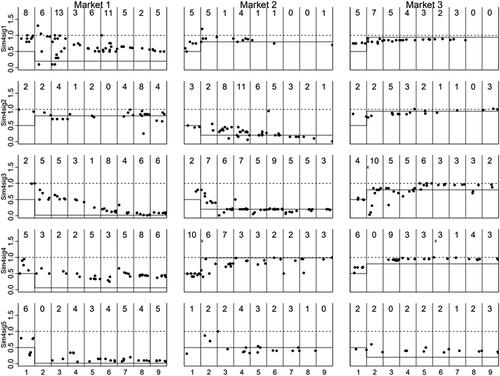
Inspection of the time paths of contract prices and fundamental values reveals that both timing and the number of traders observing signals strongly impact the market. Figures 1–6 report on each our six experimental treatments. Each figure is an array of graphs, with rows corresponding to experimental sessions and the columns to the three market sequences within a session. The sessions of the first four rows are sequential signal release, and the sessions of the last four rows are simultaneous signal release. The horizontal axis of each market graph measures time, the vertical lines indicate market period closings. A dot represents a contract by its time stamp and price (the vertical axis value.) The step function tracks the fundamental value. At the top of each period, we give the total number of trades within that period.

Figure 1. One observer (Pvt) sequential signal sessions; contract prices and fundamental value.

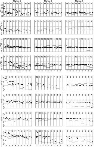
Figure 2. Once observer (Pvt) simultaneous signal sessions; contract prices and fundamental value.

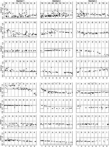
Figure 3. Eight observers (Pub) sequential signal sessions; contract prices and fundamental value.

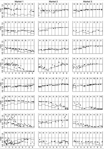
Figure 4. Eight observers (Pub) simultaneous signal observers sessions; contract prices and fundamental value.

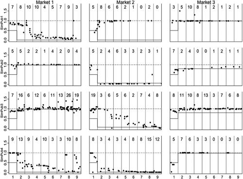
Figure 5. Four observers (4Sig) sequential signal sessions; contract prices and fundamental value.

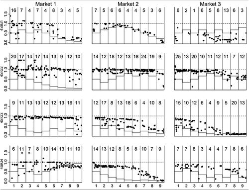
Figure 6. Four observers (4Sig) simultaneous signal sessions; contract prices and fundamental value.

Figures 1 and 2 reveal the absence of any relationship between price and value in the SeqPvt sessions and a weak relationship in the SimPvt ones. There are common features of the price patterns in these experimental sessions. In Market 1, SeqPvt sessions start with variable prices, sometimes well above fundamental value. As the sessions progress, prices become less volatile and unresponsive to changes in value. Eventually, prices lock-in at some level, with the lock-in price often spanning across markets. This is the phenomenon we call a price cascade. When information is simultaneously released, exhibited in Figure 2, this pattern is not as strong. While prices do not equal or even closely approach the fundamental value, in some sessions they do slowly adjust over market periods toward the fundamental value.

We examine corresponding plots for the public treatment (Figures 3 and 4). Again, in both the sequential and simultaneous treatments, we often observe noisy overpricing early on, particularly in Market 1. In Markets 2 and 3, as subjects gain experience, we find successively smaller and shorter duration bubbles, defined as price exceeding either fundamental value or the maximum possible realized value of one, similar to (Smith, Suchanek, and Williams, 1988; Haruvy, Lahav, and Noussair, 2007). With sequential timing, prices noisily track changes in the fundamental value, but generally only approach it in latter periods. This is consistent with other studies in which subjects do not perfectly update according to Bayes rule (Grether, 1980; Charness and Levin, 2005). In contrast, due to the large information release at the end of period 1, prices in the simultaneous sessions usually converge to fundamental value by the end of period 4 or 5, except in a few cases (Notably Market 2 in the SimPub1 session).

Lastly, Figures 5 and 6 present corresponding plots for the Seq4Sig and Sim4Sig treatments. Both treatments exhibit an imperfect relationship between price and value, with Sim4Sig having lower price volatility. To summarize, the price-value plots suggest in all treatments price do not perfectly track the fundamental value. The precision of this tracking increases with the number of observers, and when information is released simultaneously. In the next section, we test whether these visual conjectures can be supported by more formal statistical tests.

Correlation analysis of information aggregation

We quantify the informational aggregation of the different treatments by examining the correlation between price and value. Full aggregation, such that one can perfectly invert the price-value relationship, implies perfect correlation. Table 3 presents the Pearson r correlations for different treatments. We compute these values using each trade as the unit of observation, except for the last row, where we use the mean price in period 9 as the unit of analysis (providing a comparable measure in which each market realization is equally weighted). We compute these correlations for all trades in periods 2 to 9 in the first panel, and period 9 trades in the second panel. The rationale for the analysis in the second panel is that all traders in the two types of timings treatments (sequential and simultaneous) have the same amount information relative to the prior, only in period 9.

Table 3. Correlations between price and fundamental values.

			Pvt		4SIG		PUB
			Seq.	Sim.	Seq.	Sim.	Seq.	Sim.
Periods 2–9	Overall	Pearson r	0.03	0.35	0.36	0.66	0.59	0.77
		Nobs.	1242	1326	919	437	938	521
	Market 1	Pearson r	0.02	0.63	0.10	0.62	0.32	0.77
		Nobs.	491	487	333	175	397	245
	Market 2	Pearson r	−0.10	0.07	0.62	0.75	0.71	−0.10
		Nobs.	400	451	320	144	286	147
	Market 3	Pearson r	0.04	0.25	0.52	0.36	0.9	0.23
		Nobs.	351	388	266	118	255	129
Period 9	Overall	Pearson r	−0.05	0.47	0.47	0.91	0.87	0.81
		Nobs.	145	140	102	45	135	65
	Market 1	Pearson r	−0.61	0.00	0.34	0.81	0.73	0.61
		Nobs.	48	54	36	26	46	34
	Market 2	Pearson r	0.41	0.51	0.64	0.99	0.96	0.53
		Nobs.	39	41	32	8	51	21
	Market 3	Pearson r	0.06	0.77	0.68	0.99	0.94	−0.02
		Nobs.	48	44	34	11	38	10
Mean Period	9 Prices	Pearson r	0.14	0.56	0.48	0.92	0.86	0.93
		Nobs.	23	23	12	13	23	10

Underlined indicates a failure to reject the correlation is zero against the alternative it is positive at the 5% level.

In the SeqPvt treatment, the correlation between price and value is insignificant in all three samples: contract prices from periods 2-9, period 9 contract prices, or average period 9 contract prices. Zero correlation is no information aggregation; the posterior distribution over possible information releases conditional upon any price realization is simply the prior. In other treatments, we find partial to near full information aggregation. All have a significantly positive correlation an overall basis. For both Pvt and 4Sig sessions, simultaneous timing tends to have a higher correlation then sequential timing. For observations computed only using period 9 trades, there is also a pattern of increasing correlations with the number of observers, holding timing fixed.

Regression analysis of the fully revealing rational expectations hypotheses

In a fully revealing competitive equilibrium, price should equal value, which in turn is determined by the union of all information in the market. We assess the extent to which our various treatments adhere to this prediction. First, we present a regression analysis using the mean price in period 9 as the dependent variable, and period 9 value as the independent variable,⁷ (1) $$P_{sm}=\alpha +\beta V_{sm}+{ϵ}_{sm}$$(1) for session s and market m. Under a fully revealing Rational Expectations Equilibrium, we should expect a zero intercept and a $\beta$ coefficient of one. For each of our treatments, we present the results of the OLS estimation of Equation 1(1) $$P_{sm}=\alpha +\beta V_{sm}+{ϵ}_{sm}$$(1) and an F -test that both $\alpha =0$ and $\beta =1$ in Table 4.

Table 4. Regression results of the ninth period trading price mean on fundamental value (robust standard errors) for each treatment.

		SeqPvt	SimPvt	Seq4Sig	Sim4Sig	SeqPub	SimPub
Intercept	Coefficient	0.53	0.36	0.24	0.13	0.12	0.18
	Std. Error	0.07	0.05	0.10	0.07	0.07	0.08
	(p-value)	(0.00)	(0.00)	(0.03)	(0.09)	(0.10)	(0.05)
Value	Coefficient	0.07	0.22	0.36	0.88	0.83	0.89
	Std. Error	0.12	0.07	0.21	0.12	0.11	0.12
R2	(p-value)	(0.53)	(0.01)	(0.11)	(0.00)	(0.00)	(0.00)
		0.02	0.32	0.23	0.84	0.73	0.87
$H_0:\alpha =0 \& \beta =1$	F -stat	34.74	60.78	4.86	2.02	1.49	3.10
	(p-value)	(0.00)	(0.00)	(0.03)	(0.18)	(0.25)	(0.10)
	D.o.f.	21	21	10	11	21	8

Result 1. The Rational Expectations Equilibrium, in prices, is strongly rejected for the SeqPvt, and SimPvt and Seq4Sig treatments, there is weak support for the Sim4Sig, SeqPub and SimPub treatments only in terms of the final market period prices. Hypothesis 1 is not supported.

We start with the results for the SeqPvt treatment. We find $\beta$ is statistically indistinguishable from zero and the estimated value of the constant is 0.53, indistinguishable from the unconditional non-informative value of 0.50. Next, we generally find declining intercepts and increasing $\beta$’s as we increase the number of signal observers while holding the timing fixed (i.e., compare SeqPvt, Seq4Sig, and SeqPub, or SimPvt, Sim4Sig, and SimPub). When comparing the effect of timing, holding the number observers fixed, we find that simultaneous release yields lower intercepts and higher $\beta$’s for the Pvt and 4Sig treatment. For the Pub treatment these coefficients are similar to each other and the rational expectation equilibrium values. When testing for the fully rational expectations equilibrium, we reject it for the SeqPvt, SimPvt, and Seq4Sig treatments only.

Result 2. We strongly reject the comparative price efficiency in favor of unique price formation processes for alternative treatments. Hypothesis 2 is not supported.

In Table 5, we report the results of Chow tests, evaluating whether treatment pairs are homogeneous, i.e., they have common values for the intercept and slope terms. With respect to the number of observers, the Pvt treatment is different than the 4Sig and Pub treatments regardless of the timing. However, we can’t reject homogeneity between the 4Sig and Pub treatments. With respect to timing, Simultaneous and Sequential release are not homogeneous for the Pvt and 4Sig treatments, but homogeneity is not rejected for the Pub treatment.

Table 5. Chow tests of homogeneity in treatment pairs: The number of observers and timing treatment effects.

Observer effects			Timing effects
Comparison	F -stat	p-value	Comparison	F -stat	p-value
SeqPvt vs Seq4Sig	3.61	0.03	SeqPvt vs Sim Pvt	3.79	0.03
SeqPvt vs SeqPub	11.21	0.00	Seq4Sig vs Sim4Sig	3.72	0.04
Seq4Sig vs SeqPub	3.06	0.06	SeqPub vs SimPub	2.07	0.14
SimPvt vs Sim4Sig	23.06	0.00
SimPvt vs SimPub	33.82	0.00
Sim4Sig vs SimPub	0.78	0.47

Analysis of price cascades

In a market with a collection of informative signals, reducing the number of observers for each signal from all traders, to half of the traders, to a single trader reduced the amount of information aggregation. Also, changing the timing of signal release from simultaneous to sequential reduced the amount of information aggregation. In the extreme case of sequential signals, and where each signal observed by a single trader, there was a complete failure of information aggregation. The manner of this failure is a newly documented phenomenon in which a constant price emerged in the market.

We turn our attention to the analysis of this unexpected price cascade phenomenon. We first econometrically establish its presence in the SeqPvt data. Then, we show it was not a product of herding; traders adjusted their portfolios according to privately observed signals. Finally, we suggest that the presence of a large amount noise trades allowed the formation of the price cascades and enabled informed traders to adjust their portfolios without leaking information.

We start by modeling period price levels in the SeqPvt treatment. Consider a specification of the price level that linearly depends upon the previous price, the current change in value, the lagged change in value (allowing for delayed price reaction), and session specific intercepts, ${\alpha }_s$ (which will allow us to test for informational price cascades). (2) $$P_{\mathit{smt}}={\alpha }_s+{\beta }_0\Delta V_{\mathit{smt}}+{\beta }_1\Delta V_{sm,t-1}+{\beta }_2{P}_{sm,t-1}+{ϵ}_{\mathit{smt}}$$(2)

Table 6 presents the results of estimating Equation 2(2) $$P_{\mathit{smt}}={\alpha }_s+{\beta }_0\Delta V_{\mathit{smt}}+{\beta }_1\Delta V_{sm,t-1}+{\beta }_2{P}_{sm,t-1}+{ϵ}_{\mathit{smt}}$$(2) for the SeqPvt treatment. To further validate our results, we estimate this model using the mean, median and closing price as different dependent variables. These models are estimated by feasible generalized least squares with session specific variances because we generally reject the hypothesis of equal variances in each session.⁸ We also test, but do not report, for autocorrelations using the Breusch-Pagan test and do not find evidence for autocorrelation in the error terms for all our presented specifications.

Table 6. Pvt treatment price level regressions (Equation 2(2) $$P_{\mathit{smt}}={\alpha }_s+{\beta }_0\Delta V_{\mathit{smt}}+{\beta }_1\Delta V_{sm,t-1}+{\beta }_2{P}_{sm,t-1}+{ϵ}_{\mathit{smt}}$$(2) ).

Independent variable	Mean price	Media price	Closing price	Stationary price
$\Delta V_{\mathit{smt}}$	−0.066	−0.054	−0.040
	0.075	0.061	0.054
$\Delta V_{sm,t-1}$	0.046	0.059	0.061
	0.072	0.058	0.051
$P_{sm,t-1}$	0.328	0.566	0.564
	0.084 ***	0.068 ***	0.065 ***
${\alpha }_1$	0.259	0.175	0.177	0.40
	0.041 ***	0.035 ***	0.033 ***
${\alpha }_2$	0.330	0.215	0.216	0.49
	0.056 ***	0.045 ***	0.042 ***
${\alpha }_3$	0.358	0.234	0.235	0.54
	0.051 ***	0.043 ***	0.040 ***
${\alpha }_4$	0.397	0.247	0.250	0.57
	0.058 ***	0.046 ***	0.044 ***
${\alpha }_5$	0.396	0.255	0.244	0.58
	0.064 ***	0.052 ***	0.049 ***
${\alpha }_6$	0.441	0.297	0.297	0.68
	0.066 ***	0.055 ***	0.051 ***
${\alpha }_7$	0.609	0.385	0.380	0.89
	0.085 ***	0.069 ***	0.065 ***
${\alpha }_8$	0.446	0.272	0.282	0.60
	0.073 ***	0.062 ***	0.059 ***
Observations	159	159	159
R2	0.61	0.73	0.77
Wald stat. all ${\alpha }_i$ equal	32.660	19.720	22.810
Probility$>{\mathrm{\chi }}^2$	<.0001	0.006	0.002

Turning our attention to the coefficient estimates, we first note that the coefficients of change in value in the current period, $\Delta V_{\mathit{smt}},$ and the lagged change in value, $\Delta V_{\mathit{smt}},$ are statistically insignificant: more evidence of no information aggregation. The estimates for the coefficient on lagged price range from 0.32 to 0.57. Each of these estimated coefficients is significantly different from 1 and standard tests reject the presence of a unit root.⁹

The estimates of the session specific intercepts provide statistical evidence of price cascades. All intercept estimates are significantly different from zero and from each other. This result, along with the coefficient of lagged price being less than one, indicates that prices are session specific mean reversion processes. The corresponding stationary points are the homegrown price norms at which informational price cascades form. Let’s consider the stationary price for a SeqPvt session, denoted $P_{\mathrm{s}}.$ Once an informational price cascade forms, i.e. a stationary point reached, $$P_{\mathit{smt}}={\alpha }_s+{\beta }_2{P}_{\mathit{smt}-1}+{ϵ}_{\mathit{smt}}.$$

If one takes expectations on both sides, then one has the following $$E\left(P_{\mathit{smt}}\right)=\frac{{\alpha }_s}{1-{\beta }_2}.$$

Thus, a non-zero positive intercept implies the presence of a long run steady state price as long as ${\beta }_2$ is less than one. We report the calculated stationary price, using the median price measure¹⁰, for each session in the last column of Table 6. We summarize the regression analysis with the statement of our next result.¹¹

Result 3. The non-aggregation of information in the Pvt treatments manifests itself as informational price cascades. Hypothesis 3 is supported.

Portfolio adjustments

We now consider the question, given the presence of informational price cascades, did traders simply disregard their private information and select asset holdings independent of their private information? In other words, did they herd?

If subjects exploited informational advantages, we should expect to see the final number of asset units held to differ conditional on whether a subject observed a Red or Black draw. However, if subjects were herding, we should see no such differences. In Table 7, we report the average and standard deviation of final market asset holdings conditional upon market number and signal type observed. Using the endowment of five units of the assets as a benchmark, on average those who received a Black signal reduced their holdings by approximately one unit and those who received a Red signal added about one unit. This would suggest subjects were not herding, except the standard deviations are quite large and we can’t reject the hypothesis that average final asset holdings were the same for both Black and Red signal receivers.

Table 7. Average final asset units holdings conditional upon signal.

Signal	Market 1	Market 2	Market 3	Total
Black	4.64	3.72	4	4.13
Stand. dev.	3.58	3.52	3.84	3.65
Red	5.39	6.06	6.37	5.92
Stand. dev.	3.88	4.27	4.46	4.17
Total	5.00	5.00	5.00	5.00
Stand. dev.	3.55	3.97	4.52	4.01

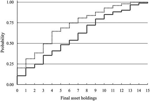
It turns out the high standard deviations in asset holdings arose from an important heterogeneity in how subjects chose portfolios. In Figure 7, we plot the empirical CDF’s of final asset holdings, conditional on receiving a Red or Black signal. There are several features worth noting. First, the supports of both distributions are quite large: zero to thirteen, for those who observed a Black signal; and zero to fifteen, for those who observed a Red signal. Second, many people chose corner solutions: 20% of the Black signal receivers and 10% of the Red signal receivers held zero units of the asset. Finally, casual inspection suggests the empirical CDF of Red first order stochastically dominates that of Black. Formally, a nonparametric hypothesis test suggested by Barrett and Donald (2003) rejects the absence of first order stochastic dominance for any plausible level of significance.¹² Evidently some traders adjusted their portfolios based upon their signals, while at the same time there is tremendous variation in portfolio adjustments.

Figure 7. Empirical CDF of final asset holdings for Red and Black signal receivers, dashed line for Black.

Timing and informational content of market actions

Last, we address the question, how were some subjects able to use their private information to make profitable portfolio adjustments without transmitting this information to the market? It turns out they were able to do so because many of the other subjects, who were not informed, are also engaged in trades. This created a large amount of noise trades, diluting the informational content of the informed trader’s market actions.

We examine the price and the identities of the transacting parties to determine whether a given trade revealed information about the last observed draw. Any trade between two non- informed traders is called a noise trade. A trade involving the informed trader, the one who observed the last signal, will be classified as either informative or non-informative. We argue an informative trade occurs when the informed trader takes an action that allows others (conditional upon knowing the trader’s action and identity) to infer the period’s signal.

We start by assuming, rather dubiously, that any impact a signal had on price was realized by the end of the trading period and was reflected in the closing price. So, when assessing the informational content of a trade, we consider whether the price was an increase or decrease from closing price of the previous period. Under what types of actions did an informed trader reveal the value of her signal? Consider the following scenario – suppose the informed trader bought a unit at a price higher than the previous closing price. Was this purchase rational given the observed signal? Clearly, the informed trader would not have purchased if the signal was Black, because that signal would cause her expectation of the dividend to fall below the previous closing price. However, if the signal was Red, then her expected value of the dividend would have increased, and purchasing the asset at a higher price was rationalizable. Thus, buying at a higher price separated the two possible signals and provided information to the market. Now, let’s suppose the informed trader was the seller, rather than the buyer. Selling at a higher price was rational irrespective of whether the signal was Red or Black, hence this trade provided no new information to the market. We call such a trade as non-informative. Note that there was a possibility that an informed trader who saw a Black signal still bought at a higher price – thus violating the rationality described before. We classify this type of contrarian trade also as non-informative. From similar arguments, a price decrease from the previous closing price was informative only if the informed trader was a seller, which would only have been rational if the signal was Black. Table 8 shows how we sort different trades into different categories.

Table 8. Sorting rules of trades into noise, informative, and non-informative classifications.

Price change	Signal	Informed trader role	Classification
–	–	None	Noise
Positive	Red	Buyer	Informative
Positive	Red	Seller	Non-informative
Positive	Black	Either	Non-informative
Negative	Black	Seller	Informative
Negative	Black	Buyer	Non-informative
Negative	Red	Either	Non-informative
None	Either	Either	Non-informative

With these classifications of signals, we calculate the proportion of informative signals. Figure 8 plots the results of trades classified as above with the order of the trade within a given period – the idea being to examine how long it takes for the informed trader’s information to be incorporated into the price.

Figure 8. Count of informative, noninformative, and noise contracts according to trade number in period.

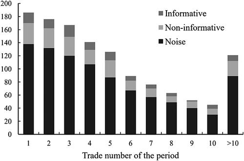
The figure vividly exhibits two features. First, a large proportion of trades are noise trades, i.e., trades where both participants do not have any information in the given period. For example, for the first trade in any given period, about seventy-five percent are noise trades. This pattern continues for most trades. A second even more striking fact is that less than 50% of the informed subjects’ trades are actually informative.

Consider the following thought experiment. If an outsider wanted to infer the likelihood that the insider obtained a positive signal in a given period, then observing the opening trade of the next period being transacted at a higher price relative to the previous period, the chance of the trade reflecting positive information is only around 10%-15%. This provides a strong reason for the lack of aggregation. The proportion of informative trades is too low relative to the total number of trades. Overall, the large presence of noise traders transacting at a homegrown price norm compounded the lack of information aggregation, as informed traders can make portfolio adjustments without affecting the price.

Conclusion

We conclude by discussing how our study and findings relate to the existing experimental literature, and suggesting future directions of inquiry. Our initial premise asked if the long-lived asset, and accompanying long sequence of informative private information, of Bikhchandani, Hirshleifer, and Welch traded in a market with decentralized private information leads to full information aggregation or informational cascades. They were strong precedents that the information should aggregate in our experiment. In particular, in the social learning literature, it’s been robustly shown theoretically (Avery and Zemsky, 1998) and experimentally (Drehmann, Oechssler, and Roider, 2005; Cipriani and Guarino, 2005) that allowing for rational market makers, who endogenously set prices, information fully aggregates. Further, in experimental tests of fully revealing rational expectation equilibrium, information robustly aggregates and efficient pricing occurs with homogeneous preferences, one-period lived assets, and aggregate certainty (Plott and Sunder, 1988). In studies that follow the same Plott and Sunder design except environments with aggregate uncertainty, such as Forsythe and Lundholm (1990) and Bruguier, Quartz, and Bossaerts (2010), information aggregation and the rational equilibrium solutions do not perform as well, although still better than competing theories.

There are a couple of studies that test the fully revealing rational expectation equilibrium with longer lived assets and dynamically arriving private information. Copeland and Friedman (1987, 1991) examine information aggregation in a four-period asset market in which a different subset of subjects learn the true dividend state each period. While they find imperfect adherence to the rational expectations equilibrium, the rational expectation equilibrium still outperforms alternative models. In Barner, Feri, and Plott (2005), there is a three-period lived asset with four possible dividend levels. Subjects are partitioned and each period an element of the subject partition is informed of one of the non-realized states; hence aggregate certainty is achieved in the last period of the market. Each subject partition always has multiple traders so there is no treatment like our Pvt one. With this structure, they find much more support for the rational expectation equilibrium and information aggregation hypothesis than we do.¹³ The above suggest that aggregate uncertainty leads to reduced informational efficiency, but typically not enough to reject the fully revealing rational expectations equilibrium in favor of alternative equilibrium models.

A second potential reason for the lack of aggregation in our experiment, in contrast to social learning experiments, is the endogenous timing of trades. The only effort we are aware of that incorporate flexible prices with endogenous timing is the experimental study by Park and Sgroi (2012) in which subjects are provided signals of heterogeneous strength prior to trading. Their focus however is on the effects of differentially precise signals and its impact on the actions of insiders. However, it should be noted that a subject can make at most two transactions and therefore is still different from the experiment in this paper.

This complete freedom for timing of trades creates a large amount of trading, both for insiders as well as for noise trades. Theoretically, we know that this timing option should create partial aggregation (Kyle (1989)) but not cascades. Empirically, Bloomfield, O’Hara, and Saar (2009) observe that when the number of non-informed traders increases price efficiency is reduced when the realized value is far from the prior expected value, but price efficiency increases when that difference is small. Further, informed traders tend to wait until the latter part of the period to trade. While we do not observe a temporal pattern of insider trading within a round, and noise trading is not a treatment variable in our experimental set up, we document similar results except that in our set up this actually leads to cascades. Thus, the endogenous timing option for insider trading appears also be an important ingredient for informational cascades.

We have demonstrated that market and social learning are not equivalent, and one should be careful in extrapolating the results of social learning models to asset markets. However, our results also suggest new questions. Is there either an equilibrium or behavioral foundation for the price cascade phenomenon? In terms of further experimental inquiry there are several avenues of interesting inquiry including sequences of shorter-lived assets, settings with aggregate certainty, and would public signals alongside private ones trigger price responses that cause information to flow back into the market. Finally, can price cascades be observed in equity markets? Clearly such mispricing would be important but difficult to identify.

Additional information

Funding

Jason Shachat acknowledges funding from the ESRC under project ES/P011829/1.

Notes

1 The prediction of full information aggregation occurs only under some conditions.

2 This treatment was introduced by Palfrey and Wang (2012) to study speculation and rational overpricing arising from heterogeneous biases in updating posterior beliefs regarding an assets fundamental value.

3 A sample set of instructions are provided in the appendix, sets of instructions for all treatments are available from the authors upon request.

4 This laboratory is especially designed to conduct research experiments with individual computers housed in private carrels that prevent subjects from viewing each other’s computer screens and also discourage communication between subjects.

5 The experiment includes three markets to facilitate traders gaining experience. In the popular design of experiments of long-lived assets introduced by Smith, Suchanek, and Williams (1988), markets with twice experienced subjects generally achieve full price efficiency. Shachat and Wang (2014) show there is minimal efficiency loss when this experience is garnered in a single experimental session our across multiple sessions.

6 Attentive readers may notice that while we maintain the same null hypothesis and definition of rational expectations as Plott and Sunder (1988), we have replaced their alternative hypothesis of the prior information equilibrium (Lintner, 1969) with one of informational cascades. The prior information equilibrium incorporates a price the reflects only the public prior information, while our informational cascade hypothesis encompasses a larger set of price sequences which we assert is more appropriate for the more dynamic environment of our study.

7 To compare the aggregation across the two treatments, it would be more appropriate to do so when the total information in the market is similar, i.e., during the last period of trading, when the market as a whole received 8 signals about the final value.

8 The null hypothesis of homoscedasticity is rejected in all specifications except for closing price.

9 Due to the small number of observations in each session, these unit root tests are conducted by taking all the end of period observations of each treatment and stacking them together.

10 We use the coefficients from the regression on the median price because it always results in a value that lies between the same calculations based upon the mean and closing price regressions. Note that the difference between these calculated values is never more than five cents.

11 We conduct a variety of robustness checks of these results, including controlling for the impact of trader experience, and the presence of bubbles. The details of these checks are available in the SSRN version of the working paper (http://ssrn.com/abstract=1813383). In brief, the main finding is that accounting either for bubbles or experience, does not alter the result of zero aggregation of information in the Pvt treatment.

12 The test-statistic is $z*{(\frac{mn}{m+n})}^{0.5}$ where m and n are the number of observed Black and Red draws respective, and z is the absolute of maximum difference between the two empirical CDF’s. The p-value of this statistic is $\text{exp}\hspace{0.17em}(-2*z^2).$

13 However, there are significant pricing inefficiencies as they do find some mirages (price moving the opposite direction of the signal) and bubbles (price moves in the direction suggested by the signal but to the price above the fundamental value).

Appendix A

A Sample Instructions: 4Sig Treatment

Experimental instructions (please read along quietly while the experimenter reads aloud.)

You are now participating in an experiment which studies decision making in Asset markets. Contingent on your decisions in this experiment, you can earn money in excess of your participation fee of S$10. Hence, it is important that you read these instructions very carefully.

Also, we request you do not use hand phones, laptop computers, or use the lab’s desktop computer except for the experimental software application. You may read quietly if there is a lull. Please refrain from talking for the duration of the experiment, or looking at other’ computer monitors. If at some point you have a question, please raise your hand and we will address it as soon as possible. If you do not observe these rules, we will have to exclude you from this experiment and all associated payments, and ask you to leave.

The experiment consists of four consecutive markets. The first market will last for three periods and is solely for practice. You will not receive any earnings. The last three markets will last nine periods each; and you will receive any associated earnings in Singapore dollars. All payments to you will be privately made at the conclusion of the experiment.

We next will answer the following two questions?

1. What is the asset that we will trade?

2. How does the trading system work?

A.1 what is the asset we will trade?

In each market, there is a single type of asset you can buy or sell. This asset only pays a dividend after the last round, and this dividend will either be $0 or $1. The asset holds no value other than this dividend. Prior to each of the four markets, we will determine the value of this by tossing a fair coin. If the coin lands Flower face up then the dividend will be $0, and if the coin lands Crest face-up, the dividend will be $1. Thus, there is a fifty percent chance the dividend is $0 and a fifty percent chance the dividend is $1. Note, we will not reveal the value of the dividend until AFTER the last round of trading.

However, we will provide information relevant to the true value of the dividend after the first round of trading in each market. For each market, after tossing the coin, and prior to the beginning of trading, we will randomly select a chip from an urn that contains Red and Black chips and then RETURN that chip to the urn. Knowledge of the chip color is important because the number of Red and the number of Black chips placed in the urn is determined by the true value of the dividend. If the dividend is 0 we will place four (4) Red and eight (8) Black chips in the bowl. On the other hand, if the dividend is 1 we will place eight (8) Red chips and four (4) Black chips in the bowl.

We repeat this process of drawing chips from the urn seven more times (thus, a total of eight independent draws from the urn). For each draw, we will reveal the color only to four, or one-half, of the participants. We do this by randomly dividing you and the other participants into two equally sized groups. Membership in the groups is private and you will not know who else is in your group. One group of four will be shown the color of the chip selected in the first draw, and the other group of four is shown the color of the chip selected in the second draw. We will again randomly divide the eight participants into two groups of four, and repeat this process. We do this two more times, thus the total number of times chips are drawn is eight, and each participant gets to observe four of these eight outcomes (RED or BLACK). Note that each of the outcomes observed by a given participant is also observed by exactly three other participants.

We adopt the following protocol to keep the recipients of the information anonymous. At the end of the first round of trading in each market, you will see the four outcomes written on a piece of paper given to you in an envelope. When you receive your envelope each period you must view the contents carefully, and you must not communicate or show others the content. After inspecting the contents keep this slip of paper back in the envelope. Someone will come and collect the envelope.

Lastly, we address the issue of what assets and currency one has available to make trades in the market. Prior to the first round of trading in each market, every participant in the market will be given five (5) units of the asset and $5. There will be no other disbursement of currency or units of the asset in that market. You currency balance and inventory of assets will carry over in each round of trading. You may sell a unit of the asset as long as your inventory has at least one unit, and you may buy a unit of the asset as long as you have sufficient currency on hand. After the last round of trading, the dividend will be paid on each asset. You earnings will be the sum of your dividends and your final currency balance, and the participation fee of $10.

A.2 how does the trading system work?

The trading system is a so called continuous double auction, i.e., at any point during a trading period, you can act as buyer or seller.

The market view has four areas.

1. The right-hand side of the screen provides “Information on your holdings.” Here, you will find your Starting Balance (currency carried over from the previous period,) Endowment (currency you receive from the experimenter – for this experiment $5 and only in period 1), Dividend payouts from previous period (will always be zero in this experiment except for the last period), Current Balance, Current Bid balance (currency you have committed to bids in the current trading period), and Available Balance (amount of currency on hand with which you can generate new bids or purchases at current asks). This is also where you can view your inventory of the Asset.

2. The bottom row displays the sequence of prices for unit of the asset for the current trading period.

3. The lower left corner is the area in which you take market actions. Here you can click on the ‘Buyer Actions’ tab to submit a bid price to the market at which you are willing to purchase a unit, or you can click on the ‘Buy’ button to purchase a unit at the current lowest ask price in the market. Here, you can also click on the ‘Seller Actions’ tab to submit an ask price to the market at which you are willing to sell a unit, or you can click on the ‘Sell’ button to sell a unit at the current highest bid in the market.

4. The upper left corner contains information on current market conditions (all participants see this information except which bid/ask belong to specific other participants.) ‘Queues’ are the lists of the current bids and asks that have been submitted to the market but have not yet been selected. Your outstanding bids and asks will be marked with an asterisk to the right of them. The ‘Bid-Ask’ Spread gives the current (lowest available) ask price to sell and the current (highest available) bid to purchase.

A.3 how to make trades?

As suggested, there are four types of actions you can take in a trading period; submit a bid price to purchase, and ask price to sell, purchase by accepting the lowest outstanding ask, and sell by accepting the highest outstanding bid. You can also do these in any sequence you want. For example, you can simultaneously have an outstanding bid, an outstanding ask, and then purchase at the lowest ask in the market (as long as it isn’t your outstanding ask.) You may also have multiple outstanding bids and/or asks at a given time.

There are some basic rules governing what bids and asks you may submit. 1) When you submit a new bid, it must be at least as large as the current bid and you must have at least the bid amount of currency available. 2) When you submit a new ask, it must be at least as small as the current ask and you must have at least one unit of the Asset in inventory (Note, when you successfully submit an ask, your inventory of available assets is reduced by one.)

3) If you attempt to buy a unit at the current ask, then you must have enough available currency and you can’t attempt to purchase from yourself. 4) If you attempt to sell at the current bid, you must have a unit available and you can’t sell to yourself. 5) All bids and asks will be stored in the queues, you may withdraw any bid or ask you submit as long as it is neither the current bid or ask. To withdrawal a bid or ask, highlight in the list found in the lower left corner and click the retract button.

When a contract occurs, the associated bid or ask is removed from the bid-ask queues. If you are involved in the contract, your currency holdings and asset inventory will be automatically adjusted. Finally, when the trading period ends, all bids and asks are removed from the queue (and the associated asset units and currency are credited back to the participants) To summarize, you may purchase a unit of the asset in two ways; you may submit a bid price to buy that becomes the current bid and another participant ‘sells’ to you, or you may choose to ‘buy’ at the current lowest ask. Likewise, you may sell an asset in two ways; you may submit an ask price to sell that becomes the current ask and another participant ‘buys’ from you, or you may choose to ‘sell’ at the current highest bid.

Remember, each market has nine trading periods. Each of the trading periods will last 1.5 minutes. The practice market is an exception; it will have only three 2.5 minute trading periods. We will privately flip a coin to determine the final dividend value of the asset prior to the market. After each trading period, we will draw a chip from an urn whose composition is determined by the true dividend value. After the last trading period of the market, the value of the dividend will be revealed and your market earnings calculated.

At this time please locate the small window on your monitor titled login. Locate the box host, it should have a number that is the same as the one written on the whiteboard. If not click on the down arrow tab and that number should be on the list. Select it. Next, enter your student matric number into the username field (all CAPITAL LETTERS). Then click connect. You will receive a message asking you to wait for the experiment to start. If you can’t reach this step raise your hand and someone will come and assist you.

References

- Alevy, Jonathan E., Michael S. Haigh, and John A. List. 2007. “Information Cascades: Evidence from a Field Experiment with Financial Market Professionals.” The Journal of Finance 62 (1):151–80. doi:10.1111/j.1540-6261.2007.01204.x
- Anderson, Lisa, and Charles A. Holt. 1997. “Information Cascades in the Laboratory.” American Economic Review 87 (5):847– 62.
- Avery, Christopher, and Peter Zemsky. 1998. “Multidimensional Uncertainty and Herd Behavior in Financial Markets.” American Economic Review 88 (4):724–48.
- Barner, Martin, Francesco Feri, and Charles R. Plott. 2005. “On the Microstructure of Price Determination and Information Aggregation with Sequential and Asymmetric Information Arrival in an Experimental Asset Market.” Annals of Finance 1 (1):73–107. doi:10.1007/s10436-004-0005-4
- Barrett, Garry F., and Stephen G. Donald. 2003. “Consistent Tests for Stochastic Dominance.” Econometrica 71 (1):71–104. doi:10.1111/1468-0262.00390
- Bikhchandani, Sushil, David Hirshleifer, and Ivo Welch. 1992. “A Theory of Fads, Fashion, Custom, and Cultural Change as Informational Cascades.” Journal of Political Economy 100 (5):992–1026. doi:10.1086/261849
- Bloomfield, Robert, Maureen O’Hara, and Gideon Saar. 2009. “How Noise Trading Affects Markets: An Experimental Analysis.” Review of Financial Studies 22 (6):2275–302. doi:10.1093/rfs/hhn102
- Bruguier, Antoine J., Steven R. Quartz, and Peter Bossaerts. 2010. “Exploring the Nature of “Trader Intuition.” The Journal of Finance 65 (5):1703–23. doi:10.1111/j.1540-6261.2010.01591.x
- Camerer, Colin F. 1987. “Do Biases in Probability Judgment Matter in Markets? Experimental Evidence.” American Economic Review 77 (5):981–97.
- Celen, Bogachan, and Shachar Kariv. 2004. “Distinguishing Informational Cascades from Herd Behavior in the Laboratory.” American Economic Review 94 (3):484– 98. doi:10.1257/0002828041464461
- Charness, Gary, and Dan Levin. 2005. “When Optimal Choices Feel Wrong: A Laboratory Study of Bayesian Updating, Complexity, and Affect.” American Economic Review 95 (4):1300–9. doi:10.1257/0002828054825583
- Cipriani, Marco, and Antonio Guarino. 2005. “Herd Behavior in a Laboratory Financial Market.” American Economic Review 95 (5):1427–43. doi:10.1257/000282805775014443
- Cipriani, Marco, and Antonio Guarino. 2009. “Herd Behavior in Financial Markets: An Experiment with Financial Market Professionals.” Journal of the European Economic Association 7 (1):206–33. doi:10.1162/JEEA.2009.7.1.206
- Copeland, Thomas E., and Daniel Friedman. 1987. “The Effect of Sequential Information Arrival on Asset Prices: An Experimental Study.” The Journal of Finance 42 (3):763–97. doi:10.1111/j.1540-6261.1987.tb04585.x
- Copeland, Thomas E., and Daniel Friedman. 1991. “Partial Revelation of Information in Experimental Asset Markets.” The Journal of Finance 46 (1):265–95. doi:10.1111/j.1540-6261.1991.tb03752.x
- Corgnet, Brice, Mark DeSantis, and David Porter. 2020. “The Distribution of Information and the Price Efficiency of Markets.” Journal of Economic Dynamics and Control 110:103671. doi:10.1016/j.jedc.2019.02.006
- Corgnet, Brice, Mark DeSantis, and David Porter. 2021. “Information Aggregation and the Cognitive Make-up of Market Participants.” European Economic Review 133:103667. doi:10.1016/j.euroecorev.2021.103667
- Cox, JamesC, and JTodd Swarthout. 2006. “EconPort: Creating and Maintaining a Knowledge Commons.” In Understanding Knowledge as a Commons: From Theory to Practice, edited by Charlotte Hess and Elinor Ostrom, 333–48. Cambridge: MIT Press.
- Diamond, Douglas W., and Robert E. Verrecchia. 1981. “Information Aggregation in a Noisy Rational Expectations Economy.” Journal of Financial Economics 9 (3):221–35. doi:10.1016/0304-405X(81)90026-X
- Drehmann, Mathias, Jörg Oechssler, and Andreas Roider. 2005. “Herding and Contrarian Behavior in Financial Markets: An Internet Experiment.” American Economic Review 95 (5):1403–26. doi:10.1257/000282805775014317
- Forsythe, Robert, and Russell Lundholm. 1990. “Information Aggregation in an Experimental Market.” Econometrica 58 (2):309–47. doi:10.2307/2938206
- Foster, F. Douglas, and S. Viswanathan. 1996. “Strategic Trading When Agents Forecast the Forecasts of Others.” The Journal of Finance 51 (4):1437–78. doi:10.1111/j.1540-6261.1996.tb04075.x
- Ganguly, Ananda R., John Kagel, and Donald V. Moser. 2000. “Do Asset Market Prices Reflect Traders’ Judgment Biases?” Journal of Risk and Uncertainty 20 (3):219–45. doi:10.1023/A:1007848013750
- Goeree, Jacob K., Thomas R. Palfrey, Brian W. Rogers, and Richard D. McKelvey. 2007. “Self-Correcting Informational Cascades.” The Review of Economic Studies 74 (3):733–62. doi:10.1111/j.1467-937X.2007.00438.x
- Grether, David M. 1980. “Bayes Rule as a Descriptive Model: The Representativeness Heuristic.” The Quarterly Journal of Economics 95 (3):537–57. doi:10.2307/1885092
- Grossman, Sanford J. 1976. “On the Efficiency of Competitive Stock Markets Where Traders Have Diverse Information.” The Journal of Finance 31 (2):573–85. doi:10.1111/j.1540-6261.1976.tb01907.x
- Haruvy, Ernan, Yaron Lahav, and Charles Noussair. 2007. “Traders’ Expectations in Asset Markets: Experimental Evidence.” American Economic Review 97 (5):1901–20. doi:10.1257/aer.97.5.1901
- Hayek, F. A. 1945. “The Use of Knowledge in Society.” The American Economic Review 35 (4):519–30.
- Hirshleifer, David. 2001. “Investor Psychology and Asset Pricing.” The Journal of Finance 56 (4):1533–97. doi:10.1111/0022-1082.00379
- Holden, Craig W., and Avanidhar Subrahmanyam. 1992. “Long-Lived Private Information and Imperfect Competition.” The Journal of Finance 47 (1):247–70. doi:10.1111/j.1540-6261.1992.tb03985.x
- Hurwicz, Leonid. 1972. “On Informationally Decentralized Systems.” In Decision and Organization: A Volume in Honor of Jacob Marschak, edited by C. B. McGuire and Roy Radner, 425–59. Amsterdam: North-Holland.
- Kyle, Albert S. 1989. “Informed Speculation with Imperfect Competition.” The Review of Economic Studies 56 (3):317–55. doi:10.2307/2297551
- Lintner, John. 1969. “The Aggregation of Investor’s Diverse Judgments and Preferences in Purely Competitive Security Markets.” The Journal of Financial and Quantitative Analysis 4 (4):347–400. doi:10.2307/2330056
- Lucas, Robert. Jr. 1972. “Expectations and the Neutrality of Money.” Journal of Economic Theory 4 (2):103–24. doi:10.1016/0022-0531(72)90142-1
- Page, Lionel, and Christoph Siemroth. 2020. “How Much Information is Incorporated in Financial Asset Prices? Experimental Evidence.” Review of Financial Studies, forthcoming.
- Palfrey, Thomas R., and Stephanie W. Wang. 2012. “Speculative Overpricing in Asset Markets with Information Flows.” Econometrica 80 (5):1937–76.
- Park, Andreas, and Daniel Sgroi. 2012. “Herding, Contrarianism and Delay in Financial Market Trading.” European Economic Review 56 (6):1020–37. doi:10.1016/j.euroecorev.2012.04.006
- Plott, Charles R., and Shyam Sunder. 1988. “Rational Expectations and the Aggregation of Diverse Information in Laboratory Security Markets.” Econometrica 56 (5):1085–118. doi:10.2307/1911360
- Radner, Roy. 1979. “Rational Expectations Equilibrium: Generic Existence and the Information Revealed by Prices.” Econometrica 47 (3) :655–78. doi:10.2307/1910413
- Sgroi, Daniel. 2003. “The Right Choice at the Right Time: A Herding Experiment in Endogenous Time.” Experimental Economics 6 (2):159–80. doi:10.1023/A:1025357004821
- Shachat, Jason, and Hang Wang. 2014. “Are You Experienced?.” MPRA Paper 57672, University Library of Munich, Germany.
- Smith, Vernon L., Gerry L. Suchanek, and Arlington W. Williams. 1988. “Bubbles, Crashes, and Endogenous Expectations in Experimental Spot Asset Markets.” Econometrica 56 (5):1119–51. doi:10.2307/1911361
- Vives, Xavier. 1995. “The Speed of Information Revelation in a Financial Market Mechanism.” Journal of Economic Theory 67 (1):178–204. doi:10.1006/jeth.1995.1070