
 ?Mathematical formulae have been encoded as MathML and are displayed in this HTML version using MathJax in order to improve their display. Uncheck the box to turn MathJax off. This feature requires Javascript. Click on a formula to zoom.
Abstract
Within the context of a shared on-demand transport system, we study the problem of selecting the stopping points from which passengers should walk to their exact destinations (or from their exact origins). We focus on the single-vehicle case that must follow a predefined order of requests, posing the mathematical program, showing that it can be solved in polynomial time and proposing a heuristic that runs faster. We compare the optimal algorithm, the heuristic, and the routes that visit the exact request points, and we show that avoiding detours can reduce total costs by almost one fifth and vehicle costs by more than one third. The heuristic yields competitive results. Simulations over the real street network from Manhattan show that the time reduction achieved by the heuristic might be crucial to enable the system to operate in real-time.
Introduction
Transport and network researchers have studied on-demand systems for a long time. The DAR (dial-a-ride) problem was analyzed widely during the seventies and eighties (for example Jaw et al., Citation1986; Psaraftis, Citation1983; Wilson et al., Citation1976), usually assuming trips requested by phone. In the past few years, the problem has gained new attention due to the massive coordination abilities provided by online (real-time) apps (as shown by Uber or Cabify), which changes the problem as now there are many more requests, and they arrive more often. This increase in the number of users enhances the possibility of using shared systems, in which different users can ride the same vehicle at the same time,Footnote1 making these systems more similar to public transport systems, and the problem also related to VRP (vehicle routing problem). Martinez and Crist (Citation2016), Alonso-Mora et al. (Citation2017), and Fagnant and Kockelman (Citation2018), for instance, study different ways to operate such systems in Lisbon, Manhattan, and Austin, respectively. They all assume a driverless technology, which also favors the massiveness of this type of system by reducing the operating costs. Nevertheless, they act as private taxis when dealing with their routes, as they carry every passenger from their specific origin to their specific destination, rather than requesting them to walk to/from nearby points.Footnote2
Traditional public transport systems (with fixed routes) collect users in stops for two main reasons: 1) to gather enough passengers close to those routes, and 2) to avoid unnecessary detours. The first reason becomes irrelevant when vehicles can coordinate online with users; but the second one is still valid, such that there is a tradeoff between shortening these detours and preventing passengers from walking long distances. Moreover, on-demand systems do not need to rely on predetermined meeting points, but they can be decided online, adjusting to each vehicle’s route.
To illustrate the potential benefits of users’ walks, consider and based on real-world examples. shows snapshots from Google Maps in Santiago, Chile, for a vehicle that’s on its way to pick up (or drop off) a passenger. If walks are not admitted and the service is door-to-door, a detour of three minutes is required to arrive at the passenger’s exact origin. On the other hand, if the system can require users to walk, then this passenger needs to walk a very short distance to meet the vehicle in the same street its currently driving, inducing zero detour. Note that in this case, the savings are mostly justified by the directions of the streets.
Figure 1. Snapshots from Google Maps in Santiago, Chile, showing (a) the detour induced to a vehicle if it needs to pick a passenger in his/her door, (b) the walk required by the same passenger to meet the vehicle.
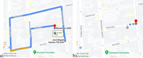
Figure 2. The corner between (a) Huis te Landelaan, a fast street, and (b) Van Vredenburchweg, a slow street, in Rijswijk, The Netherlands.
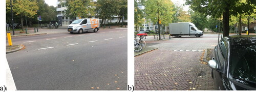
is not related with those directions, but with the velocity of each street. It shows pictures from a real corner in Rijswijk, Netherlands, in which one of the streets involved is fast, and the other one is very narrow and cars share the space with bicycles. If a ridesharing vehicle is driving through the fast street, and needs to pick up (or drop off) a passenger in a point that lays over the slow street, then going to the exact point will induce a severe delay, that would be saved if the passenger can walk to the said corner.
In this paper, we study how to optimize the route of a vehicle that needs to visit some requested points, which might be origins or destinations, but not necessarily at their exact locations, facing a tradeoff between the vehicle’s costs and users’ walking costs. Introducing users’ walks when optimizing a full ridesharing system (i.e., when deciding the assignments between passengers and vehicles at the same time) is a quite complex problem. For instance, in a previous work (Fielbaum et al., Citation2021) we have extended the assignment model by Alonso-Mora et al. (Citation2017) to include the optimization of where to pick-up and drop-off the users: results are promising, but methods have to be specifically designed for the assignment algorithm, which hinders the analysis of the impact of avoiding detours from a more general perspective; this is likely to be the case for any method that optimizes everything together, because of the complexity of the assignment problem by itself, that combines DAR with the VRP, two traditional NP-Hard problems. This is why we focus on a single vehicle, which allows us to provide neat algorithms and results; moreover, the methods proposed here are suitable for the many different ways of modeling and solving ridesharing systems, that include agent-based models (such as Fagnant & Kockelman, Citation2018, or Martinez & Crist, Citation2016) and algorithmic approaches (such as Alonso-Mora et al., Citation2017, or Tsao et al., Citation2019).
State of the art
On-demand mobility systems have been increasingly studied in the last few years, both in shared and non-shared versions. Different types of shared systems (including the ones in which drivers have their own itinerary, and passengers sharing vehicles with cargo) have been surveyed by Mourad et al. (Citation2019), while Silwal et al. (Citation2019) reviews ridesharing systems with an emphasis on their operational architectures. Carsharing systems (in which rides might be non-shared), on the other hand, have been surveyed by Narayanan et al. (Citation2020) and by Wang and Yang (Citation2019).
The single-vehicle problem with flexible pick-up and drop-off locations within an on-demand ridesharing framework, has been studied by Li et al. (Citation2016), in which they also optimize the order in which these points are visited, a problem that is naturally NP-Hard as it extends TSP (traveling salesman problem). However, assuming that the order is endogenous might be troublesome:
Unless we assume that passengers have a common origin or a common destination (which would limit severely the range of application of this problem), the order must include some precedence constraints, namely that pick-ups must occur before drop-offs.
Not all requests emerge at the same time, which might require some orders that are close to some FIFO rules, to keep waiting times bounded for all, and to ensure that the vehicle arrives not before the passenger.
Taking all this into account would again be specific to the ridesharing method and to the assignment algorithm, limiting the generality of the results.
These reasons make the problem in which the order of the visits is fixed but the exact location is optimized a natural one, which has not been studied from a theoretical point of view.
In logistics, a similar problem has also been studied for a single vehicle: a truck delivering some goods, that can use a drone to visit the exact customers’ locations (similar to “walking”), while the truck continues to move toward the following customer, optimizing the places in which the drone is launched (Carlsson & Song, Citation2018). They, too, optimize the order in which the requests are visited, although they discuss the case in which this order exogenous. As in our problem, the extra freedom provided by the drone (like the walking user) allows defining a more direct route for the main vehicle, reducing the detours. However, three structural aspects of the problem are different in comparison with ours, implying significant modeling and mathematical differences:
First, they work over the Euclidean space, because the drone can move unaffected by the road network and the traffic, which allows using several continuous and geometrical tools that are not available in this combinatorial version.
Second, when studying people’s mobility, each user’s time and need to be taken into account, whereas in logistics, one can consider just the total circuit time (as done by Carlsson & Song, Citation2018). This means that what counts is how the truck and the drone effectively coordinate to advance simultaneously, rather than achieving low times for both the car and the walking user, as we do here. Among other implications, this makes the objective function to consider the maximum between the truck’s and drone’s times, instead of the sum of the vehicle’s and user’s times.
Third, because the logistics scheme works with a single drone, the vehicle’s route needs to allow the drone to go back and forth each time, which implies that the location of a customer relates directly with two consecutive truck’s stops: where the drone is launched and the last point it might land. In our problem, each vehicle’s stop is related only with one request, representing either a pick-up or a drop-off, which naturally entails differences in the respective objective functions and the resulting optimal routes.
A few previous papers, besides the ones already described (Carlsson & Song, Citation2018; Fielbaum et al., Citation2021; Li et al., Citation2016), study avoiding-detours on-demand systems from diverse perspectives. Zhao et al. (Citation2018) propose a mathematical model in a non-shared on-demand scheme that optimize where to pick-up and drop-off the passengers. Stiglic et al. (Citation2015) and Li et al. (Citation2018) also solve the complete problem, but they impose a pre-defined set of “meeting points” to which all passengers have to walk, and that are selected from a subset of the nodes. Fielbaum (Citation2020) studies a feeder transit system in which users need to get gathered at some optimized point, but over a simplified city model; a similar approach is followed by Daganzo (Citation1984) under a dial-a-ride scheme, who analyzes under which scenarios it is best to use fixed lines or a flexible dial-a-ride system that might have fixed meeting points. Finally, Pei et al. (Citation2019) and Zheng et al. (Citation2019) also consider meeting points for “flex-route” systems, in which traditional transit routes are allowed to make constrained changes on-demand.
While a new topic for on-demand systems, the tradeoff between walking and vehicles’ routes has been thoroughly studied in public transport. Hurdle (Citation1973), Kocur and Hendrickson (Citation1982), and Chang and Schonfeld (Citation1991) have studied systems formed by parallel transit lines, to optimize their spatial density. More complex systems have been analyzed by Daganzo (Citation2010) and Badia et al. (Citation2014), who optimize spatial density when considering bus transit networks, and by Tirachini et al. (Citation2010), who compare different modes. On a related note, Tirachini (Citation2014) optimizes the distance between bus stops, which affect passengers’ walks and vehicles’ speed, although not their routes. All these papers provide some intuition regarding ridesharing systems, as they propose sound methodologies to optimize operators’ and users’ costs jointly, and they show that walks can be beneficial not only for operators but also for users (at least partially), by reducing waiting and in-vehicle times. However, as public transport provides fixed routes (as opposed to on-demand), there are also structural differences with on-demand ridesharing systems; in particular, one expects that latter can still provide door-to-door service to requests that do not induce relevant detours.
Contribution and organization of this paper
The problem of optimizing the route of a single shared vehicle that must serve a fixed order of requests, in which users might be requested to walk to a different node, has not been studied from a theoretical point of view. In this paper we fill that gap. We show that this problem can be optimized with a polynomial algorithm, whose complexity for serving requests in a graph with
nodes is
and that is based on searching the shortest path touring exactly
arcs with costs that evolve with each step. This complexity might yield times that are too long for online systems, so we also propose a heuristic that runs much faster, as it drops the dependence on
because it computes one step at a time rather than the whole route at once. We compare the results of the three procedures: the optimal one (OPT), the heuristic (HEU), and the one that does not avoid detours and visit the exact origins and destinations (DET), and we show that HEU is much better than DET and not so worse than OPT. Simulations over simplified networks allow us to provide a clear intuition behind the results yielded by each procedure, while simulations over a real network (representing Manhattan) reveal that HEU is able to work over large scales, whereas OPT depends on the specific conditions of the problem.
This paper is structured as follows. “The mathematical program” poses the optimization problem formally and provides the polynomial optimal algorithm, the heuristic, and some results regarding the competitive ratio of this problem. “Numerical simulations” compares the three algorithms over random networks, a small transport network representing a ridesharing system, and over the real graph underlying Manhattan’s streets. “Conclusions and future research” concludes and proposes some lines for future research.
The mathematical program
Consider a single vehicle that has to fulfill some requests, i.e., visit some points in space that represent origins or destinations of some users’ trips, but these visits do not need to be exact. We aim to optimize the vehicle’s route such that its length is not so long, and passengers do not need to walk too much. Deciding in which order to serve these requests should be served can be modeled in different ways (such as using a first-in-first-out rule or some modifications of TSP). We will assume this order is exogenous. Note that we can characterize each feasible route by its initial and ending points, and by the stopping points serving each request: the paths between these points are the shortest ones.
In order to pose the problem formally, let us define some necessary notation. We will consider a directed and strongly connected graph Each arc
has two positive cost functions
and
representing the total costs of touring the arc using the vehicle (
that should include the whole costs induced at the system’s operator, such as the extra travel or waiting time for the rest of the passengers and the extra monetary costs required to operate the vehicle) or walking (
), which we assume to fulfill triangular inequalities. The direction of an arc applies for vehicles only, i.e., they can always be walked in either direction. Costs might take the value
in some arcs; when that happens, we shall say that this arc exists only for the mode with finite costs. The two cost functions do not need to be related, which allows representing different types of connections (such as highways, in which
is much lower than
pedestrian paths in which the opposite occurs, one-directional streets that can be walked in either direction, etc.). The requested points are
the vehicle departs at
and must finish at
(we will see later that having no fixed initial or final point can be solved equivalently). The mathematical program is then to find the optimal set of stops
(1)
(1)
where
and
is the shortest path between
and
using costs
The first term represents the vehicle costs, whereas the second term represents the walking costs. Note that the sub-optimal solution DET, that visits the exact requested points, can be arbitrarily bad; for instance, if
and
then the minimum cost for (1) is 0 (the vehicle does not move at all) and the sub-optimal one is strictly positive.
The formulation of the objective function in EquationEquation (1)(1)
(1) entails that we are aiming for a social optimum, as all costs are taken into account. From the stakeholders’ points of view, it is apparent that operators are benefited by requiring some users to walk, because the vehicle needs to tour shorter distances to serve the same number of requests. Users, on the other hand, can be directly benefited with shorter waiting and traveling times, and indirectly benefited because the overall gain in efficiency can induce lower fares.
EquationEquation (1)(1)
(1) entails that walking costs grow linearly with the length of the route. However, the problem can be easily generalized to consider other increasing functions
just by considering
in the second sum. Such functions
allow to include space windowsFootnote3, as done by Zhao et al. (Citation2018), that can be either strong (by taking
if
exceeds the window) or weak (by taking
with
a penalization, when
exceeds the window). A concave
would represent that the very fact of walking is already disturbing, but once a user is walking the distance becomes less relevant, whereas a convex
can take into account that the user becomes tired while walking.
A polynomial algorithm
Problem (1) can be solved exactly in polynomial time. To see this, let us first consider the metric completion of the graph with respect to both cost functions: on the complete graph ), we consider cost functions defined by the cost of the shortest path (concerning both
and
) connecting each pair of nodes. To simplify the notation, let us call these costs
and
as well (they coincide in the arcs
due to the triangular inequalities). If we are considering
as discussed in the preceding paragraph, the graph is completed in the same way, and then the resulting costs
are replaced by
In what follows, we keep the notation
because it is simpler.
On this complete graph, we are looking for paths formed by arcs (let us say that it takes
“steps”) that start at
and end at
We define step-evolving costs on the edges as:
(2)
(2)
The first term in the sum represents the cost associated with the vehicle moving from one stopping point to the next one; the second term is the walking cost faced by the user requesting Note that if the detour is not optimized, such that vehicles go to the exact origins and destinations, the second term vanishes.
Problem (1) reduces to the following: given any graph a path-evolving cost function
on the arcs, and an integer
find the less costly path between some origin
and a destination
that takes exactly
steps (or show that no such path exists).
(3)
(3)
Before proving that problem (3) can be solved in polynomial time, let us show that (3) can be adapted to solve (1) with free starting or ending node: If the starting point is flexible, we consider an additional auxiliary node
and
(4)
(4)
It is straightforward to observe that solving (3) with cost functions
steps, and starting point
is equivalent to solve the original problem with a flexible starting node. An analogous procedure allows (3) to find the optimal path with a flexible ending node, adding an auxiliary node
arcs
with nil costs for the last step and infinite costs for any previous step.
We now show that (3) can be solved in polynomial time, adapting well-known algorithms for the case in which costs do not evolve. The algorithm is dynamic, finding the less costly path in steps iteratively for
based on the fact that each subpath of a less costly path must be the less costly path for the respective number of steps. It is useful to define
(5)
(5)
where
is the set of all the
paths that take
steps. Then,
it must be fulfilled that:
(6)
(6)
With the initial conditions:
(7)
(7)
The algorithm consists in solving (6) for and then tracking back iteratively the parent-node at which (6) reaches its minimum from the final node
The algorithm is polynomial, because, for a given
(6) can be solved with the following procedure that begins with
and then:
(8)
(8)
That is to say, solving (6) takes steps for each
making the complete algorithmFootnote4
Recalling that the original problem (1) requires solving (3) over the metric completion of the graph, then (1) is solvable in
We are not considering the time required to obtain the shortest paths (using Dijkstra’s algorithm or any other), as they can be calculated in a preprocess. We will use OPT to denote the solution given by this algorithm.
As a final remark, it is interesting to compare problem (4) with the so-called shortest path with time-dependent costs (SPTD), studied by Foschini et al. (Citation2014). SPTD deals with finding the shortest path between two points, with cost functions that evolve with time, rather than with the number of steps as in (4). If waiting at the nodes is forbidden, this slight change from step-dependent to time-dependent makes SPTD an NP-Hard problem, although some specific variants are polynomial or quasi-polynomial.
A heuristic approach
Despite the polynomial nature of the optimal algorithm studied in “A polynomial algorithm,” it might be the case that it is still too slow to be used in online on-demand tools, that need to run their algorithms with tiny time windows (Alonso-Mora et al., Citation2017, for instance, do it each 30 seconds). We now propose a heuristic that diminishes the required running time.
Problem (1) is about solving the tradeoff between providing short access/egress times and routing the vehicles without large deviations. Intuitively, one could expect that routes are adjusted such that vehicles stop at points that put them on track toward the very next request, overlooking at the following ones. This idea exalts the relevance of studying its competitive ratio.
Some results on the competitive ratio
Consider a mathematical problem in which the inputs are not all known in advance, but are revealed during the execution of any solution for the problem (i.e., an online problem). One can naturally ask how damaging is this lack of information. To analyze this, researchers have defined the competitive ratio of the problem as the quotient between the best solution achievable by an algorithm that look only at the available partial information, and the overall optimum with complete information in advance (Borodin, Citation1992; Sleator & Tarjan, Citation1983). In our case, however, vehicles can be carrying passengers, such that any algorithm should know at least
requests -their drop offs- in advance when operating (which we define as future memory equal or larger than
). The competitive ratio of a specific algorithm (with limited future memory) is the quotient between its result and the overall optimal.
Consider the following -algorithm (with future memory equal to
): beginning at the starting node, apply the optimal algorithm to the route formed by the following
requests and go to the first stop given by the obtained solution; when arriving there, reboot the algorithm with this starting point and iterate. When there are fewer than
remaining points, apply the optimal algorithm to all of them. This algorithm is not necessarily the best one with future memory equal to
but it is quite an intuitive one. The following proposition shows that the worst case for the
-algorithm can be unboundedly bad.
Proposition.
Let . There exists an instance of Problem 1 such that the
-algorithm reaches a competitive ratio larger than
Proof.
In Appendix A.
It is worth remarking that we have studied the competitive ratio for a particular algorithm. If (i.e., when the system only knows one request at a time) our model is trivially a particular case of the so-called metrical task systems, such that any deterministic online algorithm will have a competitive ratio no lower than
(Borodin et al., Citation1992).
The heuristic
The example shown in the previous section rests on a particular network topology: the graphs induced by the vehicle arcs have a connectivity degree equal to 1, which is not likely to be the case in real transport networks. This suggests that, after all, a heuristic of limited future memory could work well. Let us define the function as the minimum cost if the vehicle is in
and it has only one request from
i.e.,
(12)
(12)
Recalling that we aim to reduce the computational time, this definition of is not very helpful, as it requires calculating
for each node
Instead, we use
which results by solving (12) approximately using a local search -a discrete version of the gradient method:
Calculation of
Initialize
While true
Define or
} (Nodes that are walking-incident in x).
Define
If
Break
Else
End
End
That is to say, look at all the nodes that are walking-incident in and select the one the diminishes the cost the most; iterate until the cost is no longer reduced (a local minimum has been reached).
The heuristic we describe now has future memory equal to two. Consecutively, it solves (1) considering only the current position of the vehicle and the following two requests; the first stopping of this partial solution (associated to the following request) is added to the heuristic route, and it becomes the new current position of the vehicle. This would be the 1-algorithm, but we perform a local search in order to reduce the required computational time. It is useful then to define as the first stop when using the 1-algorithm:
(13)
(13)
Also, define as the solution to (13), but considering
(instead of
) in the objective function, and finding the argmin through a local search analogous to the one used to calculate
In the worst case, finding
requires looking at all nodes in this local search, and when looking at each node, searching again in all the graph to calculate
That is to say, Equationequation (13)
(13)
(13) might require at most
steps, but the local searches will rarely take that long. The whole heuristic can be described as:
Heuristic
Initialize:
While true
If break
Else
End while
That is to say, once the heuristic has a built a path it defines it next stop looking at the problem that has
as a root and only one request
and that must stop at
In order to select its single stop (related to
), it performs a local search around
If the in-degree of the nodes is small (as it is usual in real transport networks), and if the local searches end in nodes that are close to (which is also expectable), then the heuristic should run fast. The required time has to be multiplied by the number of requests if we are calculating the whole route; nevertheless, in an online on-demand system (the scheme that might require heuristics) it is not necessary to know the complete route in advance, because most of the times the algorithm will be rerun before reaching the next stop, i.e., obtaining one stop at a time is enough.
Scalability when dealing with a fleet of vehicles
The three methods considered in this paper DET (visit the exact requests without avoiding detours), OPT (the optimal algorithm) and HEU (the heuristic explained in 2.2.2), deal only with the route of a single vehicle. However, ridesharing systems should be able to handle fleets of thousands of vehicles simultaneously. Therefore, it is crucial to study what happens with computational times when there is a fleet of vehicles, which can be managed in two different ways:
One might aim to optimize the routes of every vehicle together with how to assign them to the requests, assuming that they might walk. This problem is very complex (it extends dial-a-ride, for instance), and proposing practical ways to solve it is the scope of the papers by Fielbaum et al. (Citation2021), Stiglic et al. (Citation2015), and Li et al. (Citation2018). As discussed in the introduction, the complexity of this approach hinders the chance of obtaining theoretical insights, and the procedures discussed above are not useless in this case as they assume a fixed set and order of requests.
In order to use the methods studied in this paper, one should assume that each vehicle has a sequence of requests to serve (computed with some other technique), and then the said methods can be applied to each vehicle independently. If there are
vehicles, then the required computational steps to determine the routes for all them is
Numerical simulations
In order to compare the results given by DET (visit the exact requests without avoiding detours), OPT (the optimal algorithm) and HEU (the heuristic explained in 2.2.2), we are going to test them under two different schemes. First, we run them in random graphs: we know that OPT can be arbitrarily better than DET and HEU, but this requires ad hoc graphs, so we aim to analyze what happens on average. Second, we propose a specific transport network and study in detail the routes that emerge when applying each of the algorithms, in order to gain intuition concerning the different paths yielded by them. In addition, we compare the times needed by each algorithm in a real-sized network.
Comparison of the algorithms over random graphs
We applied the three algorithms to 100 graphs, each formed by 50 nodes and considering a random vector of 10 requests. For each pair of nodes, the probabilities that the directed arc
exists for both vehicles and walking, only for walking or does not exist at all are 0.5, 0.1 and 0.4, respectively. Including some pedestrian arcs is useful to enlighten the role played by the chance of walking, by making DET comparatively worse-off. Both
and
take random integer values between 1,…, 10 [u$] at each (existing) arc, with [u$] an artificial cost unit.
Results are synthesized in and and and . shows the total costs of the three algorithms for each of the random graphs, which were sorted (in the abscissa) according to the DET’s costs. The analysis of this Figure verifies that the optimal algorithm always yields the best results, but it also reveals a remarkable result: the heuristic always outperforms the results obtained when visiting the exact requests, despite its limited memory.
Figure 3. Total costs of the three algorithms over 100 random graphs. The graphs are ordered in the x-axis according to the cost of the DET algorithm.
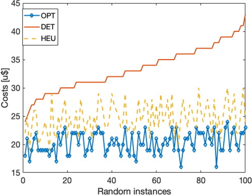
Figure 4. Decomposition of vehicle and walking costs for (a) the optimal algorithm and (b) the heuristic, when applied over 100 random graphs, which are ordered in the x-axis according to the cost of the DET algorithm.
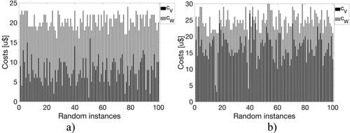
Table 1. Comparison of the three algorithms.
Table 2. Ratios (dimensionless) between walking and vehicle costs for HEU and OPT.
reveals the mean, maximum, and minimum values reached by the vectors that contain the quotients between the costs of the respective pairs of algorithms. The first row shows that OPT saves more than a third of total costs on average, and can save more than half: reducing detours via requesting users to walk can be a crucial way to improve ridesharing systems. Regarding HEU, its performance depends heavily on the graph, as it can be as good as OPT or as bad as DET.
looks deeper into the performances of OPT () and HEU (), by decomposing their costs in vehicle costs and walking costs. As apparent, in most instances vehicle costs exceed walking costs for HEU (black columns are taller than gray columns), whereas the contrary occurs for OPT, which can be interpreted by analyzing the two main characteristics that make HEU a heuristic:
Recalling that when HEU searches for the stop associated to a request
The limited future memory of HEU implies that the route it chooses does not take into account future requests in a perfect way, so when solving the tradeoff between walking time for a current user and vehicle’s time for all the future ones, the latter is underestimated and the tradeoff is inclined toward reducing walking.
synthesizes this information and confirms that both methods present quite different costs’ decomposition. OPT is much more stable, as the ratio between vehicle’s and walking costs do not change as much as in HEU.
Comparison of the algorithms over a simplified transport network
To mimic the context in which these algorithms are required, we now create a simple on-demand transport network and study the solutions that emerge when they are applied. We consider a 10 × 10 grid, in which there are three types of street: slow (20 km/h), mid-speed (30 km/h) and fast (40 km/h). Slow and fast streets are bidirectional, unlike mid-speed ones which are one-way. The vehicle departs from one extreme of the grid and needs to serve ten random requests
To simulate the fact that the systems get updated when new requests arrive, we will assume that at every point the vehicle only knows in advance the following four requests (or all the remaining requests, when they are fewer than four). Algorithms are modified as follows to account for this incomplete information:
DET always goes to the closest request within the following 4. For a proper comparison, the resulting route
OPT is repeatedly applied over the following 4 nodes in
HEU does not need to be modified, as its future memory is lower than 4.
shows arcs’ costs, whose calculations are explained in Appendix B. show the network () and requests (). The width and color of the edges represent the type of street: red (slow), gray (mid-speed) and brown (fast). Arrows show if streets are one-way or two-ways. In , the red node represents the starting point of the vehicle, and the green nodes the requests
Figure 5. The network (a) and the requests (b). Red arcs are slow, gray are mid-speed and brown are fast. Green nodes represent the requests, and the red node is the starting place.
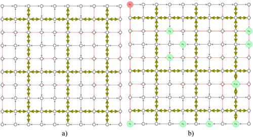
Table 3. Costs of arcs in the transport network example.
show the route generated by each of the algorithms: DET (), OPT (), and HEU (). To prevent curves from overlapping, routes’ figures are divided into two halves (before and after visiting the 5th stop). Note that all three algorithms stop in the exact fifth request, such that we can compare each half separately. Requests are shown in green and stops in purple; when they coincide in OPT or HEU, we use light blue.
Figure 6. Emerging routes when applying DET (a), OPT (b), and HEU (c).
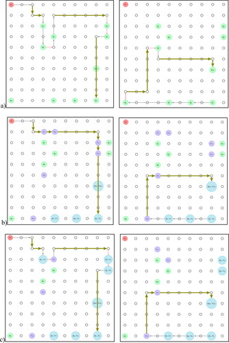
The first half of the trips (left column in ) is quite illustrative of the different solutions provided by these algorithms. DET requires using all kinds of streets, including the slow ones. The opposite happens with OPT, which uses almost only fast streets; the only exception occurs at the beginning of the route because the initial node does not have incident fast streets. Moreover, it reduces the number of arcs toured by avoiding the detour between the first and second requests. HEU’s outcome is some intermediate solution: it makes a detour between the first and second requests, but this detour is smaller than DET’s one. After the second stop, it imitates the same path followed by DET, including another detour that prevents passengers of the third and fourth requests from walking; OPT avoids this detour.
The second half of the trips (right column in ) shows exact coincidence between OPT and HEU: their path uses one mid-speed street, which is justified because there are four requests located over that street; afterward, they only use fast streets. DET adds two detours, to visit the eighth and ninth requests, which forces the route to use two slow arcs.
As a synthesis, show that OPT operates very differently from DET, taking advantage of the flexibility induced by the chance of walking, which creates shorter routes by using fewer and faster arcs. HEU sometimes behaves as DET (when going from the second to the fifth requests), sometimes as OPT (after the fifth request) and sometimes as an intermediate solution (before the second request). shows the cost of each algorithm. Although OPT is better than HEU, the difference between the latter and DET is even larger, showing that using HEU is a sound strategy over transport networks. More than one quarter of in-vehicle costs can be saved when long detours are avoided with either HEU or OPT. Moreover, HEU took 0.0093 [sec] and OPT required 0.24 [sec]. There is a huge improvement in running times at a little cost.
Table 4. Walking and in-vehicle costs per method over the simplified transport network.
These results are robust. If we repeat the same experiment 100 times, HEU is on average 19% less costly than DET, and only 5% costlier than OPT. As a final remark, we also analyzed what happens if OPT is calculated knowing the whole ten requests in advance (rather than only four). In the example explained in this section, the result does not change, and the same happens 84 times in 100 repetitions of the experiment, while in the most extreme case only 2.6% of the costs are saved: there is no need of long future memory when working over transport networks.
Comparison of the algorithms over a real-life case
In “Comparison of the algorithms over a simplified transport network,” we showed that running OPT could take 24 times more than HEU; nevertheless, as they were applied over a small example, both procedures required reasonable times. What happens if we make a similar comparison over a large real-life network? And how would total costs compare?
To answer this question, we test the algorithms over a graph that represents Manhattan, in which each edges are the real streets and nodes are corners or dead-ends. This graph contains 4,092 nodes and 9,451 edges, and it has been used previously by Alonso-Mora et al. (Citation2017) and by Fielbaum et al. (Citation2021) to test ridesharing algorithms. Walking times are proportional to the distance, while vehicle times are considered as twice the real ones, to account for users traveling in the vehicle or waiting for it. We compute 50 rides of a vehicle that starts in a random node and receives four random requests.
As shown in , conclusions with respect to costs are similar to was stated in “Comparison of the algorithms over a simplified transport network,” whereas the differences regarding computational times are much higher. Let us explain and discuss these results further:
Figure 7. Comparison of the results obtained by OPT and HEU when solving random instances over Manhattan, (a) Ratio between total costs, and (b) Ratio between computational times. In both cases OPT is in the numerator and HEU in the denominator. Both figures are sorted in increasing order.
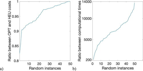
When HEU is executed, the controller of the system needs to execute just one step at a time, because the next step can be calculated after the vehicle has already moved (which is an advantage of using limited memory). Therefore, computational times are computed just considering one step, and they lay in the range of milliseconds, i.e., they do not increase with the scale of the network, which is a consequence of performing local searches.
On the other hand, the complexity of OPT is proportional to
) reveals contradictory situations. It is true that in most instances, HEU increases costs in less than 5%, reaching the optimal solution in some occasions. However, there might be specific conditions that extends the difference among the two methods to almost 20%.
Taking everything into account, it is better to use OPT when possible, but HEU provides a good alternative when OPT is too slow, which depends largely on the computational power. For instance, Alonso-Mora et al. (Citation2017) decide which requests assign to each vehicle each 30 [sec]. For a single vehicle, it might be possible to spend some seconds to determine its exact route; however, when thousands of vehicles are managed simultaneously, this is no longer possible and HEU should be chosen, unless there is plenty of computational power (for instance, each vehicle could compute its own route independently).
Conclusions and future research
In this paper, we have studied the problem of finding the optimal route of a shared vehicle, assuming that users can walk from their origins to (or to their destinations from) a different node where they meet (leave) the vehicle. Considering an exogenous order in which to fulfill the requests, we have shown that this is a polynomial problem, providing the respective algorithm.
In order to further reduce the required computational time, we proposed a heuristic with limited future memory. We compared these two algorithms and the one that visits the exact requests, by applying them over random graphs, a simplified transport network and a real-life case, showing that shortening the detours (with the optimal algorithm or with the heuristic) improves the results.
As we provide two suitable algorithms (the optimal one and the heuristic), it is worth discussing in detail the comparison among them. The heuristic can run hundreds of times faster when solving real-life instances. However, it can increase the costs up to 20%, a difference that may justify the extra time if this is compatible with operating the vehicles. How to solve this tradeoff will depend on the specific characteristics of the mobility system. Moreover, some intermediate solutions might be built by extending the so-called future memory of the heuristic. Any extension should keep the local searches utilized by the heuristic studied here, to prevent looking (repeatedly) at all the nodes in the graph.
From a practical point of view, we can identify at least two situations in which it is possible to utilize the optimal algorithm, that requires a few seconds to optimize the route of each vehicle. First, if the problem is not solved online but in advance (for instance, the night before executing the trips); in this case, optimizing the routes of thousands of vehicles would be feasible, as the process would require some hours. Second, if the routes can be computed in a distributed fashion, e.g., if each vehicle carries its own computer, so that only some seconds are required; the fact that the route of each vehicle can be computed independently is a virtue of both algorithms. On the other hand, if the calculations are centrally computed and the system works online, then the optimal algorithm is too slow and the heuristic is required.
We have shown that there might be very significant savings when optimizing the route instead of following a door-to-door scheme. The large magnitude of these savings is crucial, because it implies that it is possible to distribute such savings in a way that all the involved agents end up in a better situation. In other words: one of the central conclusions of this paper is that requiring some users to walk can be beneficial to everybody and help making these emerging mobility systems to succeed. Moreover, avoiding detours can be a strategic decision when expanding on-demand systems in order to make them part of the public transport network (as studied by Hrnčíř et al. (Citation2015) and Mounce et al. (Citation2018)), when improving the so-called MaaS systems (Hensher, Citation2017), and for carpooling systems in which different private users share the vehicle of one of them (Li et al., Citation2020; Tamannaei & Irandoost, Citation2019). It is worth recalling that the results and methods proposed here can be applied to any of the ridesharing systems that have emerged recently in the literature.
There are several promising avenues to pursue in future research. When analyzing the competitive ratio of this problem, the degree of connectivity of the graph seemed to be critical; transport networks are usually very well connected, as there are many different paths for each origin-destination pair: is it possible to obtain more promising results regarding the competitive ratio if more hypotheses with respect to the topology of the graph are assumed? Including some constraints on the walking times, as well as the chance that some users might be late (Hyland & Mahmassani, Citation2020; Kucharski et al., Citation2020), could make a more realistic model.
Acknowledgments
The author wishes to thank Víctor Verdugo and Gonzalo Muñoz, both from Universidad de O’Higgins, for their valuable comments that helped to improve this paper.
Disclosure statement
No potential conflict of interest was reported by the author(s).
Notes
1 Some authors define “sharing” as different users riding the same vehicle but at different times. This difference has significant impacts over the whole transport systems: Santi et al. (Citation2014), for instance, show that sharing taxis in New York would reduce the vehicles-kilometer traveled by this mode in about 40%.
2 There are a few real-life shared systems in which passengers are requested to walk. Uber Express Pool is already working in some American cities, although it requires that all users are gathered in the same meeting point. Many airports (Sidney, Melbourne and Madrid are some examples) have created specific spots where a passenger has to walk to meet his/her (possibly non-shared) cab. These examples, however, are very incipient, and the underlying optimization processes do not always pursue social optimum criteria.
3 As the order of the requests is fixed, the times in which requests are visited cannot change much, which is why space windows are more significant than the more traditional time windows in this scheme.
4 Classical Dijkstra’s algorithm could also be used, over a modified graph that contains the root and copies of each vertex. If is an arc in the original graph, then is an arc in the modified graph, with cost . The complexity of original Dijkstra is , that would become , which is worse than the algorithm described in the main text.
5 Moreover, papers that do model these systems usually obtain numerical results rather than analytical expressions (as Alonso-Mora et al., Citation2017; Fagnant & Kockelman, Citation2018; Martinez & Crist, Citation2016).
6 This assumes that vehicles arrive at constant headways; otherwise, a larger number replaces the ½.
References
- Alonso-Mora, J., Samaranayake, S., Wallar, A., Frazzoli, E., & Rus, D. (2017). On-demand high-capacity ride-sharing via dynamic trip-vehicle assignment. Proceedings of the National Academy of Sciences of the United States of America, 114(3), 462–467. https://doi.org/https://doi.org/10.1073/pnas.1611675114
- Badia, H., Estrada, M., & Robuste, F. (2014). Competitive transit network design in cities with radial street patterns. Transportation Research Part B: Methodological, 59, 161–181. https://doi.org/https://doi.org/10.1016/j.trb.2013.11.006
- Borodin, A. (1992). Can competitive analysis be made competitive? [Paper presentation]. Proceedings of the 1992 Conference of the Centre for Advanced Studies on Collaborative Research (Vol. 1, pp. 359–367). IBM Press.
- Borodin, A., Linial, N., & Saks, M. (1992). An optimal on-line algorithm for metrical task system. Journal of the ACM, 39(4), 745–763. https://doi.org/https://doi.org/10.1145/146585.146588
- Carlsson, J. G., & Song, S. (2018). Coordinated logistics with a truck and a drone. Management Science, 64(9), 4052–4069. https://doi.org/https://doi.org/10.1287/mnsc.2017.2824
- Chang, S., & Schonfeld, P. (1991). Multiple period optimization of bus transit systems. Transportation Research Part B: Methodological, 25(6), 453–478. https://doi.org/https://doi.org/10.1016/0191-2615(91)90038-K
- Daganzo, C. F. (1984). Checkpoint dial-a-ride systems. Transportation Research Part B: Methodological, 18(4-5), 315–327. https://doi.org/https://doi.org/10.1016/0191-2615(84)90014-6
- Daganzo, C. F. (2010). Structure of competitive transit networks. Transportation Research Part B: Methodological, 44(4), 434–446. https://doi.org/https://doi.org/10.1016/j.trb.2009.11.001
- Fagnant, D., & Kockelman, K. (2018). Dynamic ride-sharing and fleet sizing for a system of shared autonomous vehicles in Austin, Texas. Transportation, 45(1), 143–158. https://doi.org/https://doi.org/10.1007/s11116-016-9729-z
- Fielbaum, A. (2020). Strategic public transport design using autonomous vehicles and other new technologies. International Journal of Intelligent Transportation Systems Research, 18(2), 183–191. https://doi.org/https://doi.org/10.1007/s13177-019-00190-5
- Fielbaum, A., Bai, X., & Alonso-Mora, J. (2021). On-demand ridesharing with optimized pick-up anddrop-off walking locations. Transportation Research Part C: Emerging Technologies, 126, 103061.
- Foschini, L., Hershberger, J., & Suri, S. (2014). On the complexity of time-dependent shortest paths. Algorithmica, 68(4), 1075–1097. https://doi.org/https://doi.org/10.1007/s00453-012-9714-7
- Hensher, D. (2017). Future bus transport contracts under a mobility as a service (MaaS) regime in the digital age: Are they likely to change? Transportation Research Part A: Policy and Practice, 98, 86–96. https://doi.org/https://doi.org/10.1016/j.tra.2017.02.006
- Hrnčíř, J., Rovatsos, M., & Jakob, M. (2015). Ridesharing on timetabled transport services: A multiagent planning approach. Journal of Intelligent Transportation Systems, 19(1), 89–105. https://doi.org/https://doi.org/10.1080/15472450.2014.941759
- Hurdle, V. F. (1973). Minimum cost locations for parallel public transit lines. Transportation Science, 7(4), 340–350. https://doi.org/https://doi.org/10.1287/trsc.7.4.340
- Hyland, M., & Mahmassani, H. (2020). Operational benefits and challenges of shared-ride automated mobility-on-demand services. Transportation Research Part A: Policy and Practice, 134, 251–270. https://doi.org/https://doi.org/10.1016/j.tra.2020.02.017
- Jansson, J. O. (1980). A simple bus line model for optimisation of service frequency and bus size. Journal of Transport Economics and Policy, 14(1), 53–80.
- Jara-Díaz, S., & Gschwender, A. (2009). The effect of financial constraints on the optimal design of public transport services. Transportation, 36(1), 65–75. https://doi.org/https://doi.org/10.1007/s11116-008-9182-8
- Jaw, J., Odoni, A., Psaraftis, H., & Wilson, N. (1986). A heuristic algorithm for the multi-vehicle advance request dial-a-ride problem with time windows. Transportation Research Part B: Methodological, 20(3), 243–257. https://doi.org/https://doi.org/10.1016/0191-2615(86)90020-2
- Kocur, G., & Hendrickson, C. (1982). Design of local bus service with demand equilibration. Transportation Science, 16(2), 149–170. https://doi.org/https://doi.org/10.1287/trsc.16.2.149
- Kucharski, R., Fielbaum, A., Alonso-Mora, J., & Cats, O. (2020). If you are late, everyone is late: Late passenger arrival and ride-sharing systems’ performance. Transportmetrica A: Transport Science. https://doi.org/https://doi.org/10.1080/23249935.2020.1829170
- Li, M., Di, X., Liu, H. X., & Huang, H. J. (2020). A restricted path-based ridesharing user equilibrium. Journal of Intelligent Transportation Systems, 24(4), 383–403. https://doi.org/https://doi.org/10.1080/15472450.2019.1658525
- Li, R., Qin, L., Yu, J., & Mao, R. (2016). Optimal multi-meeting-point route search. IEEE Transactions on Knowledge and Data Engineering, 28(3), 770–784. https://doi.org/https://doi.org/10.1109/TKDE.2015.2492554
- Li, X., Hu, S., Fan, W., & Deng, K. (2018). Modeling an enhanced ridesharing system with meet points and time windows. PLoS One, 13(5), e0195927. https://doi.org/https://doi.org/10.1371/journal.pone.0195927
- Martinez, L., & Crist, P. (2016). Urban mobility system upgrade, how shared self-driving cars could change city traffic. OECD/ITF Forum. http://www.internationaltransportforum.org/Pub/pdf/15CPB_Self-drivingcars.pdf
- Mounce, R., Wright, S., Emele, C., Zeng, C., & Nelson, J. D. (2018). A tool to aid redesign of flexible transport services to increase efficiency in rural transport service provision. Journal of Intelligent Transportation Systems, 22(2), 175–185. https://doi.org/https://doi.org/10.1080/15472450.2017.1410062
- Mourad, A., Puchinger, J., & Chu, C. (2019). A survey of models and algorithms for optimizing shared mobility. Transportation Research Part B: Methodological, 123, 323–346. https://doi.org/https://doi.org/10.1016/j.trb.2019.02.003
- Narayanan, S., Chaniotakis, E., & Antoniou, C. (2020). Shared autonomous vehicle services: A comprehensive review. Transportation Research Part C: Emerging Technologies, 111, 255–293. https://doi.org/https://doi.org/10.1016/j.trc.2019.12.008
- Pei, M., Lin, P., Du, J., & Li, X. (2019). Operational design for a real-time flexible transit system considering passenger demand and willingness to pay. IEEE Access, 7, 180305–180315. https://doi.org/https://doi.org/10.1109/ACCESS.2019.2949246
- Psaraftis, H. (1983). An exact algorithm for the single vehicle many-to-many dial-a-ride problem with time windows. Transportation Science, 17(3), 351–357. https://doi.org/https://doi.org/10.1287/trsc.17.3.351
- Santi, P., Resta, G., Szell, M., Sobolevsky, S., Strogatz, S., & Ratti, C. (2014). Quantifying the benefits of vehicle pooling with shareability networks. Proceedings of the National Academy of Sciences of the United States of America, 111(37), 13290–13294. https://doi.org/https://doi.org/10.1073/pnas.1403657111
- Silwal, S., Gani, M. O., & Raychoudhury, V. (2019, June). A survey of taxi ride sharing system architectures [Paper presentation]. 2019 IEEE International Conference on Smart Computing (SMARTCOMP) (pp. 144–149). IEEE. https://doi.org/https://doi.org/10.1109/SMARTCOMP.2019.00044
- Sleator, D. D., & Tarjan, R. E. (1983, December). Self-adjusting binary trees [Paper presentation]. Proceedings of the Fifteenth Annual ACM Symposium on Theory of Computing (pp. 235–245). https://doi.org/https://doi.org/10.1145/800061.808752
- Stiglic, M., Agatz, N., Savelsbergh, M., & Gradisar, M. (2015). The benefits of meeting points in ride-sharing systems. Transportation Research Part B: Methodological, 82, 36–53. https://doi.org/https://doi.org/10.1016/j.trb.2015.07.025
- Tamannaei, M., & Irandoost, I. (2019). Carpooling problem: A new mathematical model, branch-and-bound, and heuristic beam search algorithm. Journal of Intelligent Transportation Systems, 23(3), 203–215. https://doi.org/https://doi.org/10.1080/15472450.2018.1484739
- Tirachini, A. (2014). The economics and engineering of bus stops: Spacing, design and congestion. Transportation Research Part A: policy and Practice, 59, 37–57. https://doi.org/https://doi.org/10.1016/j.tra.2013.10.010
- Tirachini, A., Hensher, D., & Jara-Díaz, S. (2010). Comparing operator and users costs of light rail, heavy rail and bus rapid transit over a radial public transport network. Research in Transportation Economics, 29(1), 231–242. https://doi.org/https://doi.org/10.1016/j.retrec.2010.07.029
- Tsao, M., Milojevic, D., Ruch, C., Salazar, M., Frazzoli, E., & Pavone, M. (2019, May). Model predictive control of ride-sharing autonomous mobility-on-demand systems [Paper presentation]. In 2019 International Conference on Robotics and Automation (ICRA) (pp. 6665–6671). IEEE. https://doi.org/https://doi.org/10.1109/ICRA.2019.8794194
- Wang, H., & Yang, H. (2019). Ridesourcing systems: A framework and review. Transportation Research Part B: Methodological, 129, 122–155. https://doi.org/https://doi.org/10.1016/j.trb.2019.07.009
- Wilson, N., Weissberg, R., & Hauser, J. (1976). Advanced dial-a-ride algorithms research project (No. R76-20 Final RPt.).
- Zhao, M., Yin, J., An, S., Wang, J., & Feng, D. (2018). Ridesharing problem with flexible pickup and delivery locations for app-based transportation service: Mathematical modeling and decomposition methods. Journal of Advanced Transportation, 2018, 1–21. https://doi.org/https://doi.org/10.1155/2018/6430950
- Zheng, Y., Li, W., Qiu, F., & Wei, H. (2019). The benefits of introducing meeting points into flex-route transit services. Transportation Research Part C: Emerging Technologies, 106, 98–112. https://doi.org/https://doi.org/10.1016/j.trc.2019.07.012
Appendix A:
Proof of the proposition in “Some results on the competitive ratio”
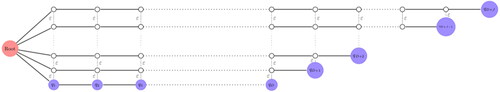
Without loss of generality, we assume that Define a graph
with
Let
be a large number (eventually, we will make
) and let
Each set
contains
nodes
which form a vehicle path (let us call it a “highway”), i.e.,
with
There are arcs between the respective nodes of consecutive paths, representing very short pedestrian bridges, i.e.,
with
The vehicle starts at the root
and the requests vector is
shows this network, with the requests in solid blue.
Figure A1. Network and requests that yield a competitive ratio larger than
If is small enough, the optimal route is taking the
-th highway, because it needs to be taken at some moment to reach the final request, and walking costs are negligible. This yields:
(9)
(9)
The first term in (9) are vehicle’s costs, the second term represents the first requests (the cost of walking toward the first highway), and the following terms come from the other requests’ walking costs. Note that only the first term will be relevant when making
What happens with the -algorithm? At the beginning, it only looks at requests that are located over the first highway, so it is going to take it. When reaching the
th request, node
enters the requests vector, which cannot be reached walking from the first highway, forcing the vehicle to go back to the root and to take the second highway. The same happens repeatedly afterward, making the vehicle tour completely all the highways from the second to the last one, yielding:
(10)
(10)
The first term in (10) is induced by going from the root to and back. The second term appears when visiting the next
stops (whose passengers need to walk to the first highway). The third term represents visiting all the next highways but the last one, whose stops are
bridges away from the respective exact requests. The last term is caused by touring the last highway, responding to
requests on the way. Rearranging:
(11)
(11)
where
is a term that does not depend on
and in which
appears only multiplying some terms, such that it is irrelevant when
It is apparent then that
which proves the proposition.
Appendix B:
Arc’s costs in “Comparison of the algorithms over a simplified transport network”
To calculate the vehicle and walking costs, we follow the guidelines of ridesharing transport systems, but without using a detailed model, such that is the sum of operators’ and users’ costs, while
depends only on users. Let us denote
the (homogenous) length of the arcs.
Explicit expressions for operators’ costs would require a detailed model for an on-demand system, which is beyond the scope of this paper. Instead, we take as reference the well-known expression for a single line in a traditional public transport system
Users’ costs increase due to the delay on their arrival times, by an amount that depends on the arc’s speed. If
Walking costs depend on the walking speed
The numeric value of the parameters is shown in Appendix C.
Appendix C:
Numeric value of the parameters
When needed, costs are taken from Fielbaum (Citation2020).
Table A1. Numeric value of the parameters.