Performance evaluation of a state-of-the-art automotive radar and corresponding modeling approaches based on a large labeled dataset

Abstract

Radar is a key sensor to achieve a reliable environment perception for advanced driver assistance system and automated driving (ADAS/AD) functions. Reducing the development efforts for ADAS functions and eventually enabling AD functions demands the extension of conventional physical test drives with simulations in virtual test environments. In such a virtual test environment, the physical radar unit is replaced by a virtual radar model. Driving datasets, such as the nuScenes dataset, containing large amounts of annotated sensor measurements, help understand sensor capabilities and play an important role in sensor modeling. This article includes a thorough analysis of the radar data available in the nuScenes dataset. Radar properties, such as detection thresholds, and detection probabilities depending on object, environment, and radar parameters, as well as object properties, such as reflection behavior depending on object type, are investigated quantitatively. The overall detection probability of the considered radar (Continental ARS-408-21) was found to be 27.81%. Four radar models on object level with different complexity levels and different parametrisation requirements are presented: a simple RCS-based radar model with an accuracy of 51%, a linear SVC model with an accuracy of 70%, a Random Forest model with an accuracy of 83%, and a Gradient Boost model with an accuracy of 86%. The feature importance analysis of the machine learning algorithms revealed that object class, object size, and object visibility are the most important parameters for the presented radar models. In contrast, daytime and weather conditions seem to have only minor influence on the modeling results.

Keywords:

• automotive radar
• nuScenes
• sensor model
• virtual test

1. Introduction

More than 1.35 million people die in road traffic crashes each year, and up to 50 million get injured or disabled (World Health Organisation (WHO), 2018). Advanced driver assistance system, and automated driving (ADAS/AD) functions are meant to play an important role in improving safety both for vehicle passengers and vulnerable road users, such as pedestrians (Anderson et al., 2016; Fagnant & Kockelman, 2015; Watzenig & Horn, 2016).

Radar is a key sensor to achieve a reliable environment perception for ADAS/AD functions (Marti et al., 2019). Modern automotive radar (such as the one addressed in this study) typically operate at 77 GHz (Ramasubramanian & Ramaiah, 2018) and apply Frequency-Modulated Continuous Wave (FMCW) technologies for relative distance and velocity estimation (Patole et al., 2017) and digital beamforming to control the direction of the emitted wave (Hasch, 2015). Automotive radar are considered very robust against disturbing atmospheric and environmental factors (Marti et al., 2019), even though some small effects caused by heavy rain (Hasirlioglu et al., 2016; Hassen, 2007) and water droplets, ice, or dirt particles on the radome (Arage et al., 2006; Eltayeb et al., 2018) have been reported.

Despite the radar’s importance for automotive applications, there has been no study conducted so far, that investigates the performance of current state-of-the-art automotive radars based on a dataset that has been collected on public roads and is large enough to be considered representative for most real life scenarios.

1.1. Virtual testing of ADAS/AD functions

Development, testing, and validation of ADAS/AD functions represent major challenges for today’s SAE Level-2 (SAE, 2018) vehicles and the effort will increase significantly for SAE Level-3+ vehicles. In particular, AD vehicles would have to be driven hundreds of millions of kilometers to demonstrate their reliability (Kalra & Paddock, 2016). To reduce the development effort for ADAS functions and to eventually enable AD functions demands the extension of physical test drives with simulations in virtual test environments (Hakuli & Krug, 2015; Watzenig & Horn, 2016).

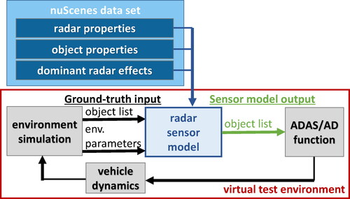
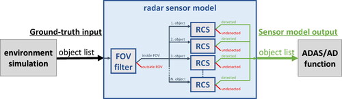
In a virtual test environment, a radar is simulated by a radar sensor model. The flow chart in Figure 1 illustrates the data flow of a virtual test environment for ADAS/AD functions, including the presented object-based radar model. An environment simulation, e.g., Vires VTD (VIRES, 2019), IPG CarMaker (IPG, 2019), CARLA (Dosovitskiy et al., 2017), or AirSim (Shah et al., 2017), provides the test scenario and forwards the true state of the environment, called ground-truth, to the radar model. The radar model modifies the ground-truth according to the sensing capabilities of the considered radar. The radar model output is then fed into the ADAS/AD function under test. A promising approach to standardize the interfaces, called Open Simulation Interface, is currently under development (Hanke et al., 2017).

Figure 1. Radar sensor model embedded into a virtual test environment including environment simulation, object recognition, ADAS/AD function and vehicle dynamics. Radar and object properties, as well as implemented sensor effects in the radar model are derived and parametrized using the nuScenes dataset.

1.2. Previous work on automotive radar modeling

Previous work on automotive radar modeling includes both generic, i.e., applicable for any perception sensor, and radar specific approaches (Schlager et al., 2020).

Examples for generic sensor models that can simulate automotive radar are Hanke et al. (2015); Hirsenkorn et al. (2015); Muckenhuber et al. (2019); Stolz and Nestlinger (2018). Hanke et al. (2015) suggest to modify the ground-truth object list sequentially in a number of modules, each representing a specific sensor characteristic or environmental condition. Hirsenkorn et al. (2015) reproduce sensor behavior implicitly using probability density functions (PDF) based on kernel density estimations. Muckenhuber et al. (2019) introduce a generic sensor model that takes coverage, object dependent field of views, and false negative/false positive detections into account.

Examples for sensor models specifically designed for radar applications include Bernsteiner et al. (2015); Buehren and Yang (2006a, 2006b, 2007a, 2007b, 2007c, 2007d); Cao et al. (2015, Cao, 2017); Danielsson (2010); Hammarstrand et al. (2012a, 2012b); Hirsenkorn et al. (2017); Maier et al. (2018a, 2018b); Mesow (2006); Schuler (2007); Schuler et al. (2008); Wheeler et al. (2017). Mesow (2006) reduces the complexity of radar simulations by implementing radar target abstractions, i.e., statistical description of the vehicle radar cross section (RCS) and representation of vehicles by point reflectors. Schuler (2007); Schuler et al. (2008) apply ray-tracing simulations and a greedy algorithm to represent objects by a small number of virtual scattering centers. The radar model from Bernsteiner et al. (2015) provides detection probabilities depending on antenna pattern and a weather parameter. Wheeler et al. (2017) train a deep learning neural network to build a conditional PDF that connects the scene (objects, road infrastructure, weather, etc.) with radar raw data (power return field). Buehren and Yang (2006a, 2006b, 2007a, 2007b, 2007c, 2007d) present a radar simulation concept that includes target abstraction and sensor specific characteristics. Each object is converted into point scattering centers and plane reflectors. Based on the arrangement of sensors, scatterers, and reflectors, a realistic radar target list is provided. Danielsson (2010); Hammarstrand et al. (2012a, 2012b) replace the deterministic amplitude used by Buehren and Yang (2006a, 2006b, 2007a, 2007b, 2007c, 2007d) with a stochastic amplitude to allow random clustering. Cao et al. (2015, Cao, 2017) describe objects in the far range by their RCS and use wave propagation for the short-range. Hirsenkorn et al. (2017); Maier et al. (2018a, 2018b) perform ray tracing to simulate wave propagation and reflections in the scene.

The above discussed radar models have only been tested in a few scenarios, but not yet evaluated using a labeled dataset large enough to be considered representative for most real life scenarios. This implies that the overall model performance of current state-of-the-art radar models for automotive applications is still open to assess.

1.3. Datasets for sensor modeling

Datasets containing large amounts of sensor measurements play an important role in assessing sensor performance and sensor modeling. They allow us to find and extract dominant sensor effects and to parametrize these effects in a sensor model.

Many driving datasets are publicly available (Kang et al., 2019). However, most datasets address either solely camera applications (Cordts et al., 2016; Huang et al., 2018, 2019; Xu et al., 2017; Yu et al., 2018) or provide a combination of lidar and camera data (Geiger et al., 2012, 2013; Sun et al., 2019). Only very few datasets include radar measurements (Caesar et al., 2019; Kang et al., 2019; Meyer & Kuschk, 2019). The nuScenes dataset (Caesar et al., 2019) is currently the largest, open access, labeled dataset on public roads that includes radar measurements. To our knowledge, no automotive radar model has yet been published that is derived from a large publicly available driving datasets.

1.4. Scope of this work

Listed below are the addressed research questions and the corresponding contributions of this work:

• What is the overall performance of a state-of-the-art automotive radar sensor on public roads when considering a very large amount of different scenarios including challenging boundary conditions such as urban areas?

  We present a qualitative and quantitative analysis of the radar data available in the nuScenes dataset and investigate radar properties, such as detection thresholds and detection probabilities, as well as object properties, such as reflection behaviour.

• Which level of radar model accuracy can be reached by different model complexity levels, i.e., which level of detail is required to reach a certain radar model accuracy?

  We built two types of radar models on object level with different complexity levels and parametrisation requirements. The RCS-based model represents an ideal sensor. In the system development process of an ADAS/AD function, ideal sensor models are used in the early development stages, e.g. for requirement specification and architecture design. The ML(machine learning)-based models provide a more realistic and challenging input for the ADAS/AD function under test. These models may therefore be used in later stages of the system development process, e.g. for system testing and validation.

• What are the dominant effects that cause an object to be detected or undetected by a radar, i.e., which radar model input parameters are important and which can be neglected?

  We calculate additional object parameters, such as visibility and number of occluders, and evaluate detection probabilities depending on object and environmental parameters. To better understand which combination of input parameters are favourable for a radar model, we perform feature importance analysis on the ML-based models.

1.5. Structure of the article

Section 2 introduces the nuScenes dataset. Sections 3-8 present the analysis of the radar data incl. radar detection thresholds, precision of the radar clusters, a simplified object classification schema, object reflection properties, additionally calculated object parameters, and radar detection probabilities. Sections 9-12 introduce an RCS-based and three ML-based radar models including performance evaluation. Section 13 completes with a conclusion and an outlook on future work.

2. Nuscenes dataset

The nuScenes dataset (Caesar et al., 2019) is the first publicly available large-scale dataset that provides data from the entire sensor suite of an autonomous vehicle, i.e., camera, lidar, and radar. The full nuScenes dataset was released in March 2019 and consists of 1000 driving scenes in Boston and Singapore. Each scene is 20 seconds long and manually selected to comprise diverse driving maneuvers, traffic situations, and unexpected behaviors. The dataset includes 1.4 M camera images, 390k lidar sweeps, 1.4 M radar sweeps, and 1.4 M object bounding boxes in 40k keyframes.

Two Renault Zoe cars with identical sensor layouts, i.e., six cameras (Basler acA1600-60gc), one lidar (Velodyne HDL32E), and five radars (Continental ARS 408-21), were used for data collection. The cameras have 12 Hz capture frequency, apply auto exposure limited to maximum 20 ms, and use a $1/1.8″$ CMOS sensor with 1600 × 1200 resolution. The images are cropped to a region of interest with 1600 × 900 resolution to reduce the processing effort. The lidar has 20 Hz capture frequency, ${360}^{°}$ horizontal and ${10}^{°}$ to $-{30}^{°}$ vertical field of view, 32 channels (i.e., vertical pixel resolution), a maximum range of around 80 − 100 m with an accuracy of 2 cm, and is capable of recording up to 1.39 M points per second. The radar has 13 Hz capture frequency, and measures distance and velocity up to a range of 250 m. To achieve a good data alignment between the three sensor types, camera and radar are triggered when the lidar sweeps across the center of the camera’s and radar’s FOV, respectively. Since camera and radar run at 12 Hz and 13 Hz, and the lidar at 20 Hz, the 12 camera and the 13 radar exposures are spread as evenly as possible across the 20 lidar scans.

All 1000 driving scenes of the nuScenes dataset are labeled at keyframes at 2 Hz by human experts using all available sensor data. Labeling data is currently only available for 850 scenes, since the annotations of the remaining 150 scenes are withheld due to an ongoing object detection challenge. This study is based on the available 850 scenes, which include a total of 1 166 187 labeled objects. The data annotation includes labeling of 23 different object classes with accurate 3 D bounding boxes and additional attributes such as visibility, activity, and pose. The following object parameters provided in the nuScenes dataset are used in this paper:

• (X, Y, Z)… position of object

• (L, W, H)… length, width, height of object

• (Yaw, Roll, Pitch)… yaw, roll, pitch angle of object

• TYP… object class

Based on the consecutive object positions (X, Y, Z) and the time step between the data annotations, we calculate the absolute object velocity V relative to the surrounding environment and add this velocity information to the object parameters.

In addition to the object parameters, human experts annotated the state of the environment for each keyframe. The following environmental condition parameters provided in the nuScenes dataset are used in this paper:

• DT… daytime [day/night]

• W… weather condition [sun/rain]

The nuScenes vehicles are equipped with five equal radar sensors pointing in different (partly overlapping) directions (front, front right, front left, back right, back left). The used radar type is a Continental ARS-408-21 (Continental, 2016, 2017; Liebske, 2019), which operates in the frequency domain 76 − 77 GHz and measures distance and velocity independently in one cycle using FMCW (Frequency Modulated Continuous Wave). The FOV of the used radar (black dashed line in Figure 2) is split into two far range areas (range $r=250 m$ at horizontal opening angle $\varphi =\pm 4^{°}$ and $r=160 m$ at $\varphi =\pm 9^{°}$) and two near range areas ($r=70 m$ at $\varphi =\pm {40}^{°}$ and $r=20 m$ at $\varphi =\pm {60}^{°}$). Radar data is collected in the cluster mode, which means that the reflected signals are processed in multiple steps before made available in form of clusters. Clusters represent radar detections with information like position, velocity, and signal strength. They are newly evaluated every cycle, unlike objects, which have a history and consist of tracked clusters. The nuScenes ’devkit’ provides the option to choose the number of radar sweeps around the keyframe, by adding intermediate sweeps between the keyframes. For the following data analysis, only one sweep (closest to the keyframe) was selected. The following radar cluster parameters provided in the nuScenes dataset are used in this paper:

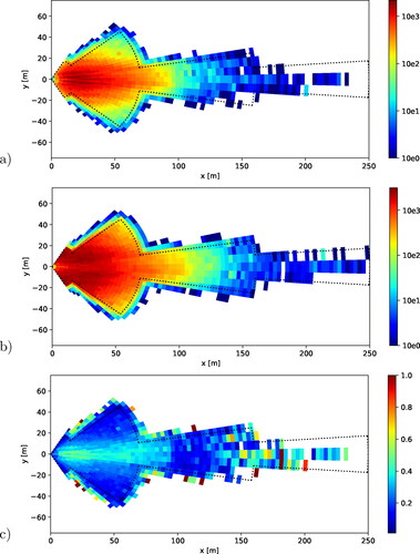
Figure 2. (a) Amount of radar cluster points received in each cell and (b) minimum radar cross section value RCS_min [dBsm] that was received in the respective cell. The radar’s FOV according to (Continental, 2016, 2017) is depicted with a black dashed line.

• (x, y, z)… position of radar cluster

• RCS… radar cross section of radar cluster

3. Radar detection threshold

The radar measurements, i.e., the radar cluster parameters, in the nuScenes dataset allow to derive the RCS (radar cross section) detection threshold of the considered radar type depending on range r and viewing angle θ.

All radar cluster points received by the five radar sensors are collected and mapped in a polar coordinate system (with r and θ being the distance and angle from the respective radar) on a grid with cell resolution $\Delta r=3.125 m$ and $\Delta \theta =3{ }^{°}.$ The minimum radar cross section value RCS_min detected in each cell is then considered as the radar detection threshold. Figure 2 (a) depicts the amount of radar cluster points received in each cell and Figure 2 (b) depicts the minimum radar cross section value RCS_min that was received in the respective cell.

Figure 2 (b) shows that the radar detection threshold is typically around 0 dBsm within the defined FOV. Only in the very close proximity ($r<5 m$), the RCS_min values are distinct lower around −5 dBsm, and at distances between $r=40-70 m$ at high incidence angles ($\theta =25-{40}^{°}$), the RCS_min values are distinct higher (5 − 10 dBsm).

4. Precision of radar clusters

The radar clusters and the object bounding boxes in the nuScenes dataset allow to assess how many of the radar detections can be associated with a labeled object and how many must be considered as clutter, i.e. unwanted echos in the radar signal, or false positive detections. To link the radar clusters to the labeled objects, the following steps are performed for each dataset collected by the five radar sensors:

(4.1) Coordinate transformation of all object bounding boxes into the coordinate system of the respective radar.

(4.2) All radar cluster points that are found in the volume of an extended (+20% length, +20% width and +20% height) object bounding box are assigned to the respective object. Nota bene: in a few cases this causes a single radar cluster to be assigned to two different objects. Altogether 0.22% (i.e. 14 808) of all radar cluster points were assigned to two different objects.

(4.3) Each radar cluster that is assigned to an object is considered as TP_cluster (true positive) and each cluster that could not be assigned to any object is considered as FP_cluster (false positive).

Note that FP_cluster detections can also arise from real infrastructure elements, such as buildings, bridges, or tunnels. These infrastructure elements are not labeled in the nuScenes dataset and are typically also not within the scope of an automotive radar. They are therefore considered as FP_cluster detections. Applying the above described procedure, the total amount of 6 687 276 radar cluster points in the nuScenes dataset, can be divided into 758 678 TP_cluster detections and 5 928 598 FP_cluster detections. The radar cluster precision Precision_cluster can be derived using the following equation: (1) $$\mathit{Precisio}{n}_{\mathit{cluster}}=\frac{T{P}_{\mathit{cluster}}}{T{P}_{\mathit{cluster}}+F{P}_{\mathit{cluster}}}$$(1)

This leads to an overall precision of the radar cluster points in the nuScenes dataset of $\mathit{Precisio}{n}_{\mathit{cluster}}=11.35 \%,$ meaning that 11.35% of all radar clusters could be assigned to a labeled object.

5. Simplified classification schema

The nuScenes dataset provides a discrimination between 23 object classes. To increase the number of observed targets per object class, classes that appear similar to radar were grouped together in a simplified classification schema with five object classes (Table 1). This simplified classification schema is used in the following.

Table 1. Simplified classification schema with 5 object classes and nuScenes classification schema with 23 object classes.

Simplified classification	nuScenes classification
static object	barrier; debris; pushable/pullable; bicycle rack; traffic cone
pedestrian	animal; child; adult; construction worker; police officer
bike	bicycle; motorcycle; stroller; wheelchair; personal mobility
normal vehicle	car; ambulance; police
big vehicle	bendy bus; rigid bus; construction vehicle; trailer; truck

6. Radar reflection properties of objects

The object and radar parameters in the nuScenes dataset allow evaluating the reflection properties of different object classes. Whenever an object can be assigned one or more radar cluster points, two additional parameters are added to the object: the number of clusters NC detected in the proximity of the object, and the radar cross section RCS of the object. Note that the RCS value assigned to the object is solely based on the Continental ARS-408-21 measurement and therefore includes the weighting by the signal processing inside the Continental ARS-408-21. This is favorable for evaluating and modeling the Continental ARS-408-21 performance, but limits the applicability of the calculated RCS values to estimate the actual RCS of the respective object classes. To evaluate the reflection properties of objects, the following steps are performed for each dataset collected by the five radar sensors:

(6.1)Coordinate transformation of all object bounding boxes into the coordinate system of the respective radar.

(6.2)All radar cluster points that are found in the volume of an extended (+20% length, +20% width and +20% height) object bounding box are assigned to the respective object.

(6.3)Each object that has assigned one or more cluster points is considered as detected by the radar.

(6.4)The yaw angle ψ relative to the line of sight between respective radar and object center is calculated for each detected object.

(6.5)The number of clusters NC found in the extended bounding box is calculated for each detected object.

(6.6)The sum of the RCS values of all cluster points assigned to the corresponding object is calculated for each detected object. This sum is in the following referred to as the RCS of the object.

The analysis in this Section is based solely on detected objects and neglects undetected objects. Figure 3 depicts the distribution of number of cluster points NC for each object class. A single cluster per object is the most likely case for all object classes. Smaller object classes have typically fewer cluster points associated (up to 4 cluster points for pedestrians and up to 8 cluster points for bikes), whereas larger object classes (normal and big vehicles) can have up to 15-20 associated cluster points. Figure 4 depicts the RCS distribution incl. mean RCS values for each object class. The average RCS values of the respective object classes are shown in Table 2. Smaller object classes, such as pedestrian and bike, have a value of around 2 − 3 dBsm, whereas normal vehicles have an average RCS value of around 10 dBsm and large vehicles of around 20 dBsm. Figure 5 depicts RCS mean, standard deviation, minimum, and maximum values for each object class depending on yaw angle ψ.

Figure 3. Distribution of number of cluster points NC for each object class.

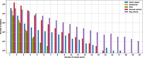
Figure 4. RCS distribution incl. mean RCS values for each object class for (a) static objects, (b) pedestrians, (c) bikes, (d) normal vehicles, and (e) big vehicles.

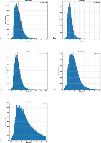
Figure 5. RCS distribution incl. number of data points for each object class depending on yaw angle ψ for (a) static objects, (b) pedestrians, (c) bikes, (d) normal vehicles, and (e) big vehicles.

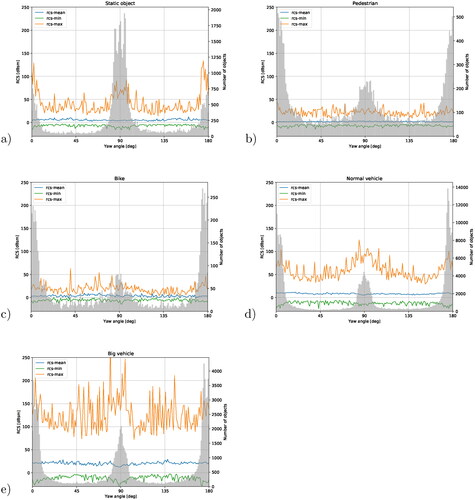
Table 2. Average RCS value of each object class.

static object	$4.81 \mathit{dBsm}$
pedestrian	$1.74 \mathit{dBsm}$
bike	$3.46 \mathit{dBsm}$
normal vehicle	$8.98 \mathit{dBsm}$
big vehicle	$19.97 \mathit{dBsm}$

7. Visibility and occlusion from radar perspective

The visibility class annotation in the nuScenes dataset is based on the panoramic view of 6 cameras and not applicable when considering the radar data, e.g., an object might have visibility class 4 (80-100% visibility) while being completely outside the radar’s FOV. To calculate visibility and occlusion parameters from the radar perspective, mounting positions, radar FOV, and object bounding boxes are used. Whenever an object is found inside the FOV of one of the five radar, two additional parameters are added to the object information: number of occluders NOCC (i.e. the number of other objects in the line of sight between respective radar and object) and relative visible area VIS[%](i.e. area not occluded by other objects). To calculate NOCC and VIS[%], the following steps are performed for each dataset collected by the five radar sensors:

(7.1)Coordinate transformation of all object bounding boxes into the coordinate system of the respective radar.

(7.2)Objects outside the respective radar’s FOV are removed.

(7.3)Computation of a boolean occlusion matrix which contains the information which object is occluding which.

(7.4)Based on the occlusion matrix, the number of occluders NOCC is calculated for each object in the radar’s FOV.

(7.5)2D polygons are constructed from the 3D object bounding boxes by using perspective projection and finding the convex hull.

(7.6)The 2D polygons are clipped with each other in an order derived from the occlusion matrix.

(7.7)Relative visible, i.e., not occluded, areas VIS[%]of the clipped polygons are calculated.

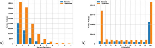
Figure 6 depicts the distributions of the number of occluders NOCC and the relative visible area VIS[%]. The following Section 8 further evaluates how the object parameters VIS and NOCC influence the detection probability of the radar.

Figure 6. Amount of detected D and undetected objects U by the radar sensors depending on (a) number of occluders NOCC and (b) relative visible area VIS resolved in 10% steps.

8. Detection probability

The object, environment, and radar parameters provided in the nuScenes dataset, as well as the added parameters V, VIS, and NOCC, allow to calculate the radar detection probability P_D and evaluate how P_D depends on range r, viewing angle θ, object class, daytime, weather condition, visibility, occlusion, and object velocity. To derive detection probabilities P_D, the following steps are performed for each dataset collected by the five radar sensors:

(8.1)Coordinate transformation of all object bounding boxes into the coordinate system of the respective radar.

(8.2)Objects outside the respective radar’s FOV are removed.

(8.3)An object is considered as detected if one or more radar cluster points can be assigned to the extended (+20% length, +20% width and +20% height) object bounding box. All remaining objects inside the radar’s FOV are considered as undetected.

(8.4)The number of detected objects D_i and the number of undetected objects U_i is calculated for the respective radar.

The final detection probability P_D (Echard, 1991) is then calculated by taking the amount of detected and undetected objects of all five radar sensors into account: (2) $$P_D=\frac{\sum _{i=1}^5{D}_i}{\sum _{i=1}^5(D_i+U_i)}=\frac{D}{D+U}$$(2)

Adding up the numbers of detected objects D_i and undetected objects U_i of the five radar sensors results in $D={\sum }_{i=1}^5{D}_i=443320$ and $U={\sum }_{i=1}^5{U}_i=1150621.$ This gives an overall detection probability $P_D=27.81 \%.$ The detection probability P_D refers to single scan detection. Note that automotive radar typically apply advanced detection algorithms taking multiple scans into account, which may increase the radar performance.

To evaluate the influence of range r and viewing angle θ on the detection capability of the radar, Figure 7 shows the amount of detected and undetected objects, and the corresponding detection probability P_D distribution on a polar coordinate grid with cell resolution $\Delta r=3.125 m$ and $\Delta \theta =3{ }^{°}.$ Note that this analysis does not require the above-mentioned removal of objects outside the radar’s FOV. This step was, therefore, not applied here. The detection probability decreases with increasing range and increasing viewing angle θ.

Figure 7. Amount of (a) detected and (b) undetected objects and (c) corresponding detection probability P_D depending on r and θ. The radar’s FOV according to (Continental, 2016, 2017) is depicted with a black dashed line.

To evaluate the influence of the object class on the detection probability P_D of the radar, Figure 8(a) depicts the amount of detected D and undetected objects U by the radar sensor depending on the object class. The detection probability of the respective object classes are 11.78% (static object), 7.75% (pedestrian), 20.74% (bike), 38.58% (normal vehicle), and 53.61% (big vehicle).

Figure 8. Amount of detected D and undetected objects U by the radar sensors depending on (a) object class and (b) environmental conditions.

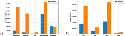
To evaluate the influence of environmental parameters on the detection probability P_D of the radar, Figure 8(b) depicts the amount of detected D and undetected objects U by the radar sensor depending on daytime and weather conditions. The detection probability is 27.98% during day time, 25.16% during the night, 27.32% in sunny weather, and 29.79% during rain.

To evaluate the influence of the relative visibility VIS[%]and the number of occluders NOCC on the detection probability P_D of the radar, Figure 6 depicts the amount of detected D and undetected objects U by the radar sensor depending on the number of occluders NOCC and the relative visible area VIS. In case NOCC = 0, i.e., no other object is in the line-of-sight between radar and target, the detection probability is around 34% and distinct higher as in cases where the NOCC value is above 1. However, even in cases where 9 other objects are standing between radar and target, the detection probability is still around 23%. Objects that are completely occluded, i.e., $\mathit{VIS}=0 \%,$ are improbable to be detected by the radar. However, occlusion values up to 80% have only a small influence on the the detection probability.

To evaluate the influence of the absolute object velocity visibility $V[m/s]$ on the detection probability P_D of the radar, Figure 9 depicts the amount of detected D and undetected objects U by the radar sensor depending on the absolute object velocity visibility $V[m/s]$ in $1 m/s$ steps. Objects that move faster than $2.5m/s$ are clearly have a distinct higher detection probability than objects that are slower or standing.

Figure 9. Amount of detected D and undetected objects U by the radar sensors depending on absolute object velocity V relative to environment.

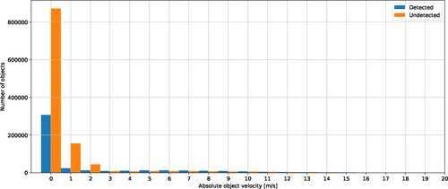
Table 3 provides the corresponding detection probabilities P_D depending on the number of occluders NOCC, the relative visible area VIS and the absolute object velocity $V[m/s].$

Table 3. Detection probabilities P_D depending on number of occluders NOCC, relative visible area VIS and absolut object velocity $V[m/s]$ relative to environment.

NOCC	PD
0	33.59 %
1	26.96 %
2	22.88 %
3	20.04 %
4	19.29 %
5	19.56 %
6	19.25 %
7	19.59 %
8	19.18 %
9	23.41 %
VIS	PD
0 %	7.26 %
10 %	26.06 %
20 %	34.08 %
30 %	37.94 %
40 %	38.14 %
50 %	36.73 %
60 %	35.77 %
70 %	33.73 %
80 %	30.82 %
90 %	28.65 %
100 %	34.28 %
$v [m/s]$	$P_D$
0-0.5	26.04 %
0.5-1.5	13.06 %
1.5-2.5	22.19 %
2.5-3.5	54.85 %
3.5-4.5	59.01 %
4.5-5.5	59.50 %
5.5-6.5	60.47 %
6.5-7.5	60.21 %
7.5-8.5	60.21 %
8.5-9.5	59.62 %
9.5-10.5	54.66 %
10.5-11.5	49.36 %
11.5-12.5	49.91 %
12.5-13.5	45.74 %
13.5-14.5	44.90 %
14.5-15.5	43.44 %
15.5-16.5	37.91 %
16.5-17.5	38.22 %
17.5-18.5	34.91 %
18.5-19.5	40.33 %

9. Radar modeling on object level

Based on the analysis of the nuScenes dataset and the Continental ARS-408-21 specification sheet, the sections above present several important aspects for radar modeling on object level (FOV specification, detection thresholds, cluster point precision, object reflection properties, detection probabilities, etc.). The possibility to implement these aspects in a new radar model depends on the information provided in the specification sheet and the availability of test data collected with the specific radar type. Depending on the purpose of the conducted virtual test, different levels of model fidelity are required. To address the question, which level of detail is required for which degree of model fidelity, two types of radar models with different complexity levels and parametrisation requirements are presented in the following. Section 10 introduces a simple radar model based on RCS detection thresholds. This model can easily be adapted to a new radar sensor without the necessity to collect large amounts of training data. Section 11 introduces more sophisticated approaches using supervised machine learning (ML) algorithms that require the collection of a representative dataset including ground-truth information.

10. RCS-based radar model

The RCS detection threshold of the radar (Figure 2), together with object reflection properties (Section 6), can be used to build a simple radar model based on RCS. In case the detection thresholds of the considered radar is provided in the specification sheet, the RCS-based radar model can be parametrized without collecting any training data. The data pipeline of the RCS-based radar model is illustrated in Figure 10 and includes the following steps:

Figure 10. Processing steps and data flow of the RCS-based radar model. The radar model removes objects outside the radar’s FOV and according to the RCS detection threshold of the radar.

1. A ground-truth object list is provided by the environment simulation.

(10.2)Objects outside the radar’s FOV are removed.

(10.3)RCS_object values are derived for all remaining objects from Table 2.

(10.4)The minimum radar cross section RCS_min for every object location is derived from Figure 2 and compared to RCS_object for the detection decision:

$RC{S}_{\mathit{object}}\ge RC{S}_{\mathit{min}}\to$ detected

$RC{S}_{\mathit{object}}<RC{S}_{\mathit{min}}\to$ undetected

(10.5)Detected objects are provided as object list to the ADAS/AD function.

11. ML-based radar models

As shown in Section 8, there are several additional factors to the RCS that have an impact on whether an object is detected by the radar or remains undetected, proposing a potential thread to the ADAS/AD vehicle. A radar model with a high fidelity level must take all major influencing factors into account while being computationally efficient enough to enable real-time capability. The radar models presented in this section aim to fulfill these two requirements by applying supervised machine learning (ML) algorithms that provide the detection decision for each individual object inside the radar’s FOV. The data pipeline of the ML-based radar models is shown in Figure 11 and include the following steps:

Figure 11. Processing steps and data flow of the ML-based radar models. The radar model removes objects outside the radar’s FOV and according to the detection decision of a ML algorithm.

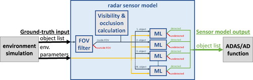
(11.1)A ground-truth object list and environment parameters are provided by the environment simulation.

(11.2)Objects outside the radar’s FOV are removed.

(11.3)NOCC and VIS values are calculated for all remaining objects.

(11.4)A ML algorithm evaluates for each object, whether the object is detected or undetected.

(11.5)Detected objects are provided as object list to the ADAS/AD function.

The core element of the presented radar model is the supervised ML algorithm, which decides whether an object is detected or undetected based on radar, object, and environmental parameters. The input and output parameters of the ML algorithm are listed in Table 4.

Table 4. ML algorithm input and output parameters.

ML algorithm input
parameter	value
object class	$[\mathit{static} \mathit{object},\mathit{pedestrian},\mathit{bike},$
	$\mathit{normal} \mathit{vehicle},\mathit{big} \mathit{vehicle}]$
object position	$(X,Y,Z)[m]$
bounding box dimensions	$(L,W,H)[m]$
bounding box orientation	$(\mathit{Yaw},\mathit{Roll},\mathit{Pitch}){[}^{°}]$
object velocity	$V[m/s]$
number of occluders	NOCC
visible area	VIS [%]
daytime	$DT[\mathit{day},\mathit{night}]$
weather condition	$W[\mathit{sun},\mathit{rain}]$
$\to$
ML algorithm output
parameter	value
object detection	[detected, undetected]

To provide a balanced dataset for training and testing of the ML algorithms, 442 891 detected and 442 891 undetected objects inside the radar’s FOV were selected randomly from the total amount of 1 593 941 objects found inside the FOV of the 5 radars. This data was further split into a training dataset consisting of 398 475 detected and 398 728 undetected objects, and a test dataset consisting of 44 416 detected and 44 163 undetected objects. The hyperparameters were tuned manually using solely the training dataset and five-fold cross validation. I.e., the training dataset was split into a train (4/5 of the training data) and validation set (1/5 of the training data) and the algorithm was trained and validated five times to evaluate the performance of the hyperparameters under test. Once the final hyperparameters setting was found, a final training on the entire training set was performed and the resulting model was applied on the test dataset that has not been used before.

Applying this procedure, three different ML algorithms were trained and tested in a python (https://python.org) environment. The first ML algorithm is a linear Support Vector Classifier (SVC) (Cortes & Vapnik, 1995) from the python class sklearn.svm.LinearSVC (https://scikit-learn.org/stable/modules/generated/sklearn.svm.LinearSVC.html) in the python library scikit-learn (https://scikit-learn.org). The following hyperparameters were used for the SCV model: C = 10, tol = 1e-4, max_iter = 100000. The second ML algorithm is a Random Forest model (Breiman, 2001) from the python class sklearn.ensemble.RandomForestClassifier (https://scikit-learn.org/stable/modules/generated/sklearn.ensemble.RandomForestClassifier.html) in the python library scikit-learn. The following hyperparameters were used for the Random Forest model: n_estimators = 200, max_depth = 20. The third ML algorithm is a Gradient Boosting model (Friedman et al., 2000, 2001) from the python class xgboost.XGBClassifier (https://xgboost.readthedocs.io/en/latest/python/python_api.html) in the python package of XGBoost (https://github.com/dmlc/xgboost). The following hyperparameters were used for the Gradient Boosting model: n_estimators = 200, max_depth = 20, learning_rate = 0.1, objective = ’binary:logistic’, gamma = 0, subsample = 0.8, colsample_by_tree = 0.8.

To estimate the computational cost of the ML-based models, 3000 tests with 10 objects in the radar’s FOV and 3000 tests with 90 objects in the FOV were conducted on standard off-the-shelf hardware. Calculating NOCC and VIS took on average 1.5 ms (10 objects) and 12 ms (90 objects). The computational cost of the ML algorithms is very small and not significant compared to the NOCC and VIS calculation. All three ML-based radar models, together with the RCS-based radar model, are further evaluated in the following section.

12. Evaluation of RCS and ML-based radar models

The test dataset mentioned in the section above was used to evaluate the performance of the RCS-based and ML-based radar models. The test dataset consists of 44 416 detected and 44 163 undetected objects, i.e. a total of 88 579 objects. Based on this dataset, the following values were calculated for each of the four radar models:

• True positives: amount of correctly detected objects $D_{\mathit{model}\cap \mathit{radar}},$ i.e., objects that are detected by the model and by the radar.

• False positives: amount of wrongly detected objects $D_{\mathit{model}\setminus \mathit{radar}},$ i.e., objects that are detected by the model, but undetected by the radar.

• True negatives: amount of correctly undetected objects $U_{\mathit{model}\cap \mathit{radar}},$ i.e., objects that are undetected by the model and by the radar.

• False negatives: amount of wrongly undetected objects $U_{\mathit{model}\setminus \mathit{radar}},$ i.e., objects that are undetected by the model, but detected by the radar.

• Overall model accuracy: (3) $$\mathit{Accuracy}=\frac{D_{\mathit{model}\cap \mathit{radar}}+U_{\mathit{model}\cap \mathit{radar}}}{N}$$(3)

• Overall model precision: (4) $$\mathit{Precision}=\frac{D_{\mathit{model}\cap \mathit{radar}}}{D_{\mathit{model}\cap \mathit{radar}}+D_{\mathit{model}\setminus \mathit{radar}}}$$(4)

• Overall model recall: (5) $$\mathit{Recall}=\frac{D_{\mathit{model}\cap \mathit{radar}}}{D_{\mathit{model}\cap \mathit{radar}}+U_{\mathit{model}\setminus \mathit{radar}}}$$(5)

Table 5 includes the confusion matrices with the amounts of true and false positives and true and false negatives, as well as the corresponding overall accuracy for all four radar models. The simple RCS-based model has the lowest accuracy with around 50%. The linear SVC model has an accuracy of around 70%, and the remaining two ML models Random Forest model, and Gradient Boosting model reach an accuracy of around 85%. As stated above, the training dataset was designed to include 50% detected and 50% undetected objects. The RCS-based model returns 95% of all objects in the test dataset as detected and the linear SVC model returns 64% of all objects as detected. These two models overestimate the performance of the radar. The remaining three ML models return around 50% of all objects as detected and 50% as undetected.

Table 5. Confusion matrices and overall model accuracy of RCS-based and ML-based radar models.

		RCS-based model
		undetected	detected	Total
radar measurements	undetected	6152	38011	44163
	detected	5368	39048	44416
	Total	11520	77059	88579

$\to \mathit{Accuracy}=51.03 \%,\mathit{Precision}=50.67 \%,\mathit{Recall}=87.91 \%.$

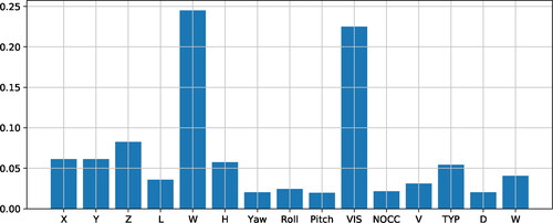
As shown in Table 4, the ML algorithms use a total of 15 input parameters to decide whether an object is detected or undetected by the radar. To evaluate the importance of each individual input parameter for the applied ML algorithms, the concept of feature importance (Breiman, 2001) was applied. The feature importance represents a weight assigned to the respective feature. The value represents the total reduction of the criterion brought by that feature. Hence, the higher the value, the more important the feature. The feature importance calculation methods for the linear SVC model, the Random Forest model, and the Gradient Boosting model are implemented in the used python libraries. For the linear SVC model, the attribute coef_ from the class sklearn.svm.SVC is used. For the Random Forest model, the attribute feature_importances_ from the class sklearn.ensemble.RandomForest Classifier is used. And for the Gradient Boosting model, the property feature_importances_ from the python class xgboost.XGBClassifier is used. Figures 12–14 depict the feature importance values of all 15 input parameters for the linear SVC model, the Random Forest model, and the Gradient Boosting model respectively. The most important input parameter for the linear SVC model is the object class TYP with a value of 0.8. All remaining input parameters have a feature importance value well below. The most important features for the Random Forest model are the vertical object position Z, the object width W, and the visibility VIS. The Random Forest model’s feature importance values are more equally distributed compared to the feature importance values of the linear SVC model and the Gradient Boosting model. Only daytime DT, weather condition W, and the number of occluders NOCC have feature importance values less than 0.02. The most important features for the Gradient Boosting model are the object width W and the visibility VIS with values of around 0.20 − 0.25. The feature importance values of the other parameters are well below.

Figure 12. Feature importance of all 15 input parameters for the linear SVC model.

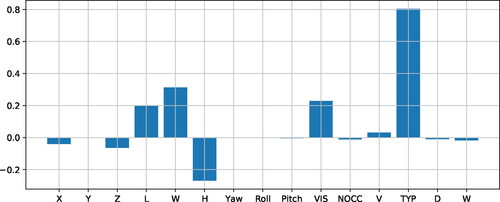
Figure 13. Feature importance of all 15 input parameters for the Random Forest model.

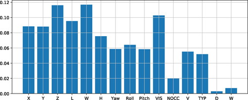
Figure 14. Feature importance of all 15 input parameters for the Gradient Boosting model.

13. Discussion and conclusion

This article presents a thorough analysis of the nuScenes radar data and four radar models on object level with different complexity levels and parametrisation requirements. The considered radar type (Continental ARS-408-21) is a very common, state-of-the-art automotive radar and the aspects addressed in this article may also be applicable to other automotive radar types.

The detection threshold of the radar is found to be around 0 dBsm in most parts of the FOV, proposing no limitation to detect both vehicles and pedestrians. Only at distances between 40 − 70 m and at high incidence angles ($\theta =25-{40}^{°}$), the threshold values are distinct higher (5 − 10 dBsm), lowering the chance to detect smaller targets, such as pedestrians and bikes. Only 11% of all radar detections could be assigned to a labeled object. The remaining 89% are considered clutter or false positive detections, which can arise from unlabeled infrastructure (buildings, bridges, tunnels, etc.) and effects such as multi-path propagation and interferences. No radar cluster point with less than −10 dBsm, or more than 60 dBsm was found in the data. These values represent most likely the detection boundaries of the considered radar type.

The radar measurements were linked to the labeled objects and a quantitative analysis of the reflection properties of different object classes is given. Note that the provided RCS values include the weighting by the signal processing inside the Continental ARS-408-21. The yaw angle ψ of the object relative to the radar seems to have only minor influence on the measured RCS value. Even though the minimum and maximum measured RCS values show a negative and positive peak at $0^{°}$ and ${90}^{°},$ this is most likely caused by a much higher number of observed objects in these angles.

Radar detection probabilities P_D were evaluated depending on range, viewing angle, object class, daytime and weather conditions, and additionally calculated object parameters, such as number of occluders NOCC, relative visible area VIS, and object velocity. The detection probability P_D is highest close to the sensor and at small viewing angles, which is expected according to the antenna pattern of the radar. The main lobe of the radiation pattern is clearly visible in the spatial P_D distribution. The side lobes are not visible and may have a negligible effect. Big vehicles are the only object class with a $P_D>50 \%.$ In particular, pedestrians have a very low detection probability (around 8%). Hence, this type of radar is probably not a good choice for the detection of vulnerable road users, even though the detection probability of pedestrians might increase in the close proximity to the sensor and when considering multiple radar scans for object detection. Daytime and weather conditions seem to have only a minor influence on the detection probability, which shows that this type of radar is well suited for operation under adverse weather conditions. As shown by Hasirlioglu and Riener (2017), fog and light rain have only a very small impact on radar measurements, but the attenuation during heavy rain might still have a considerable impact on long-distance measurements and can reduce the maximum detection range. Having no other object in the line-of-sight between radar and target (NOCC = 0), is clearly favorable for the detection probability, but even in cases, where several objects occlude the target, the detection probability is still around 20%. Completely occluded objects ($\mathit{VIS}=0 \%$) are improbable to be detected by the radar, but occlusion values up to 80% seem to have only a minor influence. The radar is clearly able to detect objects, even if several other objects partly or completely cover the direct line-of-sight. This is most likely caused by fact that radar waves can travel through certain objects, very close along the object edges, and via multi-path propagation on the road or infrastructure elements indirectly to the target. Objects that move with $>2.5m/s$ relative to the environment have a distinct higher detection probability than objects that are slower or standing. This is probably caused by the fact that the radar is using the Doppler shift in the return signal to separate moving targets from the surrounding environment. A moving target might therefore have a higher chance to get a radar cluster point assigned.

Four radar models on object level with two different levels of complexity and parametrisation requirements were built and analyzed.

The first model is a simple RCS-based radar model that uses radar detection thresholds and object RCS values and requires for parametrisation only a radar specification sheet. Inside the FOV, almost all objects were considered detected, apart from smaller objects at high viewing angles θ. The RCS-based model represents an ideal sensor model similar to most sensor models in currently available virtual test environments. The accuracy of this model type was found to be around 50%, illustrating the importance of taking additional radar, object and environmental parameters into account.

Three radar models based on supervised machine learning (ML) algorithms were built, each using a total of 15 object and environmental parameters as input. These models require for parametrisation the collection of a representative dataset, including ground-truth information, which proposes a considerable effort. The ML-based models can achieve an accuracy of more than 85% and are therefore well suited for virtual testing of ADAS/AD functions. The remaining 15% inaccuracy might be explained by a combination of missing input factors and uncertainties due to statistical variations. Other potentially influencing factors are static objects that are not annotated in the nuScenes dataset and therefore not taken into account by the ML-based models, e.g., tunnels, bridges, houses, and other metal structures. Additional uncertainties arise due to, e.g., the statistical variations of radar properties within a single object class. Based on the conducted feature importance analysis of the ML algorithms, the following object parameters can be considered as important for radar modeling: object type, object position, object size, and object visibility VIS. The following object parameters can be considered least important and might, therefore, be neglected: daytime, weather conditions, and number of occluders OCC.

A drawback of the presented models is their lack to simulate additional false positive object detections that are not in the ground-truth object list, i.e. the models only reduce the amount of existing objects, but are not able to create new non-existing objects. This limitation is related to the fact that the radar data in the nuScenes dataset includes only radar clusters but no object lists. In order to assess how many and which radar clusters that could not be assigned to an object, cause a false positive object detection, one would need to apply an object detection algorithm. Unfortunately, radar manufacturers are very protective about their object detection algorithms and we were therefore not able to perform this assessment.

14. Outlook

The following two areas for further research were identified:

• The presented processing chain for radar data shall be adapted and applied in a similar manner on the nuScenes lidar data. This shall lead to a better understanding of the relevant object and environmental parameters for automotive lidar applications, the development of lidar models, and a comparison lidar versus radar based on a large amount of labeled scenarios.

• The radar cluster data in the nuScenes dataset allow to build a ML-based radar model on raw data level. This model shall be developed and evaluated. The processing chain of the planned ML-based radar model on raw data level is similar to the processing chain shown in Figure 11. However, instead of a detection decision for each object, the ML-algorithm shall provide a number of cluster points NC including corresponding RCS values for each object inside the radar’s FOV. The radar cluster points can then serve as input for an object recognition function, which eventually provides an object list for the ADAS/AD function under test.

Abbreviations
AD	=	automated driving
ADAS	=	advanced driver assistance system
D	=	detected objects
DT	=	daytime
FOV	=	field of view
ML	=	machine learning
NC	=	number of radar clusters
NOCC	=	number of occluders
PD	=	detection probability
SVC	=	support vector classifier
PDF	=	probability density function
RCS	=	radar cross section
U	=	undetected objects
VIS	=	visibility
W	=	weather conditions

Acknowledgments

The publication was written at Virtual Vehicle Research GmbH in Graz, Austria. The authors would like to acknowledge the financial support within the COMET K2 Competence Centers for Excellent Technologies from the Austrian Federal Ministry for Climate Action (BMK), the Austrian Federal Ministry for Digital and Economic Affairs (BMDW), the Province of Styria (Dept. 12) and the Styrian Business Promotion Agency (SFG). The Austrian Research Promotion Agency (FFG) has been authorised for the programme management. They would furthermore like to express their thanks to their supporting industrial and scientific project partners, namely AVL List GmbH, Infineon Technologies Austria AG, Ing. h. c. F. Porsche AG, Volkswagen AG, ZF Friedrichshafen AG and Technical University Graz. A special thanks to the two anonymous reviewers for valuable input that improved our paper.

Disclosure statement

No potential conflict of interest was reported by the author(s).

Table

		linear SVC model
		undetected	detected	Total
radar measurements	undetected	24554	19609	44163
	detected	7334	37082	44416
	Total	31888	56691	88579

$\to \mathit{Accuracy}=69.58 \%,\mathit{Precision}=65.41 \%,\mathit{Recall}=83.49 \%.$

Table

		Random Forest model
		undetected	detected	Total
radar measurements	undetected	36145	8018	44163
	detected	6726	37690	44416
	Total	42871	45708	88579

$\to \mathit{Accuracy}=83.35 \%,\mathit{Precision}=82.46 \%,\mathit{Recall}=84.86 \%.$

Table

		Gradient Boosting model
		undetected	detected	Total
radar measurements	undetected	37511	6652	44163
	detected	6191	38225	44416
	Total	43702	44877	88579

$\to \mathit{Accuracy}=85.50 \%,\mathit{Precision}=85.18 \%,\mathit{Recall}=86.06 \%.$

Additional information

Funding

This research received financial support within the COMET K2 Competence Centers for Excellent Technologies from the Austrian Federal Ministry for Climate Action (BMK), the Austrian Federal Ministry for Digital and Economic Affairs (BMDW), the Province of Styria (Dept. 12) and the Styrian Business Promotion Agency (SFG).

References

- Anderson, J. M., Kalra, N., Stanley, K. D., Sorensen, P., Constantine, S., Oluwatobi, A. (2016). ‘Autonomous Vehicle Technology: A Guide for Policymakers’ RAND Corporation, RR-443-2-RC, Santa Monica, Calif., Retrieved January 23, 2020, from http://www.rand.org/pubs/research_reports/RR443-2.html
- Arage, A., Steffens, W. M., Kuehnle, G., & Jakoby, R. (2006). ‘Effects of Water and Ice Layer on Automotive Radar’ in Proc. German Microw. Conf,
- Bernsteiner, S., Magosi, Z., Lindvai-Soos, D., Eichberger, A., Lindvai-Soos, D., & Eichberger, A. (2015). Radarsensormodell fuer den virtuellen Entwicklungsprozess. ATZelektronik, 10(2), 72–79. https://doi.org/10.1007/s35658-015-0508-y
- Breiman, L. (2001). Random Forests. Machine Learning 45, 5–32. https://doi.org/10.1023/A:1010933404324
- Buehren, M., & Bin, Y. (2006a). Automotive radar target list simulation based on reflection center representation of objects. In Proc. Intern. Workshop on Intelligent Transportation (WIT), Germany. pp. 161–166.
- Buehren, M., & Bin, Y. (2006b). Simulation of automotive radar target lists using a novel approach of object representation. (pp. 314–319). IEEE Intelligent Vehicles Symposium (IV).
- Buehren, M., & Bin, Y. (2007a). A Global Motion Model for Target Tracking in Automotive Applications. In Proceedings of IEEE International Conference on Acoustics, Speech and Signal Processing (ICASSP), 2, II-313–II-316. https://doi.org/10.1109/ICASSP.2007.366235
- Buehren, M., & Bin, Y. (2007b). Extension of Automotive Radar Target List Simulation to consider further Physical Aspects. In Proceedings of 7th International Conference on Intelligent Transport Systems (ITS) Telecommunications, 1–6, June 2007. https://doi.org/10.1109/ITST.2007.4295847
- Buehren, M., & Bin, Y. (2007c). Initialization procedure for radar target tracking without object movement constraints. In Proceedings of 7th International Conference on Intelligent Transport Systems (ITS) Telecommunications, 112–117, June 2007. https://doi.org/10.1109/ITST.2007.4295845
- Buehren, M., & Bin, Y. (2007d). Simulation of Automotive Radar Target Lists considering Clutter and Limited Resolution. In Proceedings of International Radar Symposium, pp. 195–200, September 2007.
- Caesar, H., Bankiti, V., Lang, A. H., Vora, S., Liong, V. E., Xu, Q., Krishnan, A., Pan, Y., Baldan, G., & Beijbom, O. (2019). nuScenes: A multimodal dataset for autonomous driving. CoRR, volume abs/1903.11027, arXiv:1903.11027v1 [cs.LG].
- Cao, P., Wachenfeld, W., & Winner, H. (2015). Perception sensor modeling for virtual validation of automated driving. IT - Information Technology, 57(4), 243–251. https://doi.org/10.1515/itit-2015-0006
- Cao, P. (2017). Modeling active perception sensors for real-time virtual validation of automated driving systems [PhD thesis]. Technische Universität Darmstadt
- Continental. (2016). Technical Documentation ARS 404-21 (Entry) and ARS 408-21 (Premium). Continental Engineering Services GmbH Version 1.0, 14 October
- Continental. (2017). ARS 408-21 Premium Long Range Radar Sensor 77 GHz. Continental Engineering Services GmbH, ARS 408-21 datasheet.
- Cordts, M., Omran, M., Ramos, S., Rehfeld, T., Enzweiler, M., Benenson, R., Franke, U., Roth, S., & Schiele, B. (2016). The cityscapes dataset for semantic urban scene understanding. In Proceedings of the IEEE Conference on Computer Vision and Pattern Recognition (CVPR).
- Cortes, C., & Vapnik, V. (1995). Support-vector networks. Machine Learning, 20(3), 273–297. https://doi.org/10.1007/BF00994018
- Danielsson, L. (2010). Tracking and radar sensor modelling for automotive safety systems [PhD thesis]. Chalmers University of Technology.
- Dosovitskiy, A., Ros, G., Codevilla, F., Lopez, A., Koltun, V. (2017). CARLA: An Open Urban Driving Simulator. In Proceedings of the 1st Annual Conference on Robot Learning, 1–16.
- Echard, J. D. (1991). ‘Estimation of radar detection and false alarm probability’. IEEE Transactions on Aerospace and Electronic Systems, 27(2), 255–260. https://doi.org/10.1109/7.78300
- Eltayeb, M. E., Al-Naffouri, T. Y., & Robert, W. (2018). Heath compressive sensing for millimeter wave antenna array diagnosis. IEEE Transactions on Communications, 66(6), 2708–2721. in http://ieeexplore.ieee.org/stamp/stamp.jsp?tp=&arnumber=8248776&isnumber=8385566 https://doi.org/10.1109/TCOMM.2018.2790403
- Fagnant, D. J., & Kockelman, K. (2015). Preparing a nation for autonomous vehicles: opportunities, barriers and policy recommendations. Transportation Research Part A: Policy and Practice, 77, 167–181. https://doi.org/10.1016/j.tra.2015.04.003. http://www.sciencedirect.com/science/article/pii/S0965856415000804
- Friedman, J. H. (2001). Greedy function approximation: A gradient boosting machine. The Annals of Statistics, 29(5), 1189–1232. https://doi.org/10.1214/aos/1013203451
- Friedman, J., Hastie, T., & Tibshirani, R. (2000). Additive logistic regression: a statistical view of boosting (With discussion and a rejoinder by the authors)’. The Annals of Statistics, 28(2), 337–407. https://doi.org/10.1214/aos/1016218223
- Geiger, A., Lenz, P., & Urtasun, R. (2012). Are we ready for autonomous driving? The KITTI vision benchmark suite. In Proc. IEEE Conf. Comput. Vis. Pattern Recognit, 3354–3361.
- Geiger, A., Lenz, P., Stiller, C., & Urtasun, R. (2013). Vision meets robotics: The KITTI Dataset. The International Journal of Robotics Research, 32(11), 1231–1237. https://doi.org/10.1177/0278364913491297
- Hakuli, S., & Krug, M. (2015). ‘Virtuelle Integration’ Kapitel 8 in Handbuch Fahrerassistenzsysteme - 2015. In H. Winner (Ed.), Grundlagen, Komponenten und Systeme fuer aktive Sicherheit und Komfort. Springer Verlag.
- Hammarstrand, L., Lundgren, M., & Svensson, L. (2012a). Adaptive radar sensor model for tracking structured extended objects. IEEE Transactions on Aerospace and Electronic Systems, 48, 1975–1995. https://doi.org/10.1109/TAES.2012.6237574,July 2012.
- Hammarstrand, L., Svensson, L., Sandblom, F., & Sorstedt, J. (2012b). Extended object tracking using a radar resolution model. IEEE Transactions on Aerospace and Electronic Systems, 48, 2371–2386. https://doi.org/10.1109/TAES.2012.6237597
- Hanke, T., Hirsenkorn, N., Dehlink, B., Rauch, A., Rasshofer, R., & Biebl, E. (2015). Generic Architecture for Simulation of ADAS Sensors. 2015 In Proceedings International Radar Symposium, Dresden.
- Hanke, T., Hirsenkorn, N., van-Driesten, C., Garcia-Ramos, P., Schiementz, M., Schneider, S., & Biebl, E. (2017). Open Simulation Interface - A generic interface for the environment perception of automated driving functions in virtual scenarios. Research Report. https://www.hot.ei.tum.deforschungautomotive-veroeffentlichungen.
- Hasch, J. (2015). Driving Towards 2020: Automotive Radar Technology Trends. In IEEE MTT-S International Conference on Microwaves for Intelligent Mobility, 978-1-4799-7215-9/15, 1–4.
- Hasirlioglu, S., & Riener, A. (2017). Introduction to rain and fog attenuation on automotive surround sensors. In 2017 IEEE 20th International Conference on Intelligent Transportation Systems (ITSC), Yokohama, 1–7. https://doi.org/10.1109/ITSC.2017.8317823,2017.
- Hasirlioglu, S., Kamann, A., Doric, I., & Thomas, B. (2016). Test Methodology for Rain Influence on Automotive Surround Sensors. In 2016 IEEE 19th International Conference on Intelligent Transportation Systems (ITSC) Windsor Oceanico Hotel, Rio de Janeiro, Brazil, November 1-4.
- Hassen, A. A. (2007). Indicators for the signal degradation and optimization of automotive radar sensors under adverse weather conditions [Dissertation]. TU Darmstadt. http://elib.tu-darmstadt.de/diss/000765,
- Hirsenkorn, N., Hanke, T., Rauch, A., Dehlink, B., Rasshofer, R., & Biebl, E. (2015). A non-parametric approach for modeling sensor behavior. 16th International Radar Symposium, pp. 131–136.
- Hirsenkorn, N., Subkowski, P., Hanke, T., Schaermann, A., Rauch, A., Rasshofer, R., & Biebl, E. (2017). A ray launching approach for modeling an FMCW radar system [Paper presentation]. The 18th International Radar Symposium IRS 2017, Prague, Czech Republic, June 28-30, pp. 1–10. https://doi.org/10.23919/IRS.2017.8008120
- Huang, X., Cheng, X., Geng, Q., Cao, B., Zhou, D., Wang, P., Lin, Y., Yang, R. (2018). The ApolloScape Dataset for Autonomous Driving. IEEE Conference on Computer Vision and Pattern Recognition (CVPR) Workshops, 954–960.
- Huang, X., Wang, P., Cheng, X., Zhou, D., Geng, Q., & Yang, R. (2019). The ApolloScape open dataset for autonomous driving and its application. IEEE Transactions on Pattern Analysis and Machine Intelligence, 42(10), 2702–2719. arXiv:1803.06184v4. https://doi.org/10.1109/TPAMI.2019.2926463
- IPG. (2019). Automotive GmbH ‘CarMaker: Virtual testing of automobiles and light-duty vehicles’. Retrieved October 2, 2019, from https://ipg-automotive.com/products-services/simulation-software/carmaker/.
- Kalra, N., & Paddock, S. M. (2016). Driving to safety: How many miles of driving would it take to demonstrate autonomous vehicle reliability? Transportation Research Part A: Policy and Practice, 94, 182–193. https://doi.org/10.1016/j.tra.2016.09.010. http://www.sciencedirect.com/science/article/pii/S0965856416302129
- Kang, Y., Yin, H., & Berger, C. (2019). Test your self-driving algorithm: an overview of publicly available driving datasets and virtual testing environments. IEEE Transactions on Intelligent Vehicles, 4(2), 171–185. https://doi.org/10.1109/TIV.2018.2886678
- Liebske, R. (2019). ‘Short Description ARS 404-21 (Entry) + ARS 408-21 (Premium) Long Range Radar Sensor 77 GHz - Technical Data’ Continental, Version 1.11en, document no. 2017_07_09-10,
- Maier, F. M., Makkapati, V. P., & Horn, M. (2018a). Adapting phong into a simulation for stimulation of automotive radar sensors. IEEE International Conference on Microwaves for Intelligent Mobility. https://doi.org/10.1109/ICMIM.2018.8443493
- Maier, F. M., Makkapati, V. P., & Martin, H. (2018b). Environment perception simulation for radar stimulation in automated driving function testing. Elektrotechnik & Informationstechnik, 135, 1–7. 135/4-5: 309–315. https://doi.org/10.1007/s00502-018-0624-5,
- Marti, E., Perez, J., de Miguel, M. A., & Garcia, F. (2019). A review of sensor technologies for perception in automated driving. IEEE Intelligent Transportation Systems Magazine, pp. 94–108, Winter 2019. https://doi.org/10.1109/MITS.2019.2907630
- Mesow, L. (2006). Multisensorielle Datensimulation im Fahrzeugumfeld für die Bewertung von Sensorfusionsalgorithmen [PhD thesis], Technische Universität Chemnitz.
- Meyer, M., & Kuschk, G. (2019). Automotive Radar Dataset for Deep Learning Based 3D Object Detection. In Proceedings of the 16th European Radar Conference, Paris, France, 2–4 October 2019, pp. 129–132.
- Muckenhuber, S., Holzer, H., Rübsam, J., & Stettinger, G. (2019). Object-Based Sensor Model for Virtual Testing of ADAS/AD Functions. IEEE ICCVE (International Conference on Connected Vehicles and Expo), Graz, 4-8 November 2019.
- Patole, S. M., Torlak, M., Wang, D., & Ali, M. (2017). Automotive radars: A review of signal processing techniques. IEEE Signal Processing Magazine, 34(2), 22–35. https://doi.org/10.1109/MSP.2016.2628914, http://ieeexplore.ieee.org/stamp/stamp.jsp?tp=&arnumber=7870764&isnumber=7870726
- Ramasubramanian, K., & Ramaiah, K. (2018). Moving from Legacy 24 GHz to State-of-the-Art 77-GHz Radar. ATZelektronik Worldwide, 13, 46–49. https://doi.org/10.1007/s38314-018-0029-6
- SAE. (2018). SAE International ‘Ground Vehicle Standard J3016_201806’, Retrieved January 20, 2020, from https:saemobilus.sae.orgcontentj3016_201806
- Schlager, B., Muckenhuber, S., Schmidt, S., Holzer, H., Rott, R., Maier, F. M., Saad, K., Kirchengast, M., Stettinger, G., Watzenig, D., & Ruebsam, J. (2020). State-of- the-art sensor models for virtual testing of advanced driver assistance systems/autonomous driving functions. SAE International Journal of Connected and Automated Vehicles, 3(3), 233–261. https://doi.org/10.4271/12-03-03-0018
- Schuler, K. (2007). Intelligente Antennensysteme für Kraftfahrzeug-Nahbereichs-Radar-Sensorik. PhD thesis Universität Karlsruhe (TH).
- Schuler, K., Becker, D., & Wiesbeck, W. (2008). Extraction of virtual scattering centers of vehicles by ray-tracing simulations. IEEE Transactions on Antennas and Propagation, 56, 11.
- Shah, S., Dey, D., Lovett, C., Kapoor, A. (2017). AirSim: High-Fidelity Visual and Physical Simulation for Autonomous Vehicles’ Field and Service Robotics. arXiv:1705.05065, https://arxiv.org/abs/1705.05065,
- Stolz, M., & Nestlinger, G. (2018). Fast Generic Sensor Models for Testing Highly Automated Vehicles in Simulation. Elektrotechnik Und Informationstechnik, 135(4-5), 365–369. https://doi.org/10.1007/s00502-018-0629-0
- Sun, P., Kretzschmar, H., Dotiwalla, X., Chouard, A., Patnaik, V., Tsui, P., Guo, J., Zhou, Y., Chai, Y., Caine, B., Vasudevan, V., Han, W., Ngiam, J., Zhao, H., Timofeev, A., Ettinger, S., Krivokon, M., Gao, A., Joshi, A. … Anguelov, D. (2019). Scalability in Perception for Autonomous Driving: Waymo Open Dataset. arXiv:1912.04838v5 [cs.CV] 18.
- VIRES. (2019). VIRES Simulationstechnologie GmbH. VTD - VIRES Virtual Test Drive. Retrieved October 2, 2019. https://vires.com/vtd-vires-virtual-test-drive/
- Watzenig, D., & Horn, M. (Eds.). (2016). Automated driving: safer and more efficient future driving. Springer. https://doi.org/10.1007/978-3-319-31895-0
- Wheeler, T. A., Holder, M., Winner, H., Kochenderfer, M. J. (2017). Deep Stochastic Radar Models, In IEEE Intelligent Vehicles Symposium.
- World Health Organisation (WHO). (2018). Global status report on road safety 2018. ISBN 978-92-4-156568-4, Retrieved January 20, 2020, from https://apps.who.int/iris/bitstream/handle/10665/276462/9789241565684-eng.pdf.
- Xu, H., Gao, Y., Yu, F., & Darrell, T. (2017). End-to-end learning of driving models from large-scale video datasets. In Proceedings of IEEE Conference on Computer Vision Pattern Recognition, 3530–3538.
- Yu, F., Xian, W., Chen, Y., Liu, F., Liao, M., Madhavan, V., & Darrell, T. (2018). BDD100K: A diverse driving video database with scalable annotation tooling. arXiv:1805.04687.