Research on coordinated control of vehicle’s speed in new mixed traffic flow

Abstract

The emerging intelligent connected technology provides conditions for obtaining the trajectory of vehicles. To reduce the adverse effects of stop-and-go vehicles in the bottleneck section of expressways, a strategy of coordinated speed control based on trajectory is proposed in a single-lane. Firstly, the trajectories of the connected and autonomous vehicles (CAV) in the downstream vehicle cluster are offset and modified to predict the trajectory of the last human vehicle (HV) based on the information collected by the road side traffic sensors and combined with the speed of traffic wave and the driver’s reaction time. Then, according to the predicted trajectory, the velocity distribution of the first CAV in the vehicle cluster upstream at different time points is planned to restrain the propagation of velocity oscillation, the CAV can gradually merge into the downstream traffic flow at a more reasonable and smooth speed. Finally, the influence of different factors on the suppression of speed oscillation are analyzed by numerical simulation. The results show that: within the numerical simulation range of the designed CAV permeability of 0%∼25% and the starting position of the bottleneck is 575 m∼975 m, the higher the permeability, the farther the starting position of the bottleneck and the smoother the speed curve selected by CAV, the stronger the suppression of speed oscillations, and at the same time it proves that the strategy of coordinated speed control can effectively reduce the fluctuation of traffic flow, improve driver comfort and overall efficiency of vehicle queue.

Keywords:

• Mixed traffic flow
• numerical simulation
• speed coordination
• traffic oscillation
• trajectory prediction

1. Introduction

Traffic oscillation is a common phenomenon in traffic flow. It is the macroscopic performance of vehicles that accelerate and decelerate under the drive or stimulation of external environmental factors to make the traffic flow stop and go. Traffic oscillation may cause a significant decrease in traffic efficiency, increase the risk of vehicle collisions, and affect driving comfort. In the past two decades, scholars have conducted further research on the formation and propagation mechanism of traffic oscillations. Qin et al. (2021) observed the spontaneous formation, propagation and development of oscillations within the velocity and evaluated reductions of emissions and fuel consumption under traffic oscillations. Vehicle lane changing activities may lead to the formation of traffic oscillations (Ahn & Cassidy, 2007; Laval & Daganzo, 2006) and the large individuals, e.g., slow-moving trucks, may also cause traffic oscillations by Laval (2007). In addition, changes in ramps and road geometry may also lead to the formation of traffic oscillations in Li et al. (2012). Regarding the spread of traffic oscillations, Laval and Leclercq (2010) believed that timid and aggressive driving behavior (heterogeneity of human drivers) is the cause of the spread of traffic oscillations. Zheng et al. (2011) found that the propagated speed of oscillation, oscillation’s duration and amplitude are similar and all observed phenomena initially exhibited the precursor phase, which is the localization of slow motion and movement, after which the oscillations propagate upstream in the queue. A common method to suppress traffic oscillation is speed coordination, which reduce the time and space changes of vehicle speed by applying certain control methods. One work to be done before speed coordination is to judge the downstream traffic status. A real-time traffic state evaluation method based on the advantages of the urban cooperative vehicle infrastructure system (CVIS) was proposed by Wang et al. (2019), which could improve the real-time and objectivity of the traffic state evaluation results, and it provided a basis for real-time traffic guidance. In tradition, the methods of variable speed limit (VSL) and speed recommended value can be applied to speed coordination to minimize vehicle speed changes. Wang et al. (2020) have established a joint control model which optimizing the speeds of the connected vehicles and coordinating signals along an arterial simultaneously. Han et al. (2017) and Soriguera et al. (2017) also studied the guidance of speed through theoretical analysis method and empirical verification method respectively. On urban roads, Kattan et al. (2015) presented the results of an evaluation of a candidate VSL system that takes the space mean speeds (SMSs) from probe vehicles as its main input. The presented algorithm extends the capability of a model predictive control (MPC) VSL model. Pang and An (2019) proposed the speed guidance adaptive control method of urban expressway according to the upstream vehicle destination of the main line, so as to significantly improve the regional flow.

Although these studies provide valuable insights on speed coordination techniques, most existing studies can only suggest or force human drivers to adjust their speed. The unpredictability of human behavior may make these methods fail, and it may not be possible to obtain smooth speeds by using traditional speed coordination control strategies. And although the research on the probe vehicle data and video extracted traffic flow data have been studied for many years, most of them were mainly focused on mining historical traffic flow data, limited to the parameters such as section flow, speed and occupancy and these parameters were applied to scenarios such as travel time estimation, traffic signal control and traffic guidance. With the rapid development of intelligent connected technologies, the information between the participants in the transportation system becomes more real-time and reliable. CAVs can share their running trajectories in real time, which can help drivers predict the traffic environment information in advance. Many studies have begun to use CAV technology to develop and improve speed coordination strategies (Ghiasi et al., 2017; Guo et al., 2019; Wang et al., 2016; Zhao et al., 2018). Motamedidehkordi et al. (2016) presented the inter-vehicles communication in a shock wave traffic flow scenario with the discussion of performance indicators. They found out that, with an increasing penetration rate of V2V equipped vehicles, which can receive the traffic jam ahead warning, the congestion propagates on the freeway with slower speed and the congestion area becomes smaller. Most of these studies are still focused on urban roads, and using the color information of signal light to control a single CAV. In addition, most of the existing researches consider the fully automated driving scenario, but there will be a state of mixed driving of CAV and HV for a long period of time in the future.

This paper proposes a strategy about speed coordination based on trajectory under the background of this new mixed traffic flow. It should be noted that this study is only applicable to expressways without intersections and signal control. There are two main contributions in this study.

• We use real-time data of traffic sensors and real-time information provided by the downstream CAV to predict the trajectory of the HV in the future.

• We try our best to make the planned upstream CAV’s speed smoother to suppress traffic shock and spread in order to improve the stability of expressway traffic flow and the comfort of drivers.

The rest of this paper is organized as follows. Section 2 summaries the steps of control Strategy. Section 3 illustrates the scene building. Section 4 proposed the trajectory prediction of HV. Section 5 proposed the speed planning of CAV. Section 6 performs numerical simulation analysis. Section 7 shows the results discussion and Section 8 concludes.

2. Steps of control strategy

This paper proposes a real-time control strategy by using CAV to coordinate speed. The information provided by CAV and traffic sensors is used to detect the decrease in the speed of downstream vehicles or oscillations and predict their upstream propagation. Then, we control the speed of the CAV upstream of the bottleneck so that the propagation of speed oscillations is suppressed and subsequent vehicles run at a smooth speed. Ideally, the speed of CAV should enable the upstream traffic flow to proceed smoothly and steadily in the upstream position of the bottleneck until the queue at the bottleneck dissipates and the speed of the traffic flow recovers. The proposed strategy consists of three main steps.

Step1: Scene building. Set the scenario to which the strategy is applicable, i.e., the single-lane section of the expressway. We assume that the traffic flow only contains HVs and CAVs. CAVs are equipped with necessary sensors, so they can record and share their real-time trajectories. We suppose that there are multiple vehicle clusters driving on the highway. Vehicle cluster refers to a stream of vehicles moving in a certain direction on the road with close interaction. It is the result of a self-organized behavior of vehicles to achieve the balance between driving safety and efficiency. Every vehicle cluster can contain multiple CAVs and HVs. More realistically, CAVs are randomly distributed in the traffic flow. But in this study, we assume that each vehicle cluster contains at least one CAV, and the pilot vehicle of cluster is CAV.

In the actual vehicle cluster, there will also be the case that HV is the pilot vehicle, and the subsequent CAV may be restricted by the HV in front when executing its own planned speed. In this case, CAV will exit the execution planning mode and give priority to the normal car-following with the preceding vehicle to ensure safety. The continuous CAVs in the traffic flow will drive according to their respective planning speed according to the designed method. At the same time, we deploy traffic sensors in different locations to collect the information of traffic volume $q_s\left(t\right)$ and density ${\rho }_s\left(t\right).$

Step 2: Predicting the trajectory of HV. Since the fluctuation of traffic flow will attenuate to a certain extent along the upstream direction with time, we use the CAVs of the preceding vehicle cluster to predict the trajectory of the last vehicle in this cluster, and we use the information of traffic sensors by the road to correct the predicted result. It provides support for the CAV speed planning of upstream vehicle clusters. It should be noted that we only need to predict the trajectory where the last HV in the front cluster, and use $r^{\mathrm{\text{'}}}(t^{\mathrm{\text{'}}}),\forall t^{\mathrm{\text{'}}}\ge t$ to express.

Step 3: Planning the speed of CAV. In this step, we design the subsequent CAV’s speed according to the predicted HV trajectory, so as to reduce the backward propagation of traffic oscillation and fluctuation caused by the excessive speed change rate of vehicles. Because of the single lane road section, the planning speed proposed in this paper is only a reasonable speed allocation in one-dimensional space, and the goal is to make the vehicle cluster guided by the upstream CAV converge into the downstream traffic flow at the speed of the HV ahead.

3. Scene building

We assume that a single lane section of an expressway contains two groups of vehicle clusters, denoted as$C_{1 }$ and $C_2.$ The number of traffic sensors denoted by $S$ are set on one side of the road, as shown in Figure 1.

Figure 1. Schematic diagram of scene building.

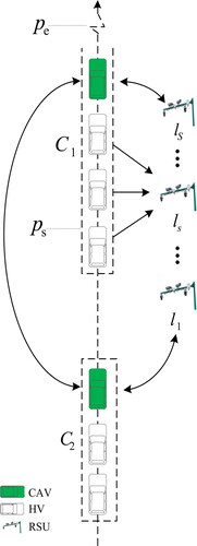
It is stipulated that HVs are a traditional vehicle without vehicle-vehicle and vehicle-road communication functions and CAVs integrate network connection and autonomous driving technology. We suppose that the detection range of the lidar sensor on CAV is 1 m∼200 m, the detection range of millimeter wave radar is 0.5 m∼250 m and their accuracy is ±0.1 m. The maximum relative speed obtained by millimeter wave radar is 240 km/h and the dedicate short-range communication (DSRC) delay for vehicle is less than 40 ms. The CAVs that guide each vehicle cluster can not only communicate with each other for information sharing, but also interact with road side sensors in real time. We suppose that at the current time $t_{1 }$ the last vehicle of the vehicle cluster${ C}_{1 }$ suddenly decelerates for a short time at the position $P_{\mathrm{S}}$ due to a certain stimulus of the preceding vehicle, and gradually returns to the normal speed at the downstream position $P_{\mathrm{e}}$ after the stimulus is removed. The duration of the whole process is recorded as $T,$ and we set the maximum speed limit of the highway as $v_{\mathrm{f}}.$

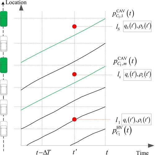
It should be noted that since the sensors information is updated at time point of decision making at a time interval of Δ$T,$ the downstream sensor will forward the measured $q_s(t\prime )$ and ${\rho }_s(t\prime )$ information to each individual CAV at intervals of ΔT. These data need to be represented in the middle of the time interval $\left[t-\Delta T,t\right],$ ($t^{\prime }=t-\Delta T/2$). Figure 2 is a schematic diagram of the information collected by the traffic sensor $l$ at time $t^{\prime }$ and the traffic status of each vehicle in the vehicle cluster $i$ at time$t.$ $p_i^{\mathrm{CAV}}(t),p_i^{\mathrm{HV}}(t)$ are respectively used to represent the positions of CAV and HV in vehicle cluster $i$ at time$t.$

Figure 2. Traffic information to be obtained.

It should be noted that when predicting the trajectory of the trailing vehicle of the cluster${ C}_{1 }$ after time $t,$ there are two types of following vehicle. The first case is that the following vehicle is CAV. In this case, the CAV can share the real-time speed and position information with the CAV of the vehicle cluster $C_{2 },$ which can accurately predict the last vehicle’s trajectory of the cluster${ C}_{1 }.$ The second case is that the following vehicle is HV, in this case, it is necessary to use the information collected by the road side sensors to measure the traffic volume and traffic density between the vehicle cluster ${ C}_{1 }$ and the vehicle cluster ${ C}_{2 }.$ And we use the transitivity of the CAV’s trajectory in the cluster ${ C}_{1 }$ to predict the last vehicle’s trajectory in the cluster ${ C}_{1 }.$ This article only studies the second, more general case.

4. Trajectory prediction of HV

In the second step of the strategy, information of CAVs and road side sensors will be used to predict the trajectory of the last vehicle in the downstream vehicle cluster. It is assumed that the evolution of the macroscopic traffic volume follows the triangular basic diagram. For the triangular basic diagram, a simplified version of the traffic wave theory proposed by Newell and the LWR model are used for prediction. Although the prediction is based on the simple Newell method, as long as their equilibrium state is consistent with the basic triangle diagram, they can be applied to the entire speed coordination process. The first is to predict the trajectory of the preceding HV based on CAV.

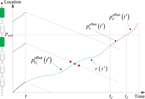
4.1. CAV trajectory offset

CAV provides conditions for predicting the trajectory of the vehicle ahead by sharing real-time information. Trajectory offset means that to obtain the trajectory of the HV behind, the trajectory of the CAV in front is shifted to the right for a reaction time ${\tau }_n,$ and to the down in space for a minimum safe distance $d_n$ as shown in Figure 3.

Figure 3. Schematic diagram of trajectory offset.

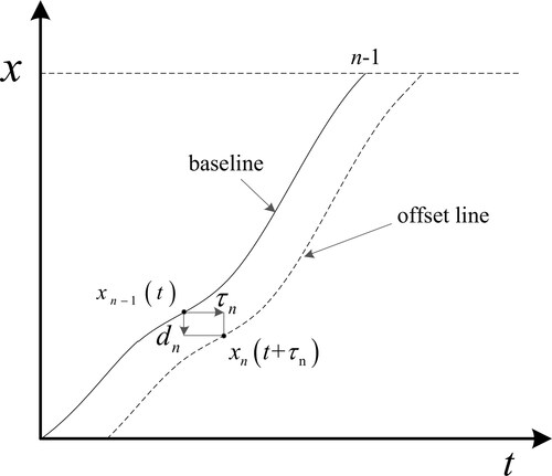
We assume that traffic state propagates upstream at wave speed $w,$ thus the right offset is $(m_{C_1}(t^{\mathrm{\text{'}}})-m_{C_1}^{\mathrm{CAV}}(t^{\mathrm{\text{'}}}))\frac{s_0}{w}$ and the downward offset is $(m_{C_1}(t^{\mathrm{\text{'}}})-m_{C_1}^{\mathrm{CAV}}(t^{\mathrm{\text{'}}}))s_0.$ Finally, we use an offset of the CAV trajectories and shift them along the backward wave in the time-space diagram. Let $r(t^{\mathrm{\text{'}}}),\forall t^{\mathrm{\text{'}}}\ge t$ denote the prediction function based on CAV. Let $p_{C_1}^{\text{offset}\mathrm{ }}$ denote the offset trajectory of each CAV in the vehicle cluster ${ C}_{1 }$after the current time $t.$ This set of trajectories is calculated using a simplified Newell model as follows: (1) $$p_{C_1}^{\text{offset}\mathrm{ }}\left(t^{\mathrm{\text{'}}}\right)=p_{C_1}^{\mathrm{CAV}}(t^{\mathrm{\text{'}}}-(m_{C_1}\left(t^{\mathrm{\text{'}}}\right)-m_{C_1}^{\mathrm{CAV}}\left(t^{\mathrm{\text{'}}}\right)\left)\frac{s_0}{w}\right)-\left(m_{C_1}\right(t^{\mathrm{\text{'}}})-m_{C_1}^{\mathrm{CAV}}(t^{\mathrm{\text{'}}}\left)\right)s_0$$(1) where $m_{C_1}(t^{\mathrm{\text{'}}})$ is the number of vehicles in the vehicle cluster ${ C}_{1 }$ at time$t^{\mathrm{\text{'}}};$ $s_0$ is the average car-following gap of all types of vehicles in the traffic bottleneck area; $m_{C_1}^{\mathrm{CAV}}\left(t^{\prime }\right)$ is the number of CAVs in the vehicle cluster ${ C}_{1 }$ at time $t^{\mathrm{\text{'}}},$ which can be obtained from the density and volume information collected by the road side sensors using the following formula: (2) $$m_{C_1}^{\mathrm{CAV}}\left(t^{\prime }\right)=m_s\left(t^{\prime }\right)+\left(p_{C_1}^{\mathit{CAV}}\left(t^{\prime }\right)-l_s\right){\rho }_s\left(t^{\prime }\right)$$(2) where $m_s\left(t^{\prime }\right)$ is the number of vehicles estimated by the sensor $s$ at the position of $l_s$ at time$t.$ It can be estimated in two ways: (1) Use the traffic volume information${ m}_s^{\mathrm{q}}\left(t^{\prime }\right)$ of the same traffic sensor, see equation (3)(3) $$m_s^{\mathrm{q}}\left(t^{\mathrm{\text{'}}}\right)=\frac{\mathrm{\Delta }T}{2}{q}_s\left(t^{\mathrm{\text{'}}}\right)$$(3) . (2) Use the density information $m_s^{\rho }(t^{\mathrm{\text{'}}})$ obtained by neighboring traffic sensors, see equation (4)(4) $$m_s^{\rho }\left(t^{\mathrm{\text{'}}}\right)=\frac{{\rho }_s\left({\mathrm{t}}^{\mathrm{\text{'}}}\right)+{\rho }_{s+1}\left(t^{\mathrm{\text{'}}}\right)}{2}(l_{s+1}-l_s)$$(4) . However, for all $s$=1, 2, …, $S,$ to improve the accuracy, better results can be obtained by the average of the estimated values of the two methods, that is formula (5). (3) $$m_s^{\mathrm{q}}\left(t^{\mathrm{\text{'}}}\right)=\frac{\mathrm{\Delta }T}{2}{q}_s\left(t^{\mathrm{\text{'}}}\right)$$(3) (4) $$m_s^{\rho }\left(t^{\mathrm{\text{'}}}\right)=\frac{{\rho }_s\left({\mathrm{t}}^{\mathrm{\text{'}}}\right)+{\rho }_{s+1}\left(t^{\mathrm{\text{'}}}\right)}{2}(l_{s+1}-l_s)$$(4) (5) $$m_s\left(t^{\mathrm{\text{'}}}\right)=\frac{m_s^{\mathrm{q}}\left(t\right)+m_s^{\rho }\left(t\right)}{2}$$(5)

Then, according to the number of CAVs of each group of vehicle clusters, it can be used to offset each CAV’s trajectory in the vehicle cluster${ C}_{1 }.$ The green dashed line in Figure 4 indicates the offset trajectory of the CAV in a vehicle cluster.

Figure 4. Correction of offset trajectory near${ p}_{\text{end}}.$

4.2. Offset correction

In this paper, triangle basic diagrams are used for both the upstream and downstream parts of the bottleneck. It should be noted that the difference of headway in space between CAV and HV and the difference of car-following gap in upstream and downstream traffic flow can cause some parts of the offset trajectory to jump as shown in Figure 4.

For the mixed traffic flow containing CAV, Qin et al. (2018) built the new LWR model for mixed traffic flow from the basic graph model under different CAV permeability. The general method is as follows:

Use ${ p}_{\mathrm{c}}{, p}_{\mathrm{h}}$ and ${ p}_{\mathrm{a}}$ to denote the proportions of CAV、 HV and AV in the mixed traffic flow, and use${ S}_{\mathrm{c}},$${ S}_{\mathrm{h}},$ and${ S}_{\mathrm{a}}$ to denote the space headway of CAV、HV and AV respectively in equilibrium. In the mixed traffic flow, the space headway varies according to the types of vehicles. It should be noted that at present, HVs has not been installed V2V communication equipment, and different types of vehicles in the mixed traffic flow are randomly distributed. When CAV follows HV, HV cannot transmit its own running status to the CAV through V2V communication, then this CAV obtains limited information of HV through its own on-board unit, that is, the CAV degenerates to AV, otherwise the CAV runs in CACC mode.

Therefore, the general expression of the "speed-space headway" relationship of the three types of vehicles in equilibrium is as follows: (6) $$\{\begin{array}{c}{S}_c=f_c\left(v_e\right)\\ S_h=f_h\left(v_e\right)\\ S_a=f_a\left(v_e\right)\end{array}$$(6) where $v_e$ is the velocity in equilibrium, m/s; $f_{\mathrm{c}}$、$f_{\mathrm{a}}$ and $f_{\mathrm{h}}$ are the "speed-to-space headway" function of CAV、AV and HV respectively in equilibrium.

According to the definition of traffic flow density, the density k of mixed traffic flow can be calculated as (7) $$k=\frac{1}{p_{\mathrm{c}}{S}_{\mathrm{c}}+p_{\mathrm{a}}{S}_{\mathrm{a}}+p_{\mathrm{h}}{S}_{\mathrm{h}}}$$(7)

Substituting equation (1)(1) $$p_{C_1}^{\text{offset}\mathrm{ }}\left(t^{\mathrm{\text{'}}}\right)=p_{C_1}^{\mathrm{CAV}}(t^{\mathrm{\text{'}}}-(m_{C_1}\left(t^{\mathrm{\text{'}}}\right)-m_{C_1}^{\mathrm{CAV}}\left(t^{\mathrm{\text{'}}}\right)\left)\frac{s_0}{w}\right)-\left(m_{C_1}\right(t^{\mathrm{\text{'}}})-m_{C_1}^{\mathrm{CAV}}(t^{\mathrm{\text{'}}}\left)\right)s_0$$(1) into equation (2)(2) $$m_{C_1}^{\mathrm{CAV}}\left(t^{\prime }\right)=m_s\left(t^{\prime }\right)+\left(p_{C_1}^{\mathit{CAV}}\left(t^{\prime }\right)-l_s\right){\rho }_s\left(t^{\prime }\right)$$(2) can get the basic graph relationship of "density-velocity" of mixed traffic flow: (8) $$k=\frac{1}{p_{\mathrm{c}}{f}_{\mathrm{c}}\left(v_e\right)+p_{\mathrm{a}}{f}_{\mathrm{h}}\left(v_e\right)+p_{\mathrm{h}}{f}_{\mathrm{a}}\left(v_e\right)}$$(8)

It can be seen from the above equation that the basic graph model of mixed traffic flow can be calculated by determining $f_{\mathrm{c}}\left(v_e\right),f_{\mathrm{h}}(v_e)$ and${ f}_{\mathrm{a}}(v_e)$_.

When p is used to represent the market rate of CAV in mixed traffic flow, the ratio of HV is 1-$p.$ if and only if CAV follows HV, the CAV will degenerate to AV, Then the probability of AV occurrence is the product of the proportion of CAV and HV, i.e.,$p (1-p),$ then the proportion of CAV with complete function in mixed traffic flow is $p-p(1-p)=p^2,$ i.e (9) $$\left\{\begin{array}{c}{p}_{\mathrm{c}}=p^2\\ p_{\mathrm{a}}=p(1-p)\\ p_{\mathrm{h}}=1-p\end{array}\mathrm{ }\text{and}\mathrm{ }\right\{\begin{array}{c}{p}_{\mathrm{c}}+p_{\mathrm{a}}+p_{\mathrm{h}}=1\\ p_{\mathrm{c}}+p_{\mathrm{a}}=p\\ p_{\mathrm{a}}\le p_{\mathrm{h}}\end{array}$$(9)

The above equations are the expression of mathematical expectation corresponding to the proportion of CAV、AV and HV in mixed traffic flow, and then the basic graph model of mixed traffic flow is analyzed and calculated.

The following model of CAV proposed by path laboratory is adopted as follows: (10) $$\{\begin{array}{c}{v}_n(t+\Delta t)=v_n\left(t\right)+k_p{e}_n\left(t\right)+k_d{\stackrel{.}{e}}_n\left(t\right)\\ e_n\left(t\right)=S_n\left(t\right)-l-h_0-t_c{v}_n\left(t\right)\end{array}$$(10) where $\Delta t$ is the control step of CACC system; $v_n(t+\mathrm{\Delta }t)$ is the speed of the nth vehicle at ($t+\mathrm{\Delta }t$); $e_n\left(t\right)$ is the error between the actual distance and the expected distance of the nth vehicle at time t; ${\stackrel{.}{e}}_n\left(t\right)$ is the differential term of $e_n\left(t\right)$ to time $t;$ $t_c$ is the parameter of expected time headway of CAV; $k_p$ is the control parameter of error of$\mathrm{ }{e}_n\left(t\right);$ $k_d$ is the control parameter of error of${\stackrel{ .}{ e}}_n\left(t\right).$

The calibrated results of PATH laboratory are:$\mathrm{ }{k}_p$ = 0.45, $k_d$= 0.25,$\mathrm{ }\mathrm{\Delta }t$ = 0.01 s, $t_c$= 0.6 s. In addition, the vehicle’s length $L$ is 5 m, and the minimum safe parking distance $h_0$ is 2 m.

For the car following between HV and AV, the classical OV model is adopted, and its expression is as follows: (11) $$v=V_1+V_2\tanh \left[C_1\right(\mathrm{\Delta }x-l)-C_2]$$(11)

The results of calibration are as follows:$\mathrm{ }{V}_1$= 6.72 m/s, $V_2$= 7.86 m/s, $C_1$= 0.15, $C_2$= 1.7.

According to the relationship between the density of traffic flow and space headway and the characteristics of traffic flow in equilibrium state, the space headway $f_{\mathrm{h}}$、$f_{\mathrm{a}}$ between HV and AV can be calculated as follows: (12) $$f_{\mathrm{h}}、f_{\mathrm{a}}=\frac{\mathrm{arctanh}\left(\frac{V_1-v_e}{V_2}\right)+C_2}{1000C_1}+l$$(12)

Similarly, the space headway of CAV in equilibrium are calculated as follows: (13) $$f_{\mathrm{c}}=v_e{t}_{\mathrm{c}}+l+h_0$$(13)

Therefore, the macro LWR model of mixed traffic flow can be expressed as (14) $$\{\begin{array}{c}k=\frac{1}{\left(1-p^2\right)\left(\frac{\text{arctanh}\left(\frac{V_1-v_e}{V_2}\right)+C_2}{1000C_1}+l\right)+p^2\left(t_c{v}_e+h_0+l\right)}\\ q=k{v}_e\\ \frac{\partial k}{\partial t}+\frac{\partial q}{\partial x}=0\end{array}$$(14)

In this way, we can use this macro LWR model to determine the traffic state ($q,k,v$) at any point in time and space and calculate the speed of traffic wave $w=\frac{q_1-q_2}{k_1-k_2}$ in the process of different traffic state transition. We can adjust the trajectory jump by fitting the results from the model to reduce the impact of vehicle’s type and driver’s characteristics on car following behavior. At the same time, $v_e$ can be derived from the triangle similarity relation through the basic graph of mixed traffic flow in Figure 5. (15) $$v_{\mathrm{e}}=\frac{w\cdot v_{\mathrm{f}}\cdot Q_{\mathrm{down}}}{w\cdot Q_{\mathrm{down}}+v_{\mathrm{f}}(Q_{\mathrm{up}}-Q_{\mathrm{down}})}$$(15)

Figure 5. Triangular fundamental diagrams.

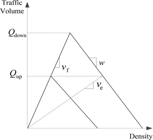
where, $Q_{\mathrm{up}}$ and $Q_{\mathrm{down}}$ are the traffic volume of upstream and downstream sections respectively.

It should be noted that the results of the numerical experiments show that using $v_e$ may cause an over-estimation of the queue dissipation time prediction under different queue length as shown in Table 1. In this case, we reduce the error by introducing a coefficient ϑ > 1 according to the relationship between the speed of the traffic flow, the time to dissipate and the length of the queue.

Table 1. Comparison of dissipation time under different conditions.

Vehicle queue length/m	Dissipation time/s		$\vartheta$
	with $v_e$	without $v_e$
100	16.0	12.0	1.33
150	23.8	18.8	1.27
200	32.3	26.3	1.23
250	40.0	33.8	1.18
300	53.9	41.7	1.29

Define $p_{\mathrm{e}}^{\text{offset}\mathrm{ }}(t^{\mathrm{\text{'}}}),t_{{\mathrm{s}}^{\mathrm{\text{'}}}}\le t^{\mathrm{\text{'}}}\le t_{{\mathrm{e}}^{\mathrm{\text{'}}}},$ as a linear section function with ϑ·$v_e$ as the slope, $t_{{\mathrm{s}}^{\mathrm{\text{'}}}}$ and $t_{{\mathrm{e}}^{\mathrm{\text{'}}}}$ are the start time and end time respectively. For the part of the offset trajectory after $P_{\mathrm{end}},$ just move them in time to connect$\mathrm{ }\delta$ with $p_{\mathrm{e}}^{\text{offset}\mathrm{ }}(t_{{\mathrm{e}}^{\mathrm{\text{'}}}}),$ and use $p_{{\mathrm{e}}^{\mathrm{\text{'}}}}^{\text{offset}\mathrm{ }}(t^{\mathrm{\text{'}}}),\forall t^{\mathrm{\text{'}}}\ge t_{{\mathrm{e}}^{\mathrm{\text{'}}}}$ to denote. Figure 4 shows the corrected offset trajectories $p_{\mathrm{e}}^{\text{offset}\mathrm{ }}(t^{\mathrm{\text{'}}})$ and $p_{{\mathrm{e}}^{\mathrm{\text{'}}}}^{\text{offset}\mathrm{ }}(t^{\mathrm{\text{'}}})$ and Figure 5 shows the basic triangle diagram with $v_e$ derivation.

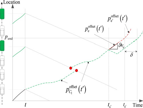
The offset trajectory obtained after the above steps is actually a set of functions. Since the information will be updated at each decision time point, they may overlap at some time points, causing interruptions, as shown in the red dot in Figure 4. The discontinuity of the predicted trajectory may cause obvious and unnatural fluctuations in the CAV control strategy. To construct a continuous prediction function $r(t\mathrm{\text{'}}),$ $\forall t\mathrm{\text{'}}\ge t,$ the algorithm proposed by Chen et al. (2021) is used to determine the merging points, and they are connected together to form a continuous function, as shown in Figure 6.

Figure 6. Connection merging points.

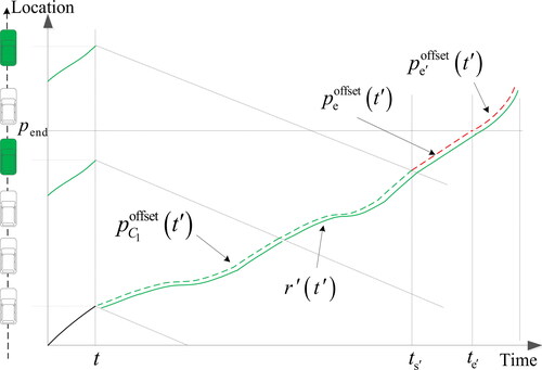
In addition, considering that the HV driver has a reaction time $\tau$ during the decelerated operation, the cumulative reaction time of multiple HVs will cause a certain error in the predicted trajectory. Therefore, for safety, the predicted trajectory function $r_{ti}(t^{\mathrm{\text{'}}}),\forall t^{\mathrm{\text{'}}}\ge t$ is adjusted by formula $r^{\mathrm{\text{'}}}(t^{\mathrm{\text{'}}})=r(t^{\mathrm{\text{'}}}-\tau )-s_0,\forall t\mathrm{\text{'}}\ge t,$ and finally the predicted HV trajectory function $r^{\mathrm{\text{'}}}\left(t^{\prime }\right),\forall t^{\mathrm{\text{'}}}\ge t$ is obtained, as shown by the solid line in Figure 7.

Figure 7. Modified offset trajectory.

5. Planning the speed of CAV

After predicting the trajectory of the vehicle ahead, it is necessary to plan the speed of the CAV. Since the setting scene is a single-lane straight section, the spatial trajectory planning is not considered, but the speed distribution at the time point is planned. The method of guiding the CAV to adjust the speed in a small range for a long time instead of a large deceleration in a short time is used to counter the reverse deceleration wave, reduce the propagation of speed oscillation, and make the upstream CAV vehicle cluster merge into the downstream traffic flow at a more reasonable speed. To ensure the comfort of the driver during the speed guidance process, it is also necessary to ensure the smoothness of the CAV’ speed to avoid sudden changes in acceleration.

Take a section of expressway as an example. It is stipulated that each vehicle cluster is led by the CAV. In the process of guiding the road section, the change curve of vehicle speed and position is shown in Figure 8, and the speed curve of HV is obtained according to the previous method. Considering that there may be different situations after the front HV speed rapidly reduced from high, such as continuing to run at a low speed for a long time. At this time, the following CAV can only be forced to take a long deceleration into the downstream queue and finally follow the leader within a safe distance. But the scenario designed in this section is the more common situation on the highway where the front HV suddenly decelerates and gradually returns to the normal speed in a short period of time. It is divided into three statuses as follow.

Figure 8. The first speed of CAV guidance process of the upstream vehicle cluster.

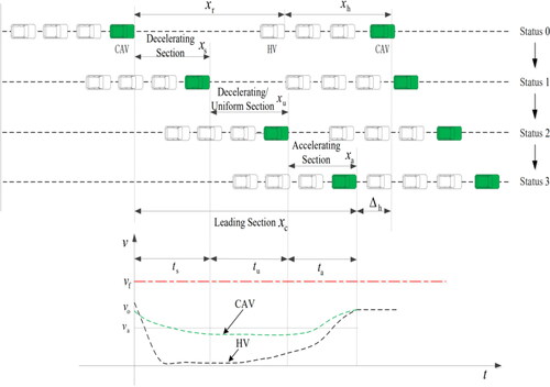
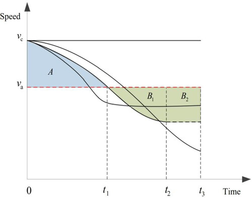
(1) Deceleration phase (status 0—status 1/2)

There are an infinite number of ways to accelerate from one speed to another speed including constant acceleration, linear-acceleration, and constant-throttle acceleration. All possible trajectories need to reach a specific point at specific time, therefore the area of region $A$ must be equal to the area of regions $B_1$ and $B_2$ as shown in Figure 9. In this way, we divide the guidance process of vehicle’s deceleration into three stages according to the time points. Compared with rapid deceleration, each scheme can reduce the fluctuation of the subsequent traffic flow and make the traffic flow more stable.

Figure 9. Deceleration curves.

To ensure smooth connection of trajectory and comfort of driver (i.e., low jerk), we choose a speed guidance model based on trigonometric function. Therefore, the piece-wise function is defined as follows: (16) $$v=\{\begin{array}{c}{v}_{\mathrm{a}}+v_d\text{cos}\left(\alpha t\right),\\ v_{\mathrm{a}}-\frac{\alpha }{\beta }{v}_d\text{cos}\beta \left(t-\frac{\pi }{2\alpha }+\frac{\pi }{2\beta }\right),\\ v_{\mathrm{a}}-\frac{\alpha }{\beta }{v}_d,\end{array}\begin{array}{cc}& 0\le t\le \frac{\pi }{2\alpha }\\ & \frac{\pi }{2\alpha }\le t\le \frac{\pi }{2\alpha }+\frac{\pi }{2\beta }\\ & \frac{\pi }{2\alpha }+\frac{\pi }{2\beta }\le t\le \frac{d}{v_{\mathrm{a}}}\end{array}$$(16)

In the equation, the parameters $\alpha$ and $\beta$ define the family of velocity profiles. Different values of ($\alpha ,\mathrm{ }\beta$) correspond to different acceleration and jerk profiles. Three piece-wise functions are used to describe the speed guidance process. $\left[0,\frac{\pi }{2\alpha }\right]$ is part of the time interval of CAV deceleration. In this process, the vehicle is reduced from the current speed to the average speed $v_{\mathrm{a}}$ of the interval, and the completion time is marked as $t_1;$ In the interval of $\left[\frac{\pi }{2\alpha },\frac{\pi }{2\alpha }+\frac{\pi }{2\beta }\right],$ the CAV continues to decelerate. During this process, the absolute value of the vehicle’s acceleration gradually decreases to zero, and starts at a constant speed at $t_2.$$\mathrm{ }\left[\frac{\pi }{2\alpha }+\frac{\pi }{2\beta },\frac{d}{v_{\mathrm{a}}}\right]$ is the time interval during which the CAV travels at a constant speed and arrives at a specific position at $t_3;$ $d$ is the distance from CAV to a specific location. With time $t_3$ and distance $d,$ the average vehicle’s speed of the entire deceleration guidance process can be obtained, that is, $v_{\mathrm{a}}= d$/$t_3,$ $v_{\text{d }}$ is the difference between the speed $v_{\mathrm{c}}$ at which the CAV starts speed guidance and the average speed $v_{\mathrm{a}},$ that is $v_{\text{d }}=v_{\mathrm{c}}-v_{\mathrm{a}}.$

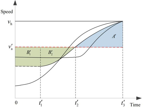
(2) Acceleration phase (status 2—status 3)

In the same way, to make the decelerated CAV merge into downstream at the recovered speed at a specific position and then follow the leader at a constant speed, the CAV needs to accelerate slightly in advance according to the remaining space headway. Similar to deceleration, there are also multiple acceleration trajectories to choose, as shown in Figure 10.

Figure 10. Acceleration curves.

The expression of the accelerated guidance model based on trigonometric function is selected as equation (17)(17) $$v=\{\begin{array}{c}{v}_{\mathrm{a}}^{\mathrm{\text{'}}}-v_d\text{cos}\left(\alpha t\right),0\le t\le t_1^{\mathrm{\text{'}}}\\ v_{\mathrm{a}}^{\mathrm{\text{'}}}-\frac{\alpha }{\beta }{v}_d\text{cos}\beta \left(t-\frac{\pi }{2\alpha }+\frac{\pi }{2\beta }\right),\mathrm{ }{t}_1^{\mathrm{\text{'}}}\le t\le t_2^{\mathrm{\text{'}}}\\ v_{\mathrm{a}}^{\mathrm{\text{'}}}+\frac{\alpha }{\beta }{v}_{d\mathrm{ }},{\mathrm{ }t}_2^{\mathrm{\text{'}}}\le t\le t_3^{\mathrm{\text{'}}}\end{array}\begin{array}{cc}& \\ & \\ & \end{array}$$(17) . (17) $$v=\{\begin{array}{c}{v}_{\mathrm{a}}^{\mathrm{\text{'}}}-v_d\text{cos}\left(\alpha t\right),0\le t\le t_1^{\mathrm{\text{'}}}\\ v_{\mathrm{a}}^{\mathrm{\text{'}}}-\frac{\alpha }{\beta }{v}_d\text{cos}\beta \left(t-\frac{\pi }{2\alpha }+\frac{\pi }{2\beta }\right),\mathrm{ }{t}_1^{\mathrm{\text{'}}}\le t\le t_2^{\mathrm{\text{'}}}\\ v_{\mathrm{a}}^{\mathrm{\text{'}}}+\frac{\alpha }{\beta }{v}_{d\mathrm{ }},{\mathrm{ }t}_2^{\mathrm{\text{'}}}\le t\le t_3^{\mathrm{\text{'}}}\end{array}\begin{array}{cc}& \\ & \\ & \end{array}$$(17)

Since the planned speed needs to ensure that the CAV can merge into the downstream queue from the current speed at a specific time and a specific position, thus the area of $A^{\prime }$ must be equal to the sum of areas $B_1^{\prime }$ and $B_2^{\prime },$ so the following equation can be obtained: (18) $${\int }_0^{t_1}{v}_d\hspace{0.17em}\text{cos}\hspace{0.17em}\left(\alpha t\right)dt={\int }_{t_1}^{t_2}\frac{\alpha }{\beta }{v}_d\hspace{0.17em}\text{cos}\hspace{0.17em}\beta \left(t-\frac{\pi }{2\alpha }+\frac{\pi }{2\beta }\right)dt+{\int }_{t_2}^{t_3}\frac{\alpha }{\beta }{v}_{d}dt,\mathrm{ }\mathrm{deceleration}$$(18) (19) $${\int }_{t_2^{\mathrm{\text{'}}}}^{t_3^{\mathrm{\text{'}}}}\frac{\alpha }{\beta }{v}_{d}dt={\int }_0^{t_1^{\mathrm{\text{'}}}}{v}_d\hspace{0.17em}\text{cos}\hspace{0.17em}\left(\alpha t\right)dt+{\int }_{t_1^{\mathrm{\text{'}}}}^{t_2^{\mathrm{\text{'}}}}\frac{\alpha }{\beta }{v}_d\hspace{0.17em}\text{cos}\hspace{0.17em}\beta \left(t-\frac{\pi }{2\alpha }+\frac{\pi }{2\beta }\right)dt,\mathrm{ }\text{acceleration}$$(19) where $\alpha 、\beta$ can be obtained by equation (18)(18) $${\int }_0^{t_1}{v}_d\hspace{0.17em}\text{cos}\hspace{0.17em}\left(\alpha t\right)dt={\int }_{t_1}^{t_2}\frac{\alpha }{\beta }{v}_d\hspace{0.17em}\text{cos}\hspace{0.17em}\beta \left(t-\frac{\pi }{2\alpha }+\frac{\pi }{2\beta }\right)dt+{\int }_{t_2}^{t_3}\frac{\alpha }{\beta }{v}_{d}dt,\mathrm{ }\mathrm{deceleration}$$(18) and equation (19)(19) $${\int }_{t_2^{\mathrm{\text{'}}}}^{t_3^{\mathrm{\text{'}}}}\frac{\alpha }{\beta }{v}_{d}dt={\int }_0^{t_1^{\mathrm{\text{'}}}}{v}_d\hspace{0.17em}\text{cos}\hspace{0.17em}\left(\alpha t\right)dt+{\int }_{t_1^{\mathrm{\text{'}}}}^{t_2^{\mathrm{\text{'}}}}\frac{\alpha }{\beta }{v}_d\hspace{0.17em}\text{cos}\hspace{0.17em}\beta \left(t-\frac{\pi }{2\alpha }+\frac{\pi }{2\beta }\right)dt,\mathrm{ }\text{acceleration}$$(19) : (20) $${\beta }^2+\alpha \beta (\frac{\pi }{2}-T\alpha )+{\alpha }^2(\frac{\pi }{2}-1)=0$$(20) where $T$ is the time required for the entire speed guidance process, and $T=\frac{2x_c}{v_a+v_{a^{\mathrm{\text{'}}}}}.$

Only when $\alpha \ge \frac{3.08}{T}\mathrm{ }\text{or}\mathrm{ }0\le \alpha \le \frac{0.06}{T},$ the equation has a real solution. Given a value of $\alpha ,$ the value of $\beta$ is: (21) $$\beta =\frac{1}{2}\left(\alpha \left(T\alpha -\frac{\pi }{2}\right)+\sqrt{{\alpha }^2{\left(\frac{\pi }{2}-T\alpha \right)}^2-4{\alpha }^2\left(\frac{\pi }{2}-1\right)}\right)\mathrm{ }$$(21)

The parameters $\alpha$ and $\beta$ determine the trajectory of the deceleration and acceleration curve. Parameter$\alpha$ controls the rate of change of speed in zone $A,$ and parameter $\beta$ controls the rate of change of speed in zone $B.$ In addition, considering the vehicle’s own performance, driver’s comfort and car-following safety factors, it is necessary to constrain the vehicle’s acceleration $a$ and jerk $\epsilon ,$ and the required safety distance $(\mathrm{\Delta }h-l_v)$ when approaching the leader, and the restored vehicle’s speed is less than the maximum lane speed limit $v_{\mathrm{f}},$ so the constraint conditions are: (22) $$\{\begin{array}{c}\left|{\mathrm{\epsilon }}_{\max }\right|=v_d\alpha \beta \le 10 m/{\mathrm{s}}^3\\ \left|a_{\max }\right|\le 2.5 m/{\mathrm{s}}^2\\ x_{\mathrm{r}}+x_{\mathrm{h}}-x_{\mathrm{c}}=\Delta h>\frac{v^2}{2a}+l_{\mathrm{v}}\\ v\le v_{\mathrm{f}}\end{array}$$(22)

Through the above solution and constraint conditions, a feasible and smooth guided curve of velocity can be obtained. It should be noted that when the distance between the preceding HV and the CAV is relatively close, and the curve does not meet the safety constraints with the preceding vehicle, the random OV car-following model is used to guide the speed of the CAV.

6. Numerical simulation analysis

To evaluate the rationality of the strategy, we use Matlab to build a simulation environment and conduct numerical experiments. First, we set the starting position $l_{B }$ of the bottleneck at 575 m, and deploy a group of road side sensors around $l_B.$ The other default parameter values are set as: the number of road side sensors $S$ is 7, the update frequency of decision time$\mathrm{ }\mathrm{\Delta }T$ is 2 s, the speed limit $v_{\mathrm{f}}$ is 120 km/h, the driver response time $\tau$ is set as 0.65 s, the speed of traffic wave $w$ is 4.64 m/s, ϑ = 1.25, $s_0$= 6.5 m and $P_{\mathrm{end}}=l_s.$ It is assumed that each traffic sensor can capture traffic information within 200 meters (that is, a coverage area of 400 meters) from its center. For all numerical experiments, let HVs and AVs follow the random optimal velocity (OV) car-following model and the volume of a single lane is set to 1440 pcu/h for numerical experiments.

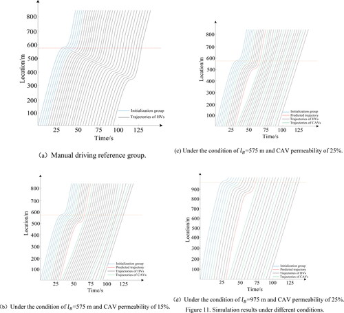
To provide historical information to the road side sensor, a set of 5 vehicles were used to initialize the simulation, which is shown by the blue curves in the Figure 11. In addition, HVs and CAV are displayed in black and green curves respectively. In addition, the red curves are the HV trajectories predicted based on the CAVs trajectories and road side sensors information in the same cluster. It should be noted that CAV follows the planned speed to a decision point, then the planned speed will be updated. To compare the results, a reference group was constructed, which simulated a manual traditional vehicle without any control. Figure 11(a) shows the traditional vehicle trajectories generated by the random OV model, and compares it with the result of the established speed coordination strategy, as shown in Figure 11(b)–(d).

Figure 11. Simulation results under different conditions.

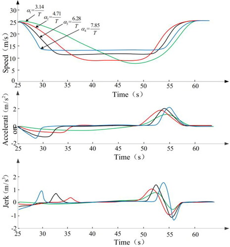
It should be noted that after CAV predicting the downstream trajectory of HV, there are multiple ways to plan CAV’s speed trajectory to smoothly merge into the traffic flow at a specific downstream location. As mentioned above, this depends on the value of parameter $\alpha$ and $\beta .$ Figure 12 shows the speed curves corresponding to several different values of $\alpha .$ These several methods can suppress the spread of traffic oscillations to a certain extent. To ensure the comfort of the driver as much as possible, we choose the smoothest speed curve in the whole coordination process, that is, the speed curve with the smallest average jerk to guide the first CAV of the upstream vehicle cluster, that is the green line in Figure 12.

Figure 12. Several different speed guide curves.

7. Discussion

Comparing Figure 11(a) and (b), it can be found that the upstream CAV can adjust its speed well in this process. Therefore, the CAV cluster can suppress the traffic oscillation by hedging the deceleration wave to a certain extent, and make itself gradually and smoothly merge into the downstream traffic flow. Comparing Figure 11(b) and (c), it can be found that the permeability of CAV in the vehicle cluster will affect the degree of restraining traffic oscillation, that is to say, the higher the CAV permeability, the earlier the vehicle cluster reaches steady state. To further study, the influence of different CAV permeability on the traffic efficiency in the same speed coordination mode, the same number of simulated vehicles are collected here, and the time taken by the tail cars to travel to different distances is taken as the evaluation index. The results show: The travel time of the vehicle queue decreases with the increase of CAV permeability. When the permeability reaches 25%, the travel time can be reduced by 7.10%, as shown in Table 2. It can be seen that the designed speed coordination strategy can reduce the travel time by suppressing traffic oscillation and thus improve the transit efficiency.

Table 2. The time of the last vehicle to reach the same position under different CAV permeability.

CAV Permeability/%	Time (s)			Reduction rate /%
	500 m	600 m	700 m
0 (Reference Group)	125.1	129.2	133.2	–
5	123.9	127.5	131.8	1.16
10	121.4	125.3	129.5	2.90
15	119.5	123.6	127.4	4.41
20	117.6	121.6	125.5	5.90
25	115.5	120.2	124.3	7.10

In addition, comparing Figure 11(c) and (d), it can be found that under the same CAV permeability, the difference between the starting position of the bottleneck and the CAV also affects the degree of suppression of traffic oscillation. Table 3 shows the acceleration value of the first upstream CAV vehicle in 30 s∼70 s corresponding to different $l_B$ values under the 20% CAV permeability. The analysis result shows that: In the same time range, the larger the value of $l_B,$ the smaller the most value difference of acceleration, the smaller the fluctuation of acceleration, and the smoother the running of the vehicle cluster it guides. The reason may be that for a larger value of $l_B,$ CAV has more space and time to adjust its own speed after predicting the trajectory of preceding HV to make the traffic oscillation smaller and the speed’s trajectory smoother.

Table 3. Acceleration of the first CAV at different time corresponding to different $l_B$ values.

Timing	Acceleration at different locations at the beginning of the bottleneck (m/s^2)
	575 m	775 m	975 m
30s	−0.25	−0.18	−0.13
35s	−0.42	−0.21	−0.05
40s	−0.68	−0.34	−0.02
45s	−0.41	−0.23	0.00
50s	0.09	0.05	0.02
55s	1.63	1.22	0.06
60s	0.16	0.07	0.04
65s	0.08	0.05	0.02
70s	0.04	0.02	0.01
The most value difference	2.31	1.56	0.19

8. Conclusion

With the help of vehicle-vehicle and vehicle-road collaboration technology, the trajectory of downstream HV can be well predicted within a certain period of time. The coordinated control of CAV’s speed based on the predicted trajectory can make the vehicle cluster of this vehicle smoothly converge into the downstream traffic flow at a reasonable speed.

Research indicates: Coordinated control of speed can restrain the propagation of traffic oscillations, and the degree of restraint is related to the permeability of the CAV in the vehicle cluster, the starting position of the bottleneck, and the speed’s trajectory selected by the CAV. In general, when the designed CAV permeability is 0%∼25% and 575 m<$l_B$<975 m, the higher the permeability, the farther the bottleneck starting position $l_B,$ the smoother the planning speed selected by CAV, and the more obvious the degree of suppression of oscillation. This will effectively improve the efficiency of vehicle queues, the safety and comfort of drivers.

The research reveals the great potential of the coordinated strategy of vehicle’s speed in the context of the new intelligent network technology to improve the stability of traffic flow. The proposed strategy is currently mainly aimed at the single-lane scene of the expressway. In real traffic situations, the surrounding vehicles can influence car-following behavior. A typical event is the cut-in, which results in considerable fluctuations in the cooperative adaptive cruise control queue. It is undeniable that the application scenario of the algorithm is still limited. In the follow-up research, we need to improve the algorithm by establishing a car-following model of CAV that can adapt to various situations, which will be the next theme we need to study.

Acknowledgments

Dayi Qu and Yanfeng Jia conceived and designed the research. We thank Dr. Tao Wang for the help in experiments and data analysis. Comments from Dr. Bin Li and Lewei Han significantly improved this manuscript. All authors read and approved the final manuscript.

Disclosure statement

No potential conflict of interest was reported by the author(s).

Data availability statement

The data used to support the findings of this study are available from the corresponding author upon request.

Additional information

Funding

The study is supported by the National Natural Science Foundation of China (No. 51678320).

References

- Ahn, S., & Cassidy, M. J. (2007). Freeway traffic oscillations and vehicle lane-change maneuvers. Transportation and Traffic Theory, 1, 691–710.
- Chen, P., Wang, T., & Zheng, N. (2021). Reconstructing vehicle trajectories on freeways based on motion detection data of connected and automated vehicles. Journal of Intelligent Transportation Systems, 1–16. https://doi.org/10.1080/15472450.2021.1955211
- Ghiasi, A., Hussain, O., Qian, Z. S., & Li, X. (2017). A mixed traffic capacity analysis and lane management model for connected automated vehicles: A Markov chain method. Transportation Research Part B: Methodological, 106, 266–292. https://doi.org/10.1016/j.trb.2017.09.022
- Guo, Y., Ma, J., Xiong, C., Li, X., Zhou, F., & Hao, W. (2019). Joint optimization of vehicle trajectories and intersection controllers with connected automated vehicles: Combined dynamic programming and shooting heuristic approach. Transportation Research Part C: emerging Technologies, 98, 54–72. https://doi.org/10.1016/j.trc.2018.11.010
- Han, Y., Chen, D., & Ahn, S. (2017). Variable speed limit control at fixed freeway bottlenecks using connected vehicles. Transportation Research Part B: Methodological, 98, 113–134. https://doi.org/10.1016/j.trb.2016.12.013
- Kattan, L., Khondaker, B., Derushkina, O., & Poosarla, E. (2015). A probe-based variable speed limit system. Journal of Intelligent Transportation Systems, 19(4), 339–354. https://doi.org/10.1080/15472450.2014.936294
- Laval, J. A. (2007). Linking synchronized flow and kinematic waves. In Traffic and Granular Flow (Vol. 5, 521–526). Springer.
- Laval, J. A., & Daganzo, C. F. (2006). Lane-changing in traffic streams. Transportation Research Part B: Methodological, 40(3), 251–264. https://doi.org/10.1016/j.trb.2005.04.003
- Laval, J. A., & Leclercq, L. (2010). A mechanism to describe the formation and propagation of stop-and-go waves in congested freeway traffic. Philosophical Transactions. Series A, Mathematical, Physical, and Engineering Sciences, 368(1928), 4519–4541. https://doi.org/10.1098/rsta.2010.0138
- Li, X., Wang, X., & Ouyang, Y. (2012). Prediction and field validation of traffic oscillation propagation under nonlinear car-following laws. Transportation Research Part B: Methodological, 46(3), 409–423. https://doi.org/10.1016/j.trb.2011.11.003
- Motamedidehkordi, N., Margreiter, M., & Benz, T. (2016). Shockwave suppression by vehicle-to-vehicle communication. Transportation Research Procedia, 15, 471–482. https://doi.org/10.1016/j.trpro.2016.06.040
- Pang, M., & An, S. (2019). Dispersive lane change and speed guidance method for expressways and adjacent intersections. Journal of Transportation Systems Engineering and Information Technology, 19(6), 168–175.
- Qin, Y., Wang, H., & Ran, B. (2021). Impacts of cooperative adaptive cruise control platoons on emissions under traffic oscillation. Journal of Intelligent Transportation Systems, 25(4), 376–383. https://doi.org/10.1080/15472450.2019.1702534
- Qin, Y. Y., Wang, H., & Wang, W. (2018). LWR model for mixed traffic flow in connected and autonomous vehicular environments. China Journal of Highway and Transport, 31, 147–156.
- Soriguera, F., Martínez, I., Sala, M., & Menéndez, M. (2017). Effects of low speed limits on freeway traffic flow. Transportation Research Part C: Emerging Technologies, 77, 257–274. https://doi.org/10.1016/j.trc.2017.01.024
- Wang, M., Daamen, W., Hoogendoorn, S. P., & van Arem, B. (2016). Connected variable speed limits control and car-following control with vehicle-infrastructure communication to resolve stop-and-go waves. Journal of Intelligent Transportation Systems, 20(6), 559–572. https://doi.org/10.1080/15472450.2016.1157022
- Wang, P., Jiang, Y., Xiao, L., Zhao, Y., & Li, Y. (2020). A joint control model for connected vehicle platoon and arterial signal coordination. Journal of Intelligent Transportation Systems, 24(1), 81–92. https://doi.org/10.1080/15472450.2019.1579093
- Wang, P., Yu, H., & Zhang, W. (2019). Reak-time traffic status evaluation method for urban cooperative vehicle infrastructure system. China Journal of Highway and Transport, 32(6), 176–187.
- Zhao, W., Ngoduy, D., Shepherd, S., Liu, R., & Papageorgiou, M. (2018). A platoon based cooperative eco-driving model for mixed automated and human-driven vehicles at a signalised intersection. Transportation Research Part C: Emerging Technologies, 95, 802–821. https://doi.org/10.1016/j.trc.2018.05.025
- Zheng, Z., Ahn, S., Chen, D., & Laval, J. (2011). Freeway traffic oscillations: Microscopic analysis of formations and propagations using wavelet transform. Procedia - Social and Behavioral Sciences, 17, 702–716. https://doi.org/10.1016/j.sbspro.2011.04.540