Modeling and simulation of dynamic lane reversal using a cell transmission model

Abstract

In recent years, large-scale testing has begun for connected and autonomous driving, making it possible to implement the concept of Dynamic Lane Reversal (DLR), which can quickly shift lane directions to reflect instantaneous flow dynamics. DLR is to make full use of road space and avoid waste of road capacity, and potentially alleviate congestion. However, the impact and feasibility of DLR remain unclear. In order to investigate the effectiveness, the feasibility, and the applicability of DLR, we utilize a direction-changeable, lane-based cell transmission model to find an optimal DLR scheme for a roadway segment with stochastic traffic flow in both directions. A proxy model is also designed to realize DLR in VISSIM. A regression analysis was carried out to find the impacts of directional flow rate and the number of lanes on delay reductions due to DLR. Results indicate that implementing DLR can reduce the total queuing delay considerably compared to traditional reversible lane strategies. We found that DLR achieved superior performance on segments with more lanes and when the flows from each direction were close to one another. A zigzag frontier of the delay reduction was discovered. Findings from this research shed light on the feasibility and effectiveness of DLR on various types of road segments.

Keywords:

• Cell transmission model
• dynamic lane reversal
• multi-objective optimization
• VISSIM

Introduction

Increases in the total amount of commuting traffic, travel distance during peak hours and the number of urban vehicles has led to tidal phenomenon on urban roads, especially on corridors connecting workplaces and residential areas. There are many measures for integrated corridor management and evacuation (Tian & Chiu, 2014). Establishing reversible lanes is an operational strategy that can improve road efficiency without widening the road, which can effectively alleviate congestion by making full use of every lane.

The Golden Gate Bridge in San Francisco, for example, has six lanes that are crossed by 3 million vehicles every month. Reversible lanes were installed there more than half a century ago. Road workers move lane markers to show drivers the direction of each lane (Agent & Clark, 1982). Currently, the real-world implementation of reversible lanes is mainly done manually or by road zippers and removable barriers. The speed of a typical road zipper is around 10 km/h. Due to limitations of facilities and vehicles’ lane changing ability, reversible lanes are typically operated on regular fixed schedules at hours that reflect daily commute and traffic patterns.

The emergence of Connected and Autonomous Vehicles (CAVs) has the potential to reshape the idea of reversible lanes. A CAV is defined as a vehicle that can sense its environment, receive real-time information from road-side units or other vehicles, and move safely and intelligently with little or no human input (Xie et al., 2017). With full deployment of CAVs on public roads in the future, lane reversal information can be transmitted to all vehicles through V2X or V2V devices immediately (Claes et al., 2011). Furthermore, autonomous driving modules can enact the decisions and actions involved in lane changing operations.

In an ideal scenario with 100% CAV penetration, lane markers are no longer required on roads, and CAVs can drive freely and safely (Bansal & Kockelman, 2017). Therefore, with the connectivity and automation capabilities of CAVs, the idea of Dynamic Lane Reversal (DLR), which alters the lane directions of road segments to reflect instantaneous lane occupancies and flow dynamics, can be implemented. The practical purpose of DLR is to make full use of road space and avoid waste of lane capacity. Such frequent reversals of lane direction in DLR can be used to meet variations in traffic demand over time, when CAV reaches 100% penetration.

However, there are substantial difficulties related to the deployment of DLR. First, it will take decades for the penetration of CAVs to reach 100%. Second, to the best of the authors’ knowledge, no research effort has been devoted to CAV control in a DLR situation with high frequency lane direction changes. Finally, the process of moving from a typical roadway segment to a DLR one is presumably costly. In a possible DLR scenario, aside from all vehicle related expenses, the framework requires Road Side Units (RSUs) that are capable of detecting real time directional occupancies and disseminating lane direction information. Thus, in circumstances with a limited facility budget, administrators need to prioritize certain roads to remodel and should implement DLR on roads that lead to the largest travel time savings.

Some of the possible factors that intuitively may impact the effectiveness of DLR include the bidirectional flow pattern and the number of lanes. Kim and Shekhar (2005 November) demonstrated that flow is an important factor in determining the direction of the road in their study of fixed-schedule reversible lanes. Hausknecht et al. (2011) found that when one of the directions is oversaturated while the other is undersaturated, the effectiveness of reversible lanes is more obvious. Additionally, intuitively speaking, the more lanes there are, the more likely DLR is to be discrete. The more possible states DLR has, the better performance it might achieve. As such, it is necessary to explore the relationship between the bidirectional flow pattern, the number of lanes and the effectiveness of DLR.

Existing studies on fixed-schedule reversible lanes have direction changing periods of 1-6 hours (Claes et al., 2011; Gershenson & Rosenblueth, 2012; Goel et al., 2017). As noted by Hausknecht et al. (2011), without consideration of vehicle safety, more frequent lane direction switches leads to performance improvements. Scenarios with frequencies as high as 1/6 Hz have been numerically simulated (Levin & Boyles, 2016). However, the relationship between frequency and performance improvements has not been thoroughly modeled. It remains unclear whether the performance of DLR remains the same in sophisticated simulation models.

To address the aforementioned research questions, this study aims to prospectively investigate the technical feasibility and layout proposal of DLR under the assumption that CAV technology is mature and can be practically implemented with a 100% penetration rate. We investigate factors that potentially influence the effectiveness of DLR. We examine DLR with a high direction change frequency, which can potentially lead to higher travel time savings. The DLR strategy of interest can operate at frequencies as high as 1/6 Hz.

We take the following steps. First, we established a multi-objective optimization model based on a Cell Transmission Model (CTM). Using a genetic algorithm, we solved for the optimal DLR control scheme under different traffic and lane configuration conditions. Second, since the impact of lane changing cannot be depicted explicitly in a CTM, we further verified the feasibility of the optimal DLR scheme in VISSIM. A dedicated proxy model was designed in VISSIM to enable a DLR scenario. Third, using regression analysis, we examined the relationship between flow-efficiency improvement and potential influencing factors including the number of lanes and the directional flow rate.

This study contributes to the field of DLR by assessing the influence of various factors on the effectiveness of DLR. The results serve to help local agencies select the most suitable roads for DLR implementation. Our results also shed light on the design and communication frequency of CAVs when incorporating DLR in the future.

The remainder of this paper is organized as follows: Literature review discusses previous work on DLR and CTM. Methods presents the methodology. Results and discussion details the simulation results, and Conclusion concludes this paper.

Literature review

Many studies have explored the applications and feasibility of conventional lane reversal strategies. Most reversible lanes are usually set up with a fixed timing scheme based on analysis of historical data or are controlled by traffic police according to situations on site (Ampountolas et al., 2020; Ampountolas & Carlson, 2019; Liu et al., 2019; Sangho et al., 2008). For example, Zhou et al. (1993) developed reversible lane control systems for managing the George Massey tunnel. The time interval of lane reversal was consistent with the peak traffic hours in the morning and evening, which were both more than one hour. The control frequency of these schemes is low and these approaches are unable to cope with traffic flow changes satisfactorily (Gershenson & Rosenblueth, 2012). The frequencies of these systems are greatly lower than that of real-time adaptive control systems widely used at signalized intersections (Goel et al., 2017).

In terms of actuated timing schedule, Hausknecht et al. (2011) proposed a theoretical scheme in a situation with automated vehicles. They used integer linear programming, bi-level programming, and a genetic algorithm to prove the practicality of an actuated timing schedule in traffic management. Dey et al. (2011) established an actuated lane direction control model and classified the control model based on the bidirectional saturation of the lanes. They found that dynamically controlling the lane direction effectively reduced the average delay and alleviated road traffic congestion under certain conditions. While those works afford technical merits, they suffer from the following drawbacks. First, the time intervals of lane reversal in both works were roughly 1.5 hours, which is too high to fully utilize the potential advantages of DLR. Additionally, the model and solution methods corresponded with specific traffic conditions. If slight changes occurred in these traffic conditions, these approaches would need to be remodeled.

Switching lane directions frequently is not an issue with the help of changeable markers, but these devices are anticipated to be expensive. Besides, rapid changes in lane directions may confuse human drivers. The appearance of CAVs helps vehicles adjust to rapid changes in lane direction. Aided by CAV technology, more aggressive lane reversal strategies will become possible. As reported by (Chu et al., 2020), CAVs can complete the entire lane changing process in 6 seconds, meaning that lane directions can be switched every 6 seconds in a DLR scheme if CAV penetration reaches 100%.

The original CTM was developed by Daganzo as a discrete approximation of the hydrodynamic theory of traffic flow (Daganzo, 1994, 1995). Currently, some scholars have applied CTMs to investigate the feasibility of reversible lanes. For example, Levin and Boyles (2016) presented a cell transmission model formulation of DLR and introduced the theoretical conditions that need to be considered. However, the factors affecting the improvement of DLR when compared to the status quo remain unclear.

To conclude, there is no research on the simulation and validation of DLR in sophisticated simulation models. Furthermore, it remains unclear as to where DLR should be implemented first, given that the influence of various factors (incoming directional flow, update frequency, number of lanes, etc.) is unknown.

Methods

We aim to investigate the influencing factors impacting the delay improvement of DLR in a CAV environment in order to determine roads that should be prioritized for DLR implementation. To achieve this, we take the following steps.

First, we adopt the Nondominated Sorting Genetic Algorithm II (NSGA-II) to solve for an optimal DLR scheme configuration in the context of a CTM. Considering the effectiveness of DLR and the safety of CAVs, minimizing delay and the driving safety hazard index were set as objectives, and the Pareto frontier of optimal solutions was obtained.

Second, since the evolution of traffic flow as well as the propagation and dissipation of congestion is simplified in a CTM, we further implement a proxy model in VISSIM to test the functionality of DLR, which cross-validates the accuracy of the optimal DLR scheme found using the CTM.

Third, regression analysis is performed to find the statistical impact of potential influencing factors on the effectiveness of the optimal DLR scheme. The results help shed light on DLR implementation priority.

Implementation of CTM

CTMs can realize a macroscopic simulation of lane changes in DLR and describe macroscopic traffic phenomenon such as shockwaves and queue formation and dissipation. CTMs can also be used for the study of supersaturated traffic flow, which is compatible with our research. Therefore, a CTM model was chosen as the network loading model in this study.

The original CTM was developed by Daganzo (1994) as a discrete approximation of traffic flow hydrodynamics theory. Lane direction changes are achieved by modifying the definition of cells in the CTM. In our model, the road was divided into several modules that contain parallel but opposing lanes. The time horizon was divided into intervals with identical length Δt, and the states of the modules (such as capacity, inflow capacity, etc.) were altered as time evolved. With this, the continuous traffic flow was discretized. In order to prevent vehicles from traversing multiple modules within one time interval, the module lengths were set as the distance traveled in a time step at the free flow speed.

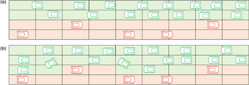
An example of DLR is shown in Figure 1. The red area indicates the forward direction of the module, and the green area indicates the backward direction of the module. The number of lanes in each direction within one module changes during each time interval if necessary. For instance, in the depiction below, the lane configuration shifts from the situation shown in Figure 1(a) to the one shown in Figure 1 (b).

Figure 1. Shift of Lane Directions in DLR. (a) Initial lane configuration. (b). Lane configuration in the next time interval.

According to the law of conservation of flow ∂q/∂x=-∂k/∂t, the state renewal equation and flow transfer equation for the forward direction in the CTM are given by the following Eq:(1)-(4): (1) $${\mathrm{n}}_{\mathrm{i}}\left(\mathrm{t}+1\mathrm{ }\right)={\mathrm{n}}_{\mathrm{i}}\left(\mathrm{t}\right)-{\mathrm{y}}_{\mathrm{i}+1}\left(\mathrm{t},\mathrm{L}\right)+{\mathrm{y}}_{\mathrm{i}}\left(\mathrm{t},\mathrm{L}\right)$$(1) (2) $${\mathrm{y}}_{\mathrm{i}}\left(\mathrm{t},\mathrm{L}\right)=\min \left\{{\mathrm{S}}_{\mathrm{i}-1}\left(\mathrm{t},\mathrm{L}\right),{\mathrm{R}}_{\mathrm{i}}\left(\mathrm{t},\mathrm{L}\right)\right\}$$(2) (3) $${\mathrm{S}}_{\mathrm{i}}\left(\mathrm{t},\mathrm{L}\right)=\min \left\{{\mathrm{n}}_{\mathrm{i}}\left(\mathrm{t}\right),{\mathrm{Q}}_{\mathrm{i}}\left(\mathrm{t}\right){\mathrm{L}}_{\mathrm{i}}\left(\mathrm{t}\right)\right\}$$(3) (4) $${\mathrm{R}}_{\mathrm{i}}\left(\mathrm{t},\mathrm{L}\right)=\min \left\{{\mathrm{Q}}_{\mathrm{i}}\right(\mathrm{t}\left){\mathrm{L}}_{\mathrm{i}}\right(\mathrm{t}),\mathrm{\delta }({\mathrm{N}}_{\mathrm{i}}\left(\mathrm{t}\right){\mathrm{L}}_{\mathrm{i}}\left(\mathrm{t}\right)-{\mathrm{n}}_{\mathrm{i}}\left(\mathrm{t}\right)\left)\right\}$$(4)

Where q denotes the flow and k denotes the density. ${\mathrm{n}}_{\mathrm{i}}\left(\mathrm{t}+1\right)\mathrm{ }$ denotes the number of vehicles moving in the forward direction of module i at time t + $1.$$\mathrm{ }{\mathrm{y}}_{\mathrm{i}}(\mathrm{t})$ denotes the number of incoming vehicles in this direction of module i at time t. ${\mathrm{S}}_{\mathrm{i}}\left(\mathrm{t},\mathrm{L}\right)$ denotes the outflow in this direction of module i at time t. ${\mathrm{R}}_{\mathrm{i}}\left(\mathrm{t},\mathrm{L}\right)\mathrm{ }$ denotes the acceptable flow in this direction of module i at time t. ${\mathrm{n}}_{\mathrm{i}}\left(\mathrm{t}\right)$ denotes the number of vehicles in this direction of module i at time t. ${\mathrm{L}}_{\mathrm{i}}(\mathrm{t})$ denotes the number of lanes in this direction of module i at time t. $\mathrm{\delta }$ denotes the congestion adjustment coefficient (if ${\mathrm{n}}_{\mathrm{i}-1}\left(\mathrm{t}\right)>{\mathrm{Q}}_{\mathrm{i}}(\mathrm{t}),$ $\mathrm{\delta }=\frac{\mathrm{w}}{\mathrm{v}},$ otherwise $\mathrm{\delta }=1,$ $\mathrm{w}$ is the speed of the backward motion wave, and v is the free flow speed). ${\mathrm{N}}_{\mathrm{i}}(\mathrm{t})$ denotes the maximum number of vehicles that each lane of module i can hold, and ${\mathrm{Q}}_{\mathrm{i}}(\mathrm{t})$ denotes the capacity flows of each lane of module i (which is equal to maximum number of vehicles that can flow into each lane of module i when the clock advances from t to t + 1).

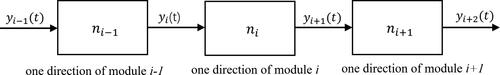
Eq. (1)-(4) represent the basic ideas of the CTM: the number of vehicles in the forward direction of module i at time t + 1 is equal to the number of vehicles in this direction of module i at time t plus the net incoming flow at time t + 1 (net incoming flow is equal to inflow minus outflow). Similarly, this same situation applies to the number of vehicles departing in the backward direction of module i (see Figure 2).

Figure 2. Traffic flow in the CTM.

In addition, the number of lanes in the modules changes dynamically, resulting in an inconsistent number of lanes before and after, which causes vehicles to change lanes frequently. This results in a decrease in the maximum capacity flows ${\mathrm{Q}}_{\mathrm{i}}^{\mathrm{\text{'}}}\left(\mathrm{t}\right).$ Therefore, the capacity correction factor $\mathrm{\alpha }$ was adopted to offset the impact of frequent lane changes in DLR. As such, the modified capacity flows ${\mathrm{Q}}_{\mathrm{i}}^{\mathrm{\text{'}}}\left(\mathrm{t}\right)$ of the modules was determined with Eq. (5)(5) $${\mathrm{Q}}_{\mathrm{i}}^{\mathrm{\text{'}}}\left(\mathrm{t}\right)={\mathrm{Q}}_{\mathrm{i}}\left(\mathrm{t}\right)\times \mathrm{\alpha }$$(5) . (5) $${\mathrm{Q}}_{\mathrm{i}}^{\mathrm{\text{'}}}\left(\mathrm{t}\right)={\mathrm{Q}}_{\mathrm{i}}\left(\mathrm{t}\right)\times \mathrm{\alpha }$$(5)

Some researchers have investigated the influence of the number of lanes in merging and diverging areas on road capacity and obtained a capacity correction coefficient table (Zheng et al., 2018). We regard the lane change behavior to be the same as merging and diverging behavior. Therefore, we adopted the capacity correction coefficient table suggested by Zheng et al. (2018) (See Table 1).

Table 1. Correction coefficients.

Parameters	Value
Number of Lanes	1	2	3	4
Correction Coefficient	1.000	0.982	0.965	0.947

Problem formulation

The ultimate goal of DLR is to fully utilize the existing spatial and temporal capacity of roadways while eliminating possible collisions due to frequent lane direction changes. Therefore, the delay (representing efficiency) and the driving safety hazard index (representing safety) are selected as the two objectives for the optimal control problem.

The CTM records vehicle delays in each module, and the delays are defined as the time taken for all vehicles to pass through the roadway minus the free-flow travel time. The vehicle delay in the forward direction of a module is given by Eq. (6)(6) $${\mathrm{d}}_{\mathrm{i}}\left(\mathrm{t}\right)=\left[{\mathrm{n}}_{\mathrm{i}}\left(\mathrm{t}\right)-{\mathrm{q}}_{\mathrm{i}+1}\left(\mathrm{t}\right)\right]△\mathrm{t}$$(6) , and the total delay can be determined using Eq. (7)(7) $$\mathrm{D}=\sum _{\mathrm{t}}\sum _{\mathrm{i}}\left[{\mathrm{d}}_{\mathrm{i}}\right(\mathrm{t})+{\mathrm{d}}_{\overleftarrow{\mathrm{i}}}(\mathrm{t}\left)\right]$$(7) : (6) $${\mathrm{d}}_{\mathrm{i}}\left(\mathrm{t}\right)=\left[{\mathrm{n}}_{\mathrm{i}}\left(\mathrm{t}\right)-{\mathrm{q}}_{\mathrm{i}+1}\left(\mathrm{t}\right)\right]△\mathrm{t}$$(6) (7) $$\mathrm{D}=\sum _{\mathrm{t}}\sum _{\mathrm{i}}\left[{\mathrm{d}}_{\mathrm{i}}\right(\mathrm{t})+{\mathrm{d}}_{\overleftarrow{\mathrm{i}}}(\mathrm{t}\left)\right]$$(7)

Where ${\mathrm{d}}_{\mathrm{i}}\left(\mathrm{t}\right)$ is the total vehicle delay for the forward direction in module i at time t and$\mathrm{ }{\mathrm{d}}_{\overleftarrow{\mathrm{i}}}\left(\mathrm{t}\right)$ is the total vehicle delay for the backward direction in module i at time t.

The frequent lane direction changes will lead to frequent vehicle lane-changings and sudden stops, and further lead to more occurrence of possible collisions. In order to ensure the traffic safety in circumstance of DLR, the safety hazard index β which is defined based on the number of lane direction changes is introduced, and it’s defined by Equation (8)(8) $$\mathrm{\beta }=\mathrm{ }\sum _{\mathrm{t}}\sum _{\mathrm{i}}\left|{\mathrm{L}}_{\mathrm{i}}\left(\mathrm{t}\right)-{\mathrm{L}}_{\mathrm{i}+1}\left(\mathrm{t}\right)\right|$$(8) : (8) $$\mathrm{\beta }=\mathrm{ }\sum _{\mathrm{t}}\sum _{\mathrm{i}}\left|{\mathrm{L}}_{\mathrm{i}}\left(\mathrm{t}\right)-{\mathrm{L}}_{\mathrm{i}+1}\left(\mathrm{t}\right)\right|$$(8)

Where ${\mathrm{L}}_{\mathrm{i}}\left(\mathrm{t}\right)$ is the number of lanes in the forward direction for module i at time t.

In order to minimize the two indicators mentioned above, i.e., the vehicle delay and the driving safety hazard index, a bi-objective programming model was formulated as follows. (9) $$\min \text{average delay}=\frac{\mathrm{D}}{\mathrm{M}}$$(9) (10) $$\text{min β}=\sum _{\mathrm{t}}\sum _{\mathrm{i}}\left|{\mathrm{L}}_{\mathrm{i}}\left(\mathrm{t}\right)-{\mathrm{L}}_{\mathrm{i}+1}\left(\mathrm{t}\right)\right|$$(10) (11) $$\mathrm{s}.\mathrm{t}.{\mathrm{y}}_{\mathrm{i}}\left(\mathrm{t},\mathrm{L}\right)=\min \left\{{\mathrm{S}}_{\mathrm{i}-1}\left(\mathrm{t},\mathrm{L}\right),{\mathrm{R}}_{\mathrm{i}}\left(\mathrm{t},\mathrm{L}\right)\right\}$$(11) (12) $${\mathrm{S}}_{\mathrm{i}}\left(\mathrm{t},\mathrm{L}\right)=\min \left\{{\mathrm{n}}_{\mathrm{i}}\left(\mathrm{t}\right),\mathrm{Q}{\mathrm{L}}_{\mathrm{i}}\left(\mathrm{t}\right)\right\}$$(12) (13) $${\mathrm{R}}_{\mathrm{i}}\left(\mathrm{t},\mathrm{L}\right)=\min \left\{\mathrm{Q}{\mathrm{L}}_{\mathrm{i}}\left(\mathrm{t}\right),\mathrm{\delta }\left({\mathrm{N}}_{\mathrm{i}}\left(\mathrm{t}\right){\mathrm{L}}_{\mathrm{i}}\left(\mathrm{t}\right)-{\mathrm{n}}_{\mathrm{i}}\left(\mathrm{t}\right)\right)\right\}$$(13) (14) $$\left|{\mathrm{L}}_{\mathrm{i}}\left(\mathrm{t}\right)-{\mathrm{L}}_{\mathrm{i}}\left(\mathrm{t}+1\right)\right|\le {\mathrm{L}}_{\mathrm{a}}$$(14) (15) $$\left|{\mathrm{L}}_{\mathrm{i}}\left(\mathrm{t}\right)-{\mathrm{L}}_{\mathrm{i}+1}\left(\mathrm{t}\right)\right|\le {\mathrm{L}}_{\mathrm{b}}$$(15) (16) $${\mathrm{L}}_{\mathrm{i}}\left(\mathrm{t}\right)+{\mathrm{L}}_{\overleftarrow{\mathrm{i}}}\left(\mathrm{t}\right)=\mathrm{l}$$(16) (17) $${\mathrm{L}}_{\mathrm{i}}\left(\mathrm{t}\right),{\mathrm{L}}_{\overleftarrow{\mathrm{i}}}\left(\mathrm{t}\right)\in {\mathrm{Z}}_{+}$$(17) (18) $$\begin{array}{c}{\mathrm{y}}_{\mathrm{i}}(\mathrm{t},\mathrm{L})\ge 0\\ (\forall \mathrm{i},\overleftarrow{\mathrm{i}}\in \mathrm{C},\mathrm{ }\forall \mathrm{t}\in [0,\mathrm{T}1\left]\right)\end{array}$$(18)

Where $\mathrm{M}$ is the total number of vehicles, ${\mathrm{L}}_{\mathrm{a}}$ is the allowed number of lane direction changes for one module before and after a time interval, ${\mathrm{L}}_{\mathrm{b}}$ is the maximum lane number difference between adjacent modules in the same direction,$\mathrm{ }{\mathrm{L}}_{\overleftarrow{\mathrm{i}}}\left(\mathrm{t}\right)$ is the number of lanes in the backward direction in module i at time t, and $\mathrm{l}$ is the total number of lanes for both directions.

Constraints (11) defines the number of vehicles entering in forward direction of module i at time t. Constraints (12) defines the outflow in forward direction of module i at time t. Constraints (13) defines the acceptable inflow in this direction of module i at time t. Constraints (14) restricts that the number of lane direction changes for one module before and after one time interval cannot be more than ${\mathrm{L}}_{\mathrm{a}}.$ Constraint (15) restricts that the lane number difference between adjacent modules in the same direction cannot be higher than ${\mathrm{L}}_{\mathrm{b}}$ at any time t. Constraint (16) denotes the lane number conservation law.

Solution

The problem we formulated is a bi-objective integer programming problem. A bi-objective optimization algorithm was adopted to find the Pareto optimal solution set. The NSGA-II algorithm proposed by Deb et al. (2002) is one of the most widely implemented multi-objective heuristic algorithms used to tackle bi-objective problems. It has low computational complexity and converges well near the Pareto-optimal frontier. As such, the NSGA-II algorithm was selected to solve the bi-objective model.

In NSGA-II, the DLR scheme was treated as the individual, and the initial population was determined by the upper and lower limits of the lanes in DLR. The average delay and driving safety hazard index were set as fitness functions. The constraint-handling method in NSGA-II is the binary tournament selection (Deb, 2001), where two solutions are picked from the population and the better one is chosen. With the properties of a fast nondominated sorting procedure and an elitist strategy, the offspring retains the excellent genes of its parents. The population gradually evolves through selection, crossover, and mutation, and we finally obtain a Pareto optimal solution set and the corresponding objective function value. The simulated binary crossover (SBX) (Deb & Agrawal, 1995) operator performs well in the global optimization search. The polynomial mutation (Deb & Agrawal, 1998) can maintain the diversity of the population. Therefore, SBX and polynomial mutation are used in NSGA-II. The most suitable solution was selected from the pareto optimal solution set through multicriteria decision making.

VISSIM simulation

In order to validate the feasibility of the DLR scheme obtained from the above CTM model and NSGA-II algorithm, a much sophisticated microscopic simulation tool, VISSIM, was used for cross validation purpose. The optimal DLR scheme was substituted into VISSIM for simulation. The delays achieved in CTM were compared with the delays achieved in VISSIM.

Since VISSIM cannot directly emulate the control mechanism of DLR, we adopted a high-frequency signal control method to establish a proxy model to enable DLR in VISSIM. The idea was to simplify the DLR into bidirectional capacity shifts by changing the number of bidirectional lanes.

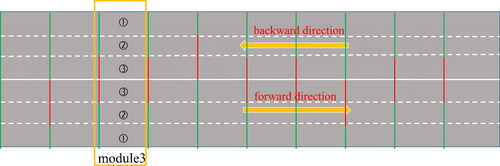
In the scenario of interest, we divided the roadway into 10 equal-length modules, with each module containing twice the maximum number of lanes. The signal lights were set as the boundaries between the modules. For example, in a case with four lanes, the maximum number of lanes in each direction is three (at least one lane needs to be open for each direction). As such, we would model a total of six lanes with three in each direction in VISSIM, as shown in Figure 3. The number of lanes is sorted from outside to inside, respectively from the first lane to the third lane. Each lane in the module has its corresponding signal head. A red light indicates that the lane is closed in the corresponding module, and a green light indicates that the lane is open. Then, according to the DLR scheme, we set different signal groups to control which lanes vehicles could pass through to realize the flexible number of lanes, i.e., 1-3, 2-2, and 3-1 configurations. The total number of red lights for each module should be exactly 2 in this case.

Figure 3. Proxy model of DLR in VISSIM.

The proposed VISSIM model adopts the calibrated parameters based on human drivers’ behaviors collected in Naturalistic Driving Study in Shanghai (Song & Sun, 2016; Sun et al., 2013). The specific parameter values are shown in Table 2.

Table 2. Default and recommended values of sensitive parameters.

	Parameter	Meaning	Default	Calibrated
Car following model	CC0	Average standstill distance (m)	1.5	2.1
	CC1	Headway time (s)	0.9	1.7
	CC2	Following variation (m)	4	3.2
	CC4&CC5	Negative and positive “following” threshold	−0.35	−0.35
Lane-changing model	MinD	Accepted deceleration of trailing vehicle(m/${\mathrm{s}}^2$)	−0.5	−1
	S_Fact	Safety distance reduction factor	0.6	0.35
	MaxCD	Maximum deceleration for cooperative breaking (m/${\mathrm{s}}^2$)	−3	−4.2
	MaxSD	Maximum speed difference (km/h)	10.8	16
	LC_Dist	Distance of lane-change attempt (m)	200	200

Numerical experiment

In both the CTM and VISSIM, the length of the road segment was set as 1 km, and the free-flow speed was set to 60 km/h. The time horizon was set as T = 600 s. Due to the obvious reduction in headway distance and an increase in traffic capacity with automatic vehicles, the capacity was set as 2000 pcu/h/ln. To ensure the passage of all vehicles, at least one lane was guaranteed for each direction. We made the following assumptions for the CTM specifically:

1. The DLR strategy of interest can operate at frequencies as high as 1/6 Hz, so the simulation interval length for CTM was set to 6 s, and the length for each module was set as 100 m. A total of 10 modules were populated. The lane direction update interval is 30 s. The backward wave speed was obtained from the q-k relationship diagram in the CTM model.

2. ${\mathrm{L}}_{\mathrm{a}}=2,{\mathrm{L}}_{\mathrm{b}}=2.$ Since the lane direction update interval is 30 s, the vehicles have enough time to change lanes twice to reorganize the fleet. In addition, lane changing by three lanes or more can seriously affect the safety of the vehicles on the road. For example, in a five-lane segment, the number of lanes cannot change from five to one or vice versa. As such, these extreme lane direction shifts were prohibited.

In the VISSIM simulation, some dedicated assumptions were made. The expected speed of vehicles was also set as 60 km/h. The flow in both directions was input to the road at the same time. The cycle time of the signal light is 30 s.

According to the characteristics of the DLR scheme and the actual traffic scenario, we made assumptions regarding the parameters of the NSGA-II algorithm as well. The relevant parameters are shown in Table 3.

Table 3. Parameters in the NSGA-II algorithm.

Number of Lanes	3	4	5	6	7	8
Parameters
Population Size	50	50	100	100	150	150
Evolutionary Algebra	200	200	300	300	400	400
Distribution Index for Crossover	20	20	20	20	20	20
Distribution Index for Mutation	20	20	20	20	20	20
Mutation Probability	0.05	0.05	0.05	0.05	0.05	0.05
Upper Bound of Lanes	2	3	4	5	6	7
Lower Bound of Lanes	1	1	1	1	1	1

Results and discussion

Pareto optimal solution

The Pareto frontier of the DLR scheme was obtained using the NSGA-II algorithm. Figure 4 shows the Pareto optimal solution of the DLR scheme with different lane conditions shown as Table 4. For Figure 4, the abscissa denotes the average vehicle delay and the ordinate denotes the corresponding driving safety hazard index.

Figure 4. Pareto-optimal solutions in various cases.

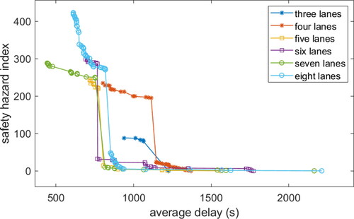
Table 4. Direction inflow rate for different lane conditions.

Parameters	Value
Number of Lanes	3	4	5	6	7	8
Directional Inflow Rate (pcu/h)	4500-4500	6000-6000	7500-7500	9000-9000	10500-10500	12000-12000

As one can see from Figure 4, the Pareto optimal solutions can be grouped into two separated regions. The first aggregation region occurred when the average delay was relatively high, while the driving safety hazard index was lower than 20. In this region, the Pareto optimal solutions are those with relatively fixed lane directions.

The second aggregation region forms when the average delay is lower than 200 seconds, while the driving safety hazard index is higher than 100. In this region, the optimal schemes are those with frequent lane direction changes.

Verification using VISSIM

We used the Component object model (COM) of VISSIM (Siddharth & Ramadurai, 2013) for tailor-made software development. Two DLR schemes with three lanes and six lanes were selected for validation purposes.

We implemented two optimal DLR schemes derived from the CTM in VISSIM. These two schemes were: 1) a three lane DLR scheme with a directional inflow rate of 900 pcu/h-900 pcu/h. and 2) a six lane DLR scheme with a directional inflow rate of 2400 pcu/h −2400 pcu/h. Since there were multiple optimal solutions along the Pareto frontier generated by NSGA-II, we implemented the solutions with the minimum average delay in VISSIM. In order to reduce the experimental error, ten repeated experiments were carried out and the average was taken. The corresponding results in terms of delays are shown in Figure 5.

Figure 5. Comparison of delays obtained in VISSIM and CTM.

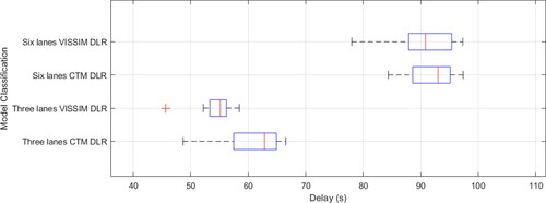
One can tell from Figure 5 that the delay results due to DLR obtained by the proxy model in VISSIM were like those derived by the CTM, which cross-validates the accuracy of the CTM.

During the experiment, it was found that the delay obtained by the proxy VISSIM model is quite sensitive to the distribution of desired speeds of vehicles. With a diversified desired speed distribution, it’s more likely that the delay result obtained by VISSIM stays close to or be even higher than that obtained by CTM. While with a unified desired speed distribution, the obtained delay result is relatively lower than that obtained by CTM. That said, with the current calibrated distribution of desired speed, the queuing delay obtained by VISSIM can fit with CTM, while if the distribution alters, discrepancy between VISSIM and CTM occurs.

Regression analysis

In this section, we discuss the relationships between different roadway features with respect to potential delay improvements due to DLR in order to shed light on DLR implementation priority. Note that minimizing the delay is the sole objective considered in this section. In previous studies, it was found that many key independent variables (length of the road segments, ratio of bidirectional traffic, total flow in both directions, number of lanes, etc.) have an impact on delay improvement. However, we found that the length of the segment did not have a significant impact on delay improvements due to DLR. As such, we focus on the influence of the remaining three independent variables on the resulting average vehicle delay improvement in this section.

By using SPSS for regression analysis, the bidirectional flow was summed to obtain the total flow tq, and the ratio of the bidirectional flow was converted into the variable proportion. Using the delay improvement value delay improve obtained by the CTM and NSGA-II as the dependent variable and tq, proportion, and the total number of lanes nlane as independent variables, we established a linear regression model. We also tested multiple regression models, including multiple logistic regression models, and found out that the linear one was optimal for this analysis.

The results of the linear regression model are shown in Table 5 below, and a regression result equation was obtained as well. (19) $$\mathrm{delayimprove}=-72.842+0.124\mathrm{t}\mathrm{q}-0.055\mathrm{proportion}+24.927\mathrm{nlane}$$(19)

Table 5. Result of regression parameter estimates.

Parameters	B	St.D. Error	P-Value	VIF
Nalne	24.927	.574	<.001	1.838
Tq	0.124	.001	<.001	1.897
Proportion	-.055	.072	<.001	1.054
(Constant)	−72.842	2.615
Model Fit	R Squared	Adjusted R Squared	St. Error of the Estimate	Durbin-Watson
	.523	.700	21.1613	.713

Based on the regression result Eq. (19)(19) $$\mathrm{delayimprove}=-72.842+0.124\mathrm{t}\mathrm{q}-0.055\mathrm{proportion}+24.927\mathrm{nlane}$$(19) , one can see that DLR should be implemented on roads with more lanes and higher total flow from both directions. We also suggest that DLR should be implemented on roads with relatively small discrepancies between the bidirectional flows.

The value of$\mathrm{ }{\overline{\mathrm{R}}}^2$ in the regression results was 0.723, which indicates satisfactory fitness.

Analysis of delay improvement results

We obtained the delay improvements from the DLR when compared to an optimal fixed lane scheme for a variety of inflow rates and total lane numbers using the CTM. The discrepancies between the delays achieved by the fixed and DLR schemes were derived and regarded as the delay improvement created by DLR. Figure 6 shows the results of the delay improvement. The x-axis and y-axis represent the incoming flows in the forward and backward direction respectively, and the z-axis represents the delay improvement due to DLR.

Figure 6. Average vehicle delay reduction (s) vs. directional flow (pcu/h).

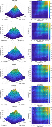
Since NSGA-II is heuristic, the optimal objective function value fluctuates, especially for cases with more total lanes. Such fluctuations could not be depicted explicitly. Therefore, we provide a discussion of the general patterns of the results. Our general observations are:

1. As the flow rate increased, the improvement in terms of delay generally increased as well. This is quite intuitive: vehicles are free to travel when the flow is low regardless of if DLR is implemented or not. Therefore, no noticeable improvement was observed. However, as the flow rate increased, DLR started to have more noticeable effects. If DLR was applied under these circumstances, the capacity in space and time could be fully utilized with respect to the dynamically changing occupancy within each module. This observation verifies that high frequency DLR is effective when applied to congested segments.

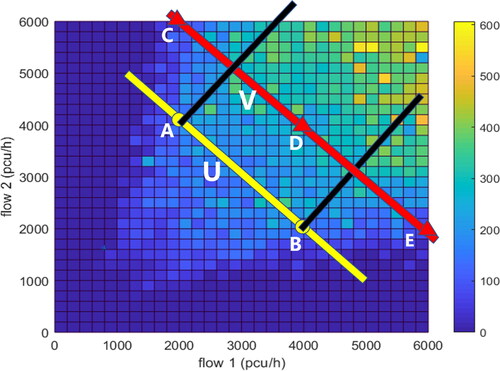
2. For segments with a total of n lanes, there existed n-2 critical protrusions (shown as points A and B in Figure 7) with delay reductions higher than the neighboring scenarios along their contour of the same amount of total inflow rates (shown as line U in Figure 7). In other words, there existed n-1 critical points (shown as triangular points C, D, and E in Figure 7) whose delay reduction was lower than neighboring scenarios along their contour (shown as line V in Figure 7). Using a four-lane case as an example, points C, D, and E correspond with the flow combinations that matched the capacity of each possible lane configuration (3-1, 2-2, and 1-3 lanes). Under such flow rate circumstances, it is ideal for the DLR to simply stay fixed at the corresponding lane configuration without any further dynamic changes despite the randomness of the flow rate. That being said, utilizing DLR did not significantly reduce delays. On the other hand, when the directional flow rate deviated from those three points, like at points A and B in Figure 7 the DLR shifted between the 3-1 and 2-2 lane configurations for point A and the 2-2 and 1-3 configurations for point B.

   Figure 7. Average vehicle delay reduction (s) vs. directional flow (pcu/h) in a situation with four lanes.

   

Analysis of driving safety hazard index

The variation in the driving safety hazard index when the minimum delay was achieved under different circumstances of bidirectional traffic flow is shown in Figure 8. Some observations include:

Figure 8. Driving safety hazard index vs. directional flow (pcu/h).

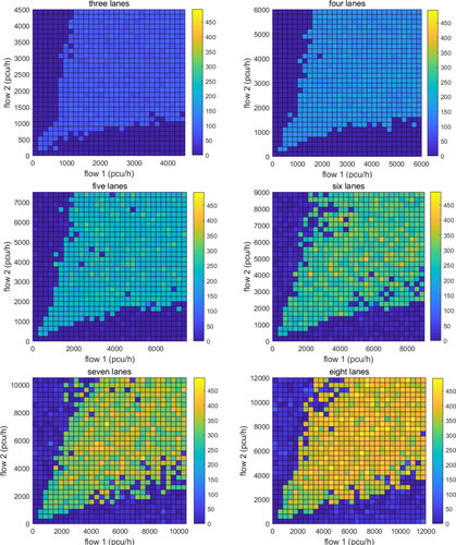
1. The maximum driving safety hazard index for all directional flow combinations increased with respect to the number of lanes. More lanes in general led to more possible configurations for the DLR lane directions, thus leading to more lane direction changes in order to achieve the lowest delay.

2. When the traffic flow in one direction was much higher than that in the other direction, the driving safety hazard index was extremely low with unnoticeable amounts of actual lane direction changes, such as when the bi-directional inflow rate was 10,500-1,750 pcu/h in the 7-lane case. The reason is that the effect of DLR is trivial with such a discrepancy in directional traffic flow as the road would essentially follow an extreme fixed lane scheme (e.g. 6-1 lane direction configuration in the 7-lane case). In this case, lane direction changes are infrequent, which leads to a lower safety hazard index. This simulation mechanism is intuitive and easy to implement.

3. The driving safety hazard index experiences a sudden change at the boundary between the low and high levels. The reason is that the number of lanes is always an integer in real life, so the decision variables must be integers as well when we solve the bi-objective programming problem. This leads to the discretized Pareto-optimal solutions.

Conclusion

In this paper we explored the possibility of adopting DLR to alleviate congestion and make full use of existing roadway capacity. When compared with traditional infrequent reversible lanes, DLR can adjusting lane directions in very short periods of time. The contributions of this paper are three-fold:

1. Using the CTM model, we considered the efficiency and safety of road driving to establish a bi-objective planning model. This paper used a NSGA-II algorithm to obtain a Pareto-optimal solution set and choose an optimal DLR scheme. This greatly reduced the complexity of our model construction and the influence of parameter settings.

2. A VISSIM-based DLR simulation model was developed. The simulation mostly focused on the delay differences before and after the implementation of DLR. The difficulty lay in the realization of dynamic reversible lanes in existing simulation environments. In this study, the COM interface was used for secondary development in VISSIM. By using a signal to control the lanes through which vehicles could pass through, we were able to alter the number of lanes in each direction.

3. We provide recommendations regarding the deployment of DLR in order to maximize delay reduction. First, DLR should be deployed in congested segments. Second, DLR should be prioritized for deployment on segments with more lanes. Third, DLR should be deployed on segments with directional flow that deviates far from exact capacity. However, tradeoffs between the safety hazard index and delay reduction were observed. Cases with higher delay reductions generally experienced higher safety hazard index.

This paper is the first step in studying the impact of DLR on congestion alleviation. There are additional modeling issues that should be explored further, including: (1) extending the model to provide the optimal location of DLR links within a network, (2) exploring the exact cause of the prediction off-set between VISSIM and CTM and establishing a more accurate VISSIM simulation model, (3) incorporating the equipment and setup cost of DLR in the optimization problem, and (4) calibrating and validation the proposed models using field-testing data of DLR.

Disclosure statement

No potential conflict of interest was reported by the author(s).

Additional information

Funding

This work was supported by the National Key Research and Development Program of China [2018YFB1600805], the Science and Technology Commission of Shanghai Municipality under Grant number [19DZ1208800], the National Natural Science Foundation of China under Grant number [52002279, 52172391], and the Shanghai Sailing Program under Grant number [19YF1451200].

References

- Agent, K. R., & Clark, J. D. (1982). Evaluation of reversible lanes. Traffic Engineering and Control, 23(11), 551–555.
- Ampountolas, K., & Carlson, R. C. (2019). Optimal control of motorway tidal flow [Paper presentation]. . 2019 18th European Control Conference (ECC), 25-28 June 2019. https://doi.org/10.23919/ECC.2019.8795879
- Ampountolas, k., Santos, J. A. d., & Carlson, R. C. (2020). Motorway tidal flow lane control. IEEE Transactions on Intelligent Transportation Systems, 21(4), 1687–1696. https://doi.org/10.1109/TITS.2019.2945910
- Bansal, P., & Kockelman, K. M. (2017). Forecasting Americans long-term adoption of connected and autonomous vehicle technologies. Transportation Research Part A: Policy and Practice, 95, 49–63. https://doi.org/10.1016/j.tra.2016.10.013
- Chu, K.-F., Lam, A. Y. S., & Li, V. O. K. (2020). Dynamic lane reversal routing and scheduling for connected and autonomous vehicles: Formulation and distributed algorithm. IEEE Transactions on Intelligent Transportation Systems, 21(6), 2557–2570. https://doi.org/10.1109/TITS.2019.2920674
- Claes, R., Holvoet, T., & Weyns, D. (2011). A decentralized approach for anticipatory vehicle routing using delegate multiagent systems. IEEE Transactions on Intelligent Transportation Systems, 12(2), 364–373. https://doi.org/10.1109/TITS.2011.2105867
- Daganzo, C. F. (1994). The cell transmission model: a dynamic representation of highway traffic consistent with the hydrodynamic theory. Transportation Research Part B: Methodological, 28(4), 269–287. https://doi.org/10.1016/0191-2615(94)90002-7
- Daganzo, C. F. (1995). The cell transmission model. II. Network traffic. Transportation Research Part B: Methodological, 29(2), 79–93. https://doi.org/10.1016/0191-2615(94)00022-R
- Deb, K. (2001). Multi-objective optimization using evolutionary algorithms (Vol. 16). John Wiley & Sons.
- Deb, K., & Agrawal, R. B. (1995). Simulated binary crossover for continuous search space. Complex Systems, 9(2), 115–148.
- Deb, K., & Agrawal, S. (1998). Understanding interactions among genetic algorithm parameters. In Foundations of genetic algorithms V. Morgan Kauffma.
- Deb, K., Pratap, A., Agarwal, S., & Meyarivan, T. (2002). A fast and elitist multiobjective genetic algorithm: NSGA-II. IEEE Transactions on Evolutionary Computation, 6(2), 182–197. https://doi.org/10.1109/4235.996017
- Dey, S., Ma, J., & Aden, Y. (2011). Reversible lane operation for arterial roadways: The Washington, D, USA experience. ITE Journal (Institute of Transportation Engineers), 81(5), 26–35.
- Gershenson, C., & Rosenblueth, D. A. (2012). Self-organizing traffic lights at multiple-street intersections. Complexity, 17(4), 23–39. https://doi.org/10.1002/cplx.20392
- Goel, S., Bush, S. F., & Gershenson, C. (2017). Self-organization in traffic lights: Evolution of signal control with advances in sensors and communications. arXiv preprint arXiv:1708.07188.
- Hausknecht, M., Au, T., Stone, P., Fajardo, D., & Waller, T. (2011). Dynamic lane reversal in traffic management [Paper presentation]. 2011 14th International IEEE Conference on Intelligent Transportation Systems. 14th International IEEE Conference on Intelligent Transportation Systems, 5-7 Oct. 2011, Piscataway, NJ, USA.
- Kim, S., & Shekhar, S. (2005, November). Contraflow network reconfiguration for evacuation planning: a summary of results [Paper presentation]. Proceedings of the 13th Annual ACM International Workshop on Geographic Information Systems.
- Levin, M. W., & Boyles, S. D. (2016). A cell transmission model for dynamic lane reversal with autonomous vehicles. Transportation Research Part C: Emerging Technologies, 68, 126–143. https://doi.org/10.1016/j.trc.2016.03.007
- Liu, P., Wu, J. M., Zhou, H. G., Bao, J., & Yang, Z. (2019). Estimating queue length for contraflow left-turn lane design at signalized Intersections. Journal of Transportation Engineering, Part A: Systems, 145(6), 04019020. https://doi.org/10.1061/JTEPBS.0000240
- Sangho, K., Shekhar, S., & Min, M. (2008). Contraflow transportation network reconfiguration for evacuation route planning. IEEE Transactions on Knowledge and Data Engineering, 20(8), 1115–1129. https://doi.org/10.1109/TKDE.2007.190722
- Siddharth, S. M. P., & Ramadurai, G. (2013). Calibration of VISSIM for Indian Heterogeneous traffic conditions. In P. Chakroborty, H. K. Reddy, A. Amekudzi, A. Das, A. Seyfried, B. Maitra, D. Teodorovic, K. K. Srinivasan, L. Devi, S. S. Pulugurtha, & T. V. Mathew (Eds.). 2nd Conference of Transportation Research Group of India (Vol. 104, pp. 380–389). https://doi.org/10.1016/j.sbspro.2013.11.131
- Song, R., & Sun, J. (2016). Calibration of a micro-traffic simulation model with respect to the spatial-temporal evolution of expressway on-ramp bottlenecks. Simulation, 92(6), 535–546. https://doi.org/10.1177/0037549716645197
- Sun, D., Zhang, L., & Chen, F. (2013). Comparative study on simulation performances of CORSIM and VISSIM for urban street network. Simulation Modelling Practice and Theory, 37, 18–29. https://doi.org/10.1016/j.simpat.2013.05.007
- Tian, Y., & Chiu, Y. C. (2014). A variable time-discretization strategies-based, time-dependent shortest path algorithm for dynamic traffic assignment. Journal of Intelligent Transportation Systems, 18(4), 339–351. https://doi.org/10.1080/15472450.2013.806753
- Xie, Y. C., Zhang, H. X., Gartner, N. H., & Arsava, T. (2017). Collaborative merging strategy for freeway ramp operations in a connected and autonomous vehicles environment. Journal of Intelligent Transportation Systems, 21(2), 136–147. https://doi.org/10.1080/15472450.2016.1248288
- Zheng, J., Liu, Y., & Sun, J. (2018). Research on influencing factors of traffic capacity in diverging area at urban expressway based on multilevel model. Traffic & Transportation, 01, 72–77.
- Zhou, W. W., Livolsi, P., Miska, E., Zhang, H., Wu, J., & Yang, D. (1993). An intelligent traffic responsive contraflow lane control system. In Proceedings of VNIS'93-Vehicle Navigation and Information Systems Conference.