An analysis of the value of optimal routing and signal timing control strategy with connected autonomous vehicles

Abstract

With the emergence of connected and automated technologies, Connected Autonomous Vehicles (CAVs) are able to communicate and interact with other vehicles and signal controllers. Vehicle to Vehicle (V2V) and Vehicle to Infrastructure (V2I) communications open up an opportunity to improve routing and signal timing efficiency with additional information from CAVs, such as prior travel time and signal green time. Most of the existing research on routing and signal timing for Human Driven Vehicles (HDVs) has to face the fact that human drivers only have partial knowledge about travel costs and traffic status on the road network, which typically reduces the system efficiency. In this paper, the impacts of additional information from CAVs on routing and signal timing efficiency in terms of total travel time have been investigated. An Optimal Routing and Signal Timing (ORST) control strategy for CAVs has been proposed and compared with four existing routing and signal timing strategies where drivers have different levels of information. The results of the simulation demonstrate that with additional information from CAVs, ORST can reduce about 49% of the total travel time compared with Stochastic User Equilibrium (SUE) and about 10% of the total travel time compared with User Equilibrium (UE).

KEYWORDS:

• Connected Autonomous Vehicles
• information
• routing
• signal timing
• system efficiency

1. Introduction

Efficiently assigning traffic flow and green time on a road network to reduce total travel time is a challenge to both drivers (including Human Driven Vehicles (HDVs) and Connected Autonomous Vehicles (CAVs)) and traffic managers. For an individual traveler, the shortest route, influenced by the route length, traffic flow and green time, should be identified to reduce individual travel time. For traffic managers, signal timing should be designed to reduce delay at junctions based on the demand at different phases.

Ideally, when drivers have full knowledge of the travel cost and traffic status on a road network, Wardrop’s first equilibrium, also known as User Equilibrium (UE), will be reached (Wardrop, 1952). However, in practice, it is not easy for all drivers to obtain full information about the network, which leads to the extension of Wardrop’s first equilibrium by scholars. For example, Daganzo and Sheffi (1977) proposed a revised behavioral principle that “no driver believes he can improve his travel time by unilaterally changing routes.” This principle allows drivers to have different levels of information about travel conditions, leading to the development of the Stochastic User Equilibrium (SUE) (Dial, 1971; Fisk, 1980).

Smith (1979a) proposed another version of the revised Wardrop’s first equilibrium “Consider a single driver who has travelled at least once today. He may use the same routes tomorrow. However, if he does change a route then he must change to a route which today was cheaper than the one he actually used today.” The revised principle proposed by Smith (1984) makes routing become a day-to-day re-routing process, where drivers can accumulate knowledge about the network by day-to-day re-routing and will reach equilibrium eventually.

Both of these extensions demonstrated that, in practice, human drivers do not have full knowledge of traffic conditions and their routing behaviors change corresponding to the different levels of information. With the emergence of connected and automated technologies, additional information such as vehicle trajectory (Cheng et al., 2022; Hu & Sun, 2019; Wang et al., 2020), mixed traffic conditions (Li et al., 2020; Olia et al., 2018) and signal timing (Mirheli et al., 2018) can be collected by sensors (So et al., 2022) on CAVs, which provides an opportunity for CAVs and signal controllers to reduce total travel time cooperatively. This leads to Wardrop’s second equilibrium (WP2), known as system optimal equilibrium, which states that average travel costs are minimized when all users behave cooperatively in routing (Wardrop, 1952).

Against this background, the main aim of this paper is to investigate the impacts of driver information levels on travel efficiency, which has been classified into three categories, namely network information, flow information and signal timing information, and propose a novel routing and signal timing control strategy to reduce total travel time when additional information from CAVs become available. The contributions of this paper are highlighted as follows:

1. The impacts of information levels on routing and signal timing efficiency have been investigated quantitatively. The results demonstrate that different levels of information will lead the road traffic system to different equilibrium points.

2. An Optimal Routing and Signal Timing (ORST) control strategy for CAVs has been proposed. Compared with existing routing and signal timing strategies, the ORST can further reduce the total time to achieve Wardrop’s second equilibrium with additional information from CAVs.

3. The sensitivity analysis of ORST under different demands and CAVs penetration rates demonstrates that when only part of the vehicles can behave cooperatively, system efficiency can still be improved with ORST, and the improvement is more significant at a high penetration rate and a mild congestion level.

The rest of this paper is organized as follows. In Sec. 2, literature related to routing and signal timing for HDVs and CAVs are reviewed. In Sec. 3, the levels of driver information of traffic conditions are discussed. Then four existing routing and signal timing strategies under different levels of driver information are introduced, and an Optimal Routing and Signal Timing (ORST) control strategy for CAVs is proposed. In Sec. 4, five routing and signal timing strategies under different levels of driver information are compared in a symmetrical network with Simulation of Urban Mobility (SUMO) (Lopez et al., 2018). In Sec. 5, we present a sensitivity analysis that takes mixed traffic conditions under different levels of demand into account. Section 6 concludes this paper.

2. Literature review

As routing and signal timing interact with each other, the opportunities to combine route choice and signal control have been explored by many researchers. Allsop (1974) discussed the possibilities of using traffic control to influence the route choice to achieve different UE. A few years later, Allsop and Charlesworth (1977) developed an iterative procedure where the TRANSYT software was used to calculate signal setting and estimate the relationship between link travel time and traffic flow. With the iterations of routing and signal setting, two different combinations of signal setting and traffic assignment were derived from the same OD matrix, which demonstrated that it is possible to influence route choice by signal setting.

Based on this idea of using traffic control to influence route choice, Smith (1979b) developed a theoretical model for the combined route choice and signal control problem. In this research, a simple network with two routes and a signal-controlled junction was used to demonstrate that the Webster (1958) method of signal setting did not maximize network capacity, because both Webster (1958) and TRANSYT (Robertson, 1969) ignored the influence of signal setting on route-choice. To maximize network capacity, Smith (1979b) proposed the P0 policy where saturated flow multiplying delay on one route should equal to another route. However, it should be noted that Smith assumed the travel time on both routes was the same. In other words, travel time on the route is not influenced by the flow on the link, which is unreasonable to some extent, because the total travel time on the network may not be minimized when the influence of flow on travel time is ignored.

Later, Smith (1981) extended the theoretical model to demonstrate that if the junction cost-flow function is continuous and the function tends to positive infinity when flow tends to link capacity, the problem of route choice and traffic signal control will have an equilibrium. However, Smith (1981) also pointed out that this condition might not be satisfied in practice and the practical implications for realistic networks need further study. Heydecker (1983) also found if the cost function increases strictly monotonically with the flow on the link, the equilibrium will have a unique solution. At a T-junction or signal-controlled junction, however, this condition is not always satisfied.

Taale and van Zuylen (2001) reviewed research on the combined route choice and signal control problem. They found that the iterative approach (Cantarella et al., 1991; Meneguzzer, 1995; Smith & Ghali, 1990), the global optimization approach (Chiou, 1999; Maher et al., 2001; Yang & Yagar, 1994) and the game-theoretic approach (Chen, 1998) are three main approaches that have been proposed to solve the combined route choice and signal control problem.

Recently, Smith (2015) extended his early theoretical research and formulated a theoretical dynamic system. Three dynamic relationships, including the relationship between route choice & route costs, route costs & bottleneck delay, and costs-bottleneck delay & green-time have been described mathematically. Then this triple dynamic relationship can be combined into a Lyapunov function for the whole system, which is guaranteed to converge to a convex set of equilibria with suitable variable step lengths.

With the emergence of connected technologies and autonomous vehicles, many researchers have started to pay attention to the interaction between CAVs and traffic signals. Guo et al. (2019) reviewed CAV based urban traffic control and roughly categorize existing studies into six categories, including driver guidance, actuated (adaptive) signal control, platoon-based signal control, planning-based signal control, signal-vehicle coupled control. They point out that CAV data have the potential to be used to estimate traffic states and make better signal timing plans.

Chai et al. (2017) investigated traveler’s route choice as affected by traffic signal control strategies. A VANET (Vehicular Ad hoc NETwork) was considered for route choice, where travelers have access to the real-time traffic information through V2V/V2I and make route choice decisions at each intersection using hyper-path trees. Six different traffic control strategies and three routing methods were simulated in OmNet++ and SUMO. The results showed that the proposed dynamic routing method can reduce overall travel cost and the proposed adaptive signal control reduces the average delay effectively.

Yu et al. (2018) proposed an integrated optimization model of traffic signal and vehicle trajectories at an isolated junction and found that ${CO}_2$ emssion and delay can be reduced. However, for simplicity, Newell’s car following model is used to modeling CAVs where vehicles are homogeneous and driving at the same desired speed.

Similarly, Xu et al. (2019) proposed a cooperative method to optimize the traffic signal timing and vehicle’s speed trajectories. The method is divided into two levels, including roadside traffic signal optimization and onboard vehicle speed control. As the proposed model is not a standard nonlinear programming problem, the enumeration method and the pseudospectral method are applied to solve the optimization problem and found that the proposed methods can improve transportation efficiency and fuel economy.

Both Yu et al. (2018) and Xu et al. (2019) assumed that all the vehicles in the system are CAVs. Recently, Tajalli and Hajbabaie (2022) proposed a cooperative signal timing and trajectory optimization with a mix of CAVs and Human-Drivern Vehicles (HDVs). The near-optimal solutions found 13% to 41% reduction in average travel time and 1% to 31% reduction in fuel consumption under different scenarios.

In summary, elaborate models for the combined route choice and signal control problem have been proposed in the last 45 years. Most of these models are designed for HDVs and have to face the fact that human drivers only have partial knowledge about travel costs and traffic status on the road network. With the emergence of connected and automated technologies, scholars are beginning to pay attention to the interaction between CAVs and traffic signals. However, most of the studies are focused on the cooperative optimization of vehicle trajectory and signal timing. The optimization of routing and signal timing is not fully studied. Though Chai et al. (2017) investigated traveler’s route choice as affected by traffic signal control strategies, the link travel time for the hyper-path trees is estimated by probabilities and the impacts of driver information levels on travel efficiency with different routing and signal timing strategies have not been taken into account. In the next section, the levels of information about traffic conditions and their improvement with CAVs will be discussed. Then, an ORST control strategy for CAVs will be proposed and compared with four widely-used routing and signal timing strategies under different levels of information.

3. Routing and signal timing strategies under different levels of information

3.1. Notations

Some notations used in this paper are listed in Table 1.

Table 1. Notations used in this paper.

Notations	Definitions
$G(N,L)$	A network including $N$ nodes, and $L$links
$\mathit{\text{od}}$	Index of OD
$a$	Index of link
$p$	Index of route
$n$	Index of node
$s$	Index of signal phases
$v_a$	Flow on link a
$C_a(\mathit{v},\mathit{\psi })$	Travel cost on link a
$n^{(\mathrm{s})}$	Nodes $n$ controlled by a signal with has$s$ phases
${\psi }_a^{n^{\left(s\right)}}({\gamma }_a^{n^{\left(s\right)}},{\mathit{\lambda }}_a^{n^{\left(s\right)}})$	Signal setting of s^th phase at signal-controlled nodes $n$ for link a
$\gamma$	Cycle time
$\mathit{\lambda }$	Durations of green as proportions of cycle time
$T_a(\mathit{v})$	Travel time on link a, when is not controlled by signal
$D_a^{\left(s\right)}(\mathit{v},{\psi }_a^{n^{(s)}}({\gamma }_a^{n^{(s)}},{\mathit{\lambda }}_a^{n^{(s)}}))$	Delay on link a
$Q_a$	Saturation flow on link a

3.2. The levels of information about traffic conditions

For an individual traveler, identifying the shortest route from the origin to the destination can significantly reduce individual travel time. To find the shortest route, travelers should have knowledge about the link travel cost $C_a(\mathit{v},\mathit{\psi }),$ which is related to the link $a,$ link flow $\mathit{v}$ and signal setting $\mathit{\psi }$ (Bifulco et al., 2016; Chiou, 2003; Yang & Yagar, 1995). Against this, the information about traffic conditions can also be divided into three categories.

The first category is information about the network, which is a fundamental level of information. For a network $G(N,L)$ with $N$ nodes and $L$links, drivers should have information about the network topological structure. Apart from the topological structure, the length of the link and the numbers of lanes are also important for drivers to estimate travel costs, which can be accessed from the map in some cities.

The second category is information about traffic flow $\mathit{v},$ which is an important level of information about traffic conditions. Based on the speed-flow-density relationship, drivers need to know the existing flow on the links to estimate link travel costs. However, in practice, human drivers only have partial knowledge about link flow, which can be acquired from their daily driving experience or navigation system, such as Advanced Traveler Information Systems (ATIS) (Bifulco et al., 2016). Without the help of sensors on CAVs and V2X communication technologies, it is hard for drivers to know accurate information about link flow.

The third category is information about the signal setting. As the delay at a signal-controlled junction $D_a^{\left(s\right)}(\mathit{v},\mathit{\psi })$ can be adjusted by green time $\mathit{\lambda }$ and cycle time $\gamma ,$ the signal setting is another information required for drivers to estimate link travel cost. However, in practice, human drivers only have limited knowledge about the signal setting at junctions, which also leads to the fact that the signal setting has been ignored by some routing strategies.

In summary, the levels of information about traffic conditions can be divided into three categories. Based on the different levels of information, different routing and signal timing strategies have been proposed by existing literature. The emergence of connected and automated technologies also provides an opportunity to get additional information from CAVs, such as accurate link flow and signal timing. In the next section, four existing routing and signal timing strategies under different levels of information will be introduced. Then an optimal routing and signal timing control strategy for CAVs will be proposed.

3.3. Existing routing and signal timing strategies

3.3.1. Shortest route and dijkstra’s algorithm

The most intuitive routing strategy for HDVs is to identify the shortest route based on the topological structure when the information about traffic flow and signal timing is not available or not reliable. To find the shortest route, Dijkstra’s algorithm (Dijkstra, 1959) has been developed to seek the shortest route between nodes in a network. However, in Dijkstra’s algorithm, the travel cost between nodes is a fixed value, which means the impacts of traffic flow and signal timing on travel cost have been ignored.

3.3.2. Stochastic routing

To allow human drivers to have different levels of information about travel conditions, Daganzo and Sheffi (1977) proposed a revised behavior principle that “no driver believes he can improve his travel time by unilaterally changing routes.” This principle leads to the extension of the Beckmann’s formulation shown as Eq. (1)(1) $$\underset{\mathit{v},\mathit{r}}{\mathrm{Minimize}}Z\left(\mathit{v}\right)={\sum }_{a\in L}\underset{v=0}{\overset{v_a}{\int }}{C}_a\left(v\right)dv$$(1) (Beckmann et al., 1956) to Eq. (2)(2) $$\begin{array}{c}\begin{array}{c}{r}_p>0\mathrm{ }\forall p\in P_{od}\\ {\sum }_{p\in P_{od}}{r}_p=R_{od}\end{array}\}\mathrm{ }\forall od\\ v_a=\sum _{od}\sum _{p\in P_{od}}{r}_p{\delta }_a^p\mathrm{ }\forall aϵ\mathit{\text{L}}\\ \underset{\mathit{v},\mathit{r}}{\text{Minimise}}Z\left(\mathit{v},\mathit{r}\right)=\sum _{a\in L}\underset{v=0}{\overset{v_a}{\int }}{C}_a\left(v\right)dv+\frac{1}{\theta }\sum _{od}\sum _{p\in P_{od}}{r}_p({\log }_e{r}_p-1)\end{array}$$(2) (Fisk, 1980). (1) $$\underset{\mathit{v},\mathit{r}}{\mathrm{Minimize}}Z\left(\mathit{v}\right)={\sum }_{a\in L}\underset{v=0}{\overset{v_a}{\int }}{C}_a\left(v\right)dv$$(1)

Subject to (2) $$\begin{array}{c}\begin{array}{c}{r}_p>0\mathrm{ }\forall p\in P_{od}\\ {\sum }_{p\in P_{od}}{r}_p=R_{od}\end{array}\}\mathrm{ }\forall od\\ v_a=\sum _{od}\sum _{p\in P_{od}}{r}_p{\delta }_a^p\mathrm{ }\forall aϵ\mathit{\text{L}}\\ \underset{\mathit{v},\mathit{r}}{\text{Minimise}}Z\left(\mathit{v},\mathit{r}\right)=\sum _{a\in L}\underset{v=0}{\overset{v_a}{\int }}{C}_a\left(v\right)dv+\frac{1}{\theta }\sum _{od}\sum _{p\in P_{od}}{r}_p({\log }_e{r}_p-1)\end{array}$$(2)

Subject to $$\begin{array}{c}\begin{array}{c}{r}_p>0\mathrm{ }\forall p\in P_{od}\\ {\sum }_{p\in P_{od}}{r}_p=R_{od}\end{array}\}\mathrm{ }\forall od\\ v_a=\sum _{od}\sum _{p\in P_{od}}{r}_p{\delta }_a^p\mathrm{ }\forall aϵ\mathit{\text{L}}\end{array}$$

The Lagrangian of Eq. (2)(2) $$\begin{array}{c}\begin{array}{c}{r}_p>0\mathrm{ }\forall p\in P_{od}\\ {\sum }_{p\in P_{od}}{r}_p=R_{od}\end{array}\}\mathrm{ }\forall od\\ v_a=\sum _{od}\sum _{p\in P_{od}}{r}_p{\delta }_a^p\mathrm{ }\forall aϵ\mathit{\text{L}}\\ \underset{\mathit{v},\mathit{r}}{\text{Minimise}}Z\left(\mathit{v},\mathit{r}\right)=\sum _{a\in L}\underset{v=0}{\overset{v_a}{\int }}{C}_a\left(v\right)dv+\frac{1}{\theta }\sum _{od}\sum _{p\in P_{od}}{r}_p({\log }_e{r}_p-1)\end{array}$$(2) can be rearranged as Eq. (3)(3) $$r_p=\mathrm{ }\frac{e^{-\theta C_p}}{\sum _{p\in P_{od}}{e}^{-\theta C_q}}\mathrm{ }{R}_{od}\mathrm{ }\forall \mathrm{ }p\in P_{od}\mathrm{ }\forall od$$(3) to calculate assigned route flow (Dial, 1971; Fisk, 1980), which can satisfy the Logit mechanism to allow drivers to have different levels of information about traffic conditions such as travel time. (3) $$r_p=\mathrm{ }\frac{e^{-\theta C_p}}{\sum _{p\in P_{od}}{e}^{-\theta C_q}}\mathrm{ }{R}_{od}\mathrm{ }\forall \mathrm{ }p\in P_{od}\mathrm{ }\forall od$$(3)

3.3.3. Proportional-switch adjustment process (PAP)

As previously discussed in Sec. 1, though drivers might not have perfect information about traffic conditions, they can accumulate knowledge by day-to-day traveling. Smith (1979a) proposed that a driver might use the same routes tomorrow. However, if a driver changes the route, the new route must be a cheaper one. Based on this idea, He et al. (2010) proposed a Proportional-switch Adjustment Process (PAP), where travelers’ cost-minimisation behavior in their path findings and their inertia are captured by the day-to-day re-routing process.

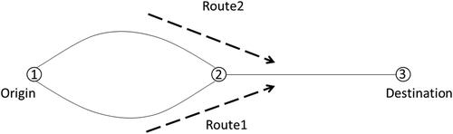
Taking a simple network as shown in Figure 1 for example, on a specific day $t,$ the travel cost via Route 1 $C_1(v_1(t))$ is lower than the travel cost using Route 2 $C_2(v_2(t)).$ Assuming drivers have information about historical travel time, a proportional of travelers will shift from Route 2 to Route 1 at day $t+1,$ which is an increasing function of Route 2 flow $v_2\left(t\right)$ and the difference in travel cost between two routes.

Figure 1. A simple network with two routes.

Therefore, the flow vector $\mathit{v}\left(\mathit{t}\right)=\left[v_1\right(t),\mathrm{ }{v}_2(t\left)\right];$ travel cost vector$\mathrm{ }\mathit{C}\left(\mathit{v}\left(\mathit{t}\right)\right)={[C}_1\left(\mathit{v}\left(t\right)\right),C_2\left(\mathit{v}\left(t\right)\right)]$ and the changes ${\Delta }_1\left(\mathit{v}\left(\mathit{t}\right)\right),{\Delta }_2\left(\mathit{v}\left(\mathit{t}\right)\right)$ satisfy Eqs. (4)(4) $${\Delta }_1\left(\mathit{v}\left(\mathit{t}\right)\right)=\mathrm{ }-w{v}_2\left(t\right)\left[C_2\left(\mathit{v}\left(t\right)\right)-C_1\left(\mathit{v}\left(t\right)\right)\right]$$(4) and (5)(5) $${\Delta }_2\left(\mathit{v}\left(\mathit{t}\right)\right)= w{v}_2\left(t\right)\left[C_2\left(\mathit{v}\left(t\right)\right)-C_1\left(\mathit{v}\left(t\right)\right)\right]$$(5) . (4) $${\Delta }_1\left(\mathit{v}\left(\mathit{t}\right)\right)=\mathrm{ }-w{v}_2\left(t\right)\left[C_2\left(\mathit{v}\left(t\right)\right)-C_1\left(\mathit{v}\left(t\right)\right)\right]$$(4) (5) $${\Delta }_2\left(\mathit{v}\left(\mathit{t}\right)\right)= w{v}_2\left(t\right)\left[C_2\left(\mathit{v}\left(t\right)\right)-C_1\left(\mathit{v}\left(t\right)\right)\right]$$(5)

Smith (2015) further extended the PAP process to a general road network as Eq. (6)(6) $${\Delta }_{\mathit{ODq}}\left(\mathit{v}\right)=\sum _{\left(r,s\right):r<s}\mathrm{ }w\left\{v_{qr}\right[C_{qr}\left(\mathit{v}\left(t\right)\right)-C_{qs}\left(\mathit{v}\left(t\right)\right){]}_{+}{\Delta }_{\mathit{qrs}}+v_{qs}\left[C_{qs}\right(\mathit{v}\left(t\right))-C_{qr}(\mathit{v}\left(t\right)\left){]}_{+}{\Delta }_{\mathit{qrs}}\right\}\mathrm{ }$$(6) and demonstrated that it could be applied to a general network. (6) $${\Delta }_{\mathit{ODq}}\left(\mathit{v}\right)=\sum _{\left(r,s\right):r<s}\mathrm{ }w\left\{v_{qr}\right[C_{qr}\left(\mathit{v}\left(t\right)\right)-C_{qs}\left(\mathit{v}\left(t\right)\right){]}_{+}{\Delta }_{\mathit{qrs}}+v_{qs}\left[C_{qs}\right(\mathit{v}\left(t\right))-C_{qr}(\mathit{v}\left(t\right)\left){]}_{+}{\Delta }_{\mathit{qrs}}\right\}\mathrm{ }$$(6) where $x_{+}=\max \{x,0\};$ ${\Delta }_{\mathit{qrs}}$ is the swap vector from Route $r$ to Route $s$ for OD pair $q.$

3.3.4. PAP and P0 policy

To take signal timing into account, Smith (2015) further extended the proportional-switch adjustment process to embrace green time using the P0 policy. The policy moves green-time from less pressurized stages to more pressurized stages in which the pressures are measured by the bottleneck delay and saturated flow. For example, in the network of Figure 1 where Node 2 is a signal-controlled junction, the adjustment of green time will influence bottleneck delay on two routes. When the bottleneck delay $b_1$ multiplies the saturated flow $s_1$ on Route 1 higher than the one using Route 2, i.e. $s_1{b}_1>s_2{b}_2,$ green timing should be swapped from Route 2 to Route 1 to reduce delay at the junction. The change of green timing should satisfy Eqs. (7)(7) $${\Delta \mathrm{G}}_1\left(\mathit{t}\right)=\mathrm{ }w{G}_2\left(t\right)\left[s_1{b}_1\right(t)-s_2{b}_2(t){]}_{+}-w{G}_1(t\left)\right[s_2{b}_2\left(t\right)-s_1{b}_1\left(t\right){]}_{+}$$(7) and (8)(8) $${\Delta \mathrm{G}}_2\left(\mathit{t}\right)=\mathrm{ }-w{G}_2\left(t\right)\left[s_1{b}_1\left(t\right)-s_2{b}_2\left(t\right)\right]+w{G}_1\left(t\right)\left[s_2{b}_2\right(t)-s_1{b}_1(t){]}_{+}\mathrm{ }$$(8) . (7) $${\Delta \mathrm{G}}_1\left(\mathit{t}\right)=\mathrm{ }w{G}_2\left(t\right)\left[s_1{b}_1\right(t)-s_2{b}_2(t){]}_{+}-w{G}_1(t\left)\right[s_2{b}_2\left(t\right)-s_1{b}_1\left(t\right){]}_{+}$$(7) (8) $${\Delta \mathrm{G}}_2\left(\mathit{t}\right)=\mathrm{ }-w{G}_2\left(t\right)\left[s_1{b}_1\left(t\right)-s_2{b}_2\left(t\right)\right]+w{G}_1\left(t\right)\left[s_2{b}_2\right(t)-s_1{b}_1(t){]}_{+}\mathrm{ }$$(8) where $G_i\left(t\right)$is the green time on link $i;$ ${\Delta G}_i\left(\mathit{t}\right)$ is the change of green time for the next iteration on link $i;$ $s_i$ is the saturation flow at the exit of link $i;$ $b_i\left(t\right)$ is the bottleneck delay at the exit of link $i$ and $w$ is the weight of proportional-switch adjustment process. Based on the Lyapunov function, Smith proved that combining routing and signal timing dynamic system can converge to equilibrium.

3.4. Optimal routing and signal timing (ORST) control strategy

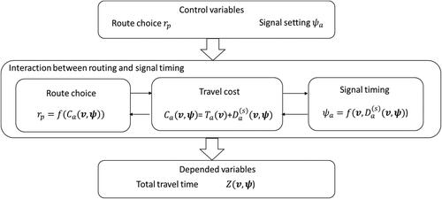
As CAVs are able to communicate and interact with other CAVs and signal controllers, the interaction between routing and signal timing can be summarized in Figure 2. For a road traffic system, the total travel time $Z\left(\mathit{v},\mathit{\psi }(\gamma ,\mathit{\lambda })\right)$ is a dependent variable controlled by the route choice $r_p$ and the signal setting ${\psi }_{\mathrm{a}}.$ Given the information about travel flow $v$ and signal setting $\mathit{\psi },$ the route choice $r_p$ is depended on the travel cost of the links $C_a(\mathit{v},\mathit{\psi }).$ Given the information about travel flow $\mathit{v}$ and junction delay $D_a(\mathit{v},\mathit{\psi }),$ the signal setting can be adjusted correspondingly.

Figure 2. The interaction between routing and signal timing.

At the microscopic level, CAV can route cooperatively with traffic signals to reduce total travel time, in other words, minimizing public cost as shown in Eq. (9)(9) $$e_p\left\{\begin{array}{c}>0\mathrm{ }\Rightarrow \mathrm{ }{C}_p+\sum _{\forall a}{\delta }_p^a{v}_a\frac{\partial c_a(v_a,\mathit{\psi })}{\partial v_a}=C_{od}^{\mathrm{*}}\\ =0\mathrm{ }\Rightarrow \mathrm{ }{C}_p+\sum _{\forall a}{\delta }_p^a{v}_a\frac{\partial c_a(v_a,\mathit{\psi })}{\partial v_a}\ge C_{od}^{\mathrm{*}}\end{array}\right\}\mathrm{ }\forall pϵP_{od},\mathrm{ }\forall od$$(9) . (9) $$e_p\left\{\begin{array}{c}>0\mathrm{ }\Rightarrow \mathrm{ }{C}_p+\sum _{\forall a}{\delta }_p^a{v}_a\frac{\partial c_a(v_a,\mathit{\psi })}{\partial v_a}=C_{od}^{\mathrm{*}}\\ =0\mathrm{ }\Rightarrow \mathrm{ }{C}_p+\sum _{\forall a}{\delta }_p^a{v}_a\frac{\partial c_a(v_a,\mathit{\psi })}{\partial v_a}\ge C_{od}^{\mathrm{*}}\end{array}\right\}\mathrm{ }\forall pϵP_{od},\mathrm{ }\forall od$$(9) As CAVs will routing cooperatively with traffic signals to minimize public cost, at the macroscopic level, total travel time should be minimized. Therefore, an optimization problem can be formulated as in Eq. (10)(10) $$\underset{v,t,\mathit{\psi }(\gamma ,\mathit{\lambda })}{\mathrm{Minimize}}Z\left(\mathit{v},\mathit{\psi }(\gamma ,\mathit{\lambda })\right)={\sum }_{a\in L}{v_a\mathrm{ }C}_a(\mathit{v},\mathit{\psi })={\sum }_{a\in L}{v_a[T}_a\left(\mathit{v}\right)+{{\delta }_a^{n^{\left(\mathrm{s}\right)}}D}_a^{n^{\left(s\right)}}(\mathit{v},\mathit{\psi })]$$(10) . (10) $$\underset{v,t,\mathit{\psi }(\gamma ,\mathit{\lambda })}{\mathrm{Minimize}}Z\left(\mathit{v},\mathit{\psi }(\gamma ,\mathit{\lambda })\right)={\sum }_{a\in L}{v_a\mathrm{ }C}_a(\mathit{v},\mathit{\psi })={\sum }_{a\in L}{v_a[T}_a\left(\mathit{v}\right)+{{\delta }_a^{n^{\left(\mathrm{s}\right)}}D}_a^{n^{\left(s\right)}}(\mathit{v},\mathit{\psi })]$$(10)

Subject to $$\begin{array}{c}\mathrm{ }\begin{array}{c}{r}_p>0\mathrm{ }\forall p\in P_{od}\\ {\sum }_{p\in P_{od}}{r}_p=R_{od}\end{array}\}\mathrm{ }\forall od\mathrm{ }\left(\mathit{Demand}\mathrm{ }\mathit{constraint}\right)\\ v_a=\sum _{od}\sum _{p\in P_{od}}{r}_p{\delta }_a^p\mathrm{ }\forall aϵ\mathit{\text{L}}\mathrm{ }\left(\text{Link}\mathrm{ }\text{flow}-\text{route}\mathrm{ }\text{flow}\mathrm{ }\text{constraint}\right)\\ \sum _{a\in L}\sum _{s\in S}{\lambda }_a^{n^{(s)}}{\delta }_a^{n^{(s)}}=1\mathrm{ }\forall nϵN^{\left(\mathit{S}\right)}\mathrm{ }(\text{signal}\mathrm{ }\text{timing}\mathrm{ }\text{constraint})\\ \mathrm{ }{\delta }_a^{n^{(\mathrm{s})}}=\{\begin{array}{c}1 if \mathit{link} a is \mathit{controlled} by s^{th} \mathit{phase} at \mathit{node} n \\ 0 \mathit{otherwise} \end{array}\\ \mathrm{ }{v}_a\le \mathrm{ }\sum _{s\in S}{\lambda }_a^{n^{(s)}}{Q}_a\mathrm{ }\left(\text{Link}\mathrm{ }\text{capacity}\mathrm{ }\text{constraint}\right)\end{array}$$The equation is derived from the System Optimal (SO) traffic assignment, where demand constraint,$\mathrm{ }$link flow-route flow constraint, signal timing constraint and capacity constraint should be satisfied. For any route $p,$ the flow on this route should be larger than zero and the sum of all routes from the origin to the destination should equal to demand of this OD pair. For any link $a,$ the flow on this link should equal to the sum of route flows, using this link; meanwhile, the link flow $a$ should not exceed the link capacity. For any signal-controlled nodes, the sum of proportional green time at different phases should equal to one.

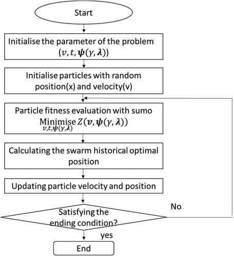
Considering the lack of real-world data at this stage to calibrate the link travel cost function $C_a(\mathit{v},\mathit{\psi })$ for CAVs, the $C_a(\mathit{v},\mathit{\psi }),$ including travel time and bottleneck delay, will be calculated by SUMO simulation, where CAVs are controlled by Cooperative Adaptive Cruising Control (CACC) (Milanés & Shladover, 2014). As the link travel cost function $C_a\left(\mathit{v},\mathit{\psi }\right)$ calculated by simulation is nonlinear, the Particle Swarm Optimization (PSO) approach proposed by Kennedy and Eberhart (1995) to solve nonlinear optimization problems, where particles are used to search for optimal solutions as a stylized representation of bird flocking or fish schooling movements, will be adopted and the flow chat of PSO are shown in Figure 3.

Figure 3. The flow chat of PSO.

3.5. Summary

To sum up, the levels of information about traffic conditions can be divided into three categories. Based on the different levels of information, four existing routing and signal timing strategies under different levels of information and a proposed ORST control strategy for CAVs have been summarized in Table 2. In the next section, these five routing and signal timing strategies will be compared in a symmetrical network with SUMO.

Table 2. The summary of routing and signal timing strategies under different levels of information.

Levels of information		Shortest route	Stochastic routing	PAP	PAP + P0	ORST
Network	Topological structure	√	√	√	√	√
	Link length	√	√	√	√	√
	Numbers of lanes	√	√	√	√	√
Flow	Partial knowledge		√
	Historical flow			√	√	√
	Actual flow					√
Signal timing	Green time				√	√

4. Case study of routing and signal timing strategies under different levels of information

4.1. Overview of the network structure and parameter setting

To investigate the impacts of information levels on routing and signal timing efficiency and whether travel efficiency can be improved with information from CAVs. Four existing routing and signal timing strategies under different levels of information and a proposed ORST control strategy for CAVs will be compared in the network $G(N=5,L=6)$ shown as Figure 4.

Figure 4. The structure of a road network.

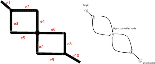
The network $G(N=5,L=6)$ has five nodes, including a signal-controlled node (Node 3) and six links. The length of each edges shown in Figure 4 is 500 meters with two lanes. The yellow time between phases is set as 3 s, and the initial green time for edge 4 and edge 5 are 30 s and 70 s. The cycle time of the junction is set as 106 s. Travel demand is 2000 vehicle/h from the origin point to the destination point and four available routes can be identified as follow:

• Route 1 (Main) = edge_1 edge_2 edge_4 edge_7 edge_9 edge_10

• Route 2 (Main) = edge_1 edge_3 edge_5 edge_6 edge_8 edge_10

• Route 3 = edge_1 edge_2 edge_4 edge_6 edge_8 edge_10

• Route 4 = edge_1 edge_3 edge_5 edge_7 edge_9 edge_10

Based on the vehicle following model reviewed by Li et al. (2020), Krauss model is used to model the following behavior of HDVs, and CACC controller is used to model the following behavior of CAVs. The parameters are shown in Table 3.

Table 3. Parameters for SUMO simulation.

Krauss model for HDVs simulation	CACC controller for AVs simulation
$a_{\max }=2.6 m/s^2$	$a_{\max }=2.6 m/s^2$
$b=4.0 m/s^2$	$b=5.0 m/s^2$
$\tau =1.5 s$	$t_{sw}=1 s$
$\sigma =0.5$	$\sigma =0$
	$k_p=0.45$
	$k_d=0.25$

A laptop with Intel(R) Core(TM) i7-8750H CPU @ 2.20 GHz, 2208 Mhz, 6 Core(s), 12 Logical Processor(s), 32.0 GB RAM and NVIDIA GeForce GTX 1060 is used as the computation platform. The computation time of each simulation (for example a iteration of PAP or a Particle in an iteration of PSO) is from 60 s to 120 s.

4.2. Routing and signal timing under different levels of information

4.2.1. Strategy 1: Shortest route

As discussed in Sec. 3, when the information about traffic flow and the signal timing is not available or not reliable, identifying the shortest route based on the topological structure is a reasonable strategy for drivers to minimize total travel time. The MAROUTER, which uses a hard-coded capacity-constraint function based on the speed limit, lane number and edge priority to compute travel time in SUMO, has been applied to estimate travel cost.

As the network is symmetrical, the travel cost on each route is the same when the information about signal timing is not available. MAROUTER assigns 1000 vehicles to Route 3 and another 1000 vehicles to Route 4. However, the actual green timing for these two routes is different, which means that the real travel time on Route 3 and Route 4 might also be different. Based on the results of the simulation, the actual average travel cost on Route 3 and Route 4 are 2009.1s and 569.6 s.

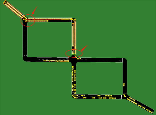
The results demonstrate that though drivers can identify the shortest route based on the topological structure when the information about traffic flow and the signal timing is not available or not reliable, it is not reasonable in some circumstances. Congestion might occur when the information about flow and signal timing has been ignored. As shown in Figure 5, unreasonable routings cause congestion on edge 4 and the shockwaves caused by congestion and queueing further affect vehicles at Node 2.

Figure 5. An example of shockwaves caused by congestion and queueing.

4.2.2. Strategy 2: Stochastic routing

In practice, not only do drivers have information about the network topological structure, but also they have some knowledge about traffic conditions based on their driving experience, which means a stochastic user equilibrium can be achieved under this circumstance. The DUAROUTER, based on Eq. (3)(3) $$r_p=\mathrm{ }\frac{e^{-\theta C_p}}{\sum _{p\in P_{od}}{e}^{-\theta C_q}}\mathrm{ }{R}_{od}\mathrm{ }\forall \mathrm{ }p\in P_{od}\mathrm{ }\forall od$$(3) for SUE, in SUMO has been applied for routing, where route cost $C_p$ is calculated from the last simulation and $\theta$ is scaled by the sum of all routes.

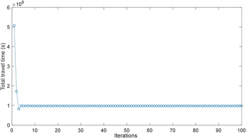
As shown in Figure 6, the system iteratively converges to an equilibrium point. Based on the results of the simulation, at the stochastic user equilibrium, 723 vehicles chose Route 2; 537 vehicles chose Route 3; 740 chose Route 4; the travel cost on each used route is 311 s, and the total travel time is 984,098 s.

Figure 6. Total travel time vs. iterations (SUE).

4.2.3. Strategy 3: PAP

As discussed in Sec. 1, though drivers might not have perfect information about traffic conditions, they can accumulate knowledge by day-to-day traveling. When drivers have information about yesterday’s travel time, based on the proportional-switch adjustment process, some vehicles might shift from a high-cost route to a low-cost route today.

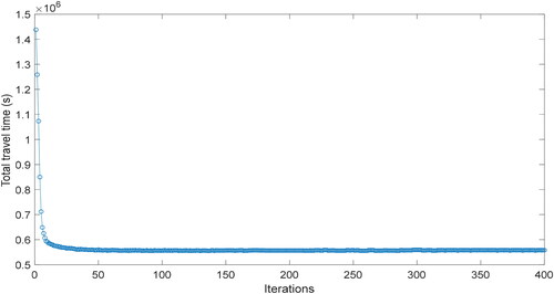
Considering the structure of the network, going straight does not need to reduce the speed for turning. Route 1 and Route 2 have been set as two main routes for the proportional-switch adjustment process and the results are shown in Figure 7, in which the PAP strategy makes the system converge to a different equilibrium point where total travel time is 558,041 s.

Figure 7. Total travel time vs. iterations (PAP).

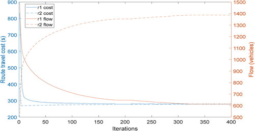
The changes in route flow and travel cost are shown in Figure 8. At the beginning stage, travel cost on Route 1 $C_1\left(\mathit{v}\left(t\right)\right)$ is higher than travel cost on Route 2 $C_2\left(\mathit{v}\left(t\right)\right).$ Though drivers do not have information about signal timing and current link flow, historical travel time helps them move to a user equilibrium point. When historical travel time on Route 1 $C_1\left(\mathit{v}\left(t\right)\right)$ is higher than historical travel time on Route 2 $C_2\left(\mathit{v}\left(t\right)\right),$ a part of the flow will shift from Route 1 to Route 2. Eventually, the system approaches an equilibrium state, where 613 vehicles choose Route 1 with 278.8 s average travel time and 1387 vehicles choose Route 2 with an average travel time of 279.1 s.

Figure 8. The changes of route flow and travel cost with PAP.

4.2.4. Strategy 4: PAP + P0

Though proportional-switch adjustment process leads to an equilibrium state, the influence of signal control on routing has been ignored. To take signal control into account, PAP has been combined with P0 policy in this scenario, which tries to reduce delay at the junction and maximize road capacity. When the bottleneck delay multiplied by saturated flow on Route 1 is higher than Route 2, i.e. $s_1{b}_1>s_2{b}_2,$ green timing will be swapped from Route 2 to Route 1.

According to the results of the simulation shown in Figures 9 and 10, the combined PAP and P0 policy makes the system converge to a new equilibrium point where total travel time is 552,985 s. To reduce junction delay, the green time on Route 1 increases from 30 s to 43 s; meanwhile, the green time on Route 2 decreases from 70 s to 57 s.

Figure 9. Total travel time vs. iterations (PAP + P0).

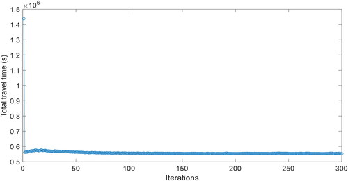
Figure 10. (a) Change of route flow and travel cost; (b) Change of green time and delay.

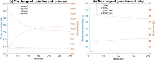
At the equilibrium point, where drivers cannot improve their travel time by unilaterally changing routes, 47.25% of the total flow choose Route 1 with 276.6 s average travel time and 4.8 s average delay, while 52.75% of the total flow choose Route 2 with 276.3 s average travel time and 4.7 s average delay.

4.2.5. Strategy 5: ORST

As discussed in Secs. 1 and 3, with the emergence of connected and automated technologies, CAVs provided an opportunity to improve travel efficiency with additional information from CAVs and signal controller. Considering that CAVs and signal controllers can interact with each other, an optimization problem can be formulated as shown in Eq. (10)(10) $$\underset{v,t,\mathit{\psi }(\gamma ,\mathit{\lambda })}{\mathrm{Minimize}}Z\left(\mathit{v},\mathit{\psi }(\gamma ,\mathit{\lambda })\right)={\sum }_{a\in L}{v_a\mathrm{ }C}_a(\mathit{v},\mathit{\psi })={\sum }_{a\in L}{v_a[T}_a\left(\mathit{v}\right)+{{\delta }_a^{n^{\left(\mathrm{s}\right)}}D}_a^{n^{\left(s\right)}}(\mathit{v},\mathit{\psi })]$$(10) . To solve this optimization problem, the Particle Swarm Optimization (PSO) has been adopted, because of the nonlinear feature of the link travel cost $C_a\left(\mathit{v},\mathit{\psi }\right)$ calculated by simulation.

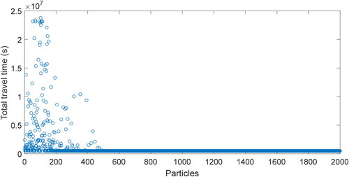
The population of the particles is pre-set as 40 and the results of 50 iteration runs is shown in Figure 11. A converged optimal solution has been calculated with the total travel time of 501,659 s. At the converged point, 1999 vehicles use Route 1 with 95 s green time and 250.8 s average travel time. Only 1 vehicle uses Route 2 with 5 s green time and 328 s average travel time.

Figure 11. Total travel time vs. particles (ORST).

4.3. Summary

In summary, the proposed ORST control strategy for CAVs has been compared against four existing routing and signal timing strategies under different levels of information to investigate the impacts of information levels on routing and signal timing efficiency. The results are summarized in Table 4 and Figure 12, which demonstrate that with additional information from CAVs, ORST can reduce approximately 49% of the total travel time compared with SUE and approximately 10% of the total travel time compared with UE.

Figure 12. Total travel time of routing and signal timing strategies under different levels of information.

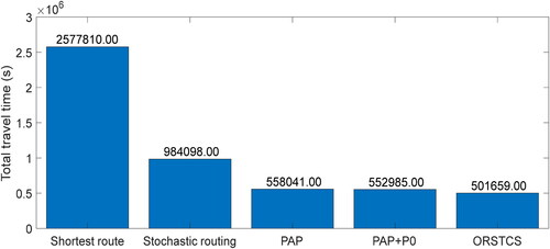
Table 4. Results of routing and signal timing strategies under different levels of information.

Strategies Results	Shortest route	Stochastic routing	PAP	PAP + P0	ORST
Route 1 flow (vehicle/h)	na	na	613	945	1999
Route 2 flow (vehicle/h)	na	723	1387	1055	1
Route 3 flow (vehicle/h)	1000	537	na	na	na
Route 4 flow (vehicle/h)	1000	740	na	na	na
Route 1 cost(s)	na	na	278.8	276.6	250.8
Route 2 cost(s)	na	311^a	279.1	276.3	328
Route 3 cost(s)	2009.1	311^a	na	na	na
Route 4 cost(s)	569.6	311^a	na	na	na
Edge 4 greentime (s)	30	30	30	43	95
Edge 5 greentime (s)	70	70	70	57	5
Total traveltime (s)	2,577,810	984,098	558,041	552,985	501,659

a Edge based travel time is estimated by the mean speed in SUMO.

The impacts of information levels on routing and signal timing efficiency can be concluded as follows. Firstly, comparing the shortest route strategy with stochastic routing or PAP strategies, partial information about traffic flow can help the road traffic system reach a stochastic user equilibrium or user equilibrium point, which can reduce congestion caused by unreasonable routing. Secondly, with information from signal timing, a better user equilibrium can be achieved with PAP + P0 policy to reduce total travel time by adjusting signal timing. Thirdly, when additional information from CAVs becomes available via V2V and V2X communications, ORST can make CAVs behave cooperatively to achieve WP2, where total travel time can be further reduced.

5. Sensitivity analysis of mixed traffic conditions

The case studies in Sec. 4 have demonstrated that total travel time can be significantly reduced with the proposed ORST control strategy in a pure CAV scenario. However, in practice, CAVs cannot replace HDVs to achieve a fully connected and automatic environment in the short term. Hence, this section will investigate whether travel efficiency can still be improved by the ORST control strategy in mixed traffic conditions of CAVs and HDVs.

The sensitivity analysis is conducted to evaluate the performance of the ORST control strategy under different CAV penetration rates and demands. The population of the PSO particles is pre-set as 40 and the results of total travel time of 50 iterations are shown in Figure 13(a)–(c). It can be observed from Table 5 and Figure 13(d) that when the demand is 2000 vehicle/h, the total travel time decreases with the increase of CAV penetration rate. As expected, the reduction is mild at a low penetration rate and more significant at a high penetration rate when more CAVs are able to cooperate with other vehicles and signals.

Figure 13. Sensitivity analysis for mixed CAV conditions.

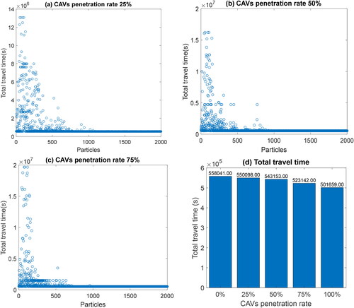
Table 5. The sensitivity analysis of ORTS under different CAVs penetration rates.

Penetration Results	0%	25%	50%	75%	100%
Route 1 HDVs flow (vehicle/h)	613	460	307	153	0
Route 2 HDVs flow (vehicle/h)	1387	1040	693	347	0
Route 1 CAVs flow (vehicle/h)	0	213	999	1494	1999
Route 2 CAVs flow (vehicle/h)	0	287	1	6	1
Route 1 cost (s)	278.8	282.0	260.6	285.9	250.8
Route 2 cost (s)	279.1	271.5	292.3	264.8	328.0
Edge 4 greentime (s)	30	28	67	81	95
Edge 5 greentime (s)	70	72	32	80	5
Total traveltime (s)	558,041	550,098	543,153	523,142	501,659

To further evaluate the performance of ORTS under different congestion levels, the demand varies from 1000 vehicle/h to 3000 vehicle/h. As shown in Table 6 and Figure 14, both the total and average travel time climb with increasing demand, which indicates that the system performance of a road network will drop with the increase of users in a congestion condition.

Figure 14. Total and average travel time under different demands and penetration rates.

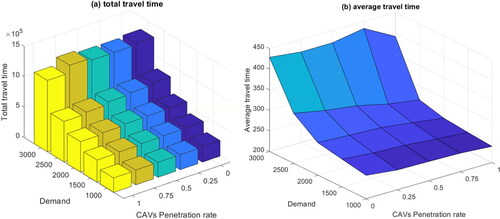
Table 6. The sensitivity analysis of ORTS under different demands and penetration rates.

Penetration Demand (veh/h)	Total travel time(s)					Average travel time(s)
	0%	25%	50%	75%	100%	0%	25%	50%	75%	100%
1000	256,835	248,197	246,895	245,025	239,314	256.8	248.2	246.9	245.0	239.3
1500	401,611	391,439	386,480	376,240	366,960	267.7	261.0	257.7	250.8	244.6
2000	558,041	550,098	543,153	523,142	501,659	279.0	275.0	271.6	261.6	250.8
2500	804,412	766,581	740,211	695,596	666,005	321.8	306.6	296.1	278.2	266.4
3000	1,286,706	1,259,283	1,260,353	1,298,728	1,175,031	428.9	419.8	420.1	432.9	391.7

In order to quantitatively evaluate the performance of ORTS under different demands, the reduction rate of the average travel time is shown in Figure 15, which illustrates that with ORTS control strategy, the improvement of system efficiency is more significant at a mild congestion level. For example, when demand is around 2500 vehicle/h, the system is about to congest. In this state, the further increase in demand will significantly increase average travel time, meanwhile, optimization space is limited when congestion happens.

Figure 15. The reduction rate of average travel time under different demands and penetration rates.

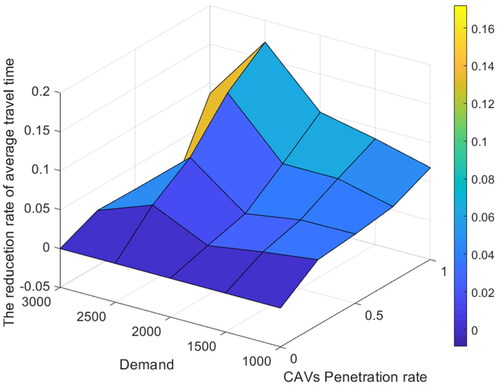
In summary, the results of the sensitivity analysis have demonstrated that system efficiency can still be improved by the ORST control strategy in mixed traffic conditions. The improvement is more significant at a high penetration rate of CAVs and a mild congestion level. This phenomenon is mainly caused by three factors. Firstly, when more CAVs are able to cooperate with other vehicles and signal controllers, the benefits of ORST control strategies are more significant. Secondly, when the road traffic system is highly congested, the improvement of optimization is limited by road capacity. Thirdly, when both CAVs and HDVs can travel in a free-flow condition, the improvement of ORST control strategies is not significant and is limited by the macroscopic fundamental diagram (MFD).

6. Conclusions

In this paper, the impacts of different driver information levels on routing and signal timing efficiency have been investigated, and the question of whether travel efficiency can be improved with information from CAVs has been answered.

As link travel cost $C_a(\mathit{v},\mathit{\psi })$ is influenced by link $a,$ link flow $\mathit{v}$ and signal setting $\mathit{\psi },$ the information about traffic conditions has been divided into three categories, including information about the network, traffic flow and signal setting. Four existing routing and signal timing strategies under different levels of information and a proposed ORST control strategy for CAVs have been compared on the same simple road network. The results of the simulation and sensitivity analysis demonstrated that with the increase of information levels, total travel time can be reduced with proper routing and signal timing strategies.

The primary contributions of this research can be summarized as follows. Firstly, the impacts of information levels on routing and signal timing efficiency have been investigated quantitatively. The results demonstrate that different levels of information will lead the road traffic system to different equilibrium points. With more accurate information about the traffic conditions, total travel time can be reduced, which is also the reason why traffic guidance systems have been developed to reduce congestion.

Secondly, to reduce total travel time with information from CAVs, an ORST control strategy for CAVs has been proposed. Compared with existing routing and signal timing strategies, the ORST can further reduce the total time to achieve Wardrop’s second equilibrium with additional information from CAVs.

Thirdly, the sensitivity analysis of ORST under different demands and CAVs penetration rates demonstrates that when only part of vehicles in the system can behave cooperatively, system efficiency can still be improved with ORST and the improvement is more significant at a high penetration rate and a mild congestion level.

Disclosure statement

No potential conflict of interest was reported by the authors.

Additional information

Funding

This work was funded by China Scholarship Council, 201708060287.

References

- Allsop, R., & Charlesworth, J. (1977). Traffic in a signal-controlled road network: An example of different signal timings including different routeing. Traffic Engineering & Control, 18, 262–264.
- Allsop, R. E. (1974). Some possibilities for using traffic control to influence trip distribution and route choice. 6th International Symposium on Transportation and Traffic Theory, New South Wales.
- Beckmann, M., McGuire, C. B., & Winsten, C. B. (1956). Studies in the economics of transportation. Yale University Press. http://cowles.yale.edu/sites/default/files/files/pub/misc/specpub-beckmann-mcguire-winsten.pdf
- Bifulco, G. N., Cantarella, G. E., Simonelli, F., & Velonà, P. (2016). Advanced traveller information systems under recurrent traffic conditions: Network equilibrium and stability. Transportation Research Part B: Methodological, 92, 73–87. https://doi.org/10.1016/j.trb.2015.12.008
- Cantarella, G. E., Improta, G., & Sforza, A. (1991). Iterative procedure for equilibrium network traffic signal setting. Transportation Research Part A: General, 25(5), 241–249. https://doi.org/10.1016/0191-2607(91)90141-C
- Chai, H., Zhang, H. M., Ghosal, D., & Chuah, C.-N. (2017). Dynamic traffic routing in a network with adaptive signal control. Transportation Research Part C: Emerging Technologies, 85, 64–85. https://doi.org/10.1016/j.trc.2017.08.017
- Chen, O. J. (1998). Integration of dynamic traffic control and assignment. Massachusetts Institute of Technology.
- Cheng, Y., Hu, X., Chen, K., Yu, X., & Luo, Y. (2022). Online longitudinal trajectory planning for connected and autonomous vehicles in mixed traffic flow with deep reinforcement learning approach. Journal of Intelligent Transportation Systems, 1–15. https://doi.org/10.1080/15472450.2022.2046472
- Chiou, S. W. (1999). Optimization of area traffic control for equilibrium network flows. Transportation Science, 33(3), 279–289. https://doi.org/10.1287/trsc.33.3.279
- Chiou, S. W. (2003). TRANSYT derivatives for area traffic control optimisation with network equilibrium flows. Transportation Research Part B: Methodological, 37(3), 263–290. https://doi.org/10.1016/S0191-2615(02)00013-9
- Daganzo, C. F., & Sheffi, Y. (1977). On stochastic models of traffic assignment. Transportation Science, 11(3), 253–274. https://doi.org/10.1287/trsc.11.3.253
- Dial, R. B. (1971). A probabilistic multipath traffic assignment model which obviates path enumeration. Transportation Research, 5(2), 83–111. https://doi.org/10.1016/0041-1647(71)90012-8
- Dijkstra, E. W. (1959). A note on two problems in connexion with graphs. Numerische Mathematik, 1(1), 269–271. https://doi.org/10.1007/BF01386390
- Fisk, C. (1980). Some developments in equilibrium traffic assignment. Transportation Research Part B: Methodological, 14(3), 243–255. https://doi.org/10.1016/0191-2615(80)90004-1
- Guo, Q., Li, L., & Ban, X. (2019). Urban traffic signal control with connected and automated vehicles: A survey. Transportation Research Part C: Emerging Technologies, 101, 313–334. https://doi.org/10.1016/j.trc.2019.01.026
- He, X., Guo, X., & Liu, H. X. (2010). A link-based day-to-day traffic assignment model. Transportation Research Part B: Methodological, 44(4), 597–608. https://doi.org/10.1016/j.trb.2009.10.001
- Heydecker, B. G. (1983). Some consequences of detailed junction modeling in road traffic assignment. Transportation Science, 17(3), 263–281. https://doi.org/10.1287/trsc.17.3.263
- Hu, X., & Sun, J. (2019). Trajectory optimization of connected and autonomous vehicles at a multilane freeway merging area. Transportation Research Part C: Emerging Technologies, 101, 111–125. https://doi.org/10.1016/j.trc.2019.02.016
- Kennedy, J., & Eberhart, R. (1995). Particle swarm optimization. Proceedings of ICNN'95-International Conference on Neural Networks.
- Li, T., Guo, F., Krishnan, R., Sivakumar, A., & Polak, J. (2020). Right-of-way reallocation for mixed flow of autonomous vehicles and human driven vehicles. Transportation Research Part C: Emerging Technologies, 115, 102630. https://doi.org/10.1016/j.trc.2020.102630
- Lopez, P. A., Behrisch, M., Bieker-Walz, L., Erdmann, J., Flötteröd, Y., Hilbrich, R., Lücken, L., Rummel, J., Wagner, P., & WieBner, E. (2018, Nov 4–7). Microscopic traffic simulation using SUMO. 2018 21st International Conference on Intelligent Transportation Systems (ITSC). https://doi.org/10.1109/ITSC.2018.8569938
- Maher, M. J., Zhang, X., & Vliet, D. V. (2001). A bi-level programming approach for trip matrix estimation and traffic control problems with stochastic user equilibrium link flows. Transportation Research Part B: Methodological, 35(1), 23–40. https://doi.org/10.1016/S0191-2615(00)00017-5
- Meneguzzer, C. (1995). An equilibrium route choice model with explicit treatment of the effect of intersections. Transportation Research Part B: Methodological, 29(5), 329–356. https://doi.org/10.1016/0191-2615(95)00011-2
- Milanés, V., & Shladover, S. E. (2014). Modeling cooperative and autonomous adaptive cruise control dynamic responses using experimental data. Transportation Research Part C: Emerging Technologies, 48, 285–300. https://doi.org/10.1016/j.trc.2014.09.001
- Mirheli, A., Hajibabai, L., & Hajbabaie, A. (2018). Development of a signal-head-free intersection control logic in a fully connected and autonomous vehicle environment. Transportation Research Part C: Emerging Technologies, 92, 412–425. https://doi.org/10.1016/j.trc.2018.04.026
- Olia, A., Razavi, S., Abdulhai, B., & Abdelgawad, H. (2018). Traffic capacity implications of automated vehicles mixed with regular vehicles. Journal of Intelligent Transportation Systems, 22(3), 244–262. https://doi.org/10.1080/15472450.2017.1404680
- Robertson, D. I. (1969). TRANSYT method for area traffic control. Traffic Engineering and Control, 11, 276–281.
- Smith, M. (2015). Traffic signal control and route choice: A new assignment and control model which designs signal timings. Transportation Research Part C: Emerging Technologies, 58, 451–473. https://doi.org/10.1016/j.trc.2015.02.002
- Smith, M. J. (1979a). The existence, uniqueness and stability of traffic equilibria. Transportation Research Part B: Methodological, 13(4), 295–304. https://doi.org/10.1016/0191-2615(79)90022-5
- Smith, M. J. (1979b). Traffic control and route-choice; a simple example. Transportation Research Part B: Methodological, 13(4), 289–294. https://doi.org/10.1016/0191-2615(79)90021-3
- Smith, M. J. (1981). The existence of an equilibrium solution to the traffic assignment problem when there are junction interactions. Transportation Research Part B: Methodological, 15(6), 443–451. https://doi.org/10.1016/0191-2615(81)90029-1
- Smith, M. J. (1984). The stability of a dynamic model of traffic assignment—An application of a method of Lyapunov. Transportation Science, 18(3), 245–252. https://doi.org/10.1287/trsc.18.3.245
- Smith, M. J., & Ghali, M. (1990). The dynamics of traffic assignment and traffic control: A theoretical study. Transportation Research Part B: Methodological, 24(6), 409–422. https://doi.org/10.1016/0191-2615(90)90036-X
- So, J., Hwangbo, J., Kim, S. H., & Yun, I. (2022). Analysis on autonomous vehicle detection performance according to various road geometry settings. Journal of Intelligent Transportation Systems, 1–12. https://doi.org/10.1080/15472450.2022.2042280
- Taale, H., & van Zuylen, H. J. (2001, July 22). The combined traffic assignment and control problem–an overview of 25 years of research 9th World Conference on Transport Research, Korea.
- Tajalli, M., & Hajbabaie, A. (2022). Traffic signal timing and trajectory optimization in a mixed autonomy traffic stream. IEEE Transactions on Intelligent Transportation Systems, 23(7), 6525–6538. https://doi.org/10.1109/TITS.2021.3058193
- Wang, Y., Wei, L., & Chen, P. (2020). Trajectory reconstruction for freeway traffic mixed with human-driven vehicles and connected and automated vehicles. Transportation Research Part C: Emerging Technologies, 111, 135–155. https://doi.org/10.1016/j.trc.2019.12.002
- Wardrop, J. G. (1952). Some theoretical aspects of road traffic research. Proceedings of the institution of civil engineers. https://doi.org/10.1680/ipeds.1952.11259
- Webster, F. V. (1958). Traffic signal setting. H.M.S.O.
- Xu, B., Ban, X. J., Bian, Y., Li, W., Wang, J., Li, S. E., & Li, K. (2019). Cooperative method of traffic signal optimization and speed control of connected vehicles at isolated intersections. IEEE Transactions on Intelligent Transportation Systems, 20(4), 1390–1403. https://doi.org/10.1109/TITS.2018.2849029
- Yang, H., & Yagar, S. (1994). Traffic assignment and traffic control in general freeway-arterial corridor systems. Transportation Research Part B: Methodological, 28(6), 463–486. https://doi.org/10.1016/0191-2615(94)90015-9
- Yang, H., & Yagar, S. (1995). Traffic assignment and signal control in saturated road networks. Transportation Research Part A: Policy and Practice, 29(2), 125–139. https://doi.org/10.1016/0965-8564(94)E0007-V
- Yu, C., Feng, Y., Liu, H. X., Ma, W., & Yang, X. (2018). Integrated optimization of traffic signals and vehicle trajectories at isolated urban intersections. Transportation Research Part B: Methodological, 112, 89–112. https://doi.org/10.1016/j.trb.2018.04.007