Revealing representative day-types in transport networks using traffic data clustering

Abstract

Recognition of spatio-temporal traffic patterns at the network-wide level plays an important role in data-driven intelligent transport systems (ITS) and is a basis for applications such as short-term prediction and scenario-based traffic management. Common practice in the transport literature is to rely on well-known general unsupervised machine-learning methods (e.g., k-means, hierarchical, spectral, DBSCAN) to select the most representative structure and number of day-types based solely on internal evaluation indices. These are easy to calculate but are limited since they only use information in the clustered dataset itself. In addition, the quality of clustering should ideally be demonstrated by external validation criteria, by expert assessment or the performance in its intended application. The main contribution of this paper is to test and compare the common practice of internal validation with external validation criteria represented by the application to short-term prediction, which also serves as a proxy for more general traffic management applications. When compared to external evaluation using short-term prediction, internal evaluation methods have a tendency to underestimate the number of representative day-types needed for the application. Additionally, the paper investigates the impact of using dimensionality reduction. By using just 0.1% of the original dataset dimensions, very similar clustering and prediction performance can be achieved, with up to 20 times lower computational costs, depending on the clustering method. K-means and agglomerative clustering may be the most scalable methods, using up to 60 times fewer computational resources for very similar prediction performance to the p-median clustering.

Keywords:

• Cluster validity
• clustering
• day clustering
• dimensionality reduction
• external indices
• internal indices
• network-wide
• prediction

1. Introduction

1.1. Background

Data-driven methods for Intelligent Transport Systems (ITS) are experiencing a significant boom in research and practice (Laña et al., 2021). Thanks to the expansion of cost-effective sensor networks on highways, public transport, urban streets, etc. as well as open-data initiatives that make traffic data sources widely accessible, huge flows of information and data are becoming the norm (Laña et al., 2021; Zhang et al., 2011). As ITS produce and require large amounts data, the field is becoming increasingly interdisciplinary, combining traffic engineering with machine learning, artificial intelligence, and data science (Zhu et al., 2018). Recently, data-driven ITS have been defined by Zhang et al. (2011) as ITS where data-driven methods and learning algorithms play a key role in optimizing the system performance. There remain many challenges as well as opportunities in data-driven ITS (Zhu et al., 2018) concerning big data and their utilization in strategic, tactical, and operational real-time management planning.

Historical traffic or travel patterns are key ingredients in ITS for the estimation and prediction of demand and traffic states. According to Laña et al. (2021) it is beneficial to reveal regularities in historical traffic profiles and use them as the basis before applying regression or other prediction models. This paper focuses on revealing sets of representative day-types with data-driven clustering methods, for the purpose of ITS applications. Days represent an appropriate time unit in transport networks as traffic conditions, such as congestion, from one day to the next are relatively independent, which is not the case for shorter within-day periods (hours or minutes). We refer to traffic pattern clustering at the day level as day clustering. Ideally, these day-types capture regularities or typicalities in the form of representative network-wide historical patterns. Furthermore, they may serve as a basis for predicting the future states of the network on a given day. The application of the set of day-types can vary from strategic transport and urban planning, to real-time and scenario-based traffic management.

The set of representative day-types can be determined using varying clustering methods, similarity or distance measures among days, and with a varying number of clusters (Estivill-Castro, 2002). Each cluster would then represent one representative network-wide day-type. Many different cluster validity indices or evaluation metrics could be used for selecting the clustering which best matches the criteria. Common practice is to use one of the well-known and widely accepted clustering methods such as k-means, hierarchical, affinity propagation, or spectral clustering (Lopez et al., 2017; Yang et al., 2017; Krishnakumari et al., 2020; Ferranti, 2020; Cebecauer et al., 2019; Chiabaut & Faitout, 2021).

The number of clusters is generally decided by using internal evaluation indices, which evaluate the clustering structure using only information in the clustered dataset itself. This enables the discovery of natural structures in the dataset, but the performance in their intended application is not considered. In this paper we extend this by proposing an external evaluation method using short-term prediction performance as criterion of validity. Prediction is used as the application of the day-types, but also as a proxy for the performance of the day-types in data-driven ITS applications more generally. The external and internal validation results are then compared, and we investigate to what degree internal evaluation criteria provide sufficient information to provide day-type clusterings that are useful in prediction applications, and where external validation produces different results.

The main focus of the paper is to determine the most representative day-types in the network, as well as to propose a data-driven clustering-based prediction model that enhances the performance of both simple and more complex prediction models. The paper highlights the importance of not relying only on internal evaluation indices when determining the most appropriate clustering but also the application’s performance. Considering only application performance can result in a very high number of clusters, while internal evaluation indices usually point to low numbers of clusters. Moreover, various internal indices may indicate different numbers of clusters, making it difficult to determine a clear selection. We show the importance of combining both internal indices to reveal natural clusters and their performance in the short-term prediction application when determining the most representative set of day-types in the network.

1.2. Literature review and state-of-the art

Clustering is a classic research problem with applications in many fields, in particular where huge amounts of data are available. In general, clustering aims to group data or entities considering their attributes, in a way that the difference or variance within each cluster is minimized and the dissimilarity or distance between distinct clusters is maximized. Since the notion of what a cluster is varies depending on data and applications, there are many different clustering algorithms used in data science and machine learning (Estivill-Castro, 2002). Further, principles and models can often be solved only approximately with heuristics, and thus there is an even larger number of algorithms (Estivill-Castro, 2002). However, some clustering methods and algorithms are more popular for handling large amounts of data in multidimensional spaces, including k-means (MacQueen et al., 1967), hierarchical (Murtagh, 1983), affinity propagation (Frey & Dueck, 2007), DBSCAN (Ester et al., 1996), and spectral clustering (Shi & Malik, 2000). Despite their widespread use, according to Adolfsson et al. (2019) there is still debate about which algorithm should be used in which circumstances. The problem is even more complex as clustering methods usually rely on a similarity or distance metric. Among the many metrics that could be used, the most prevalent for day clustering in transport networks are the Euclidean distance (Cebecauer et al., 2019; Lopez et al., 2017; Yang et al., 2017), cosine similarity (Cebecauer et al., 2019; Toqué et al., 2017), and normalized mutual information (Chiabaut & Faitout, 2021; Krishnakumari et al., 2020; Lopez et al., 2017).

Evaluating and selecting the most appropriate clustering for a dataset can be at least as challenging as the clustering itself (Pfitzner et al., 2009). To choose among the clustering methods and number of clusters there are many evaluation methods available (Adolfsson et al., 2019). While the choice should reflect the purpose and application of the clustering, popular methods tend to be similar in their objective to commonly used clustering methods like k-means and DBSCAN, and use distances, variances and densities for evaluating the suitability of the clustering. Estivill-Castro (2002) shows that clustering methods that have the same or similar criteria as the validation index will perform very well compared to those that do not. According to Rendón et al. (2011) these evaluation indices can be categorized into two main groups, internal and external evaluation. Internal evaluation indices, such as Silhouette index, Dunn index, within-cluster variance, cluster dissimilarity, and Composing Density between and Within cluster (CDbW), use only information in the dataset that is clustered. External evaluation indices, such as F-measure, Purity, Entropy, Rand index, Jaccard index, Dice index, and normalized mutual information, may use additional information.

A different approach for clustering is to define the objective function that best matches the application purpose and propose a heuristic or exact solution algorithm (Estivill-Castro, 2002). This approach is common in fields such as operations research, for example in location-allocation analysis. Methods with different objectives and available exact methods are good candidates to consider in network-wide day clustering along with the commonly used general clustering methods. Challenges come from the complexity of translating the application into a mathematical model, which is likely to fall into the class of NP-hard problems.

According to (Estivill-Castro, 2002; Feldman et al., 2007) the quality of clustering should ideally be demonstrated by external validation criteria, by expert assessment or the utility in its intended application. Furthermore, best practice would be to formulate mathematically explicit models and propose a clustering algorithm to match this criterion. Considering the complexity of transport networks and traffic (Laña et al., 2021), it is not surprising that the choice in many cases relies on selecting one or a few of the commonly used clustering methods and internal evaluation metrics (Chiabaut & Faitout, 2021; Krishnakumari et al., 2020; Lopez et al., 2017; Toqúe et al., 2017; Yang et al., 2017). Usually, the purpose or the application of the clustering is not considered. Evaluation toward application is usually limited to performance demonstration of the selected clustering (method and number of clusters, selected by internal evaluation only) in for example short-term prediction (Chiabaut & Faitout, 2021; Krishnakumari et al., 2020; Lopez et al., 2017; Toqúe et al., 2017).

With increasing data availability and advances in machine learning, artificial neural networks and deep learning methods are becoming popular (van Lint & van Hinsbergen, 2012; Van Hinsbergen et al., 2007; Vlahogianni et al., 2014; Zhang et al., 2021). Long-Short Term Memory (LSTM) recurrent neural networks are used for OD flow matrices in Ferranti (2020); Toqué et al. (2017)). Patel et al. (2022) proposed metaheuristic enabled deep convolution neural network for traffic flow prediction and compared several different machine learning and artificial intelligence prediction models (based on: Support Vector Machine, Back Propagation Neural Networks, Convolutional Neural Networks, Deep Belief Networks, Recurrent Neural Networks, Gradient Descent, Particle Swarm Optimization, and Lion Algorithm) across 33 datasets. Ferranti (2020) uses AutoRegressive Integrated Moving Average (ARIMA) for short-term prediction of OD flows. Zhang et al. (2021) uses deep learning methods for short-term OD flow prediction and gives an extensive literature review of recent methodological developments. Random forests are used in Toqué et al. (2017), ARIMA models are used in Ferranti (2020); Kumar and Vanajakshi (2015), and vector autoregression (VAR) is used in Ferranti (2020). A hybrid method of exponential smoothing and probabilistic principal component analysis (PPCA) is introduced in Jenelius and Koutsopoulos (2018) for short-term speed and travel-time prediction. This hybrid PPCA model is extended to exponential smoothing for connected neighborhoods in Cebecauer et al. (2019). The benefits of spatial clustering for short-term travel-time prediction with PPCA are demonstrated in Cebecauer et al. (2018). Exponential smoothing in combination with day clustering is also used in Chrobok et al. (2004).

It is essential to highlight that clustering large datasets to smaller, more homogeneous spatial neighborhoods, day-type, and spatio-temporal clusters may be useful as a general methodology for improving both computational and prediction performance of already existing prediction models and thus has considerable potential Laña et al. (2021). Hence, it is not surprising that it is common in the research literature concerning prediction in transportation networks to limit case studies to weekdays that are not school or public holidays. There are two main motivations behind this: most prediction models benefit from a more homogeneous subset of data, and it represents relevant days when prediction could be most needed. This subset of days with expected similarity combines calendar knowledge with some expertise in traffic and case study areas. In this paper, we refer to this day selection as calendar-based day clustering.

To this date only a few studies use network-wide day clustering as the basis for further prediction (Cebecauer et al., 2019; Chiabaut & Faitout, 2021; Krishnakumari et al., 2020; Lopez et al., 2017; Toqúe et al., 2017). According to Van Hinsbergen et al. (2007) this is usually limited to naïve prediction models such as historical mean used also in the most of the current day clustering literature. The early cluster-based prediction models, such as Wild (1997) and Chrobok et al. (2004), have focused on optimizing short-term prediction performance and resulted in 60 - 200 daily patterns for one calendar year. However, with this paper we aim to reveal the representative ”natural” day-types in the transportation network, which is in line with current day-clustering literature, while also taking into consideration the prediction performance in the application. Current literature uses the short-term prediction performance to demonstrate performance in the application, considering only number of representative day-types determined by internal indices (Chiabaut & Faitout, 2021; Krishnakumari et al., 2020; Lopez et al., 2017). Lopez et al. (2017) introduced congestion maps and consensual days for capturing similarities in traffic condition and dynamics and demonstrated in a short-term prediction application. Meanwhile, Cebecauer et al. (2019) shows that congestion maps and consensual days can be outperformed by mean day-type vectors if extensive external evaluation for short-term prediction is not considered. Furthermore, both consensual days and mean day-types can outperform PPCA used on day non-clustered datasets. The methodology of Lopez et al. (2017) has been adopted and improved for short-term prediction in Krishnakumari et al. (2020) by introducing shapes for representing network traffic dynamics. Chiabaut and Faitout (2021) noted that different internal indices criteria are not consistent among them and have different objectives, which leads them to tailor new metrics to determine the appropriate number of day clusters. Table 1 summarizes the above literature concerning day-type clustering and using day-types as basis for training prediction models.

Table 1. Summary table of network-wide day clustering.

Data Type	Internal	Clustering	Classification	Similarity	Centroid	Dimensionality reduction	Train set [days]	Test set [days]	Prediction model	Paper
speed	TWCV, TCD	k-means, spectral, DBSCAN	ED	MI	Consensus	–	35	1	centroid-based	Lopez et al. (2017)
speed, flow	TWCV, TCD	k-means, spectral	ED	MI, AMI,CS	Consensus, historical-mean	–	127	30	centroid-based	Cebecauer et al. (2019)
speed	TWCV, TCD	k-means	ED	MI	Consensus, shape-based, historical-mean	PCA	34	35 × 1	centroid-based	Krishnakumari et al. (2020)
speed	TWCV, TCD, SC	k-means, GMM	ED	MI	Consensus	PCA	167	56	centroid-based	Chiabaut and Faitout (2021)
speed, flow	TWCV	Two-step(calendar, agglomerative)	–	Ward	–	–	118	–	–	W. Weijermars and Van Berkum (2005)
flow	–	Two-step (calendar, gravitational)	calendar & maximal vertical difference	=classi.	Historical-mean	–	42	10	trivial, moving average, exponential smoothing	Wild (1997)
flow	SC, DB, CH	spectral, affinity propagation	–	ED	–	PCA, SVD	290	–	–	Yang et al. (2017)
flow	–	calendar	mean ED	=classi.	–	–	730	52	exponential smoothing, linear curve fitting	Chrobok et al. (2004)
flow	–	calendar	calendar, RF	–	–	–	361	359	LSTM, RF	Toqué et al.,(2017)
flow	TWCV	calendar, k-mean	calendar, ED	ED	Historical-mean	PCA, SVD	212	54	centroid-based, Persistence method, ARIMA, VAR	Ferranti (2020)
speed, flow	calendar	calendar	calendar	–	–	–	21	7	Multivariete nonparametric regression	Clark (2003)

Table uses followint abbrevations: Silhouette Score (SC), Davies-Bouldin index (DB), Euclidean Distance (ED), Gaussian Mixture Model (GMM), Mutual Information (MI), Adjusted Mutual Information (AMI), Cosine Similarity (CS), Calinski-Harabasz(CH), Random forest (RF) Long-Short Term Memory (LSTM), Autoregressive Integrated Moving Average method (ARIMA), Vector Autoregression method (VAR).35x1 for Test dataset in Krishnakumari et al. (2020) refers to leave-one-out strategy for all 35 days.

When dealing with large networks or large OD matrices, the measurement vector representing one day can easily exceed a hundred thousand dimensions. Dimensionality reduction is a proven technique in the transport literature (Djukic et al., 2012; Krishnakumari et al., 2020; Yang et al., 2017) and reduces the problem size while preserving most of the information. The most widely used dimensionality reduction method is Principal Component Analysis (PCA), which has already been used in day clustering (Djukic et al., 2012; Ferranti, 2020; Krishnakumari et al., 2020; Luo et al., 2017; Yang et al., 2017). It has been shown that dimensionally reduced datasets with only few principal components can effectively contain a great amount of variance (information) (Djukic et al., 2012; Luo et al., 2017).

To the best of our knowledge, the existing transport related literature usually evaluates day-type clustering by internal evaluation methods only. While internal evaluation is important, it is often isolated from the application and can only provide limited insight into whether some algorithm or number of clusters performs better than another. Thus, internal evaluation does not necessarily imply that one clustering is more valid than another (Estivill-Castro, 2002). However, the approach is becoming general practice for travel pattern clustering, even if the application or its proxy in the form of external evaluation can be used. Therefore, it is important to consider external evaluation, which reflects its utility in its intended application (Estivill-Castro, 2002; Feldman et al., 2007).

1.3. Contribution of the paper

The main contribution of the paper is to put the practice of internal clustering evaluation methods and general clustering algorithms to the test with external evaluation. Many applications in ITS and traffic management on a network-wide level, including short-term prediction, may require some level of clustering of data by day-types in order to provide satisfactory performance. In this work we use two relatively simple prediction schemes as proxy for a larger range of ITS applications, including more sophisticated prediction schemes and real-time and predictive traffic signal control, as well as scenario-based traffic management. We evaluate how the recognized representative patterns selected by clustering and internal evaluation indices perform in such forecasting applications.

The determination of the day-type clustering should consider three aspects: identify natural clusters recognized by internal evaluation indices; evaluate the performance in the short-term prediction performance; and ideally at the end it should be evaluated by expert(s) with knowledge of the traffic in the concerned transport network. This is also generally suggested in the clustering literature (Estivill-Castro, 2002; Feldman et al., 2007).

We propose to use short-term prediction as a general proxy for external evaluation of clusters for other ITS applications. The case study in this paper considers flow data collected during the years 2017 and 2018 by microwave detectors on motorways in Stockholm, Sweden. In literature (Manibardo et al., 2021), at least two years of data, when the first is used for training and second for evaluation, is considered sufficient.

There are three additional contributions of this paper. First, the paper also investigates the impacts of the determined day-types and their numbers on the short-term prediction application.

Second, we explore the benefits of data-driven day clustering compared to calendar-based clustering. Clusterings that separate working days from weekends and holidays are very common practice in short and long-term prediction, and examples of finer granularity also exist (Toqué et al., 2016; Toqué et al., 2017). It is expected that data-driven day clustering achieves better performance than calendar-based clustering across all internal and external evaluation methods.

Third, the paper investigates the benefits for internal and external evaluation of performing dimensionality reduction on the original dataset. To the best of our knowledge, this has not been adequately analyzed in the context of day clustering in transport networks. We expect two possible outcomes. On the one hand, because of the curse of dimensionality, the dimensionality reduction can improve the external evaluation metric. On the other hand, some of the important information may be lost and result in worse external evaluation performance.

Considering the general contributions of the paper, we formulate the following research questions:

• Do internal and external evaluation result in the same selection of clusters?

• What is the impact of day-type clusters and their number on short-term prediction performance?

• What is the performance and computational cost of commonly used clustering algorithms considering internal and external evaluation?

• Does data-driven day clustering outperform basic calendar-based clustering?

• What is the impact of dimensionality reduction on the internal and external evaluation methods?

The remainder of the paper is organized as follows. Section 2 describes the overall methodology framework with clustering, internal evaluation, and short-term prediction as external evaluation. The case study and computational experiments designed to answer the research questions are introduced in Section 3. The results are presented in Section 4. Section 6 summarizes our conclusions and future research directions.

2. Methodology

2.1. Framework

This section introduces the methodological framework for unveiling a representative set of day-types for a transport network, i.e., the most frequently occurring day patterns. We assume that at least a year’s worth of data is available. Across a whole year, there are many levels of traffic profiles and patterns in complex transport networks (W. A. M. Weijermars, 2007), ranging from seasonal cycles, school and public holidays, variations across working days and weekends, to intra-day variations between early morning, morning peak, between peaks, afternoon peak, night, etc. The framework is summarized in Figure 1. The notation used in the paper is summarized in Table 2.

Figure 1. Overview of the methodological framework for revealing the representative set of day-types Y with internal and external evaluation, including dimensionality reduction, day clustering. External evaluation process is highlighted.

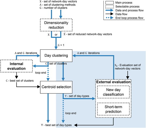
Table 2. Notation

Notation	Description
d	Index of day
N	Number of days or network-day vectors
$N_T$	Set of training days
$N_C$	Set of calibration days
$N_E$	Set of evaluation days
j	Index of time interval
J	Number of time intervals
i	Index of observation entity
I	Number of observation entities in the network
X	matrix with network-day vectors
$X_T$	matrix of network-day vectors in set $N_T$
$X_C$	matrix of network-day vectors in set $N_C$
$X_E$	matrix of network-day vectors in set $N_E$
$x_d$	Network-day vector of day d
$v_{ij}^{x_d}$	Observation on network-day vector $x_d$ of day d at time interval j and observation entity i.
$v_m^{x_d}$	Observation at the m dimension of the network-day vector $x_d$ of day d.
M	Number of dimensions, $M=I\times J$
G	Number of day clusters
C	Set of G clusters $C=\{C_1,C_2,\dots ,C_G\}$
$y_g$	Centroid of the cluster g (day-type)
$y_{(}g,i,j)$	Value of centroid g for observation entity i and interval j
Y	Set of clusters’ centroids (day-types)
R	Maximal number of past intervals to be consider in classification and local smoothing
f	Index of future time interval
F	Set of future time intervals to be considered in prediction and calibration

We formalize a network-day as a space-time ordered vector. With “space” we refer to observation entities that have a geographical placement in the network and can represent a point (sensor), link or route (pair of sensors), or origin-destination pair. These entities are sources of traffic state observations and can be used to measure flows, speeds, travel times, or densities. Let the network be represented by I observation entities. For each observation entity $i\in I,$ measurements are collected and aggregated for J time intervals. The time interval can be any period, e.g., 5 min, 15 min, 1 h, or 24 h depending on the application. If a fine granularity is used, e.g. 15 min or less, travel patterns within the day can be captured in the clustering.

Let network-day d be represented by the ordered space-time series vector $x_d,$ consisting of all observations $v_{ij}^{x_d}$ during time intervals $j=1,\dots ,J$ observed in the transport network represented by observation entities $i=1,\dots ,I$. Let $M=I\times J$ denote the number of features of the vector $x_d,$ which can be written as: (1) $$x_d=(v_{1,1}^{x_d},\dots ,v_{I,1}^{x_d},v_{1,2}^{x_d},\dots ,v_{I,2}^{x_d},\dots ,v_{1,J}^{x_d},\dots ,v_{I,J}^{x_d})=(v_1^{x_d},\dots ,v_M^{x_d}).$$(1)

Now, we define the dataset X of all historical N network-day vectors as a matrix with N rows and M columns (dimensions): (2) $$X=\left(\begin{array}{c}{x}_1\\ x_2\\ \dots \\ x_N\end{array}\right)=\left(\begin{array}{c}{v}_1^{x_1},\dots ,v_M^{x_1}\\ v_1^{x_2},\dots ,v_M^{x_2}\\ ⋮ , \dots , ⋮\\ v_1^{x_N},\dots ,v_M^{x_N}\end{array}\right)$$(2)

To reveal day-types we group network-days that have a similar pattern across their M dimensions. Although similarity can be expressed in various ways, this paper adopts the commonly used Euclidean distance.

Especially for large networks, the number of dimensions can greatly exceed the number of observed days. Furthermore, some intervals exhibit low variance, in particular during night or mid-day and for observations entities that do not experience congestion. The idea behind dimensionality reduction is that the variance in the spatio-temporal data may be sufficiently explained by a lower number of dimensions. Thus, we investigate the impact of dimensionality reduction prior to the clustering. All experiments are presented in parallel with the original dataset X on the one hand and a dimensionally reduced dataset $\overline{X}$ on the other hand.

For dimensionality reduction we use principal component analysis (PCA). PCA generates linearly uncorrelated orthogonal axes, also known as principal components in the M-dimensional space. Any network-day vector $x_d$ in the original space can be projected to the new natural coordinate system. The principal components are ordered based on the explained variance of the training data set X. It is common practice to select principal components that explain 90% of the variance (Djukic et al.,2012).

Clustering groups the N days of dataset X into G clusters $C=\{C_1,C_2,\dots ,C_G\},$ where $X=C_1\cup C_2\cup \dots \cup C_G$ and $C_1\cap C_2\cap \dots \cap C_G=.$ Thus, each cluster $C_g\in C$ is a subset of $\left|C_g\right|$ network-day vectors. We introduce several candidate clustering algorithms in Subsection 2.2.

For each cluster, the representative day-type is selected, referred to as the centroid of the cluster. To allow comparison across different clustering methods, we define the day-type of the cluster $C_g\in C$ as the mean network-day vector $y_g.$ Thus, the set $Y=\{y_1,y_2,\dots ,y_G\}$ is the set of the representative day-types for clustering $C=\{C_1,C_2,\dots ,C_G\}$ of the dataset X. The observation values in centroid vector $y_g$ are calculated for all the dimensions $i=1,\dots ,I$ and $j=1,\dots ,J$ as the mean values across days in cluster $C_g:$ (3) $$v_{ij}^{y_g}=\frac{\sum _{d\in C_g}{v}_{ij}^{x_d}}{\left|C_g\right|}$$(3)

This simple approach is robust in terms of both performance and computation (Cebecauer et al., 2019).

To evaluate clustering performance and select the best performing method and number of clusters, several commonly used internal validation indices are described in Section 2.3. In Section 2.4 we propose a novel approach to external evaluation of network-wide day clustering performance based on the application to short-term prediction.

2.2. Day clustering

2.2.1. Calendar-based clustering

As baseline in the evaluation of data-driven clustering methods we use calendar-based clustering. While data-driven clustering uses real-world observations, calendar-based clustering uses only knowledge about the days: day-of-week, weekend, school and public holidays, de-facto holidays, and their combinations. We define three main sets of calendar-based clustering categories in Table 3.

Table 3. Sets of calendar-based clustering categories.

Abbreviation	Full name	Cluster’s categories description
dow	day-of-week	Monday, Tuesday, Wednesday, Thursday, Friday, Saturday, Sunday
wkd	weekend/weekday	Monday – Friday, Saturday – Sunday
hol	holiday	No holiday, Public holiday, School holiday, De-facto holiday

The calendar-based clustering methods considered are denoted ${\text{cal}}_{\text{dow}},$ ${\text{cal}}_{\text{wkd}\times \text{hol}},$ and ${\text{cal}}_{\text{dow}\times \text{hol}}$ , where $\times$ indicates the cartesian product off the sets of calendar categories. The clustering ${\text{cal}}_{\text{dow}}$ does not recognize any holidays or special days. The clustering ${\text{cal}}_{\text{wkd}\times \text{hol}}$ does not distinguish day-of-week but separates weekends from weekdays, as well as if they are during school or public holidays. The most disaggregate calendar-based clustering ${\text{cal}}_{\text{dow}\times \text{hol}}$ distinguishes both individual weekdays and the type of holiday.

2.2.2. Data-driven clustering

We use two main groups of data-driven clustering methods. The first group consists of heuristic methods from machine learning, in particular k-means, hierarchical clustering, and spectral clustering. The objective of the clustering methods is usually to both minimize the variance within clusters and maximize the dissimilarity among the clusters. However, the heuristic algorithms cannot guarantee the optimality and quality of the resulting clusters, and some of the algorithms approximate the true clustering objective function for better computational performance. Below, we briefly introduce the clustering methods; for more detailed formulations of each method we refer to supplementary file S1.

K-means clustering is a well-known multidimensional clustering method (MacQueen et al., 1967) that attempts to create a set of clusters C that is efficient with respect to within-cluster variance. The formulation is NP-hard, but the very efficient approximative Lloyd’s algorithm (Lloyd, 1982) is widely used.

Agglomerative clustering with “ward” linkage (Ward, 1963) is a “bottom-up” hierarchical clustering approach where at the start each day in the dataset is represented by one cluster and then iteratively merges the pairs of clusters that minimally increase the total within-cluster variance. This approach is based on variance minimization and thus it is similar to the objective function in k-means clustering.

Spectral clustering is a graph partitioning algorithm designed for image segmentation (Shi & Malik, 2000), but also widely used in transport network partitioning (Ji & Geroliminis, 2012; Lopez et al., 2017; Saeedmanesh & Geroliminis, 2016). The approach proposed by Shi and Malik (2000) is based on concepts from spectral graph theory and uses eigenvalues and eigenvectors to bipartition the graph. Using the nearest neighborhood graph of dataset X, the problem is equivalent to the minimal cut in the graph. We refer to this variant of spectral clustering as ”${\text{spectral}}_{\text{NN}}$” (it can also use a precomputed affinity or similarity matrix). The second variant denoted as ”${\text{spectral}}_{\text{CS}}$”, used in Cebecauer et al. (2019), uses the similarity matrix calculated as cosine similarity between two network-day vectors $x_{d_1}$ and $x_{d_2}.$ The third variant ”${\text{spectral}}_{\text{AMI}}$”, introduced in Lopez et al. (2017), uses a similarity matrix calculated with adjusted mutual information (AMI). First, for each day vector $x_d\in X,$ the k-mean spatio-temporal clustering is performed. The AMI then calculates the mutual information between two days $d_1$ and $d_2$ using the spatio-temporal cluster label information instead of absolute values. Furthermore, the original methodology for ${\text{spectral}}_{\text{AMI}}$ has mostly been used for speeds and connected networks (Chiabaut & Faitout, 2021; Krishnakumari et al., 2020; Lopez et al., 2017).

As a second group of clustering methods, we consider exact and approximative methods from location-allocation analysis, which can guarantee optimal or high-quality solutions considering their objective function. The first approach is commonly referred to as p-median (also: minimum facility location, or Weber problem). The NP-hard problem aims to establish G centroids in such a way that the total multidimensional distance between the network-day vectors and the closest centroids is minimized. We use the exact algorithm ZEBRA (García et al., 2011) (Z-Enlarge-and-BRanch-Algorithm) for solving this optimal clustering problem.

In contrast, lexicographic minimax considers the utility of each network-day vector $x\in X$ in the form of its distance to the closest centroid and aims to establish a fair “pareto optimal” solution among these vectors. Lexicographic minimax does not intend to minimize the within-cluster variance as in many other machine-learning clustering algorithms. On the other hand, it is expected that the cluster dissimilarity will be larger compared to other methods and result in more robust day-type vectors that better distinguishes more distant or outlier days. For solving the lexicographic minimax problem, we use the very efficient approximative algorithm a-lex (Buzna et al., 2014).

2.3. Internal evaluation of day clustering

Validation indices are used to identify the best performing clustering methods and number of clusters. Two basic evaluation indices used also in Lopez et al. (2017) and Chiabaut and Faitout (2021) are Total Within Cluster Variance (TWCV), and Total Cluster Dissimilarity (TCD). In this paper we consider two that account for both cohesion (similarity within the cluster) and separation (dissimilarity with other clusters) such as: silhouette score (SC) (Rousseeuw, 1987), and Davies-Bouldin (DB) index (Davies & Bouldin, 1979). Silhouette score is also used in Chiabaut and Faitout (2021) when determining the number of day-type clusters. We refer readers to the supplementary information file S1 for exact definition and formulation of the indices used in this paper.

2.4. External evaluation based on short-term prediction

Short-term prediction as external evaluation aims to quantify the ability of the clustering C and its centroids Y to match the patterns of new days (future days or selected evaluation days, referred to as dataset $X_E$ in this work). This approach also evaluates the ability of the clustering C to be used for network-wide traffic prediction. The dataset X is split into a training dataset $X_T$ and an evaluation dataset $X_E.$ The best performing clustering on the evaluation set $X_E$ (algorithm in combination with number of clusters) is selected.

The process for this evaluation is divided into a number of subproblems: day classification, short-term prediction, and prediction performance evaluation. For a specific time interval j, each network-day vector in an evaluation dataset $x_d\in X_E$ is first classified to one of the G clusters. There are multiple ways of classifying a new day $d\in N_E$ into one of the G clusters. One commonly used approach in the transport field is to pick the closest cluster by considering one of many distance metrics (Cebecauer et al., 2019; Djukic et al., 2012; Lopez et al., 2017). We will use the Euclidean distance metric, which is commonly used in transport research and practice.

To formulate the classification model with Euclidean distance we first denote the classification model as a function $\Phi (Y,x_d,j,r_j)$ that returns the closest centroid vector $y_g$ to the new day vector $x_d.$ The inputs of function $\Phi$ are the set of the centroids Y of clustering C, the new network-day vector $x_d,$ the current time interval j, and the $r_j$ past intervals calibrated for time interval j. The classification model is formulated as follows: (4) $$\Phi (Y,x_d,j,r_j)=\arg \underset{y_g\in Y}{\min }\sqrt{\sum _{i=1}^I\sum _{l=1}^{\min \{r_j,j\}}{(v_{i,j+1-l}^{y_g}-v_{i,j+1-l}^{x_d})}^2}$$(4)

The centroid day-type vector $y_g$ serves the purpose of being the basis for the prediction of the future time intervals $f>j$ of day d. All predictions beyond time interval j for the whole network represented by I observation entities and F future time intervals are as follows: (5) $${\widehat{v}}_{if}^{x_d}:=v_{if}^{\overline{y}}, i=1,\dots ,I;f=j,\dots ,j+F$$(5)

While there are several prediction performance metrics, we propose to use the relative Mean Absolute Percentage Error (MAPE) metric for evaluation dataset $X_E$ across all day-time intervals J, observation entities I, and F future day-time intervals for evaluating clustering C. The MAPE is defined in our case as follows: (6) $$\text{MAPE}=\frac{1}{J}\sum _{j=1}^J\frac{1}{N_E}\sum _{d=1}^{N_E}\frac{1}{I}\sum _{i=1}^I\frac{1}{F}\sum _{f=1}^{\min \{F,J-j\}}\frac{|v_{i,j+f}^{x_d}-{\widehat{v}}_{i,j+f}^{x_d}|}{v_{i,j+f}^{x_d}}$$(6)

We also extend the short-term prediction that relies only on cluster centroids $y_g\in Y$ with an exponential smoothing stage. This approach has been used before in the transport literature to enhance the accuracy and robustness of predictions by smoothing across past time intervals (Jenelius & Koutsopoulos, 2018) or spatial neighborhoods (Cebecauer et al., 2017). The exponential smoothing considers the residuals between observed values in the R past time intervals of each day and the selected day-type vector $y_g,$ and adjusts the predicted value based on these residuals. The weights of the residuals decrease with the distance from current day-time interval j. The network-wide exponential smoothing can be formulated as an extension of the prediction model in Eq. (7)(7) $${\widehat{v}}_{if}^{x_d}:=v_{if}^{\overline{y}}+\sum _{k=0}^{{\tilde{R}}_j}(v_{i,j-k}^{x_d}-v_{i,j-k}^{\overline{y}}){\alpha }_j^{f-j+k}, i=1,\dots ,I;f=j,\dots ,j+F$$(7) : (7) $${\widehat{v}}_{if}^{x_d}:=v_{if}^{\overline{y}}+\sum _{k=0}^{{\tilde{R}}_j}(v_{i,j-k}^{x_d}-v_{i,j-k}^{\overline{y}}){\alpha }_j^{f-j+k}, i=1,\dots ,I;f=j,\dots ,j+F$$(7)

There are two parameters to be calibrated for each time interval j: the smoothing parameter ${\alpha }_j$ and the number of past intervals ${\tilde{R}}_j.$ For calibration, we use the training set $X_T\cup X_C,$ where $X_C$ is independent set of days that are not present in training $X_T$ or evaluation set $X_E.$ Parameters ${\alpha }_j$ are calibrated as the result of continuous optimization problem of minimizing the MAPE on the calibration dataset $X_T\cup X_C$ while ${\alpha }_j$ can take any value in the interval $〈-1,1〉.$ We iterate this optimization with varying values for $\tilde{R}$ and select the best performing sets of ${\tilde{R}}_j$ and ${\alpha }_j$ parameter values.

3. Case study and computational experiments

3.1. Study area and data

The case study (shown in Figure 2(a)) consists of microwave sensors located on motorways around Stockholm, Sweden. The sensors are mounted on gantries positioned every 100–500 meters in both directions. Note that sensors are located on main roads close to each other with high correlation. There are approximately 800 sensors active at least one day during 2017 and 2018. The flow measurements from these sensors are used in the computational experiments. Year 2017 is used for the clustering and extraction of representative day-types, while year 2018 is used for the external evaluation of revealed day-types.

Figure 2. Case study of motorway control system sensors of Stockholm, Sweden active at least one day 2017-2018. The sensors with complete data in case study period are highlighted. (a) Complete network of active sensors. (b) Area around the city center. (c) Zoom-in illustration of the sensor density.

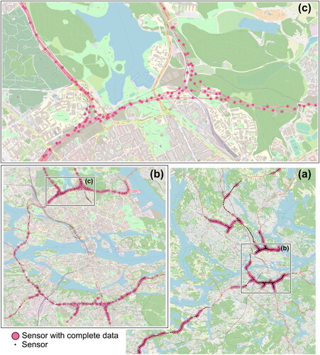
We consider the daytime period 05:00–21:30 and aggregate flow observations to 15-minute intervals (64 intervals). To avoid possible bias from missing, imputed, or erroneous observations on this study, we include only days and sensors that are active during all time intervals. In total, we have complete data for 499 sensors including 348 days during 2017 and 292 days during 2018. Year 2018 is split into a calibration dataset $X_C$ with 65 randomly selected working, weekend and holiday days, while the remaining 227 days, also a mix of all weekdays and holidays, are used as the evaluation dataset $X_E.$ Thus, the training dataset $X_T$ has 348 days. The size of each network-day vector is $M=64\cdot 499=31,936.$ This can be reduced by PCA dimensionality reduction to a dataset ${\overline{X}}_T$ with ${\overline{M}}_T=32.$ The reduced dataset ${\overline{X}}_T$ explains 90% of the variance with only 0.1% of the dimensions.

3.2. Clustering tendency

According to Adolfsson et al. (2019) it is good practice before clustering to evaluate the clustering tendency of dataset $X_T.$ For this we use the Hopkins statistics (for formulation see supplementary file S1), which is an independent index that does not require any particular clustering structure C. Values close to 0.5 indicate that the datasets are randomly distributed without natural clusters, indicating that clustering would be questionable, while values close to 1 represent well separated natural clusters. The metric is based on random sampling, and the average value from 150 repetitions is used here. The Hopkins statistic is 0.777 for dataset $X_T$ and 0.789 for the reduced dataset ${\overline{X}}_T.$ Thus, the values suggest the existence of natural clusters, and the data sets are good candidates for clustering methods to reveal representative day-types.

3.3. Computational experiments

The main objective of the computational experiments is to evaluate the clustering methods and representative day-types and test the common practice of internal evaluation. The data-driven clustering methods considered are k-means, agglomerative, ${\text{spectral}}_{\text{NN}},$ ${\text{spectral}}_{\text{CS}},$ ${\text{spectral}}_{\text{AMI}},$ p-median, and a-lex. Across all validation indices, the calendar-based clusterings are used as baseline to evaluate whether data-driven clustering reveal day-types that are not obvious, and thus assess the importance of data-driven methods. The calendar-based clusterings used in the experiments evaluation are summarized in Table 4.

Table 4. Internal evaluation indices for calendar-based clusterings.

Clustering C	|C|	Non-empty clusters
${\text{cal}}_{\text{dow}}$	7	7
${\text{cal}}_{\text{wkd}\times \text{hol}}$	8	7
${\text{cal}}_{\text{dow}\times \text{hol}}$	28	26

First, we explore and discuss the clustering results by calendar visualization. This visualization helps to analyze the day-type clusters and verifies if they match the expected patterns based on general knowledge of the traffic in the network during particular periods of the year. This visual tool does not enable evaluating minor differences but can be an easy check to filter out some clustering methods or to determine a reasonable number of clusters and their structure for the TMC. It also offers a tool for analyzing recognized day-types and their interpretation in terms of particular periods during the year as well as holidays. A similar approach has been used in Chiabaut and Faitout (2021); Toqué et al. (2017); Yang et al. (2017).

To quantify the quality of clustering to support the determination of the number of clusters, the clusterings are further evaluated using several internal and external clustering evaluation indices. Internal evaluation is based only on dataset $X_T$ and no external information is used. For external validation we use evaluation dataset $X_E$ and evaluate the short-term prediction performance for a 1-h horizon ($F=4$ future time intervals) for 56 time intervals between 06:00–20:30. The MAPE prediction performance metric is used as validation index. For the exponential smoothing the smoothing parameters ${\alpha }_j$ and past residuals ${\tilde{R}}_j$ are calibrated using the calibration dataset $X_T\cup X_C.$

4. Results

This section presents the results of the case study. First, we visualize the clusterings in the form of calendars and evaluate the differences among the data-driven and calendar-based clusterings. Next, the results of the internal evaluation are presented, followed by the outcome of the external evaluation based on short-term prediction is assessed, and comparison of the results. Finally, computational performance is discussed.

4.1. Calendar visualization

The three considered calendar-based clusterings are visualized in calendar form in Figure 3, while Figure 4 shows the data-driven clusterings for varying numbers of clusters. The days of the week are displayed on the y-axis, the calendar months on the x-axis and the colors indicate the clusters to which the days are classified. All data-driven methods capture to some extent expected clusters such as weekends and holidays. The ${\text{spectral}}_{\text{AMI}}$ method results in quite different clusters compared to the other methods. This is partially expected as the method does not use the absolute values in clustering but captures the dynamic of congestion in space-time. The ${\text{spectral}}_{\text{AMI}}$ method with seven or fewer clusters have only one cluster for weekdays and in general do not seem to establish a typical summer holiday cluster, which is the case for the other methods.

Figure 3. Calendar visualization of calendar-based clusterings for year 2017. White cells are days with missing data.

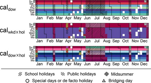
Figure 4. Calendar visualization of data-driven clustering methods clustered on original dataset $X_T.$ White cells are days with missing data.

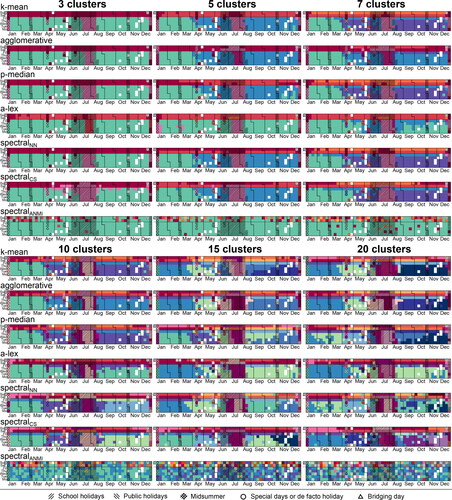
Apart from a-lex, the methods produce very similar clusters. With a-lex, small clusters are created for particularly distant days, while Mondays, Tuesdays and Wednesdays in autumn are placed in the same cluster as the spring months (see a-lex for 5, 7 and 10 clusters in Figure 4). ${\text{spectral}}_{\text{CS}}$ is the only method that places a mix of weekends (especially Saturdays) and summer holidays in one cluster for seven and fewer clusters. ${\text{Spectral}}_{\text{CS}}$ and ${\text{spectral}}_{\text{NN}}$ most clearly separate almost all Fridays into their own cluster, already with seven clusters. This occurs also for k-means, p-median and agglomerative with more than 15 clusters.

The most similar clusterings are produced by k-means and p-median, but the similarity decreases with the number of clusters. The p-median and ${\text{spectral}}_{\text{NN}}$ are the only clusterings that split January, February, and March into two large clusters. With 20 clusters, most clusterings are visually quite distinct from each other.

Figure 5 shows the spatio-temporal profiles of the revealed day-types. For this visualization we have selected two clustering methods with different objectives, p-median and a-lex, each with 10 clusters. Across all subplots in Figure 5 clusters are consistently labeled by number (1-10). Figure 5(a) visualizes the clusters in calendar form similar to Figure 4, to show seasonal and weekly similarities between the clustered days. Figure 5(b) shows network-wide day-type flow profiles as a function of the time of day. As expected, both clustering methods show clear differences between working day and weekend day-types, especially during the morning and afternoon peaks. Furthermore, the day-types are more diverse for weekdays during the holidays. Figure 5(c,d) extends the visualization of day-type time profiles to the spatial dimension on the y-axis. Flows are color-coded (low flows as dark blue and high flows as red) which enables the study of larger spatio-temporal differences in the network day-types.

Figure 5. Day-type centroids for p-median and a-lex with 10 clusters. (a) Calendar visualization (b) Aggregated network-wide day-time profiles. (c,d) Space-time matrices of flows across all sensors in the network and all considered time intervals. (c) for p-median and (d) for a-lex.

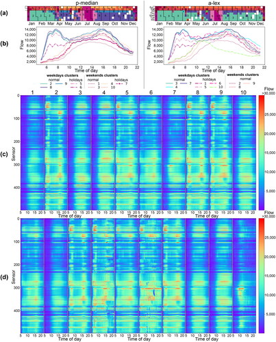
The main observations from Figure 5(c,d) are similar to Figure 5(b) in that for weekend day-types, the flows only increase from about 10:00, which is later than working day-types where the maximum flow is reached around 06:00-08:00. Additionally, Figure 5(c,d) reveal parts of the network that exhibit much higher traffic flows than elsewhere. For instance, cluster 2 with the p-median method, which represents typical weekdays in the winter months (January-March), shows a clear morning peak for sensors 30-50 and an afternoon peak for sensors 60-75. This pattern is also visible for clusters 5, 8 and 9. In contrast, clusters 3 and 4, representing weekends, show no such morning and afternoon peaks for these sensors.

An important difference between the two clustering methods is that a-lex results in three clusters (labeled 4, 6 and 10) of size one. These day vectors are considered very distant from the others. Cluster 10 is Mid-summer Day, which is one of the most important holidays in Sweden. Cluster 6 is the day before Mid-summer, which usually exhibits greatly increased traffic from the city to the countryside. We can see this increase in traffic compared to other working day-types especially in the middle of the day (see cluster 6 in Figure 5(b) and(d)). Note that there is a pattern of low flows revealed by Figure 5(d) in part of the network (sensors 300-350) around 15:00, which could be the result of severe congestion or an incident.

4.2. Internal evaluation results

In Figures 6–11 the calendar-based clusterings are used as reference lines. Note that all subplots showing the clustering performance on the reduced dataset ${\overline{X}}_T$ are evaluated on the complete space of the original dataset $X_T.$ Note also that the ${\text{spectral}}_{\text{AMI}}$ cannot be used with the reduced dataset ${\overline{X}}_T$ as it performs spatio-temporal clustering of observation entities at the day level.

Figure 6. Total within-cluster variance (TWCV) as a function of the number of clusters across clustering methods. (a) is the original dataset $X_T$ and (b) the reduced dataset ${\overline{X}}_T.$

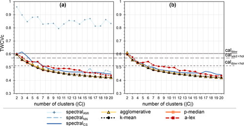
Figure 7. Total cluster dissimilarity (TCD) as a function of the number of clusters across clustering methods. (a) is the original dataset $X_T$ and (b) the reduced dataset ${\overline{X}}_T.$

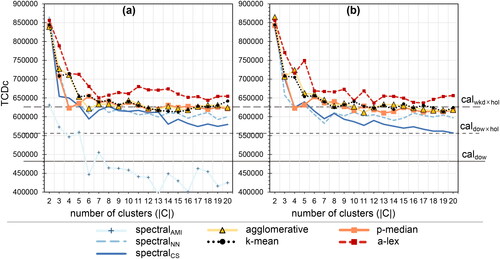
Figure 8. Silhouette score (SC) as a function of the number of clusters across clustering methods. (a) is the original dataset $X_T$ and (b) the reduced dataset ${\overline{X}}_T.$

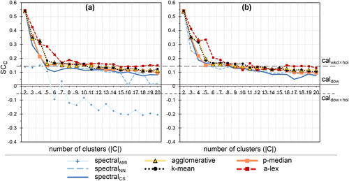
Figure 9. Davies-Bouldin (DB) index as a function of the number of clusters across clustering methods. (a) is the original dataset $X_T$ and (b) the reduced dataset ${\overline{X}}_T.$

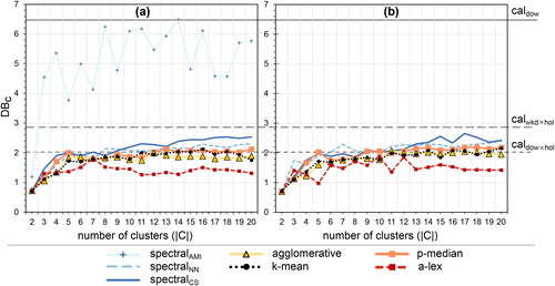
Figure 10. Short-term prediction performance external validation index as a function of the number of clusters across clustering methods. (a) is the original dataset $X_T$ and (b) the reduced dataset ${\overline{X}}_T.$

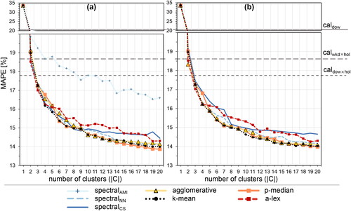
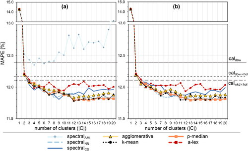
Figure 11. Exponential smoothing short-term prediction performance external validation index of the clustering C as a function of the number of clusters. (a) is the original dataset $X_T$ and (b) the reduced dataset ${\overline{X}}_T.$

It is expected that good clustering methods result in low within-cluster variance, decreasing with the number of clusters. Indeed, using TWCV as the measure of within-cluster variance in Figure 6 reveals a decreasing tendency with the number of clusters for all methods. However, the ${\text{spectral}}_{\text{AMI}}$ method provides poor results, about 30%-40% worse compared to the other methods. The a-lex method performs slightly worse in this aspect compared to the remaining methods, which is expected as it does not focus on within-cluster variance but optimizes the maximal distances in the dataset to its centroids. Note that the results for the reduced dataset in Figure 6(b) and the full dataset in Figure 6(a) are very similar for most methods.

Considering the performance based only on the TWCV index, the agglomerative, k-means, and p-median methods would be good choices with only minor differences among them.

Clustering is also expected to achieve high dissimilarity among clusters. Figure 7 shows TCD values for all methods and number of clusters. The TCD drops with a steep decrease with increased number of clusters until around three clusters, after which most methods are more or less stable with regard to the TCD value.

The ${\text{spectral}}_{\text{AMI}}$ method shows the poorest performance also here, while a-lex has the largest TCD value for any number of clusters, followed by agglomerative and k-means clustering. ${\text{Spectral}}_{\text{CS}}$ is the second worst performing method, especially on the reduced dataset ${\overline{X}}_T.$ Considering only TCD, the a-lex method would be the best performing method, especially for five clusters. Interestingly, for the original dataset, k-means has an increasing trend after 14 clusters. This behavior is not observed for the reduced dataset.

While TCD and TWCV usually are considered simultaneously to determine the best tradeoff between low within-cluster variance and high between-cluster distance, they often do not conclusively determine the best performing number of clusters to select. Some general conclusions can be drawn, however. ${\text{Spectral}}_{\text{AMI}}$ followed by ${\text{spectral}}_{\text{CS}}$ are clearly the worst performing clustering methods according to TCD and TWCV.

Silhouette score (SC, see Figure 8) is another commonly used validation index that considers the similarity both among days in the same cluster (cohesion) and to days in other clusters (separation). The higher the SC score, the better. However, we cannot see a clear maximum peak after two clusters, which means that selecting the best performing number of clusters across various clustering methods is not straightforward. Usually, a local maximum with reasonable SC is selected. A significant drop in SC stabilizes after 5 clusters for most methods. The a-lex method stabilizes at 7 clusters for the original dataset $X_T$ and 12 for the reduced dataset ${\overline{X}}_T.$ The a-lex method usually gets the highest SC score, which would mean it is a better clustering method. The separation aspect in SC overcomes the poorer cohesion (as reflected in TWCV). ${\text{Spectral}}_{\text{AMI}}$ and ${\text{Spectral}}_{\text{CS}}$ are performing the worst here as well.

The Davies-Bouldin (DB) index also accounts for cohesion and separation, but seeks the minimum peaks to determine the best clustering. According to this index, ${\text{spectral}}_{\text{AMI}}$ and ${\text{spectral}}_{\text{CS}}$ are again the worst performing and a-lex the best performing method (see Figure 9). Meanwhile, the most appropriate number of clusters is difficult to determine.

In Table 5, we summarize our selection of number of clusters per method, omitting ${\text{spectral}}_{\text{AMI}}$ because of its poor performance. Although we provide two values for most of methods, the final choice would in most cases be the smaller value (higlighted by ”bold” style in the table) unless there is additional evidence available.

Table 5. Best performing number of clusters according to considered internal indices per clustering method. The clusterings considered as best and reasonable are highlighted in bold.

Clustering method	TWCV& TCD	SC	DB	all in consideration
${\text{spectral}}_{\text{NN}}$	5,7	7	7	7
${\text{spectral}}_{\text{CS}}$	4,8	8	6,8	8
agglomerative	4,7	4,6	6,11	4,6
k-means	4,6	4, 7	6, 10	4,6
p-median	6,10	7,11	6, 11	6,11
a-lex	5,11	5, 8	4, 11	5,11

To conclude, none of the internal indices in our case study clearly point to a single best natural clustering. Across all internal validation indices, agglomerative and k-means seems to be the most robust method when it comes to clustering of the original and the reduced dataset evaluated in the original dataset space, followed by p-median clustering. The a-lex method results in clusterings with expected characteristics such as larger cluster disimilarity (TCD). In contrast, it therefore also performs worse than other methods when it comes to within-cluster variance (TWCD). P-median has similar performance as agglomerative and k-means heuristics across all internal evaluation indices. Concerning dimensionality reduction, the considered clustering methods seem to result in clustering with similar performance in internal evaluation.

4.3. Short-term prediction performance

In this section we consider external validation criteria represented here by the performance in application. We investigate the performance of the clustering methods on two short-term prediction models. First, we evaluate on a basic prediction scheme using the day-type centroid vector defined as the historical mean vector (Eq. 5(5) $${\widehat{v}}_{if}^{x_d}:=v_{if}^{\overline{y}}, i=1,\dots ,I;f=j,\dots ,j+F$$(5) ). The second prediction scheme extends the basic prediction scheme by using exponential smoothing for the short-term prediction (Eq. 7(7) $${\widehat{v}}_{if}^{x_d}:=v_{if}^{\overline{y}}+\sum _{k=0}^{{\tilde{R}}_j}(v_{i,j-k}^{x_d}-v_{i,j-k}^{\overline{y}}){\alpha }_j^{f-j+k}, i=1,\dots ,I;f=j,\dots ,j+F$$(7) ). The focus is on the selection of day-type clusters and not on the optimization of the clustering-based prediction model for its best performance.

Figure 10 shows the performance of the basic prediction scheme in terms of MAPE (see Eq. 6(6) $$\text{MAPE}=\frac{1}{J}\sum _{j=1}^J\frac{1}{N_E}\sum _{d=1}^{N_E}\frac{1}{I}\sum _{i=1}^I\frac{1}{F}\sum _{f=1}^{\min \{F,J-j\}}\frac{|v_{i,j+f}^{x_d}-{\widehat{v}}_{i,j+f}^{x_d}|}{v_{i,j+f}^{x_d}}$$(6) ). There is a clear decreasing tendency with the number of clusters. On the one hand, the a-lex clustering method, with good internal validation, perform worse than the other methods on both the original $X_T$ (see Figure 10(a)) and reduced dataset ${\overline{X}}_T$ (see Figure 10(b)), systematically. On the other hand, the p-median, k-mean, and agglomerative methods with lower internal evaluation ranking perform best and display similar performance on the original dataset $X_T$ and the reduced dataset ${\overline{X}}_T.$ Note that MAPE continues to decrease with an increased number of clusters beyond the optimal number of clusters (4–11) indicated by the internal validation criteria. In addition, all methods outperform the calendar-based methods for three or more clusters.

Already three data-driven clusters can outperform 28 calendar-based clusters of ${\text{cal}}_{\text{dow}\times \text{hol}}$ (see Figure 10). Using 14 data-driven clusters improves prediction accuracy by almost 4% overall.

The improvement in MAPE with increasing number of clusters flattens for the original $X_T$ and reduced dataset ${\overline{X}}_T$ at around 19 and 17 clusters, respectively. Only a-lex gets a more intense improvement with 19 clusters on both the original and reduced datasets. Thus, considering this external validation index, the most appropriate number of clusters would be significantly higher than the number indicated by internal validation. Note that all methods, including ${\text{spectral}}_{\text{AMI}}$ clustering, outperform calendar-based clusterings.

In Figure 11 the results for the exponential smoothing prediction scheme are presented. In general, exponential smoothing yields a significant improvement in prediction error of about 2-3 percentage points, compared to the basic scheme.

In general, compared to the basic prediction scheme, the exponential smoothing uses more within-day information. As shown in Figure 10, all methods (except for ${\text{spectral}}_{\text{AMI}}$) outperform the calendar-based methods. However, for both the original $X_T$ and the reduced dataset ${\overline{X}}_T,$ the performance does not improve beyond around 12 clusters, unlike the case with the basic prediction scheme. This may indicate that the value of larger numbers of clusters decreases when more intra-day information is used. Same as for historical mean prediction scheme, three data-driven clusters can provide a much better basis for prediction models than 28 calendar-based clusters (${\text{cal}}_{\text{dow}\times \text{hol}}$). Considering this validation index, a reasonable number of clusters to choose would be in the range 4-12 depending on the clustering method.

The results for both prediction schemes highlight the applicability and benefits of using day clustering (calendar-based or data-driven) before training and calibrating prediction models.

4.4. Final evaluation of the clusterings

Considering clustering based on the original dataset $X_T,$ 9 clusters would be a reasonable tradeoff between prediction performance and internal evaluation selection for ${\text{spectral}}_{\text{CS}}$ and a-lex. Selecting 4 clusters for a-lex would lead to a loss of 1% MAPE under the basic prediction scheme responsible. However, under the scheme with exponential smoothing, 4 or 9 clusters gives about the same performance. The 5 and 11 clusters for a-lex suggested by DB and TCD, respectively, have significant drops in performance considering both prediction schemes. Thus, 9 clusters has the most robust combination of prediction performance and performance according to SC and DB.

For k-means, agglomerative, p-median, ${\text{spectral}}_{\text{NN}}$ there is no clear selection with the basic prediction scheme, while exponential smoothing clearly points to 12 clusters and to 8 clusters for ${\text{spectral}}_{\text{NN}}.$ The selection based on internal evaluation would choose half or less of day-types and underestimate the number of clusters. Hence, the full potential of day clustering would not be utilized for this application.

The final selection of the number of representative day-types for our case study would be: ${\text{spectral}}_{\text{NN}}:$ 8, ${\text{spectral}}_{\text{CS}}:$ 9, agglomerative: 12, k-means: 12, p-median: 12, and a-lex: 9. If the dimensionally reduced dataset ${\overline{X}}_T$ is used the choice would be 12 clusters for all the considered clustering methods, including a-lex.

4.5. Computational performance

Table 6 summarizes the computational costs (time) for the considered clustering methods. The cost includes the clustering itself, and in methods such as ${\text{spectral}}_{\text{AMI}},$ ${\text{spectral}}_{\text{CS}},$ p-median and a-lex also the calculation time for pre-computing the similarity or distance matrix before clustering. As highlighted in (Cebecauer et al., 2019) the calibration of ${\text{spectral}}_{\text{AMI}}$ could be computationally very expensive, even though the spectral clustering itself is fast. As expected, p-median and a-lex take significantly longer than the other clustering methods. On the original dataset $X_T,$ the ${\text{spectral}}_{\text{NN}}$ is the most efficient considering computational time, however it is outperformed by agglomerative and k-means on the reduced dataset ${\overline{X}}_T.$

Table 6. Total computational time for clustering methods to run 19 clusterings with 2-20 clusters.

	Computational time [s]
Clustering method	Original dataset $X_T$	Reduced dataset ${\overline{X}}_T$
${\text{spectral}}_{\text{AMI}}$	42,135.54	–
${\text{spectral}}_{\text{NN}}$	12.52	8.74
${\text{spectral}}_{\text{CS}}$	239.87	271.16
Agglomerative	85.00	4.92
k-means	202.50	7.80
p-median	3,203.00	292.95
a-lex	4,130.93	1391.82

Another important observation is that dimensionality reduction has the potential to significantly lower the computational costs, by over 20 times for k-means and agglomerative (which do not use a pre-computed distance matrix) and more than 10 times for p-median. Conversely, the ${\text{spectral}}_{\text{CS}}$ method shows a slight increase in computational time. There are two main drivers that lead to lower computational times for the reduced dataset. First, the calculation of distances or similarities needs only to consider 0.1% of the original dataset dimensions. Second, the natural coordinate system of the reduced dataset may provide better clustering tendency, of which clustering methods can take advantage. The algorithms used for p-median and a-lex consider unique allocation distances, which could likely be lowered for the reduced dataset ${\overline{X}}_T$ and thus directly affect the computational performance.

${\text{Spectral}}_{\text{AMI}}$ is included in the paper as it is one of few methods used for network-wide day clustering in the transport literature with application to short-term prediction (Lopez et al., 2017). However, throughout this paper, it performs poorly on both internal and external validation, as well as in terms of computational costs. This is corroborated by Cebecauer et al. (2019), where it was shown that the proper calibration for this method to short-term prediction application can be computationally very expensive. In addition, it was shown in Cebecauer et al. (2019) that ${\text{spectral}}_{\text{AMI}}$ is usually outperformed by ${\text{spectral}}_{\text{CS}},$ which is consistent with our findings.

In general, the computational costs for the methods show large differences, indicating that agglomerative and k-means may be the most scalable methods for larger applications, especially for the reduced dataset, for which prediction performance is almost identical to the original dataset at a fraction of the cost.

When using the exponential smoothing prediction scheme, additional calibration of the exponential smoothing parameters ${\alpha }_j$ for each time interval j and number of clusters (from 2 to 20), takes about 16-20 h for each method.

5. Discussion

We first discuss the clustering quality of the clustering methods using various internal validation metrics such as Total within-cluster variance (TWCV), Total Cluster Dissimilarity (TCD), Silhoute Score (SC) and Davies-Bouldin (DB) index. The selected number of clusters strongly depends on the chosen metric but generally falls in the range of 4 to 11 clusters. Across all internal validation indices, k-means seems to be the most robust method on both the original and the reduced dataset, followed by p-median and agglomerative clustering. The a-lex method results in clusterings with expected characteristics such as larger cluster disimilarity (TCD) and worse within-cluster variance (TWCD). The ${\text{spectral}}_{\text{CS}}$ and ${\text{spectral}}_{\text{AMI}}$ method perform worst across validation indices.

For the external validation, our first finding using the basic prediction scheme is that the selected number of clusters according to internal evaluation criteria (4-11 clusters), would have severely underestimated the number of clusters needed for the best prediction performance, which would have resulted in a loss of prediction accuracy by up to 20%. Across all methods, the optimal number of clusters for prediction would be in the range of 17-20 clusters. The best performing methods in short-term prediction are p-median, k-means and agglomerative clustering with similar performance on both the reduced and original dataset (MAPE around 14%). Note that all methods outperform the calendar-based methods for this scheme.

For the exponential smoothing prediction scheme, the required number of clusters varies between 7 and 13, depending on the clustering method, indicating that prediction schemes that incorporate more intra-day information may need fewer clusters. Here k-means, p-median, agglomerative and ${\text{spectral}}_{\text{NN}}$ are the best performing methods with very similar MAPE scores (around 11.8%) for both the original and the reduced dataset. Furthermore, the difference in performance between data-driven and calendar-based clusterings is significantly reduced.

The exponential smoothing scheme, which uses intra-day correlations, requires additional computational time for calibrating smoothing parameters (up to 20 h for each clustering method) and results in a smaller number of clusters. Conversely, the basic historical mean scheme results in a larger number of clusters but requires no calibration effort at all after clustering, greatly reducing the computational burden. This can make a basic scheme a good proxy for external evaluation instead of using a more sophisticated prediction model. However, a larger number of clusters from which simpler methods can benefit, could lead to overfitting for more complex prediction models, resulting in reduced prediction performance on new data. We therefore recommend the combination of internal and external indices to select the appropriate number of clusters and find the best tradeoff. Note that in our data the risk of overfitting seems to be limited, as (for example) the prediction accuracy (on unseen data) with p-median clustering for the exponential smoothing model with 20 clusters instead of 12 leads to an accuracy loss of only about 0.002%. On the other hand, if only 6 or 7 day-types are selected with internal evaluation, the loss in performance is significantly higher.

6. Conclusions

This paper compares external evaluation, through the application of short-term prediction, with the common practice of using internal clustering evaluation methods for revealing representative network-wide day-types. We have compared commonly used clustering methods including k-means, hierarchical agglomerative and spectral clustering with location-allocation problems, based on well-defined objectives and algorithms. Furthermore, these data-driven clustering methods are compared to calendar-based clusterings. Data-driven clustering reveals representative day-types more effectively than calendar-based methods across all internal and external validation indices, with significantly fewer clusters.

Importantly, our work confirms that internal evaluation isolated from the application may underestimate the number of clusters needed in the application and thus may fail to achieve the full potential of day clustering for such applications. Furthermore, different internal evaluation indices lead to different results. Combining internal and external evaluation shows significant improvement in prediction performance, while still avoiding overfitting to training data. Our work further shows that dimensionality reduction may reduce computational cost by up to 20 times, using just 0,1% of the original dataset dimensions, without significantly reducing clustering and prediction performance. This makes the technique a good candidate for larger case studies with hundreds of thousands of dimensions.

While the best performing clustering methods give similar prediction accuracy, their computational costs vary largely for both reduced and original datasets, indicating that k-means and agglomerative clustering may be the most scalable methods.

The prediction methods used for external validation are relatively simple. However, our results confirm that clustering improves the prediction performance as suggested in Laña et al. (2021). This work shows that a combination of internal criteria and external validation could provide more robust performance in the application and better utilizes the potential of day-types. Note that input from experts with knowledge of local traffic patterns can still be of high value, especially if the application is complex to model for external evaluation.

Day-type clusters have a high potential for many traffic management center (TMC) applications. Data-driven day-types, in contrast to pure calendar-based classifications, can improve knowledge about daily traffic patterns and be a key ingredient in incident handling and scenario-based traffic management. Cluster-based prediction models can represent more robust baselines in daily operations when no traffic model is needed or calibrated for advanced simulation-based predictions. In addition, our results indicate that these day-type clusters provide more homogeneous datasets, making the calibration and performance of more complex methods more robust. We have shown that by considering the exponential smoothing prediction model example. So far, day clustering has only been associated with naive prediction models Chiabaut and Faitout (2021); Chrobok et al. (2004); Krishnakumari et al. (2020); Lopez et al. (2017); Van Hinsbergen et al. (2007); Wild (1997), and this is one step ahead.

In this work we identify several limitations. The data for the case study concerns only motorways, around Stockholm, Sweden. Future work should extend the analysis in order to validate the results for more general networks and locations. We consider two years of traffic data in this study (500 sensors, 15 min time intervals). In literature, at least two years of data, when the first year is used for training and second for evaluation, is considered sufficient (Manibardo et al., 2021). Future work could extend this time period to be able to more reliably catch seasonality effects, although too large time-spans may suffer from significant infrastructure changes and evolution in traffic demand patterns.

In addition to the clustering methods and internal metrics considered in this work, there exist many others that have not been considered. In this work, the focus is on internal validation when determining the number of clusters. Thus, some other classic clustering algorithms, such as affinity propagation, DBSCAN, and density peak clustering, are not considered. Future work may consider these algorithms for revealing representative day-types, as they do not require the number of clusters to be specified.

Future work should also investigate tradeoffs between network-wide and local day clustering. According to Cebecauer et al. (2018), clustering of spatio-temporal “neighborhoods” of similar observation entities may result in more robust and accurate predictions. Thus, future work could combine day-type clustering with spatio-temporal clustering of observation entities to enhance short-term traffic prediction further. Furthermore, more sophisticated distance or similarity measures than Euclidean distance may be used to potentially improve the resulting prediction performance. Considering that in real-world applications, not all data from sensors in the network may be available at all times, it would be relevant to explore the impact of missing and noisy data on the presented methodology. Finally, future work may focus on combining the strengths of calendar-based and machine-learning classification models, enabling the use of these clusters not only for short-term prediction applications but also for prediction over longer periods. It may also be useful to evaluate the similarity of representative day-types recognized by different traffic attributes such as speed and flows.

Author contributions

M. Cebecauer: Conceptualization, Methodology, Data processing, Software, Results interpretation, Visualization, Writing—original draft. E. Jenelius: Conceptualization, Supervision, Results interpretation, Writing—reviewing and editing, Funding Acquisition. D. Gundlegård: Conceptualization, Methodology, Data collection and processing, Results interpretation, Writing—reviewing and editing, Funding Acquisition. W. Burghout: Conceptualization, Results interpretation, Writing—reviewing and editing, Funding Acquisition.

Acknowledgement

The authors would like to thank Tomas Julner and Per-Olof Svensk at the Swedish Transport Administration for their support and provision of the data.

Disclosure statement

No potential conflict of interest was reported by the authors.

Additional information

Funding

The work was funded in part by the Swedish Transport Administration through the POST and POST2 projects (Prediction and Scenario-Based Traffic Management), MMTL (Multimodal traffic management) and TRENoP Strategic Research Area.

References

- Adolfsson, A., Ackerman, M. and Brownstein, N. C. (2019). To cluster, or not to cluster: An analysis of clusterability methods. Pattern Recognition, 88, 13–26. https://doi.org/10.1016/j.patcog.2018.10.026
- Buzna, L., Koháni, M. and Janáček, J. (2014). An approximation algorithm for the facility location problem with lexicographic minimax objective. Journal of Applied Mathematics, 2014, 1–12. https://doi.org/10.1155/2014/562373
- Cebecauer, M., Gundlegård, D., Jenelius, E. and Burghout, W. (2019). 3d speed maps and mean observations vectors for short-term urban traffic prediction. In Transportation Research Board Annual Meeting (TRB) (pp. 1–20).
- Cebecauer, M., Jenelius, E. and Burghout, W. (2017). Integrated framework for real-time urban network travel time prediction on sparse probe data. IET Intelligent Transport Systems, 12(1), 66–74. https://doi.org/10.1049/iet-its.2017.0113
- Cebecauer, M., Jenelius, E. and Burghout, W. (2018). Spatio-temporal partitioning of large urban networks for travel time prediction. In 2018 21st International Conference on Intelligent Transportation Systems (ITSC) (pp. 1390–1395). https://doi.org/10.1109/ITSC.2018.8569648
- Chiabaut, N. and Faitout, R. (2021). Traffic congestion and travel time prediction based on historical congestion maps and identification of consensual days. Transportation Research Part C: Emerging Technologies, 124, 102920. https://doi.org/10.1016/j.trc.2020.102920
- Chrobok, R., Kaumann, O., Wahle, J. and Schreckenberg, M. (2004). Different methods of traffic forecast based on real data. European Journal of Operational Research, 155(3), 558–568. https://doi.org/10.1016/j.ejor.2003.08.005
- Clark, S. (2003). Traffic prediction using multivariate nonparametric regression. Journal of transportation engineering, 129(2), 161–168. https://doi.org/10.1061/(ASCE)0733-947X(2003)129:2(161)
- Davies, D. L. and Bouldin, D. W. (1979). A cluster separation measure. IEEE transactions on pattern analysis and machine intelligence 2 224–227. https://doi.org/10.1109/TPAMI.1979.4766909
- Djukic, T., Van Lint, J. and Hoogendoorn, S. (2012). Application of principal component analysis to predict dynamic origin–destination matrices. Transportation research record, 2283(1), 81–89. https://doi.org/10.3141/2283-09
- Ester, M., Kriegel, H.-P., Sander, J. and Xu, X. (1996). A density-based algorithm for discovering clusters in large spatial databases with noise. In KDD-96 Proceedings (pp. 226–231).
- Estivill-Castro, V. (2002). Why so many clustering algorithms: A position paper. ACM SIGKDD Explorations Newsletter, 4(1), 65–75. https://doi.org/10.1145/568574.568575
- Feldman, R., Sanger, J. (2007). The text mining handbook: Advanced approaches in analyzing unstructured data. Cambridge University Press.
- Ferranti, F. (2020). Public transport origin-destination matrices: Pattern recognition and short-term prediction. KTH Royal institute of technology.
- Frey, B. J. and Dueck, D. (2007). Clustering by passing messages between data points. Science, 315(5814), 972–976. https://doi.org/10.1126/science.1136800
- García, S., Labbé, M. and Marín, A. (2011). Solving large p-median problems with a radius formulation. INFORMS Journal on Computing, 23(4), 546–556. https://doi.org/10.1287/ijoc.1100.0418
- Jenelius, E. and Koutsopoulos, H. N. (2018). Urban network travel time prediction based on a probabilistic principal component analysis model of probe data. IEEE Transactions on Intelligent Transportation Systems, 19(2), 436–445. https://doi.org/10.1109/TITS.2017.2703652
- Ji, Y. and Geroliminis, N. (2012). On the spatial partitioning of urban transportation networks. Transportation Research Part B: Methodological, 46(10), 1639–1656. https://doi.org/10.1016/j.trb.2012.08.005
- Krishnakumari, P., Cats, O. and van Lint, H. (2020). A compact and scalable representation of network traffic dynamics using shapes and its applications. Transportation Research Part C: Emerging Technologies, 121, 102850. https://doi.org/10.1016/j.trc.2020.102850
- Kumar, S. V. and Vanajakshi, L. (2015). Short-term traffic flow prediction using seasonal arima model with limited input data. European Transport Research Review, 7(3), 1–9. https://doi.org/10.1007/s12544-015-0170-8
- Laña, I., Sanchez-Medina, J. J., Vlahogianni, E. I. and Del Ser, J. (2021). From data to actions in intelligent transportation systems: A prescription of functional requirements for model actionability. Sensors, 21(4), 1121. https://doi.org/10.3390/s21041121
- Lloyd, S. (1982). Least squares quantization in pcm. IEEE Transactions on Information Theory, 28(2), 129–137. https://doi.org/10.1109/TIT.1982.1056489
- Lopez, C., Leclercq, L., Krishnakumari, P., Chiabaut, N. and Lint, H. (2017). Revealing the day-to-day regularity of urban congestion patterns with 3d speed maps. Scientific Reports, 7(1), 14029. https://doi.org/10.1038/s41598-017-14237-8
- Luo, D., Cats, O. and Van Lint, H. (2017). Analysis of network-wide transit passenger flows based on principal component analysis. In 2017 5th IEEE International Conference on Models and Technologies for Intelligent Transportation Systems (MT-ITS) (pp. 744–749). https://doi.org/10.1109/MTITS.2017.8005611
- MacQueen, J., et al. (1967). Some methods for classification and analysis of multivariate observations. In Proceedings of the Fifth Berkeley Symposium on Mathematical Statistics and Probability (Vol. 1, pp. 281–297).
- Manibardo, E. L., Laña, I. and Del Ser, J. (2021). Deep learning for road traffic forecasting: Does it make a difference? IEEE Transactions on Intelligent Transportation Systems, 23(7), 6164–6188. https://doi.org/10.1109/TITS.2021.3083957
- Murtagh, F. (1983). A survey of recent advances in hierarchical clustering algorithms. The Computer Journal, 26(4), 354–359. https://doi.org/10.1093/comjnl/26.4.354
- Patel, M., Valderrama, C. and Yadav, A. (2022). Metaheuristic enabled deep convolutional neural network for traffic flow prediction: Impact of improved lion algorithm. Journal of Intelligent Transportation Systems, 26(6), 730–745. https://doi.org/10.1080/15472450.2021.1974857
- Pfitzner, D., Leibbrandt, R. and Powers, D. (2009). Characterization and evaluation of similarity measures for pairs of clusterings. Knowledge and Information Systems, 19(3), 361–394. https://doi.org/10.1007/s10115-008-0150-6
- Rendón, E., Abundez, I., Arizmendi, A. and Quiroz, E. M. (2011). Internal versus external cluster validation indexes. International Journal of computers and communications, 5(1), 27–34.
- Rousseeuw, P. J. (1987). Silhouettes: A graphical aid to the interpretation and validation of cluster analysis. Journal of Computational and Applied Mathematics, 20, 53–65. https://doi.org/10.1016/0377-0427(87)90125-7
- Saeedmanesh, M. and Geroliminis, N. (2016). Clustering of heterogeneous networks with directional flows based on “snake” similarities. Transportation Research Part B: Methodological, 91, 250–269. https://doi.org/10.1016/j.trb.2016.05.008
- Shi, J. and Malik, J. (2000). Normalized cuts and image segmentation. IEEE Transactions on Pattern Analysis and Machine Intelligence, 22(8), 888–905. https://doi.org/10.1109/34.868688
- Toqué, F., Côme, E., El Mahrsi, M. K. and Oukhellou, L. (2016). Forecasting dynamic public transport origin-destination matrices with long-short term memory recurrent neural networks. In 2016 IEEE 19th international conference on intelligent transportation systems (ITSC) (pp. 1071–1076). https://doi.org/10.1109/ITSC.2016.7795689
- Toqué, F., Khouadjia, M., Come, E., Trepanier, M. and Oukhellou, L. (2017). Short & long term forecasting of multimodal transport passenger flows with machine learning methods. In 2017 IEEE 20th International Conference on Intelligent Transportation Systems (ITSC) (pp. 560–566). https://doi.org/10.1109/ITSC.2017.8317939
- Van Hinsbergen, C., Van Lint, J. and Sanders, F. (2007). Short term traffic prediction models. In Proceedings of the 14th World Congress on Intelligent Transport Systems (ITS), Held Beijing, October 2007.
- van Lint, J. W. C. and van Hinsbergen, C. P. I. J. (2012). Short-term traffic and travel time prediction models. Artificial Intelligence Applications to Critical Transportation Issues, 22, 22–41.
- Vlahogianni, E. I., Karlaftis, M. G. and Golias, J. C. (2014). Short-term traffic forecasting: Where we are and where we’re going. Transportation Research Part C: Emerging Technologies, 43, 3–19. https://doi.org/10.1016/j.trc.2014.01.005
- Ward Jr, J. H. (1963). Hierarchical grouping to optimize an objective function. Journal of the American statistical association, 58(301), 236–244. https://doi.org/10.1080/01621459.1963.10500845
- Weijermars, W. and Van Berkum, E. (2005). Analyzing highway flow patterns using cluster analysis. In Proceedings. 2005 IEEE Intelligent Transportation Systems, 2005 (pp. 308–313). https://doi.org/10.1109/ITSC.2005.1520157
- Weijermars, W. A. M. (2007). Analysis of urban traffic patterns using clustering Analysis of urban traffic patterns using clustering (Vol. 41). Netherlands TRAIL Research School.
- Wild, D. (1997). Short-term forecasting based on a transformation and classification of traffic volume time series. International Journal of Forecasting, 13(1), 63–72. https://doi.org/10.1016/S0169-2070(96)00701-7
- Yang, C., Yan, F. and Xu, X. (2017). Daily metro origin-destination pattern recognition using dimensionality reduction and clustering methods. In 2017 IEEE 20th International Conference on Intelligent Transportation Systems (ITSC) (pp. 548–553). https://doi.org/10.1109/ITSC.2017.8317899
- Zhang, J., Che, H., Chen, F., Ma, W. and He, Z. (2021). Short-term origin-destination demand prediction in urban rail transit systems: A channel-wise attentive split-convolutional neural network method. Transportation Research Part C: Emerging Technologies, 124, 102928. https://doi.org/10.1016/j.trc.2020.102928
- Zhang, J., Wang, F.-Y., Wang, K., Lin, W.-H., Xu, X. and Chen, C. (2011). Data-driven intelligent transportation systems: A survey. IEEE Transactions on Intelligent Transportation Systems, 12(4), 1624–1639. https://doi.org/10.1109/TITS.2011.2158001
- Zhu, L., Yu, F. R., Wang, Y., Ning, B. and Tang, T. (2018). Big data analytics in intelligent transportation systems: A survey. IEEE Transactions on Intelligent Transportation Systems, 20(1), 383–398. https://doi.org/10.1109/TITS.2018.2815678