A platoon formation algorithm for intersections with blue phase control in mixed traffic

Abstract

Increasing attention is being paid to intersection signal control with cooperative platoons. Assuming platoons being formed, such platoons cannot only improve the intersection capacity but also minimize the number of control units, especially when dedicated connected and automated vehicle (CAV) lanes are considered. However, the platoon formation process is often neglected, especially for lane-changing and overtaking maneuvers in mixed traffic. This may jeopardize the potential of signal control with platoons. This article proposes a platoon formation algorithm that computes the optimal lane, platoon sequence, and speed profiles of CAVs under the requirement of the central traffic controller. The algorithm is designed for mixed traffic conditions and hence the performance of human-driven vehicles is also considered. A mixed integer linear program model is formulated to minimize the deviation from the desired platoon configuration and the disturbance to overall traffic under any arbitrary initial condition. Numerical experiments are designed to test the effectiveness and the computational performance of the proposed algorithm. Results show that CAVs with signal control can form platoons with rational motion. Besides, the platoon penetration significantly affects platooning feasibility, while the platoon length does not. This suggests that CAVs can form long platoons at intersections to improve traffic throughput.

Keywords:

• blue phase
• connected and automated vehicle
• mixed traffic
• platoon formation
• signalized isolated intersection

1. Introduction

Intersections are main bottlenecks in urban road networks. The competition of rights of way from different movement directions deems signal control at intersections necessary since signal control can ensure multi-modal safety and improve efficiency at high traffic demands. Traffic signal control at intersections has been widely studied. Since Webster (1958) proposed the stage-based control approach, a number of methods have been proposed, including fixed-time control (Little et al., 1981), vehicle-actuated control (G. Zhang & Wang, 2010), and adaptive control (Memoli et al., 2017; Mohajerpoor et al., 2019).

The advancement of connected and automated vehicle (CAV) systems can induce drastic changes in the architecture of traffic control systems. For instance, Varaiya (1993) developed a control system with different layers, i.e., physical, regulation, planning or coordination, link, and network layers from the bottom. Baskar et al. (2011) extended this architecture by adding a subnetwork layer between the network and link layers. The physical, regulation, and coordination layers are located at the vehicle system, while the link and network layers are located at roadside or traffic control centers.

Considerable attention has been devoted to platoon regulation layer and physical layer with CAVs on highways due to the benefits of increased roadway capacity and traffic flow stability (Schakel et al., 2010). In urban network, flow stability is less relevant and the interaction between traffic control and CAV platoons becomes a necessity for platoon operations. Normally such platoons are assumed to be formed when entering the studied network/intersection, which ignores the essential process of platoon reformation. However, this becomes nontrivial when dedicated CAV lanes and dedicated signal phase (blue phase) are considered and designed; the platoon formation can lead to mandatory lane changes and platoon reconfiguration in mixed traffic flow, where the behaviors of conventional vehicles have to be considered. The focus on this research is therefore on the platoon configuration problem at signalized intersections, which determines the platoon size (i.e., the platoon length) and order of platoon members in mixed traffic to match the targets set by the traffic control layer while reducing disturbance to conventional vehicles. It essentially deals with the problem at the platoon coordination/management layer and we use the terms platoon coordination and platoon management interchangeably in the article.

To justify the contribution of our article, we first review the studies at the platoon regulation layer and then move to the platoon management layer.

1.1. Platoon regulation at signalized intersections

CAVs can provide more timely and accurate information to traffic signal control systems and better actuation of the control signals. There are in general five categories in this field. Studies in the first category use trajectory information from CAVs to acquire a better estimate of current traffic state and to schedule optimal signal timing plans (Guler et al., 2014; Rakha et al., 2011). The second category optimizes the trajectories of CAVs according to the known signal phase and timing (SPaT) information, leading to environment-friendly and efficient operation of CAVs (Huang & Peng, 2017; Jiang et al., 2006; Rakha et al., 2012). The third category combines the first and the second categories and optimizes the signal timing and trajectories of CAVs at the same time (Guo et al., 2019; Jiang et al., 2006; Z. Li et al., 2014; Yu et al., 2018). This category utilizes both the situation awareness and the cooperative maneuvering potential of CAVs, resulting in further improvements in traffic control performance. In the case of a fully CAV environment, the fourth category, named signal-free control, directly controls CAV trajectories without the need of different signal phases. The difference between the third category and the fourth category is the presence/absence of control signal (Dresner & Stone, 2004; Lee & Park, 2012; L. Li & Wang, 2006; Z. Li et al., 2014; Yu et al., 2019). Although signal-free control is a drastic change in traffic control and may lead to high efficiency, it seriously limits its application in practice since it excludes vulnerable road users and cannot function in mixed traffic. Recently, a fifth category method that combines the signal-free control and signal control by setting a CAV-only signal phase, i.e., the blue phase, was proposed (Rey & Levin, 2019). The idea is that CAVs can pass the intersection with conflicting movements similar to a signal-free manner in the blue phase, while in other phases they follow the traditional signal control design. However, in existing blue phase control studies, vehicle arrivals are considered as exogenous input and are not optimized. Platoons are assumed formed under the initial condition and the platoon management is therefore ignored.

1.2. Platoon management layer

The platoon management layer can coordinate CAV maneuvers to actively form/merge/split platoons to increase efficiency at intersections (P. Wang et al., 2020). Moreover, with the control unit changing from individual vehicles to platoons, the complexity of traffic control algorithms can be reduced. Moreover, with the control unit changing from individual vehicles to platoons, the complexity of traffic control algorithms can be reduced. When vehicles travel in platoons, they can closely follow and respond to the actions of the lead vehicle in a coordinated manner. This platooning behavior can be achieved through communication and coordination among vehicles, eliminating the need for individual control of each vehicle. Therefore, once a platoon is formed, the entire platoon can be considered as a single control unit, reducing the number of control units from the number of vehicles to the number of platoons.

Considerable efforts have been devoted to platoon coordination on highway networks, controlling or scheduling CAVs in a decentralized or centralized manner to actively form platoons. Decentralized platoon management is mainly based on rules for leader selection and member affiliation (Cooper et al., 2016), where member affiliation refers to the rule of whether and how the member joins a platoon. Most of the decentralized rules are passive clustering in an ad hoc way within a communication range. On the contrary, centralized platoon management is usually related to an optimization problem, where the optimization objectives normally have multiple terms. These objectives include maximizing platoon size or forming platoons in suitable sizes (Hall & Chin, 2005), maximizing the lifetime (Hall & Chin, 2005), minimizing platoon formation time (Y. Zhang & Cao, 2011), and minimizing fuel consumption (Luo et al., 2018).

Compared with platoon management at highway, studies of platoon management at signalized intersection are still scarce (Bashiri & Fleming, 2017; He et al., 2012; Jiang et al., 2006; Liu et al., 2019). Many studies take formed platoons as granted in the initial conditions (Du et al., 2016) while few studies consider the platoon formation process at intersections. Similarly to highways, in Qiu et al. (2013), an ad hoc way of platoon formation based on communication range is reported. In a signal timing-based approach (Faraj et al., 2017), vehicles merge to the front platoon if they can pass the intersection during the green phase. Tallapragada and Cortés (2019) and Z. Wang et al. (2018) proposed clustering-based platoon formation methods with a pre-defined platoon length. Tallapragada and Cortés (2019) used the K-means cluster algorithm to adjust the platoon size according to the requirement of the traffic control center. Z. Wang et al. (2018) proposed a cluster-wise cooperative management method, where the lane choice and vehicle sequencing are optimized to maximize the traffic throughput.

1.3. Research needs and contribution

Based on the literature review, the research gaps are identified as three aspects.

1. Studies on platoon regulation layer mainly focused on trajectory optimizations for traffic efficiency improvement, ignoring platoon formation processes. While a few studies were reported in the platoon management layer to optimize platoon configuration (Tallapragada & Cortés, 2019; Z. Wang et al., 2018), they did not consider whether the vehicles are running straight or turning-left/right, which is critical for signalized intersection control.

2. Current studies do not consider the platoon formation process at intersections. A platoon management method for lane-allocation-free intersections under the CAV environment with traffic control instructions is still lacking. Forming platoons according to the instructions of the traffic control center can not only improve the intersection throughput but also prolong the lifetime of platoons (Puthusseri, 2023).

3. As a consequence, the requirement of the traffic control center for highly efficient blue phase and dedicated CAV lanes intersection operations cannot be satisfied (Yu et al., 2019). Under this situation, CAVs use blue/social phase and dedicated CAV/normal lanes to pass the intersection. The arrangement of CAVs can influence the intersection control efficiency significantly. The existing active platoon management methods such as forming platoons according to signal timing and clustering methods are thus not suitable for this situation. Traditional platoon management methods are primarily suitable for situations with clearly defined lane functions. For example, platoons can be organized based on signal timing or by merging vehicles with the same turning direction. However, at intersections where both shared and dedicated autonomous driving phases exist, the dedicated autonomous driving lanes do not have clearly defined lane functions, and both left-turn and through vehicles can use them. Under such conditions, different platoon configurations can impact the traffic flow at the intersection. For instance, in the phase sequence of shared through phase, shared left-turn phase, and dedicated phase, the first platoon on the dedicated lane needs to be a straight platoon with a length matching the duration of the through phase. If the platoon is too short, the green light utilization will be suboptimal, while if it is too long, subsequent left-turn vehicles will not be able to utilize the shared left-turn phase.

This article proposes a platoon management algorithm at a signalized intersection with dedicated CAV lanes. The initial state of CAVs and the target platoon configuration given by the traffic control layer are inputs to the platoon management layer. The initial state includes the initial lateral position, the longitudinal position, and the speed, while the target platoon configuration includes the number of platoons, the size of each platoon, the lanes of each platoon, and the intersection passing time of each platoon. Then the platoon management layer algorithm will select CAVs that use dedicated CAV lanes and optimize the actual platoon configuration. The new optimized platoon management layer has the least deviations from the target configuration and causes the least disturbance to the overall traffic. Moreover, the proposed algorithm also computes the acceleration profile and lane changes to reach the stop line. Once detected in the perception zone, the vehicles initiate the optimization process when entering the adjustment zone. It considers explicitly the adjustment of the sequence of CAVs in platoons, where the overtaking and lane-changing behaviors are permitted.

Based on relevant studies, while a few studies were reported in the platoon management layer to optimize platoon configuration (Tallapragada & Cortés, 2019; Wang et al., 2018), they did not consider whether the vehicles are running straight or turning-left/right, which is critical for signalized intersection control. Besides, the requirement of the traffic control center for highly efficient blue phase and dedicated CAV lane intersection operations cannot be satisfied (Yu et al., 2019). Compared to the previous platoon management models, our proposed model provides explicit output platoon configuration with specific acceleration and speed profiles, and can deal with different turning with a more efficient platoon formation process, as demonstrated in the simulations. The algorithm is naturally applicable in platoon-based adaptive signal control algorithms with blue phase and signal-free intersections. With the development of CAV and safety considerations, the dedicated lanes and dedicated phase are very likely to be a common intersection form. As a result, the blue phase and the proposed model are very important for the near future traffic.

Compared to the previous platoon management models, our proposed model complies with the requirement from the control center and can deal with different turning movements. The algorithm is naturally applicable in platoon-based adaptive signal control algorithms with blue phase and signal-free intersections. With the development of CAV and safety consideration, the dedicated lanes and dedicated phase are very likely to be a common intersection form. As a result, blue phase and the proposed model are very important for the near future traffic.

The remainder of this article is organized as follows. Section 2 describes the problem and presents the notations. Section 3 formulates the mixed integer linear program (MILP) model to optimize the group and orders of all CAVs. Section 4 presents several numerical cases to verify the feasibility of the proposed model. Finally, conclusions and recommendations are provided in Section 5.

2. Problem description and notations

2.1. Problem description

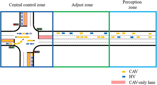
Before detailed descriptions of the control architecture, the layout of an intersection is first introduced. The space of an intersection and its link can be divided into three parts: perception zone, adjust zone, and central control zone, as illustrated in Figure 1. The control system architecture operates as follows. The controllers of an intersection are composed of a central controller and a number of on-board controllers. The central controller has two control layers: an intersection optimization control layer and a platoon management layer. The purpose of this study is to provide an optimized practicable platoon configuration according to the requirement of the intersection optimization control layer. The intersection optimization control layer mainly focuses on the central control zone. It optimizes the signal timing, CAVs trajectories in the central control zone, and the expectation platoon configuration, including the number of platoons, size of each platoon, and turn of each platoon.

Figure 1. Intersection zone division illustration.

To clearly state the platoon management problem, the following simplifications and assumptions are made:

• The central controller can accurately receive the latest state of all CAVs without delays.

• Every manually driven vehicle immediately leaves dedicated CAV lanes once it enters the adjust zone.

• Vehicles can only move forward.

• The destination link of a vehicle does not change after the vehicle enters the perception zone.

• Each CAV can accurately execute the instructions provided by its on-board controller.

• Since dedicated CAV lanes are on the left side of each link, only left-turn CAVs and straight-going CAVs use the dedicated CAV lanes.

As shown in Figure 1, there are seven CAVs in the perception zone. The intersection optimization control layer is expected to improve the traffic performance by forming the seven CAVs in a straight platoon and a left-turn platoon. However, the expectation platoon configuration only with a final state is not sufficient, as there are different orders to form the final configuration. Note different orders have different impacts on the traffic flow. Under extreme cases, this platoon configuration could even be hardly realized given the influence of manually driven vehicles and the length of the adjust zone. As a result, the expectation platoon configuration needs to be delivered to the platoon management layer at first instead of directly sent to decentralized controllers on CAVs, i.e., on-board controllers. In doing so, the platoon management layer transfers the expectation platoon configuration given by the intersection optimization control layer to a practicable platoon configuration while considering the initial states of CAVs. This practicable platoon configuration should be feasible for CAVs, and also as similar as possible to the expectation platoon configuration. The expectation platoon configuration considers the number of platoons, size of each platoon, and turn of each platoon. In the practicable platoon configuration, not only the number of platoons, size of each platoon, and turn of each platoon are considered, the order and lane number of each CAV are also determined. Then the practicable platoon configuration is sent to on-board controllers of CAVs. The on-board controllers of CAVs would adjust driving strategies to meet the practicable platoon configuration.

As described above, the inputs of the platoon management layer are the expectation platoon configuration and initial states of CAVs, and the output is a practicable platoon configuration. Therefore, the platoon management layer aims to realize two objectives. First, the layer should provide a practical platoon configuration as output. For instance, the overtaking and number of lane change should be optimized, which leads to less traffic perturbations. Second, the difference between the expected and practical configurations is to be minimized.

2.2. Notations

The main notations applied hereafter are summarized in Table 1, which will be explained in detail in the formulations section.

Table 1. Notations.

General notations
$\mathrm{M}:$	A sufficiently large number
I:	Set of all CAVs
$\mathrm{N}:$	Number of all CAVs
${\mathrm{N}}_{\text{COL}}:$	Number of CAVs using dedicated CAV lanes to pass the intersection
$\mathrm{T}:$	Control time horizon
${\mathrm{N}}_{\mathrm{P}}:$	Number of platoons given by central controller
${\mathit{J}}_{\mathit{c}}:$	Set of all dedicated CAV lanes
${\mathit{J}}_{{\mathit{i}}^{\mathit{\text{turn}}}}:$	Set of lanes which lanes allocation is same with the turn of vehicle i
Parameters
k 1:	Weight of difference of platoon size
k2:	Weight of number of lane change
k3:	Weight of distance to the end of adjust zone at time T
$\Delta t:$	Unit time
tk:	Planned arrival time of the first CAV in platoon k by the central controller
${\gamma }_i^{\mathit{\text{turn}}}:$	0, if vehicle i go straight; 1, if vehicle i turn left
${\gamma }_o^{\mathit{\text{turn}}}:$	0, if the first platoon goes straight; 1, if the first platoon turn left
Lk:	Number of vehicles in platoon k given by central controller
xend:	The position of the end of the adjust zone
vmin:	The minimum speed of vehicles, m/s
vmax:	The maximum speed of vehicles, m/s
amin:	The minimum acceleration of vehicles, $m/s^2$
amax:	The maximum acceleration of vehicles, $m/s^2$
Decision variables
σi:	Output order of CAV i, integer between 0 and NCOL
$x_i(t):$	Longitudinal position of vehicle i at time t
${\zeta }_i^j(t):$	1, if vehicle i is in lanes j at time t; 0, otherwise
Auxiliary variables
$\Delta L_j:$	Difference of length of planned platoon j with asked platoon length
$O_i(t):$	1, if vehicle i changing lanes at time t; 0, otherwise
${\epsilon }_i^l:$	1, if vehicle i is the last vehicle of a platoon; 0, otherwise
${\epsilon }_i^f:$	1, if vehicle i is the first vehicle of a platoon; 0, otherwise
Ei:	Index of the platoon which vehicle i belongs to
${\theta }_{i{i}^{\prime }}:$	0, if σi larger than ${\sigma }_{i^{\prime }};$ 1, otherwise
${\eta }_{i{i}^{\prime }}(t):$	0, if vehicle i is behind vehicle $i^{\prime }$ at time t; 1, otherwise
${\xi }_{\mathit{\text{ij}}}^E:$	0, if Ei larger than j; 1, otherwise
${\theta }_{i{i}^{\prime }}^{\mathit{\text{turn}}}:$	1, if both vehicle i and vehicle $i^{\prime }$ are going straight; 0, otherwise
$L_{i{i}^{\prime }}^a:$	0, if the output length of platoon that vehicle i belongs to is shorter than expected length; 1, otherwise
$v_i(t):$	the speed of vehicle i at time t
${\rho }_{i{i}^{\prime }(t)}:$	correlation or interaction between the vehicle i and vehicle $i^{\prime }$
$a_i(t):$	the acceleration of vehicle i at time t

3. Formulations

This section presents the developed MILP formulation. The objective function is initially constructed, followed by detailed descriptions of various constraints and a summary of the formulation.

3.1. Objective function

The objective function is composed of three items: minimizing the difference between the output practicable platoon configuration and the input expectation one, minimizing the influence of platoon formation, and minimizing the travel time of vehicles in the adjust zone.

In the first item, the difference between the output practicable platoon configuration and the input expectation platoon configuration given by the intersection control algorithm is defined as the sum of the absolute value of the difference of platoon size. The platoon length difference of platoon k is indicated by $\Delta L_k$ as shown in Eq. (1)(1) $$\mathrm{\text{min}}{k}_1\sum _{j=0}^{N_P}\Delta L_k+k_2\sum _{i=0}^N\sum _{t=0}^T{O}_i(t)+k_3\sum _{i=0}^N\left(x_{\mathit{\text{end}}}-x_i(T)\right)$$(1) .

In the second item, lane changes are considered to represent the influence of platoon formation, since they change vehicles’ orders. Thus, the number of lane change is used to evaluate the influence of platoon formation. The number of lane change of all CAVs in the control time horizon is indicated by ${\sum }_{i=0}^{N-1}{\sum }_{t=0}^{T-1}{O}_i(t)$ as shown in Eq. (1)(1) $$\mathrm{\text{min}}{k}_1\sum _{j=0}^{N_P}\Delta L_k+k_2\sum _{i=0}^N\sum _{t=0}^T{O}_i(t)+k_3\sum _{i=0}^N\left(x_{\mathit{\text{end}}}-x_i(T)\right)$$(1) .

In the third item, minimizing the travel time of vehicles in the adjust zone is transferred to minimize the gap between the final longitudinal position and the stop line. It is indicated by $x_{\mathit{\text{end}}}-x_i(T)$ as shown in Eq. (1)(1) $$\mathrm{\text{min}}{k}_1\sum _{j=0}^{N_P}\Delta L_k+k_2\sum _{i=0}^N\sum _{t=0}^T{O}_i(t)+k_3\sum _{i=0}^N\left(x_{\mathit{\text{end}}}-x_i(T)\right)$$(1) .

Therefore, the objective function of the proposed MILP model is constructed as (1) $$\mathrm{\text{min}}{k}_1\sum _{j=0}^{N_P}\Delta L_k+k_2\sum _{i=0}^N\sum _{t=0}^T{O}_i(t)+k_3\sum _{i=0}^N\left(x_{\mathit{\text{end}}}-x_i(T)\right)$$(1)

3.2. Constraints

This section introduces six constraint groups: vehicle motion constraints, vehicle order constraints, platoon splitting constraints, platoon number constraints, platoon rationality constraints, and objective auxiliary variable constraints.

3.2.1. Vehicle motion constraints

Vehicle motion constraints are composed of longitudinal motion constraints, lateral motion constraints, and safety constraints.

1. Longitudinal motion constraints. The longitudinal motion speed and acceleration should be limited to a reasonable range as Eq. (2)(2) $$v_i(t)=\frac{x_i(t)-x_i(t-1)}{\Delta t},\forall i\in I,t\in [1,T]$$(2) to Eq. (5)(5) $$a_{\mathrm{\text{max}}}\ge a_i(t)\ge a_{\mathrm{\text{min}}},\forall i\in I,t\in [1,T]$$(5) : (2) $$v_i(t)=\frac{x_i(t)-x_i(t-1)}{\Delta t},\forall i\in I,t\in [1,T]$$(2) (3) $$a_i(t)=\frac{v_i(t)-v_i(t-1)}{\Delta t},\forall i\in I,t\in [1,T]$$(3) (4) $$v_{\mathrm{\text{max}}}\ge v_i(t)\ge v_{\mathrm{\text{min}}},\forall i\in I,t\in [1,T]$$(4) (5) $$a_{\mathrm{\text{max}}}\ge a_i(t)\ge a_{\mathrm{\text{min}}},\forall i\in I,t\in [1,T]$$(5)

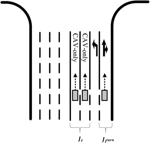
2. Lateral motion constraints. First, there is at most one lane change maneuver per time step, and vehicles can only change lanes one time per time step. Second, each vehicle has to occupy one and only one lane per time step. Third, CAVs have to move to the assigned lanes at the final state, as shown in Figure 2. These three lateral motion constraints are formulated as Eq. (6)(6) $${\zeta }_i^j(t)\le {\zeta }_i^j(t-1)+{\zeta }_i^{j-1}(t-1)+{\zeta }_i^{j+1}(t-1),\forall i\in I,t\in [1,T],j\in L$$(6) to Eq. (8)(8) $$\sum _{j\in J_c\cup J_{i^{\mathit{\text{turn}}}}}{\zeta }_i^j(T-1)=1,\forall i\in I,t\in [0,T]$$(8) , respectively. (6) $${\zeta }_i^j(t)\le {\zeta }_i^j(t-1)+{\zeta }_i^{j-1}(t-1)+{\zeta }_i^{j+1}(t-1),\forall i\in I,t\in [1,T],j\in L$$(6) (7) $$\sum _{j\in J}{\zeta }_i^j(t)=1,\forall i\in I,t\in [0,T]$$(7) (8) $$\sum _{j\in J_c\cup J_{i^{\mathit{\text{turn}}}}}{\zeta }_i^j(T-1)=1,\forall i\in I,t\in [0,T]$$(8)

3. Safety constraints. Eqs. (9)(9) $$\begin{array}{l}{x}_{i^{\prime }}(t)-(3-{\eta }_{i{i}^{\prime }}(t)-{\zeta }_{i^{\prime }}^j(t)-{\zeta }_i^j(t))M+L_{\mathit{\text{car}}}+\\ \Delta t\mathrm{\text{min}}[\frac{v_{\mathrm{\text{max}}}}{2},\frac{v_{i^{\prime }}(t)-v_i(t)+(a_{\mathrm{\text{max}}}-a_{\mathrm{\text{min}}})\Delta t}{2}]\le x_i(t),\forall i,i^{\prime }\in I,t\in [0,T],j\in L\end{array}$$(9) and (10)(10) $$\begin{array}{l}{x}_{i^{\prime }}(t)+(2+{\eta }_{i{i}^{\prime }}(t)-{\zeta }_{i^{\prime }}^j(t)-{\zeta }_i^j(t))M\ge x_i(t)+L_{\mathit{\text{car}}}+\\ \Delta t\mathrm{\text{min}}[\frac{v_{\mathrm{\text{max}}}}{2},\frac{v_i(t)-v_{i^{\prime }}(t)+(a_{\mathrm{\text{max}}}-a_{\mathrm{\text{min}}})\Delta t}{2}],\forall i,i^{\prime }\in I,t\in [0,T],j\in L\end{array}$$(10) are established to ensure that the longitudinal distance between any two vehicles in the same lanes is larger than a safety gap. The safety gap is set to keep safety, and its value is flexibly designed. It should not be too large, and it also needs to avoid the situation where a following vehicle jumps to the front of its leading vehicle per time step. (9) $$\begin{array}{l}{x}_{i^{\prime }}(t)-(3-{\eta }_{i{i}^{\prime }}(t)-{\zeta }_{i^{\prime }}^j(t)-{\zeta }_i^j(t))M+L_{\mathit{\text{car}}}+\\ \Delta t\mathrm{\text{min}}[\frac{v_{\mathrm{\text{max}}}}{2},\frac{v_{i^{\prime }}(t)-v_i(t)+(a_{\mathrm{\text{max}}}-a_{\mathrm{\text{min}}})\Delta t}{2}]\le x_i(t),\forall i,i^{\prime }\in I,t\in [0,T],j\in L\end{array}$$(9) (10) $$\begin{array}{l}{x}_{i^{\prime }}(t)+(2+{\eta }_{i{i}^{\prime }}(t)-{\zeta }_{i^{\prime }}^j(t)-{\zeta }_i^j(t))M\ge x_i(t)+L_{\mathit{\text{car}}}+\\ \Delta t\mathrm{\text{min}}[\frac{v_{\mathrm{\text{max}}}}{2},\frac{v_i(t)-v_{i^{\prime }}(t)+(a_{\mathrm{\text{max}}}-a_{\mathrm{\text{min}}})\Delta t}{2}],\forall i,i^{\prime }\in I,t\in [0,T],j\in L\end{array}$$(10)

Figure 2. Illustration of available lanes for a CAV going straight.

where ${\eta }_{i{i}^{\prime }}^j(t)$ shows the longitudinal position relationship and L_car shows the vehicle length. If vehicle i is in front of vehicle $i^{\prime }$ in the same lane, ${\eta }_{i{i}^{\prime }}^j(t)=1.$ The expression min $[\frac{v_{\mathrm{\text{max}}}}{2},$ $\frac{v_i(t)-v_{i^{\prime }}(t)+a_{\mathrm{\text{max}}}-a_{\mathrm{\text{min}}}}{2}]$ means taking the smaller of two terms, where v_max represents the maximum speed of the vehicle, $v_i(t)$ represents the speed of the vehicle i at time t, $v_{i^{\prime }}(t)$ represents the speed of the vehicle i’ at time t, $a_{\mathrm{\text{max}}}/a_{\mathrm{\text{min}}}$ represents the maximum/minimum acceleration of the vehicle, and $\Delta t$ is the unit time. The second term of the expression is the average speed of the front car braking sharply and the rear car accelerating uniformly at the maximum acceleration. In both cases, it is necessary to maintain a safe headway, which can avoid collisions or dangerous situations between vehicles.

Since the longitudinal position should be as large as possible (in order to minimize the gap between the final longitudinal position and the stop line) according to the objective function, vehicles prefer to select small space headway. As a result, Eqs. (9)(9) $$\begin{array}{l}{x}_{i^{\prime }}(t)-(3-{\eta }_{i{i}^{\prime }}(t)-{\zeta }_{i^{\prime }}^j(t)-{\zeta }_i^j(t))M+L_{\mathit{\text{car}}}+\\ \Delta t\mathrm{\text{min}}[\frac{v_{\mathrm{\text{max}}}}{2},\frac{v_{i^{\prime }}(t)-v_i(t)+(a_{\mathrm{\text{max}}}-a_{\mathrm{\text{min}}})\Delta t}{2}]\le x_i(t),\forall i,i^{\prime }\in I,t\in [0,T],j\in L\end{array}$$(9) and (10)(10) $$\begin{array}{l}{x}_{i^{\prime }}(t)+(2+{\eta }_{i{i}^{\prime }}(t)-{\zeta }_{i^{\prime }}^j(t)-{\zeta }_i^j(t))M\ge x_i(t)+L_{\mathit{\text{car}}}+\\ \Delta t\mathrm{\text{min}}[\frac{v_{\mathrm{\text{max}}}}{2},\frac{v_i(t)-v_{i^{\prime }}(t)+(a_{\mathrm{\text{max}}}-a_{\mathrm{\text{min}}})\Delta t}{2}],\forall i,i^{\prime }\in I,t\in [0,T],j\in L\end{array}$$(10) can be linearized as Eq. (11)(11) $$\begin{array}{l}{x}_{i^{\prime }}(t)-(3-{\eta }_{i{i}^{\prime }}(t)-{\zeta }_{i^{\prime }}^j(t)-{\zeta }_i^j(t)+{\rho }_{i{i}^{\prime }(t)})M+\Delta t\frac{v_{\mathrm{\text{max}}}}{2}\le x_i(t),\\ \forall i,i^{\prime }\in I,t\in [0,T],j\in L\end{array}$$(11) to Eq. (14)(14) $$\begin{array}{l}{x}_{i^{\prime }}(t)+(3+{\eta }_{i{i}^{\prime }}(t)-{\zeta }_{i^{\prime }}^j(t)-{\zeta }_i^j(t)-{\rho }_{i{i}^{\prime }(t)})M\ge x_i(t)+L_{\mathit{\text{car}}}+\\ \Delta t\frac{v_i(t)-v_{i^{\prime }}(t)+(a_{\mathrm{\text{max}}}-a_{\mathrm{\text{min}}})\Delta t}{2},\forall i,i^{\prime }\in I,t\in [0,T],j\in L\end{array}$$(14) . (11) $$\begin{array}{l}{x}_{i^{\prime }}(t)-(3-{\eta }_{i{i}^{\prime }}(t)-{\zeta }_{i^{\prime }}^j(t)-{\zeta }_i^j(t)+{\rho }_{i{i}^{\prime }(t)})M+\Delta t\frac{v_{\mathrm{\text{max}}}}{2}\le x_i(t),\\ \forall i,i^{\prime }\in I,t\in [0,T],j\in L\end{array}$$(11) (12) $$\begin{array}{c}{x}_{i^{\prime }}(t)+(2+{\eta }_{i{i}^{\prime }}(t)-{\zeta }_{i^{\prime }}^j(t)-{\zeta }_i^j(t)+{\rho }_{i{i}^{\prime }(t)})M\ge x_i(t)+\Delta t\frac{v_{\mathrm{\text{max}}}}{2},\\ \forall i,i^{\prime }\in I,t\in [0,T],j\in L\end{array}$$(12) (13) $$\begin{array}{l}{x}_{i^{\prime }}(t)-(4-{\eta }_{i{i}^{\prime }}(t)-{\zeta }_{i^{\prime }}^j(t)-{\zeta }_i^j(t)-{\rho }_{i{i}^{\prime }(t)})M+L_{\mathit{\text{car}}}+\\ \Delta t\frac{v_i(t)-v_{i^{\prime }}(t)+(a_{\mathrm{\text{max}}}-a_{\mathrm{\text{min}}})\Delta t}{2}\le x_i(t),\forall i,i^{\prime }\in I,t\in [0,T],j\in L\end{array}$$(13) (14) $$\begin{array}{l}{x}_{i^{\prime }}(t)+(3+{\eta }_{i{i}^{\prime }}(t)-{\zeta }_{i^{\prime }}^j(t)-{\zeta }_i^j(t)-{\rho }_{i{i}^{\prime }(t)})M\ge x_i(t)+L_{\mathit{\text{car}}}+\\ \Delta t\frac{v_i(t)-v_{i^{\prime }}(t)+(a_{\mathrm{\text{max}}}-a_{\mathrm{\text{min}}})\Delta t}{2},\forall i,i^{\prime }\in I,t\in [0,T],j\in L\end{array}$$(14) where ${\rho }_{i{i}^{\prime }(t)}$ is also an auxiliary variable for linearization, used to replace the original nonlinear constraint conditions and convert them into linear form. It ensures the space headway between two vehicles larger than $\frac{v_{\mathrm{\text{max}}}}{2}$ and $\frac{v_i(t)-v_{i^{\prime }}(t)+(a_{\mathrm{\text{max}}}-a_{\mathrm{\text{min}}})\Delta t}{2}.$ $v_{\mathrm{\text{max}}}/2$ represents half of the vehicle’s maximum velocity. When considered as uniformly decelerated linear motion, it is regarded as the average velocity during the deceleration process. To some extent, it represents the displacement during deceleration. This provides an ample buffer zone for vehicle travel, ensuring adaptability to various traffic conditions and speed changes, thereby preventing collisions or hazardous situations between vehicles.

3.2.2. Vehicle order constraints

Vehicle order is the order of a CAV in all CAVs. A CAV can use either dedicated CAV lanes or normal lanes to pass the intersection. If a CAV uses a dedicated CAV lane, it needs to join a platoon, and then the vehicle order makes sense. For CAVs not using dedicated CAV lanes, the vehicle order is useless, and it will be set to a meaningless value. This includes: reasonable order range constraints, unique order constraints, order–position relationship constraints, and non-dedicated CAV lane group order constraints. The first three groups of constraints are set for CAVs using dedicated CAV lanes to pass the intersection. The last group of constraints is set for CAVs not using dedicated CAV lanes to pass the intersection.

1. Reasonable order range constraints. For CAVs using dedicated CAV lanes to pass the intersection, their order should be in the range [0, N_COL), where N_COL is the number of CAVs using dedicated CAV lanes to pass the intersection. N_COL is indicated by ${\sum }_{i=0}^{N-1}\sum _{j_c\in J_c}{\zeta }_i^{j_c}(T),$ as shown in Eq. (15)(15) $$\sum _{i=0}^{N-1}\sum _{j_c\in J_c}{\zeta }_i^{j_c}(T)-1+(1-\sum _{j_c\in J_c}{\zeta }_i^{j_c}(T))M\ge {\sigma }_i\ge 0,\forall i\in I$$(15) . (15) $$\sum _{i=0}^{N-1}\sum _{j_c\in J_c}{\zeta }_i^{j_c}(T)-1+(1-\sum _{j_c\in J_c}{\zeta }_i^{j_c}(T))M\ge {\sigma }_i\ge 0,\forall i\in I$$(15)

2. Unique order constraints. For CAVs using dedicated CAV lanes to pass the intersection, each of them should have a unique order, which means their order is not equal to orders of other CAVs, as shown in Eqs. (16)(16) $${\sigma }_i-{\sigma }_{i^{\prime }}>-(2-\sum _{j_c\in J_c}{\zeta }_i^{j_c}(T)-\sum _{j_c\in J_c}{\zeta }_{i^{\prime }}^{j_c}(T)+{\theta }_{i{i}^{\prime }})M,\forall i,i^{\prime }\in I,i\ne i^{\prime }$$(16) and (17)(17) $${\sigma }_{i^{\prime }}-{\sigma }_i>-(3-\sum _{j_c\in J_c}{\zeta }_i^{j_c}(T)-\sum _{j_c\in J_c}{\zeta }_{i^{\prime }}^{j_c}(T)-{\theta }_{i{i}^{\prime }}),\forall i,i^{\prime }\in I,i\ne i^{\prime }$$(17) . (16) $${\sigma }_i-{\sigma }_{i^{\prime }}>-(2-\sum _{j_c\in J_c}{\zeta }_i^{j_c}(T)-\sum _{j_c\in J_c}{\zeta }_{i^{\prime }}^{j_c}(T)+{\theta }_{i{i}^{\prime }})M,\forall i,i^{\prime }\in I,i\ne i^{\prime }$$(16) (17) $${\sigma }_{i^{\prime }}-{\sigma }_i>-(3-\sum _{j_c\in J_c}{\zeta }_i^{j_c}(T)-\sum _{j_c\in J_c}{\zeta }_{i^{\prime }}^{j_c}(T)-{\theta }_{i{i}^{\prime }}),\forall i,i^{\prime }\in I,i\ne i^{\prime }$$(17)

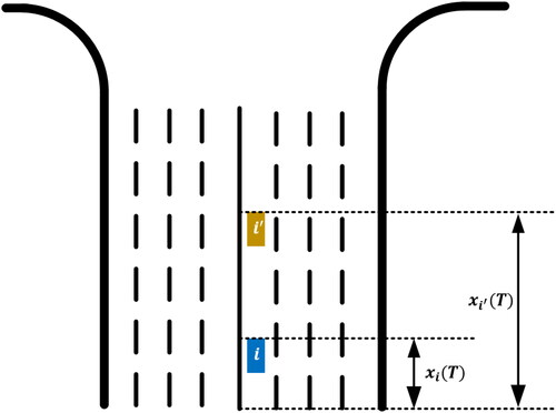
3. Order–position relationship constraints. The orders of CAVs are also related to longitudinal positions at the end of control time horizon. For instance, there are two CAVs, CAV i and CAV $i^{\prime },$ in Figure 3. Since $x_{i^{\prime }}(T)>x_i(T),$ CAV $i^{\prime }$ is in front of CAV i at the end of time horizon. CAV $i^{\prime }$ should have small order and leave the intersection earlier. It is guaranteed by Eqs. (18)(18) $${\sigma }_i-{\sigma }_{i^{\prime }}<3-{\eta }_{i{i}^{\prime }}(T)-{\zeta }_i^{j_c}(T)-{\zeta }_{i^{\prime }}^{j_c}(T),\forall i,i^{\prime }\in I,i\ne i^{\prime }$$(18) and (19)(19) $${\sigma }_{i^{\prime }}-{\sigma }_i>-(2+{\eta }_{i{i}^{\prime }}(T)-{\zeta }_i^{j_c}(T)-{\zeta }_{i^{\prime }}^{j_c}(T))M,\forall i,i^{\prime }\in I,i\ne i^{\prime }$$(19) . (18) $${\sigma }_i-{\sigma }_{i^{\prime }}<3-{\eta }_{i{i}^{\prime }}(T)-{\zeta }_i^{j_c}(T)-{\zeta }_{i^{\prime }}^{j_c}(T),\forall i,i^{\prime }\in I,i\ne i^{\prime }$$(18) (19) $${\sigma }_{i^{\prime }}-{\sigma }_i>-(2+{\eta }_{i{i}^{\prime }}(T)-{\zeta }_i^{j_c}(T)-{\zeta }_{i^{\prime }}^{j_c}(T))M,\forall i,i^{\prime }\in I,i\ne i^{\prime }$$(19)

4. Non-dedicated CAV lane group order constraints. For CAVs not using dedicated CAV lanes to pass the intersection, the order is meaningless. Their order is set as 2N, where N is the number of all CAVs. It is realized by Eq. (20)(20) $$2N\ge {\sigma }_i\ge \left(1-\sum _{j_c\in J_c}{\zeta }_i^{j_c}(T)\right)2N,\forall i\in I$$(20) . 2N is lager than N_NOL. (20) $$2N\ge {\sigma }_i\ge \left(1-\sum _{j_c\in J_c}{\zeta }_i^{j_c}(T)\right)2N,\forall i\in I$$(20)

Figure 3. Illustration of relationship between orders and final longitudinal position of CAVs.

3.2.3. Platoon splitting constraints

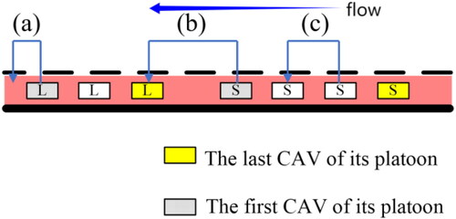
Platoon splitting is to split all CAVs using dedicated CAV lanes to pass the intersections in platoons. Platoon splitting can be realized by recognize critical CAVs. Critical CAVs include the first CAV and the last CAV in a platoon. As a result, there are three groups of constraints: last vehicle recognizing constraints, first vehicle recognizing constraints, and non-dedicated CAV lane group constraints.

1. Last vehicle recognizing constraints. ${\epsilon }_i^l$ is used to indicate whether vehicle i is the last vehicle of its platoon. Since the turns of each two adjacent platoons are different, the last vehicle can be judged by turns. There are four kinds of relationships between the turns of a vehicle and its following vehicle, as shown in Figure 4. For situation (a), the turns of a vehicle and its following vehicle are different. Thus, this vehicle is the last CAV of its platoon. It is guaranteed by Eq. (21)(21) $$\begin{array}{l}{\epsilon }_{i^{\prime }}^l\ge 1-\\ (2-\sum _{j_c\in J_c}{\zeta }_i^{j_c}(T)-\sum _{j_c\in J_c}{\zeta }_{i^{\prime }}^{j_c}(T)+{\sigma }_i-{\sigma }_{i^{\prime }}-1+2{\theta }_{i{i}^{\prime }}(N+1)+{\gamma }_i^{\mathit{\text{turn}}}+{\gamma }_{i^{\prime }}^{\mathit{\text{turn}}}-1+2{\theta }_{i{i}^{\prime }}^{\mathit{\text{turn}}})M,\forall i\in I,i^{\prime }\in I,i\ne i^{\prime }\end{array}$$(21) . In this study, vehicle turning is a binary variable. The turning of a vehicle is set as 0 if the vehicle goes straight, and its turning is set as 1 if it turns left. So ${\gamma }_i^{\mathit{\text{turn}}}+{\gamma }_{i^{\prime }}^{\mathit{\text{turn}}}=1$ means the front vehicle is the last vehicle of its platoon. (21) $$\begin{array}{l}{\epsilon }_{i^{\prime }}^l\ge 1-\\ (2-\sum _{j_c\in J_c}{\zeta }_i^{j_c}(T)-\sum _{j_c\in J_c}{\zeta }_{i^{\prime }}^{j_c}(T)+{\sigma }_i-{\sigma }_{i^{\prime }}-1+2{\theta }_{i{i}^{\prime }}(N+1)+{\gamma }_i^{\mathit{\text{turn}}}+{\gamma }_{i^{\prime }}^{\mathit{\text{turn}}}-1+2{\theta }_{i{i}^{\prime }}^{\mathit{\text{turn}}})M,\forall i\in I,i^{\prime }\in I,i\ne i^{\prime }\end{array}$$(21) For situation (b), there are no vehicles after the current vehicle, and it is also the last vehicle of its platoon, which is guaranteed by Eq. (22)(22) $${\epsilon }_{i^{\prime }}^l\ge 1+({\sigma }_i-\sum _{i=0}^{N-1}\sum _{j_c\in J_c}{\zeta }_i^{j_c}(T))-(1-\sum _{j_c\in J_c}{\zeta }_i^{j_c}(T))M,\forall i\in I$$(22) . The right part of Eq. (22)(22) $${\epsilon }_{i^{\prime }}^l\ge 1+({\sigma }_i-\sum _{i=0}^{N-1}\sum _{j_c\in J_c}{\zeta }_i^{j_c}(T))-(1-\sum _{j_c\in J_c}{\zeta }_i^{j_c}(T))M,\forall i\in I$$(22) equals 1 only when ${\sigma }_i={\sum }_{i=0}^{N-1}\sum _{j_c\in J_c}{\zeta }_i^{j_c}(T)$ and $\sum _{j_c\in J_c}{\zeta }_i^{j_c}(T)=1,$ which means the vehicle i is the last CAV in all CAVs using dedicated CAV lanes to pass the intersection. Otherwise, this constraint is released. (22) $${\epsilon }_{i^{\prime }}^l\ge 1+({\sigma }_i-\sum _{i=0}^{N-1}\sum _{j_c\in J_c}{\zeta }_i^{j_c}(T))-(1-\sum _{j_c\in J_c}{\zeta }_i^{j_c}(T))M,\forall i\in I$$(22) For situations (c) and (d), the current vehicle and its following vehicle both turn left or go straight. Thus, the current vehicle is not the last CAV of its platoon, which is guaranteed by Eqs. (23)(23) $$\begin{array}{l}{\epsilon }_{i^{\prime }}^l\le 2-\sum _{j_c\in J_c}{\zeta }_i^{j_c}(T)-\sum _{j_c\in J_c}{\zeta }_{i^{\prime }}^{j_c}(T)+{\sigma }_i-{\sigma }_{i^{\prime }}-1+2{\theta }_{i{i}^{\prime }}(N+1)+{\gamma }_i^{\mathit{\text{turn}}}+{\gamma }_{i^{\prime }}^{\mathit{\text{turn}}},\\ \forall i\in I,i^{\prime }\in I,i\ne i^{\prime }\end{array}$$(23) and (24)(24) $$\begin{array}{c}{\epsilon }_{i^{\prime }}^l\le 2-\sum _{j_c\in J_c}{\zeta }_i^{j_c}(T)-\sum _{j_c\in J_c}{\zeta }_{i^{\prime }}^{j_c}(T)+{\sigma }_i-{\sigma }_{i^{\prime }}-1+2{\theta }_{i{i}^{\prime }}(N+1)2-{\gamma }_i^{\mathit{\text{turn}}}-{\gamma }_{i^{\prime }}^{\mathit{\text{turn}}},\\ \forall i\in I,i^{\prime }\in I,i\ne i^{\prime }\end{array}$$(24) . (23) $$\begin{array}{l}{\epsilon }_{i^{\prime }}^l\le 2-\sum _{j_c\in J_c}{\zeta }_i^{j_c}(T)-\sum _{j_c\in J_c}{\zeta }_{i^{\prime }}^{j_c}(T)+{\sigma }_i-{\sigma }_{i^{\prime }}-1+2{\theta }_{i{i}^{\prime }}(N+1)+{\gamma }_i^{\mathit{\text{turn}}}+{\gamma }_{i^{\prime }}^{\mathit{\text{turn}}},\\ \forall i\in I,i^{\prime }\in I,i\ne i^{\prime }\end{array}$$(23) (24) $$\begin{array}{c}{\epsilon }_{i^{\prime }}^l\le 2-\sum _{j_c\in J_c}{\zeta }_i^{j_c}(T)-\sum _{j_c\in J_c}{\zeta }_{i^{\prime }}^{j_c}(T)+{\sigma }_i-{\sigma }_{i^{\prime }}-1+2{\theta }_{i{i}^{\prime }}(N+1)2-{\gamma }_i^{\mathit{\text{turn}}}-{\gamma }_{i^{\prime }}^{\mathit{\text{turn}}},\\ \forall i\in I,i^{\prime }\in I,i\ne i^{\prime }\end{array}$$(24) In the core constraint of situation (a), Eq. (22)(22) $${\epsilon }_{i^{\prime }}^l\ge 1+({\sigma }_i-\sum _{i=0}^{N-1}\sum _{j_c\in J_c}{\zeta }_i^{j_c}(T))-(1-\sum _{j_c\in J_c}{\zeta }_i^{j_c}(T))M,\forall i\in I$$(22) , an auxiliary variable ${\theta }_{i{i}^{\prime }}^{\mathit{\text{turn}}}$ is used to make sure that the turning judging term ${\gamma }_i^{\mathit{\text{turn}}}+{\gamma }_{i^{\prime }}^{\mathit{\text{turn}}}-1+2{\theta }_{i{i}^{\prime }}^{\mathit{\text{turn}}}$ is not smaller than 0. ${\theta }_{i{i}^{\prime }}^{\mathit{\text{turn}}}$ is limited as 1 if both vehicle i and vehicle $i^{\prime }$ go straight, i.e., ${\gamma }_i^{\mathit{\text{turn}}}={\gamma }_{i^{\prime }}^{\mathit{\text{turn}}}=0.$ Otherwise, ${\theta }_{i{i}^{\prime }}^{\mathit{\text{turn}}}$ is limited as 0. This is guaranteed by Eqs. (25)(25) $${\gamma }_i^{\mathit{\text{turn}}}+{\gamma }_{i^{\prime }}^{\mathit{\text{turn}}}<1+(1-{\theta }_{i{i}^{\prime }}^{\mathit{\text{turn}}})M,\forall i\in I,i^{\prime }\in I,i\ne i^{\prime }$$(25) and (26)(26) $${\gamma }_i^{\mathit{\text{turn}}}+{\gamma }_{i^{\prime }}^{\mathit{\text{turn}}}+{\theta }_{i{i}^{\prime }}^{\mathit{\text{turn}}}\ge 1,\forall i\in I,i^{\prime }\in I,i\ne i^{\prime }$$(26) . (25) $${\gamma }_i^{\mathit{\text{turn}}}+{\gamma }_{i^{\prime }}^{\mathit{\text{turn}}}<1+(1-{\theta }_{i{i}^{\prime }}^{\mathit{\text{turn}}})M,\forall i\in I,i^{\prime }\in I,i\ne i^{\prime }$$(25) (26) $${\gamma }_i^{\mathit{\text{turn}}}+{\gamma }_{i^{\prime }}^{\mathit{\text{turn}}}+{\theta }_{i{i}^{\prime }}^{\mathit{\text{turn}}}\ge 1,\forall i\in I,i^{\prime }\in I,i\ne i^{\prime }$$(26)

2. First vehicle recognizing constraints. ${\epsilon }_i^f$ is used to indicate whether vehicle i is the first vehicle of its platoon. Since the last vehicle of each platoon has been recognized, the first vehicle can be recognized according to the last vehicle. There are three kinds of relationships between a vehicle and its front vehicle, as shown in Figure 5. For situation (a), there is no front vehicle. The current vehicle is the first vehicle of its platoon, and it is guaranteed by Eq. (27)(27) $${\epsilon }_i^f\ge 1-{\sigma }_i,\forall i\in I$$(27) . The right term of Eq. (27)(27) $${\epsilon }_i^f\ge 1-{\sigma }_i,\forall i\in I$$(27) equals 1 only if ${\sigma }_i=0,$ which means the vehicle is the first CAV of all CAVs using dedicated CAV lanes to pass the intersection. Otherwise, this constraint is released. (27) $${\epsilon }_i^f\ge 1-{\sigma }_i,\forall i\in I$$(27) For situation (b), the front vehicle is the last vehicle of its platoon, so the current vehicle is the first vehicle of its platoon, which is guaranteed by Eq. (28)(28) $$\begin{array}{c}{\epsilon }_i^f\ge 1-(3-{\epsilon }_{i^{\prime }}^l-\sum _{j_c\in J_c}{\zeta }_i^{j_c}(T)-\sum _{j_c\in J_c}{\zeta }_{i^{\prime }}^{j_c}(T)+{\sigma }_i-{\sigma }_{i^{\prime }}-1+2{\theta }_{i{i}^{\prime }}(N+1)),\\ \forall i\in I,i^{\prime }\in I,i\ne i^{\prime }\end{array}$$(28) . (28) $$\begin{array}{c}{\epsilon }_i^f\ge 1-(3-{\epsilon }_{i^{\prime }}^l-\sum _{j_c\in J_c}{\zeta }_i^{j_c}(T)-\sum _{j_c\in J_c}{\zeta }_{i^{\prime }}^{j_c}(T)+{\sigma }_i-{\sigma }_{i^{\prime }}-1+2{\theta }_{i{i}^{\prime }}(N+1)),\\ \forall i\in I,i^{\prime }\in I,i\ne i^{\prime }\end{array}$$(28) For situation (c), the front vehicle is not the last vehicle of its platoon, so the current vehicle is not the first vehicle of its platoon, which is guaranteed by Eq. (29)(29) $$\begin{array}{c}{\epsilon }_i^f\le (2-\sum _{j_c\in J_c}{\zeta }_i^{j_c}(T)-\sum _{j_c\in J_c}{\zeta }_{i^{\prime }}^{j_c}(T)+{\epsilon }_{i^{\prime }}^l+{\sigma }_i-{\sigma }_{i^{\prime }}-1+2{\theta }_{i{i}^{\prime }}(N+1)),\\ \forall i\in I,i^{\prime }\in I,i\ne i^{\prime }\end{array}$$(29) . (29) $$\begin{array}{c}{\epsilon }_i^f\le (2-\sum _{j_c\in J_c}{\zeta }_i^{j_c}(T)-\sum _{j_c\in J_c}{\zeta }_{i^{\prime }}^{j_c}(T)+{\epsilon }_{i^{\prime }}^l+{\sigma }_i-{\sigma }_{i^{\prime }}-1+2{\theta }_{i{i}^{\prime }}(N+1)),\\ \forall i\in I,i^{\prime }\in I,i\ne i^{\prime }\end{array}$$(29)

3. Non-dedicated CAV lane group constraints. For CAVs not using dedicated CAV lanes to pass the intersection, they are neither the last CAV in their platoon nor the first CAV in their platoon. Thus, ${\epsilon }_i^l$ and ${\epsilon }_i^f$ are set as 0, which is guaranteed by Eqs. (30)(30) $${\epsilon }_i^f\le \sum _{j_c\in J_c}{\zeta }_i^{j_c}(T),\forall i\in I$$(30) and (31)(31) $${\epsilon }_i^l\le \sum _{j_c\in J_c}{\zeta }_i^{j_c}(T),\forall i\in I$$(31) : (30) $${\epsilon }_i^f\le \sum _{j_c\in J_c}{\zeta }_i^{j_c}(T),\forall i\in I$$(30) (31) $${\epsilon }_i^l\le \sum _{j_c\in J_c}{\zeta }_i^{j_c}(T),\forall i\in I$$(31)

Figure 4. Illustration of relationships between the turn of a vehicle and its following vehicle.

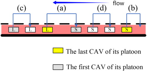
Figure 5. Illustration of relationships between a vehicle and its front vehicle.

3.2.4. Platoon number constraints

Vehicles forming platoons should have a reasonable platoon number. The platoon number of the first CAV is employed as a constraint at first. The platoon number of the following CAVs is restricted to the platoon splitting result. As a result, there are three groups of constraints: the first vehicle platoon number constraints, following vehicles platoon number constraints, and non-dedicated CAV lane group constraints.

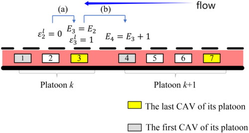
1. The first vehicle platoon number constraints. For the first CAV in all CAVs using dedicated CAV lanes to pass the intersection, its platoon is also the first platoon. So the platoon number of the first vehicle is set as 0 in Eq. (32)(32) $${\sigma }_{i}M\ge E_i\ge -{\sigma }_{i}M,\forall i\in I$$(32) : (32) $${\sigma }_{i}M\ge E_i\ge -{\sigma }_{i}M,\forall i\in I$$(32)

2. Following vehicles platoon number constraints. Platoon splitting is based on critical vehicles, and the last vehicles have been recognized. So the platoon number of each vehicle can be set according to the front vehicle. As shown in Figure 6, vehicle 2 is not the last vehicle of its platoon, so vehicle 3 and vehicle 2 belong to the same platoon and they should have the same platoon number. Since ${\epsilon }_2^l=0,$ E₃ can be set as $E_2+{\epsilon }_2^l.$ As for vehicle 3, which is the last vehicle of its platoon, vehicle 4 is in the next platoon of vehicle 3, so its platoon number should equal $E_3+1.$ Since ${\epsilon }_3^l=1,$ E₄ can also be expressed as $E_3+{\epsilon }_3^l.$ As a result, no matter under situation (a) or (b), the platoon number of the following vehicles can always be expressed as the sum of the platoon number and the binary variable indicating whether it is the last vehicle of the front vehicle by Eqs. (33)(33) $$\begin{array}{c}{E}_i\le {\epsilon }_{i^{\prime }}^l+E_{i^{\prime }}+(2-\sum _{j_c\in J_c}{\zeta }_i^{j_c}(T)-\sum _{j_c\in J_c}{\zeta }_{i^{\prime }}^{j_c}(T)+{\sigma }_i-{\sigma }_{i^{\prime }}-1+2{\theta }_{i{i}^{\prime }}(N+1))M,\\ \forall i\in I,i^{\prime }\in I,i\ne i^{\prime }\end{array}$$(33) and (34)(34) $$\begin{array}{c}{E}_i\ge {\epsilon }_{i^{\prime }}^l+E_{i^{\prime }}-(2-\sum _{j_c\in J_c}{\zeta }_i^{j_c}(T)-\sum _{j_c\in J_c}{\zeta }_{i^{\prime }}^{j_c}(T)+{\sigma }_i-{\sigma }_{i^{\prime }}-1+2{\theta }_{i{i}^{\prime }}(N+1))M,\\ \forall i\in I,i^{\prime }\in I,i\ne i^{\prime }\end{array}$$(34) . (33) $$\begin{array}{c}{E}_i\le {\epsilon }_{i^{\prime }}^l+E_{i^{\prime }}+(2-\sum _{j_c\in J_c}{\zeta }_i^{j_c}(T)-\sum _{j_c\in J_c}{\zeta }_{i^{\prime }}^{j_c}(T)+{\sigma }_i-{\sigma }_{i^{\prime }}-1+2{\theta }_{i{i}^{\prime }}(N+1))M,\\ \forall i\in I,i^{\prime }\in I,i\ne i^{\prime }\end{array}$$(33) (34) $$\begin{array}{c}{E}_i\ge {\epsilon }_{i^{\prime }}^l+E_{i^{\prime }}-(2-\sum _{j_c\in J_c}{\zeta }_i^{j_c}(T)-\sum _{j_c\in J_c}{\zeta }_{i^{\prime }}^{j_c}(T)+{\sigma }_i-{\sigma }_{i^{\prime }}-1+2{\theta }_{i{i}^{\prime }}(N+1))M,\\ \forall i\in I,i^{\prime }\in I,i\ne i^{\prime }\end{array}$$(34)

3. Non-dedicated CAV lane group constraints. For CAVs not using dedicated CAV lanes to pass the intersection, the platoon number is also meaningless. Similar to the vehicle order constraints, the platoon number is also set as a large enough number $2N_P,$ where N_P is the number of platoons given in the input platoon configuration. It is realized by Eq. (35)(35) $$2N_P\ge E_i\ge 2N_P(1-\sum _{j_c\in J_c}{\zeta }_i^{j_c}(T)),\forall i\in I$$(35) . (35) $$2N_P\ge E_i\ge 2N_P(1-\sum _{j_c\in J_c}{\zeta }_i^{j_c}(T)),\forall i\in I$$(35)

Figure 6. Illustration of following vehicles platoon number situations.

3.2.5. Platoon rationality constraints

The purpose of this section is to guarantee the rationality of the output platoon configuration. Three aspects are considered in this section: the platoon number should equal the required number, the turning of each platoon should equal the required turning, and the platoons can reach the stop line in time.

1. Platoon number constraints. Since each platoon only has one last vehicle, the number of platoons equals the number of all last vehicles. And the number should equal the required platoon number N_P as shown in Eq. (36)(36) $$\sum _{i=0}^{N-1}{\epsilon }_i^l=N_P$$(36) . (36) $$\sum _{i=0}^{N-1}{\epsilon }_i^l=N_P$$(36)

2. Platoon turning constraints. Since the turns of each pair of adjacent platoons are different, the turn of each platoon can be guaranteed as the same as the required turns, only if the turn of the first platoon is the same as the required turn: (37) $${\gamma }_o^{\mathit{\text{turn}}}+{\sigma }_i\ge {\gamma }_i^{\mathit{\text{turn}}}\ge {\gamma }_o^{\mathit{\text{turn}}}-{\sigma }_i,\forall i\in I$$(37) where ${\gamma }_o^{\mathit{\text{turn}}}$ is the required turn of the first platoon. Eq. (37)(37) $${\gamma }_o^{\mathit{\text{turn}}}+{\sigma }_i\ge {\gamma }_i^{\mathit{\text{turn}}}\ge {\gamma }_o^{\mathit{\text{turn}}}-{\sigma }_i,\forall i\in I$$(37) only works when ${\sigma }_i=0,$ or this constraint is released.

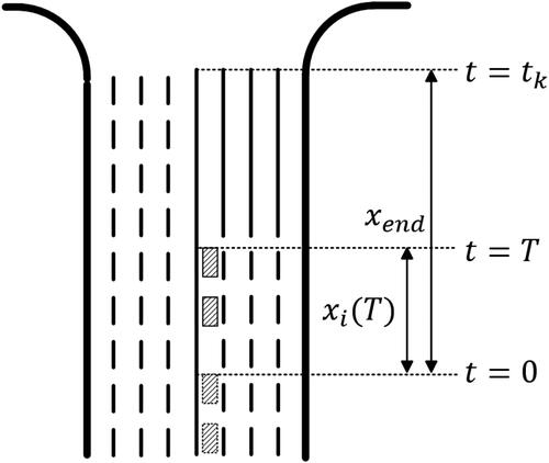
3. Platoon arriving time constraints. For a first vehicle i in its platoon, as shown in Figure 7, the final longitudinal position of it is $x_i(T).$ The distance to the stop line is $x_{\mathit{\text{end}}}-x_i(T),$ while the time it can utilize to driving to the stop line is $t_k-T,$ where t_k is the required arriving time of platoon k. Vehicle i needs to reach the stop line in time with a legal speed. It is guaranteed by Eq. (38)(38) $$x_{\mathit{\text{end}}}-x_i(T)\le \left(1-{\epsilon }_i^f+E_i-k+{\xi }_{\mathit{\text{ik}}}^E{N}_P\right)M+v_{\mathrm{\text{max}}}(t_j-T),\forall i\in I,j=0,1,\dots N_P-1$$(38) . (38) $$x_{\mathit{\text{end}}}-x_i(T)\le \left(1-{\epsilon }_i^f+E_i-k+{\xi }_{\mathit{\text{ik}}}^E{N}_P\right)M+v_{\mathrm{\text{max}}}(t_j-T),\forall i\in I,j=0,1,\dots N_P-1$$(38) where ${\xi }_{\mathit{\text{ik}}}^E$ is an auxiliary variable to ensure that the platoon number judging term $E_i-k+{\xi }_{\mathit{\text{ik}}}^E{N}_P$ is not smaller than 0. ${\xi }_{\mathit{\text{ik}}}^E=1$ if $E_i<k,$ otherwise ${\xi }_{\mathit{\text{ik}}}^E$ is set as 0. It is guaranteed by Eqs. (39)(39) $$E_i+{\xi }_{\mathit{\text{ik}}}^{E}M\ge k,\forall i\in I,\forall j=0,\dots ,N_P-1$$(39) and (40)(40) $$k+\left(1-{\xi }_{\mathit{\text{ik}}}^E\right)M>E_i,\forall i\in I,\forall j=0,\dots ,N_P-1$$(40) . (39) $$E_i+{\xi }_{\mathit{\text{ik}}}^{E}M\ge k,\forall i\in I,\forall j=0,\dots ,N_P-1$$(39) (40) $$k+\left(1-{\xi }_{\mathit{\text{ik}}}^E\right)M>E_i,\forall i\in I,\forall j=0,\dots ,N_P-1$$(40)

Figure 7. Illustration of platoon arriving.

3.2.6. Objective auxiliary variable constraints

There are two auxiliary variables in the objective function, platoon length gap $\Delta L_k$ and number of lane change $O_i(t).$

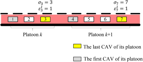
1. Platoon length gap constraints. In the final state, vehicle orders in the same platoon are continued. The output platoon length can be calculated according to vehicle order. For the first platoon, since the vehicle order of the first vehicle is 0, the length of the first platoon should equal the vehicle order of the last vehicle plus one, as shown in Eqs. (41)(41) $$\Delta L_k\ge {\sigma }_i+1-L_k-\left(1-{\epsilon }_i^l+E_i\right)M,\forall i\in I,i^{\prime }\in I,i\ne i^{\prime }$$(41) and (42)(42) $$\Delta L_k\ge L_k-{\sigma }_i-1-\left(1-{\epsilon }_i^l+E_i\right)M,\forall i\in I,i^{\prime }\in I,i\ne i^{\prime }$$(42) . (41) $$\Delta L_k\ge {\sigma }_i+1-L_k-\left(1-{\epsilon }_i^l+E_i\right)M,\forall i\in I,i^{\prime }\in I,i\ne i^{\prime }$$(41) (42) $$\Delta L_k\ge L_k-{\sigma }_i-1-\left(1-{\epsilon }_i^l+E_i\right)M,\forall i\in I,i^{\prime }\in I,i\ne i^{\prime }$$(42) For other platoons, the platoon length equals the vehicle order of its last vehicle minus the vehicle order of the last vehicle of the front platoon. For instance, in Figure 8, the last vehicle of platoon k is vehicle 3, while the last vehicle of platoon k + 1 is vehicle 7. The length of platoon k + 1 thus equals $7-3=4.$ This process can be expressed in Eqs. (43)(43) $$\begin{array}{c}\Delta L_k\ge L_k-\left({\sigma }_{i^{\prime }}-{\sigma }_i\right)-\\ \left(2-{\epsilon }_i^l-{\epsilon }_{i^{\prime }}^l+E_i-k+1+{\xi }_{\mathit{\text{ik}}-1}^E{N}_P+E_{i^{\prime }}-k+{\xi }_{i^{\prime }k}^E{N}_P+L_{i{i}^{\prime }}^a\right)M,\\ \forall i\in I,i^{\prime }\in I,i\ne i^{\prime }\end{array}$$(43) and (44)(44) $$\begin{array}{c}\Delta L_k\ge \left({\sigma }_{i^{\prime }}-{\sigma }_i\right)-L_k-\\ \left(2-{\epsilon }_i^l-{\epsilon }_{i^{\prime }}^l+E_i-k+1+{\xi }_{\mathit{\text{ik}}-1}^E{N}_P+E_{i^{\prime }}-k+{\xi }_{i^{\prime }k}^E{N}_P+1-L_{i{i}^{\prime }}^a\right)M,\\ \forall i\in I,i^{\prime }\in I,i\ne i^{\prime }\end{array}$$(44) . (43) $$\begin{array}{c}\Delta L_k\ge L_k-\left({\sigma }_{i^{\prime }}-{\sigma }_i\right)-\\ \left(2-{\epsilon }_i^l-{\epsilon }_{i^{\prime }}^l+E_i-k+1+{\xi }_{\mathit{\text{ik}}-1}^E{N}_P+E_{i^{\prime }}-k+{\xi }_{i^{\prime }k}^E{N}_P+L_{i{i}^{\prime }}^a\right)M,\\ \forall i\in I,i^{\prime }\in I,i\ne i^{\prime }\end{array}$$(43) (44) $$\begin{array}{c}\Delta L_k\ge \left({\sigma }_{i^{\prime }}-{\sigma }_i\right)-L_k-\\ \left(2-{\epsilon }_i^l-{\epsilon }_{i^{\prime }}^l+E_i-k+1+{\xi }_{\mathit{\text{ik}}-1}^E{N}_P+E_{i^{\prime }}-k+{\xi }_{i^{\prime }k}^E{N}_P+1-L_{i{i}^{\prime }}^a\right)M,\\ \forall i\in I,i^{\prime }\in I,i\ne i^{\prime }\end{array}$$(44)

2. Number of lane change constraints. The number of lane changes can be calculated with lane occupation ${\zeta }_i^j(t).$ Each vehicle can only occupy one lane at one time. If a vehicle occupies lane j at time t and then occupies an adjacent lane of lane j at time t + 1, a lane change is identified at time t. The number of lane change constraints is then expressed as follows as Eq. (45)(45) $$O_i(t)\ge {\zeta }_i^j(t)+{\zeta }_i^{j+1}(t+1)+{\zeta }_i^{j-1}(t+1)-1,\forall i\in I,t\in [0,T-1]$$(45) . (45) $$O_i(t)\ge {\zeta }_i^j(t)+{\zeta }_i^{j+1}(t+1)+{\zeta }_i^{j-1}(t+1)-1,\forall i\in I,t\in [0,T-1]$$(45)

Figure 8. Illustration of platoon length.

3.2.7. Optimization model summary

In summary, the decision variables vector of the proposed formulation is constructed as (46) $$\begin{array}{c}\mathit{x}=(x_1(1),\dots ,x_n(T),v_1(1),\dots ,v_n(T),a_1(1),\dots ,a_n(T),o_1(1),\dots ,o_n(T),{\zeta }_1^1(1),\dots ,\\ {\zeta }_n^J(T),{\sigma }_1,\dots ,{\sigma }_n,{\epsilon }_1^f,\dots ,{\epsilon }_n^f,{\epsilon }_1^l,\dots ,{\epsilon }_n^l,E_1,\dots ,E_n,{\theta }_{12},\dots ,{\theta }_{n(n-1)},{\theta }_{12}^{\mathit{\text{turn}}},\dots ,{\theta }_{n(n-1)}^{\mathit{\text{turn}}},\\ L_{12}^a,\dots ,L_{n(n-1)}^a,{\eta }_{12}(1),\dots ,{\eta }_{n(n-1)}(T),{\xi }_{11}^E,\dots ,{\xi }_{\mathit{\text{nP}}}^E,\Delta L_1,\dots ,\Delta L_P)\end{array}$$(46)

The dimension of decision variable is $(4+J)\mathit{\text{nT}}+(3+T)n(n-1)+(4+P)n+P,$ where n is number of vehicles, T is control time, J and P are the number of lanes and platoons, respectively. Besides, there are $4\mathit{\text{nT}}+1$ equality constraints and $4\mathit{\text{nTJ}}+n(T-1)J+15n(n-1)+12n+3\mathit{\text{np}}+n(T-1)+1$ inequality constraints. To establish a standard MILP formulation, each equality constraint can be further transferred to two inequality constraints. Thus, the model has entirely $4\mathit{\text{nTJ}}+n(T-1)J+15n(n-1)+12n+3\mathit{\text{np}}+8\mathit{\text{nT}}+n(T-1)+3$ standard constraints. Given all constraints and the objective function are linear, the proposed model is therefore a MILP formulation.

The dimension of the model is highly related to the number of vehicles. For instance, the optimization model has 403 decision variables and 1079 constraints with $T=10,J=3,P=4$ and the volume of 200 pcu/h. However, when the volume increases to 1200 pcu/h with other parameters unchanged, the model has 5386 decision variables and 9273 constraints. The computational efficiency is further discussed in Section 4.3.

4. Simulations

In this section, the simulation setup is first introduced. As summarized in Table 2, the simulations are designed and verified with respect to three aspects: (i) The correctness of microscopic vehicle motion driven by the proposed model. (ii) The broad adaptability of the proposed model through calculating the minimum length of adjust zone under different penetration and platoon rates. (iii) In order to guide the design of the traffic controller, two simulation parameters, i.e., platoon strength and platoon rate, are extensively analyzed. In the end, we discuss the computational efficiency of the proposed optimization model.

Table 2. Test scenarios.

Purpose	Scenario	Environment	Result
Microscope rationality	Vehicles form platoons	10 vehicles from platoons	Figure 12
Adaptability test	Test minimum adjust zone length under different volume	Penetration: 50%, platoon rate: 50%, left-turn ratio: 0.5	Figure 13
	Test minimum adjust zone length under different left-turn ratio	Volume: 1000 pcu/h, penetration: 50%, platoon rate: 80%
	Test minimum adjust zone length under different penetration	Volume: 1000 pcu/h, left-turn ratio: 0.5, platoon rate: 50%
	Test minimum adjust zone length under different platoon rate	Volume: 1000 pcu/h, left-turn ratio: 0.5, penetration: 50%
Control parameter test	Test number of lane changes under different platoon strength	Volume: 1000 pcu/h, left-turn ratio: 0.5	Figure 14
	Test number of lane changes under different platoon rate	Volume: 1000 pcu/h, left-turn ratio: 0.5

4.1. Simulations setup

The simulated arriving CAVs are generated randomly with Poisson distributions, as well as pre-defined left-turn ratio, penetration, and platoon rate. The left-turn ratio is the ratio of left-turning vehicles to all vehicles. The penetration rate refers to the ratio of CAVs to all vehicles, and the platoon rate is the ratio of CAVs forming platoons to all CAVs. The simulator decides whether a newly generated vehicle is a left-turn vehicle, whether a vehicle is a CAV, and whether a vehicle uses dedicated CAV lanes according to the simulation parameters randomly. As for the intersection space design, an intersection is divided into three parts, i.e., perception zone, adjust zone, and central control zone. The sum of the length of the intersection space is within certain communication range. Since the channelized part of arterial intersections in China is 100 m, the length of the simulated central control zone belonging to a link is also set as 100 m. According to several preliminary tests, the required length of the adjust zone never exceeds 100 m. Since vehicles in the perception zone need to be optimized in adjust zone, the length of the perception zone is set same with the length of the adjust zone. The objective function defined above consists of three terms: the size difference of the formation, the number of lanes, and the gap between the longitudinal position and the stop line. We adjust the importance of these three terms by introducing weight coefficients, namely, k1, k2, and k3. Given that the first term holds the highest significance and the third term primarily serves to eliminate exceptional solutions, such as vehicle standstill, we have employed the parameter settings, and during our simulations to make these adjustments. Regarding the lane configuration, both CAVs and conventional vehicles have dedicated right of way during the left-turn phase in the intersection, and there are no conflicts between left-turn and through movements. The lane configuration at the intersection is therefore realistic. Special CAV signal lights are required to indicate when CAV vehicles can proceed, stop, or execute specific maneuvers. Conventional lanes can use traditional traffic signal lights to control vehicle movement. According to relevant traffic regulations, it can be determined that the speed limits for automated driving tests in China may vary by region and specific test locations. Generally, in urban roads and residential areas, the testing speed is typically restricted to not exceed 30–50 km per hour based on Shanghai Municipal Management Measures for Intelligent Connected Vehicle Road Testing (Trial). The maximum speed constraint is set to maintain safe and stable vehicle operation in the simulation. Therefore, the maximum speed of each zone is set to 10 m/s.

Algorithm 1

Random platoon generation

1: Generate vehicles in perception zone according to Poisson distributions.

2: $N\Leftarrow$ vehicles number

3: while $N\ge 0$ do

4:  Generate random number r1, r2, and r3.

5:  if $r1\ge \text{left turn ratio}$ r_l then

6:   turn of the vehicle $\Leftarrow$ straight

7:  else

8:   turn of the vehicle $\Leftarrow$ left

9:  end if

10:  if $r2$< penetration p then

11:   the vehicle is CAV

12:  else

13:   the vehicle is not CAV

14:  end if

15:  if $r3$< platoon rate r_p and $r2$< penetration p then

16:   the vehicle use the dedicated CAV lane

17:  else

18:   the vehicle not use the dedicated CAV lane

19:  end if

20:  $N--$

21: end while

22: $N\Leftarrow$ vehicles number

23: while $N\ge 0$ do

24:  if the vehicle use the dedicated CAV lane then

25:   if record turn is null then

26:    record turn $\Leftarrow$ the turn of the vehicle

27:    platoon size $\Leftarrow 1$

28:   else

29:    if the turn of the vehicle $=$ record turn then

30:     platoon size $++$

31:    else

32:     generate a platoon

33:     record turn $\Leftarrow$ the turn of the vehicle

34:     platoon size $\Leftarrow 1$

35:    end if

36:   end if

37:  end if

38:  $N--$

39: end while

We first test the rationality and safety of the microscopic vehicle motions through visualizing vehicle trajectories. As for the second adaptability test, the vehicle platoon generation is shown in Algorithm 1. At first, vehicles are generated with Poisson distributions as well as simulated parameters. The simulator randomly determines whether the vehicle is a CAV and whether to use a CAV lane based on the simulation parameters. The trajectories of vehicles using the CAV lane are controlled by the model proposed in this article, while the other vehicles are assumed to pass through the intersection using the conventional lane with the correct lane function according to the existing rules of the intersection in China. If the generated CAV is assigned to use the dedicated CAV lane, it joins an existing platoon or starts a new platoon. Note all platoon configurations are provided as input from the traffic controller.

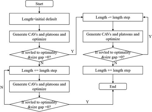
The length of both adjust zone and centralized control zone can not be dynamically changed considering the driving experience of drivers of regular vehicles on the road, while the length of the adjust zone should be limited in real applications. As a result, the minimum adjust zone is selected to test the adaptability. Since the adaptability test aims to find a similar minimum adjust zone length under different parameter settings, a specific test process is designed as shown in Figure 9. The length of the adjust zone is initialed as an certain value, e.g., 70 m. If the model is solved to be optimality and the sum of platoon size gap ${\sum }_{j=0}^{N_P}\Delta L_k$ is 0, the test process gradually reduces the adjust zone length and rerun the model, until the the sum of platoon size gap is larger than 0. Otherwise, a longer adjust zone is tested until ${\sum }_{j=0}^{N_P}\Delta L_k=0.$ The minimum adjust zone length is therefore can be obtained.

Figure 9. Adaptability test process.

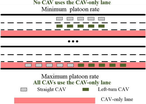
For the control parameter test, the vehicles are also generated according to Poisson distributions and pre-defined simulation parameters. Unlike the adaptability test, the expectation platoon configuration sent by the traffic controller is determined by two additional parameters, i.e., platoon strength and platoon rate. The platoon strength is defined as the ratio of average platoon length to the maximum platoon length, as illustrated in Figure 10. Similarly, the platoon ratio is the ratio of CAVs which use dedicated CAV lanes to pass an intersection, as shown in Figure 11. Consequently, the number of CAVs that need to form platoons is controlled by the platoon rate and CAVs number, and the average platoon length is determined by the number of CAVs those need to form platoons and the platoon strength. Finally, the control parameter test is repetitively simulated over different platoon strength and platoon rate settings.

Figure 10. Illustration of the platoon strength.

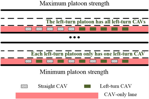
Figure 11. Illustration of the platoon rate.

4.2. Simulation results

This section reports the simulation results with respect to three purposes. Note that the optimization model has been solved to be optimality over all scenarios.

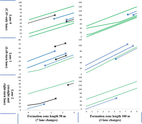
At first, the simulations for the rationality of microscopic vehicle motions with ten vehicles are conducted. Six out of ten vehicles are generated as CAVs and use dedicated CAV lanes to pass the intersection. The trajectories are illustrated in Figure 12, where each line represents a vehicle trajectory. The x-axis is the simulation time, while the y-axis is divided into three zones, which indicates different lanes. In each divided zone, the y-axis stands for longitudinal positions. The cross and circle are used to remark the lane changes: cross means the vehicle leaves the lane, while circle indicates the vehicle enters the lane. The solid lines represent trajectories of vehicles which are selected to use the dedicated CAV lane, while dash lines for other vehicles. The color of lines represents the number of lane changes: the green line means that the vehicle does not change its lane, while blue and black mean that the vehicle has one and two lane changes, respectively. As shown in Figure 12, two different adjust zone lengths are utilized for simulations. The adjust zone length indeed influences the number of lane changes, i.e., how the vehicles configure the platoon; when the adjust zone length is 100 m, only three vehicles need to change lanes, while with a 50 m adjust zone, five vehicles need to change lanes for seven times. It is also observed that vehicles form platoons and complete lane changes before the end of the adjust zone. Besides, vehicles complete the required platoon configuration without safety concerns. The simulated microscopic vehicle motions have been verified to be correct and rational.

Figure 12. Illustration of simulated vehicle trajectories. Cross and circle mark the start and the end of lane changes, respectively. Solid lines represent trajectories of vehicles using dedicated CAV lanes and different color means different numbers of lane changes.

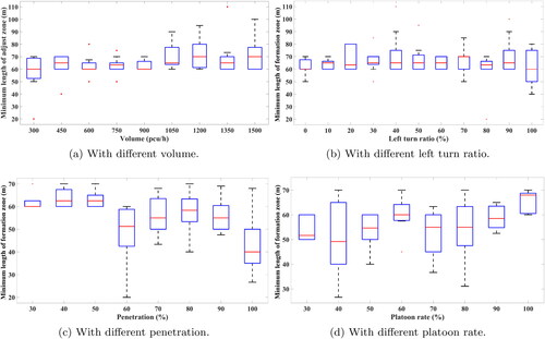
To demonstrate the broad adaptability of the proposed optimization model, we calculate the minimum adjust zone length over different parameters, including traffic volume, left-turn ratio, penetration, and platoon rates. The results are shown as Figure 13. It can be found that the average minimum length goes up slightly as the volume increases, and a higher volume typically leads to a larger minimum length of the adjust zone. On the contrary, the minimum adjust zone length is not sensitive to the left-turn ratio, penetration, and platoon rate. To ensure that the arriving vehicles successfully form a platoon configuration, the required minimum length of the adjust zone is similar. In practice, the length of the adjust zone can be adjusted dynamically according to the real-time traffic information. In conclusion, given a reasonable adjust zone length, the proposed optimization model can be effectively solved to be optimality over different scenarios.

Figure 13. The minimum length of adjust zone under different scenarios.

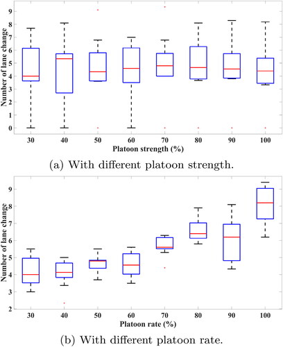
Finally, the impact of the platoon strength and platoon rate, which determine the expectation platoon configurations, is analyzed. The number of lane changes is adopted to evaluate the overall control performance, as lane changes can represent the disturbance to traffic flow when forming required platoon configurations. As shown in Figure 14, the number of lane changes remains stable when the platoon rate varies from 30% to 70%; then the number of lane changes has an ascending trend with further increasing the platoon rate. On the other hand, the number of lane changes to form the platoon is not sensitive to the platoon strength. Therefore, the traffic controller is recommended to adopt a platoon rate lower than 70% when the traffic demand is high, as well as a larger platoon strength to improve the overall traffic performance, such as a higher throughput and lower delay.

Figure 14. Simulation results of the control parameter test.

4.3. Computational efficiency

The computational efficiency is tested on a laptop with Intel i7-8550U CPU and 8G memory. According to the adaptability test results in Figure 13a, the lengths of the perception zone and the adjust zone are both set as 90 m. The maximum speed is set as 10 m/s, which is the same as the above tests. As a result, the minimum time to pass the perception zone is 9 s. The proposed optimization model is implemented in Python, and solved by Gurobi (Gurobi Optimization & Inc, 2019). Note that the model has been solved to be optimality in all scenarios.

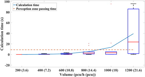
We first test the computational efficiency with different volumes. For each volume, the simulations are conducted for 100 times. The average calculation time is shown in Figure 15. It can be found that the model can be run less than 9 s when the volume is lower than 800 pcu/(h $·$ lane). It is argued that 800 pcu/(h $·$ lane) already corresponds to a large traffic demand since the traffic volume of peak hour is identified as less than 700 pcu/(h $·$ lane) (Singh & Saraswat, 2019).

Figure 15. Calculation efficiency with different volumes.

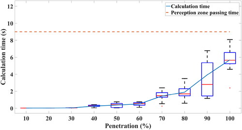
In addition, we test the influence of penetration rate with a fixed volume as 800 pcu/(h $·$ lane), and The simulations are repeated for 100 times under each penetration rate. As shown in Figure 16, the calculation time clearly increases with the penetration rate, while the calculation time never exceeds 9 s. Given that the minimum time to pass the intersection is 9 s, the optimization model thus can be iteratively run in real-time in practice.

Figure 16. Calculation efficiency with different penetrations.

5. Conclusion

This article has presented a platoon management algorithm at isolated intersections with dedicated CAV lanes or lane-allocation-free intersections under the mixed traffic environment. The intersection control structure is hierarchical where a central traffic controller is placed on top of the vehicle on-board vehicle controllers. We assume a central controller is in place to optimize signal timing and provide expectation platoon configurations. Then the proposed platoon management algorithm transfers the expectation platoon configurations to practicable platoon configurations, which will be executed by on-board controllers.

The objectives of the platoon formation model are minimizing the gap between the expectation platoon configuration and output practicable platoon configuration, minimizing influence to traffic flow, which is evaluated by the number of lane changes, and minimizing the travel time in the adjust zone. The proposed model is a MILP model and can run in real time.

A group of test scenarios are designed to test the rationality and adaptability of the proposed model. The micro-motion generated by the proposed model is proved to be rational. The model can adapt to different volumes, left-turn ratios, penetrations, and platoon rates. The model also explored the reasonable range of control parameters. The results show that the platoon rate needs to be lower than 70% when the volume is high in order to guarantee the platooning feasibility and reduce influence on other vehicles, while any platoon strength can be efficiently addressed. Thus, larger platoon strength is recommended for higher traffic throughput.

This article explores how to organize CAVs to form platoons with the expectation platoon configuration under the environment of mixed traffic. Further research could focus on a much detailed microscopic trajectory design and refine the differences in each lane change based on different target vehicles and traffic conditions. Additionally, replanning the trajectories of CAVs using normal lanes considering the interactions with manually driven vehicles is also an interesting topic.

Disclosure statement

No potential conflict of interest was reported by the author(s).

Additional information

Funding

This research was funded by the Shanghai Sailing Program [Grant No. 22YF1452600], the National Natural Science Foundation of China [Grant Nos. 51722809 and 61773293], the Short-term Visiting Abroad Scholarship of Tongji [Grant No. 201902006] and hosted by TU Delft. The views presented in this article are those of the authors alone.

References

- Bashiri, M., & Fleming, C. H. (2017). A platoon-based intersection management system for autonomous vehicles. In 2017 IEEE Intelligent Vehicles Symposium (IV), Los Angeles, CA, USA, June 11–14 (pp. 667–672). https://doi.org/10.1109/IVS.2017.7995794
- Baskar, L. D., De Schutter, B., Hellendoorn, J., & Papp, Z. (2011). Traffic control and intelligent vehicle highway systems: A survey. IET Intelligent Transport Systems, 5(1), 38–52. https://doi.org/10.1049/iet-its.2009.0001
- Cooper, C., Franklin, D., Ros, M., Safaei, F., & Abolhasan, M. (2016). A comparative survey of VANET clustering techniques. IEEE Communications Surveys & Tutorials, 19(1), 657–681. https://doi.org/10.1109/COMST.2016.2611524
- Dresner, K., Stone, P. (2004). Multiagent traffic management: A reservation-based intersection control mechanism. In Proceedings of the Third International Joint Conference on Autonomous Agents and Multiagent Systems – Volume 2, New York, NY, USA, July 19–23 (pp. 530–537).
- Du, Z., Chaudhuri, B. H., & Pisu, P. (2016). Distributed coordination of connected and automated vehicles at multiple interconnected intersections. World Academy of Science, Engineering and Technology, International Journal of Computer, Electrical, Automation, Control and Information Engineering, 10, 842–848.
- Faraj, M., Sancar, F. E., & Fidan, B. (2017). Platoon-based autonomous vehicle speed optimization near signalized intersections. In 2017 IEEE Intelligent Vehicles Symposium (IV), Los Angeles, CA, USA, June 11–14 (pp. 1299–1304). https://doi.org/10.1109/IVS.2017.7995891
- Guler, S. I., Menendez, M., & Meier, L. (2014). Using connected vehicle technology to improve the efficiency of intersections. Transportation Research Part C: Emerging Technologies, 46, 121–131. https://doi.org/10.1016/j.trc.2014.05.008
- Guo, Y., Ma, J., Xiong, C., Li, X., Zhou, F., & Hao, W. (2019). Joint optimization of vehicle trajectories and intersection controllers with connected automated vehicles: Combined dynamic programming and shooting heuristic approach. Transportation Research Part C: Emerging Technologies, 98, 54–72. https://doi.org/10.1016/j.trc.2018.11.010
- Gurobi Optimization, Inc. (2019). Gurobi optimizer reference manual. http://www.gurobi.com/
- Hall, R., & Chin, C. (2005). Vehicle sorting for platoon formation: Impacts on highway entry and throughput. Transportation Research Part C: Emerging Technologies, 13(5–6), 405–420. https://doi.org/10.1016/j.trc.2004.09.001
- He, Q., Head, K. L., & Ding, J. (2012). PAMSCOD: Platoon-based arterial multi-modal signal control with online data. Transportation Research Part C: Emerging Technologies, 20(1), 164–184. https://doi.org/10.1016/j.trc.2011.05.007
- Huang, X., & Peng, H. (2017). Speed trajectory planning at signalized intersections using sequential convex optimization. In 2017 American Control Conference (ACC), Seattle, WA, USA, May 24–26 (pp. 2992–2997). https://doi.org/10.23919/ACC.2017.7963406
- Jiang, Y., Li, S., & Shamo, D. E. (2006). A platoon-based traffic signal timing algorithm for major–minor intersection types. Transportation Research Part B: Methodological, 40(7), 543–562. https://doi.org/10.1016/j.trb.2005.07.003
- Lee, J., & Park, B. (2012). Development and evaluation of a cooperative vehicle intersection control algorithm under the connected vehicles environment. IEEE Transactions on Intelligent Transportation Systems, 13(1), 81–90. https://doi.org/10.1109/TITS.2011.2178836
- Li, Z., Elefteriadou, L., & Ranka, S. (2014). Signal control optimization for automated vehicles at isolated signalized intersections. Transportation Research Part C: Emerging Technologies, 49, 1–18. https://doi.org/10.1016/j.trc.2014.10.001
- Little, J. D., Kelson, M. D., & Gartner, N. H. (1981). Maxband: A versatile program for setting signals on arteries and triangular networks. Transportation Research Record, 795, 1–28.
- Liu, M., Wang, M., & Hoogendoorn, S. (2019). Optimal platoon trajectory planning approach at arterials. Transportation Research Record, 2673(9), 214–226. https://doi.org/10.1177/0361198119847474
- Li, L., & Wang, F.-Y. (2006). Cooperative driving at blind crossings using intervehicle communication. IEEE Transactions on Vehicular Technology, 55(6), 1712–1724. https://doi.org/10.1109/TVT.2006.878730
- Luo, F., Larson, J., & Munson, T. (2018). Coordinated platooning with multiple speeds. Transportation Research Part C: Emerging Technologies, 90, 213–225. https://doi.org/10.1016/j.trc.2018.02.011
- Memoli, S., Cantarella, G. E., de Luca, S., & Di Pace, R. (2017). Network signal setting design with stage sequence optimisation. Transportation Research Part B: Methodological, 100, 20–42. https://doi.org/10.1016/j.trb.2017.01.013
- Mohajerpoor, R., Saberi, M., & Ramezani, M. (2019). Analytical derivation of the optimal traffic signal timing: Minimizing delay variability and spillback probability for undersaturated intersections. Transportation Research Part B: Methodological, 119, 45–68. https://doi.org/10.1016/j.trb.2018.11.004
- Puthusseri, S. A. A. (2023). A self-enforced optimal framework for inter-platoon transfer in connected vehicles. Journal of Intelligent Transportation Systems, 27(4), 536–552. https://doi.org/10.1080/15472450.2022.2051169
- Qiu, J., Wu, G., Boriboonsomsin, K., & Barth, M. (2013). Platoon-based multi-agent intersection management for connected vehicle. In 2013 16th International IEEE Conference on Intelligent Transportation Systems – ITSC 2013, Hague, The Netherlands, October 6–9.
- Rakha, H., Ahn, K., & Kamalanathsharma, R. K. (2012). Eco-vehicle speed control at signalized intersections using I2V communication (Technical Report). US Department of Transportation.
- Rakha, H., Zohdy, I., Du, J., Park, B., Lee, J., & Elmetwally, M. (2011). Traffic signal control enhancements under vehicle infrastructure integration systems (Technical Report). US Department of Transportation.
- Rey, D., & Levin, M. W. (2019). Blue phase: Optimal network traffic control for legacy and autonomous vehicles. Transportation Research Part B: Methodological, 130, 105–129. https://doi.org/10.1016/j.trb.2019.11.001
- Schakel, W. J., Van Arem, B., & Netten, B. D. (2010). Effects of cooperative adaptive cruise control on traffic flow stability. In 13th International IEEE Conference on Intelligent Transportation Systems, Madeira, Portugal, September 19–22 (pp. 759–764).
- Singh, S. K., & Saraswat, A. (2019). Design service volume, capacity, level of service calculation and forecasting for a semi-urban city. Revue d’Intelligence Artificielle, 33(2), 139–143. https://doi.org/10.18280/ria.330209
- Tallapragada, P., & Cortés, J. (2019). Hierarchical-distributed optimized coordination of intersection traffic. IEEE Transactions on Intelligent Transportation Systems, 21(5), 2100–2113. https://doi.org/10.1109/TITS.2019.2912881
- Varaiya, P. (1993). Smart cars on smart roads: Problems of control. IEEE Transactions on Automatic Control, 38(2), 195–207. https://doi.org/10.1109/9.250509
- Wang, P., Jiang, Y., Xiao, L., Zhao, Y., & Li, Y. (2020). A joint control model for connected vehicle platoon and arterial signal coordination. Journal of Intelligent Transportation Systems, 24(1), 81–92. https://doi.org/10.1080/15472450.2019.1579093
- Wang, Z., Wu, G., Hao, P., & Barth, M. J. (2018). Cluster-wise cooperative eco-approach and departure application for connected and automated vehicles along signalized arterials. IEEE Transactions on Intelligent Vehicles, 3(4), 404–413. https://doi.org/10.1109/TIV.2018.2873912
- Webster, F. V. (1958). Traffic signal settings (Technical Report). Road Research Laboratory.
- Yu, C., Feng, Y., Liu, H. X., Ma, W., & Yang, X. (2018). Integrated optimization of traffic signals and vehicle trajectories at isolated urban intersections. Transportation Research Part B: Methodological, 112, 89–112. https://doi.org/10.1016/j.trb.2018.04.007
- Yu, C., Feng, Y., Liu, H. X., Ma, W., & Yang, X. (2019). Corridor level cooperative trajectory optimization with connected and automated vehicles. Transportation Research Part C: Emerging Technologies, 105, 405–421. https://doi.org/10.1016/j.trc.2019.06.002
- Zhang, Y., & Cao, G. (2011). V-PADA: Vehicle-platoon-aware data access in VANETs. IEEE Transactions on Vehicular Technology, 60(5), 2326–2339. https://doi.org/10.1109/TVT.2011.2148202
- Zhang, G., & Wang, Y. (2010). Optimizing minimum and maximum green time settings for traffic actuated control at isolated intersections. IEEE Transactions on Intelligent Transportation Systems, 12(1), 164–173. https://doi.org/10.1109/TITS.2010.2070795