HLPI-Ensemble: Prediction of human lncRNA-protein interactions based on ensemble strategy

ABSTRACT

LncRNA plays an important role in many biological and disease progression by binding to related proteins. However, the experimental methods for studying lncRNA-protein interactions are time-consuming and expensive. Although there are a few models designed to predict the interactions of ncRNA-protein, they all have some common drawbacks that limit their predictive performance. In this study, we present a model called HLPI-Ensemble designed specifically for human lncRNA-protein interactions. HLPI-Ensemble adopts the ensemble strategy based on three mainstream machine learning algorithms of Support Vector Machines (SVM), Random Forests (RF) and Extreme Gradient Boosting (XGB) to generate HLPI-SVM Ensemble, HLPI-RF Ensemble and HLPI-XGB Ensemble, respectively. The results of 10-fold cross-validation show that HLPI-SVM Ensemble, HLPI-RF Ensemble and HLPI-XGB Ensemble achieved AUCs of 0.95, 0.96 and 0.96, respectively, in the test dataset. Furthermore, we compared the performance of the HLPI-Ensemble models with the previous models through external validation dataset. The results show that the false positives (FPs) of HLPI-Ensemble models are much lower than that of the previous models, and other evaluation indicators of HLPI-Ensemble models are also higher than those of the previous models. It is further showed that HLPI-Ensemble models are superior in predicting human lncRNA-protein interaction compared with previous models. The HLPI-Ensemble is publicly available at: http://ccsipb.lnu.edu.cn/hlpiensemble/.

KEYWORDS:

• lncRNA
• lncRNA-protein interaction
• protein
• bioinformatics
• ensemble strategy

Introduction

Recent studies have shown that only a small number of human transcripts are involved in the protein translation process. Other RNAs which lack open reading frames and therefore can't translate into proteins are called noncoding RNA (ncRNA) [1]. Long non-coding RNA (lncRNA) is a type of ncRNA with a length between 200 nt and 100,000 nt, which is the main component of the transcripts. Many studies have shown that lncRNA plays an important role in many biological and pathological processes. For example, regulation of gene expression [2], transcription and post-translational regulation [3], chromatin modification [4,5], disease progression [6] and development [7–10]. In general, lncRNA performs its biological function by binding to the relevant protein [11,12]. Some experimental methods have been developed to identify lncRNA-protein interactions. For example, RNA immunoprecipitation and mass spectrometry are performed to identify lncRNA binding proteins [13]. However, the experimental study of lncRNA-protein interactions requires a great deal of resources. Fortunately, accumulated experimental data made it possible to predict lncRNA-protein interactions by computational methods.

During recent years, several computational methods have been proposed to predict lncRNA-protein interactions. In 2011, Bellucci et al. developed a computational model called CatRAPID [14]. The model introduced the biological properties of RNA and protein. For example, the secondary structure of RNA, the three-dimensional structure of protein, the hydrogen bond between RNA and protein, the van der Waals force and so on. In the same year, Muppirala et al. introduced a model called RPISeq [15], which contained two sub-models, respectively, trained by support vector machine (SVM) [16] and random forest (RF) [17]. RPISeq only applied sequence information to predict RNA-protein interactions. In 2013, Wang et al. proposed a classifier based on naive Bayesian and extended naive Bayesian [18]. The model introduced the properties of RNA and protein to produce triple features. Later, Lu et al. proposed a model called lncPro, which predicted the interactions of lncRNA-proteins by Fisher's linear discriminant analysis of amino acid and nucleotide sequences [19]. Recently, Suresh et al. developed a SVM classification model called RPI-Pred, which extracted RNA secondary structure features and protein three-dimensional structural features from RNA and protein sequences, respectively [20]. In 2016, Ge et al. developed a lncRNA-protein bipartite network inference (LPBNI) calculation method. LPBNI only used the known lncRNA-protein interactions to extrapolate the potential lncRNA-protein interactions [21]. In addition, Pan et al. developed a model called IPMiner by applying the stacked autoencoder to learn high-level features for predicting RNA-protein interactions from raw sequence composition features [22].

Although there are several models that can predict the lncRNA-protein interactions, they have some common drawbacks. First, the previous study attempted to construct a model to predict the RNA-protein interactions of all species. However, the homology of lncRNA is very weak, and there is a great difference between lncRNA in different species. Only 12% of human ncRNA can be found in other species. In addition, the training data for most previous models contained large amounts of mRNA. The mRNA refers to a class of RNA that can encode a protein, which is completely different from lncRNA. Application mRNA-protein data training model to predict lncRNA-protein interactions may reduce the accuracy of the model. Second, most of the previous models had a high false positive risk. The experimentally identified lncRNA-protein interactions account for only a small part. However, the predicting outcomes from most previous models showed that almost all of the unknown lncRNA-protein interactions were positive, indicating that the predicting outcomes are false positives (see “External validation” section). Third, the accuracy of previous prediction models was not high enough. Most of them applied only one type of lncRNA feature and one type of protein feature, which limited the comprehensiveness of the predictions.

In this study, we propose a new lncRNA-protein interactions prediction model called HLPI-Ensemble to solve the above problems. HLPI-Ensemble is specially designed for predicting human-related lncRNA-protein interactions, which is trained by human lncRNA-protein interactions data. We apply random pairing strategy to generate negative samples for lncRNA-protein interactions. The HLPI-Ensemble is based on the ensemble strategy. This strategy not only improves the prediction performance of model but also prevent the model from overfitting. Furthermore, HLPI-Ensemble employs three mainstream machine learning algorithm of SVM, RF and Extreme Gradient Boosting (XGB) [23] by ensemble strategy to generate HLPI-SVM Ensemble, HLPI-RF Ensemble, and HLPI-RF Ensemble, respectively. HLPI-SVM Ensemble, HLPI-RF Ensemble, and HLPI-XGB Ensemble achieve AUCs of 0.95, 0.96 and 0.96, respectively, in the test dataset. Moreover, in the external validation, we compare the performance of the HLPI-Ensemble models with the previous models by external validation. The test results show that the false positive (FP) of the HLPI-Ensemble models is much lower than that of the previous models. In addition, other evaluation indicators of the HLPI-Ensemble models are higher than those previous models. The HLPI-Ensemble is publicly available at: http://ccsipb.lnu.edu.cn/hlpiensemble/.

Results

Performance evaluation

In order to evaluate the performance of HLPI-Ensemble comprehensively, we introduce the Area under curve (AUC), Accuracy (ACC), Recall (REC), Specificity (SPEC), Positive Predictive Value (PPV) and F1 score as the evaluation indicator of HLPI-Ensemble.

AUC is the area under the ROC curve, which is an evaluation indicator dedicated to the classification model [24]. The ROC curve is based on the true category of the sample and the probability of prediction [25]. The greater the value of AUC, the better the predictive power of the model. If AUC = 1, it indicates that the model has perfect predictive performance. If AUC = 0.5, it implies that the model's predictions are random. The reasonable range of AUC is between 0.5 and 1.

In addition to AUC, the common classification model evaluation indicators are ACC, REC, SPEC, PPV, F1 scores. The formulas for these indicators are shown below.

$ACC =\frac{TP+TN}{TP+FP+FN+TN}$

$REC =\frac{TP}{P}=\frac{TP}{TP+FN}$

$SPEC =\frac{TN}{N}=\frac{TN}{TN+FP}$

$PPV = PRE =\frac{TP}{TP+FP}$

$F1 =\frac{2 \times TP}{2 \times TP+FP+FN} = 2\cdot \frac{PRE\cdot REC}{PRE+REC}$

In the above formulas, P represents the number of positive samples, and N represents the number of negative samples. In our study, we define the correct pair of lncRNA-protein entries as positive samples, whereas randomized pairs of lncRNA-protein are negative samples. Here, TP represents true positives, which refers to the number of positive samples correctly classified by the classifier. TN represents true negative, that is, the number of negative samples correctly classified by the classifier. FP stands for false positives, it refers to the number of false positive samples classified by the classifier. Similarly, FN stands for false negatives, which refers to the number of false negative samples classified by the classifier. ACC is a common description of the system error, it indicates the difference between the predicted result and the true value [26]. REC is also known as sensitivity, and it measures the correct proportion of positive recognition [27]. Similarly, SPEC indicates the correct proportion of correct negative recognition [27]. PPV is the proportions of positive results in statistics and diagnostic tests that are true positive results [27]. PPV is also known as precision (PRE). F1 score is the harmonic mean of precision and sensitivity [27]. Through these evaluation indicators, we can measure the performance of the model in a comprehensive way.

Model performance

HLPI-Ensemble includes HLPI-SVM Ensemble, HLPI-RF Ensemble and HLPI-XGB Ensemble. Each ensemble model contained nine types of sub-models trained by a combination of different features. Table 1 shows the prediction results of each HLPI-Ensemble sub-model in NPTest1.

Table 1. The prediction results of SVM, RF and XGB by Pse-in-One feature combinations in NPTest1.

Algorithm	LncRNA feature	Protein feature	AUC	ACC	REC	SPEC	PPV	F1 score
SVM	Kmer	Kmer	0.9540	0.9229	0.9750	0.8703	0.8837	0.9271
SVM	Kmer	AC	0.9523	0.9227	0.9750	0.8699	0.8834	0.9269
SVM	Kmer	PC-PseAAC-General	0.9574	0.9268	0.9669	0.8862	0.8958	0.9300
SVM	DAC	Kmer	0.9572	0.9229	0.9775	0.8677	0.8820	0.9273
SVM	DAC	AC	0.9565	0.9209	0.9698	0.8714	0.8841	0.9250
SVM	DAC	PC-PseAAC-General	0.9595	0.9188	0.9504	0.8870	0.8948	0.9217
SVM	PC-PseDNC-General	Kmer	0.9565	0.9222	0.9735	0.8703	0.8836	0.9264
SVM	PC-PseDNC-General	AC	0.9541	0.9222	0.9739	0.8699	0.8833	0.9264
SVM	PC-PseDNC-General	PC-PseAAC-General	0.9573	0.9249	0.9617	0.8877	0.8965	0.9280
RF	Kmer	Kmer	0.9630	0.9222	0.9750	0.8688	0.8826	0.9265
RF	Kmer	AC	0.9613	0.9214	0.9750	0.8673	0.8814	0.9258
RF	Kmer	PC-PseAAC-General	0.9678	0.9264	0.9709	0.8814	0.8923	0.9299
RF	DAC	Kmer	0.9649	0.9261	0.9753	0.8762	0.8885	0.9299
RF	DAC	AC	0.9629	0.9242	0.9775	0.8703	0.8840	0.9284
RF	DAC	PC-PseAAC-General	0.9671	0.9266	0.9717	0.8810	0.8920	0.9301
RF	PC-PseDNC-General	Kmer	0.9634	0.9224	0.9739	0.8703	0.8836	0.9265
RF	PC-PseDNC-General	AC	0.9612	0.9218	0.9757	0.8673	0.8815	0.9262
RF	PC-PseDNC-General	PC-PseAAC-General	0.9682	0.9273	0.9720	0.8821	0.8930	0.9308
XGB	Kmer	Kmer	0.9670	0.9285	0.9654	0.8911	0.8996	0.9314
XGB	Kmer	AC	0.9657	0.9262	0.9665	0.8855	0.8952	0.9295
XGB	Kmer	PC-PseAAC-General	0.9654	0.9275	0.9654	0.8892	0.8981	0.9305
XGB	DAC	Kmer	0.9669	0.9285	0.9735	0.8829	0.8937	0.9319
XGB	DAC	AC	0.9664	0.9266	0.9709	0.8818	0.8926	0.9301
XGB	DAC	PC-PseAAC-General	0.9685	0.9294	0.9742	0.8840	0.8947	0.9328
XGB	PC-PseDNC-General	Kmer	0.9674	0.9285	0.9654	0.8911	0.8996	0.9314
XGB	PC-PseDNC-General	AC	0.9660	0.9268	0.9617	0.8914	0.8996	0.9296
XGB	PC-PseDNC-General	PC-PseAAC-General	0.9688	0.9288	0.9647	0.8926	0.9008	0.9317

From Table 1 we can find that different feature combinations have different advantages. Taking HLPI-SVM Ensemble as an example, the AUC of the model trained by the feature combination of the lncRNA's DAC and protein's PC-PseAAC-General is highest in all SVM models. However, the model with highest F1 score is trained by the feature combination of the lncRNA's Kmer and protein's PC-PseAAC-General. The model with highest REC is trained by the feature combination of the lncRNA's DAC and protein's Kmer. In short, different feature combinations can improve the different indicators. Therefore, the ensemble of these models trained by different feature combinations will further improve the overall performance [28].

Next, we apply ensemble strategies to each class of HLPI-Ensemble sub-model. There are two types of ensemble strategies, which are the average strategy and the linear combination strategy. To get more reliable results, we introduce 10-fold cross-validation to compare the performance of these two strategies in NPTest2. Table 2 shows the performance results of average strategy and linear strategy that verified by 100 times 10-fold CV in NPTest2.

Table 2. The performance of average strategy and linear strategy that verified by 100 times 10-fold CV in NPTest2.

Model	Ensemble strategy	AUC	AUC sd	ACC	REC	SPEC	PPV	F1 score
HLPI-SVM Ensemble	average	0.9557	0.0087	0.9094	0.9343	0.8852	0.8880	0.9105
HLPI-SVM Ensemble	linear	0.9535	0.0092	0.9177	0.9664	0.8703	0.8789	0.9205
HLPI-RF Ensemble	average	0.9593	0.0082	0.8993	0.8916	0.9067	0.9030	0.8971
HLPI-RF Ensemble	linear	0.9629	0.0078	0.9229	0.9590	0.8878	0.9229	0.9246
HLPI-XGB Ensemble	average	0.9644	0.0073	0.9100	0.9077	0.9122	0.9096	0.9085
HLPI-XGB Ensemble	linear	0.9631	0.0075	0.9171	0.9598	0.87563	0.8825	0.9194

The reason why applying three types of models at the same time to compare performance of the ensemble strategies is to avoid the contingency of the results. From Table 2 we can see that all the indicators of the two strategies are very close in all HLPI-Ensemble models. The AUC is adopted as the main evaluation indicators of the ensemble models. The AUC sd is the standard deviation of the results of 100 times 10-fold cross-validation. Other indicators have been adjusted according to the best threshold. Although the performance of the three types of ensemble models is close, the AUC of the average ensemble strategy is higher than that of the linear ensemble strategy in HLPI-SVM Ensemble and HLPI-XGB Ensemble. However, in the HLPI-RF Ensemble, the performance of the linear ensemble strategy is superior to the average ensemble strategy. This shows that different algorithms are suitable for different ensemble strategies. Based on the performance of all the indicators, the ensemble strategies for HLPI-SVM Ensemble, HLPI-RF Ensemble and HLPI-XGB Ensemble are average ensemble strategy, linear ensemble strategy and average ensemble strategy, respectively. Finally, HLPI-Ensemble SVM, HLPI-Ensemble RF and HLPI-Ensemble XGB obtained the AUCs of 0.9557, 0.9629 and 0.9644 respectively.

External validation

The performance of sub-models and HLPI-Ensemble models.

Next, we introduce the external validation dataset to compare the performance of the HLPI-Ensemble models with the sub-models. The external validation dataset is extracted from the lncRNome database [29]. We remove the overlap between lncRNome and NPInter v2.0. Table 3 shows the performance of all sub-models and it reveals the performance of all HLPI-ensemble models in external validation.

Table 3. The performance of all sub-models in external validation.

Model	LncRNA feature	Protein feature	AUC	ACC	REC	SPEC	PPV	F1 score	TP	FN	FP	TN
SVM	Kmer	Kmer	0.7351	0.5687	0.9629	0.1744	0.5384	0.6906	2628	101	2253	476
SVM	Kmer	AC	0.7172	0.5381	0.9728	0.1033	0.5203	0.6780	2655	74	2447	282
SVM	Kmer	PC-PseAAC-General	0.7326	0.6357	0.9278	0.3437	0.5857	0.7180	2532	197	1791	938
SVM	DAC	Kmer	0.7243	0.5122	0.9849	0.0395	0.5063	0.6688	2688	41	2621	108
SVM	DAC	AC	0.7495	0.5461	0.9589	0.1333	0.5252	0.6787	2617	112	2365	364
SVM	DAC	PC-PseAAC-General	0.7088	0.6416	0.8603	0.4228	0.5985	0.7059	2348	381	1575	1154
SVM	PC-PseDNC-General	Kmer	0.7446	0.5390	0.9703	0.1077	0.5209	0.6779	2648	81	2435	294
SVM	PC-PseDNC-General	AC	0.7340	0.5388	0.9681	0.1095	0.5208	0.6773	2642	87	2430	299
SVM	PC-PseDNC-General	PC-PseAAC-General	0.7433	0.6299	0.9234	0.3363	0.5818	0.7138	2520	209	1811	918
RF	Kmer	Kmer	0.8066	0.5344	0.9791	0.0897	0.5182	0.6777	2672	57	2484	245
RF	Kmer	AC	0.8089	0.5153	0.9893	0.0414	0.5079	0.6712	2700	29	2616	113
RF	Kmer	PC-PseAAC-General	0.8026	0.6227	0.9377	0.3078	0.5753	0.7131	2559	170	1889	840
RF	DAC	Kmer	0.7974	0.5732	0.9582	0.1883	0.5414	0.6918	2615	114	2215	514
RF	DAC	AC	0.7935	0.5472	0.9739	0.1205	0.5255	0.6826	2658	71	2400	329
RF	DAC	PC-PseAAC-General	0.7956	0.6143	0.9428	0.2858	0.5689	0.7096	2573	156	1949	780
RF	PC-PseDNC-General	Kmer	0.8106	0.5489	0.9721	0.1256	0.5264	0.6830	2653	76	2386	343
RF	PC-PseDNC-General	AC	0.8071	0.5164	0.9890	0.0439	0.5084	0.6716	2699	30	2609	120
RF	PC-PseDNC-General	PC-PseAAC-General	0.8036	0.6271	0.9369	0.3173	0.5785	0.7153	2557	172	1863	866
XGB	Kmer	Kmer	0.8032	0.6423	0.9391	0.3455	0.5893	0.7242	2563	166	1786	943
XGB	Kmer	AC	0.7930	0.6452	0.9292	0.3613	0.5926	0.7237	2536	193	1743	986
XGB	Kmer	PC-PseAAC-General	0.7971	0.6582	0.9270	0.3895	0.6029	0.7306	2530	199	1666	1063
XGB	DAC	Kmer	0.7938	0.6201	0.9483	0.2920	0.5725	0.7140	2588	141	1932	797
XGB	DAC	AC	0.8205	0.6311	0.9501	0.3122	0.5800	0.7203	2593	136	1877	852
XGB	DAC	PC-PseAAC-General	0.8046	0.6192	0.9468	0.2916	0.5720	0.7132	2584	145	1933	796
XGB	PC-PseDNC-General	Kmer	0.7875	0.6476	0.9380	0.3572	0.5934	0.7269	2560	169	1754	975
XGB	PC-PseDNC-General	AC	0.7776	0.6526	0.9201	0.3851	0.5994	0.7259	2511	218	1678	1051
XGB	PC-PseDNC-General	PC-PseAAC-General	0.7914	0.6575	0.9322	0.3829	0.6017	0.7313	2544	185	1684	1045

From the comparison between Table 3 and Table 4, we can identify that the AUC of HLPI-SVM Ensemble and HLPI-XGB Ensemble are higher than their corresponding sub-models. Although the AUC of HLPI-RF Ensemble is lower than its sub-model, the ACC, SPEC, PPV and F1 of HLPI-RF are all higher than its sub-models. This indicates that the HLPI-Ensemble models have better prediction performance than a single sub-model. In addition, from Table 3 we find that REC value of sub-models is too high and the SPEC value of sub-models is too low. In short, the sub-model is biased towards predicting unknown data as positive. Further, the high FP also proves that the sub-model is at risk of false positives. The high FP of the model will mislead the researchers and led to waste of manpower and material resources. Comparing Table 3 and Table 4, we can find that the REC of the HLPI-Ensemble models are within a reasonable range and the SPEC of the HLPI-Ensemble models are significantly higher than that of the sub-models. The FP of HLPI-Ensemble models is significantly lower than that of the sub-models. Compared with the sub-models, the HLPI-Ensemble models have lower false positive rate. In addition, the PPV, F1 score, TP and TN of the HLPI-Ensemble model are superior to those of the sub-models. This proves that applying ensemble strategies with multiple single models can improve the overall performance of model. In summary, the ensemble strategy can improve the performance of the model and reduce the risk of false positives. In addition, the scope of ensemble strategy is not limited to the three machine learning algorithms mentioned and it have a wide range of applications in various fields.

Table 4. The performance of all HLPI-Ensemble models in external validation.

Model	AUC	ACC	REC	SPEC	PPV	F1 score	TP	FN	FP	TN
HLPI SVM-Ensemble	0.7559	0.7039	0.8805	0.5272	0.6506	0.7483	2403	326	1290	1439
HLPI RF-Ensemble	0.7998	0.6844	0.8995	0.4694	0.6290	0.7403	2455	274	1448	1281
HLPI XGB-Ensemble	0.8192	0.7643	0.8292	0.6995	0.7340	0.7787	2263	466	820	1909

The comparison of HLPI-Ensemble models with previous models

Moreover, we compare the HLPI-Ensemble models with three popular computational models of RPI-Pred [20], lncPro [19] and RPISeq [15]. In these models, RPISeq contains both SVM model (RPISeq-SVM) and RF model (RPISeq-RF), which we test separately [15]. Fig. 1 shows the performance of HLPI-Ensemble models and previous models tested by lncRNome [29].

Figure 1. The ROC curves of HLPI-SVM Ensemble, HLPI-RF Ensemble, HLPI-XGB Ensemble, RPISeq-SVM, RPISeq-RF and lncPro are expressed in red, brown, green, blue, navy blue and pink, respectively. The maximum area under the curve (AUC) represents the best performance of the model.

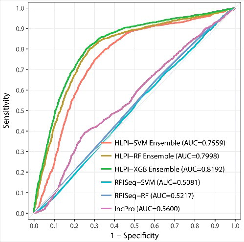
In Fig. 1, we can see that the AUC values of HLPI-SVM Ensemble, HLI-RF Ensemble, HLPI-XGB Ensemble, RPISeq-SVM, RPISeq-RF and lncPro are 0.7559, 0.7998, 0.8192, 0.5081, 0.5217 and 0.5600 respectively. It is clear that the AUCs of the HLPI-Ensemle models are much higher than other similar prediction methods in the lncRNome dataset. Unfortunately, RPI-Pred only provide the results of the binary classification format, so we cannot draw its ROC curve. We convert the result of the probability format provided by RPIPred, lncPro, RPISeq-SVM, RPISeq-RF into a binary classification format with 0.5 as the boundary. Furthermore, we specified that probability value greater than 0.5 as positive and the probability less than 0.5 as negative [15]. Based on these binary classification results, we calculate all the indicators of HLPI-Ensemble and other models (see Table 5).

Table 5. The performance of HLPI-Ensemble, RPI-Pred, lncPro, RPISeq-SVM and RPISeq-RF in lncRNome database.

Model	AUC	ACC	REC	SPEC	PPV	F1 score	TP	FN	FP	TN
HLPI SVM-Ensemble	0.7559	0.7039	0.8805	0.5272	0.6506	0.7483	2403	326	1290	1439
HLPI RF-Ensemble	0.7998	0.6844	0.8995	0.4694	0.6290	0.7403	2455	274	1448	1281
HLPI XGB-Ensemble	0.8192	0.7643	0.8292	0.6995	0.7340	0.7787	2263	466	820	1909
RPI-Pred	—	0.4541	0.8732	0.0351	0.4750	0.6153	2383	346	2633	96
RPISeq-SVM	0.5081	0.0218	0.8534	0.1623	0.5046	0.6342	2329	400	2286	443
RPISeq-RF	0.5217	0.5027	0.9849	0.0205	0.5013	0.6645	2688	41	2673	56
lncPro	0.5600	0.5271	0.8490	0.2052	0.5164	0.6422	2317	412	2169	560

As shown in Table 5, the three ensemble models of HLPI-Ensemble are better when compared to the other methods, which indicate HLPI-Ensemble has an excellent advantage in predicting human lncRNA-protein interactions. Furthermore, we find that all models except HLPI-ensemble models have high false positive problems. It can be seen from FP that the previous models are biased toward predicting the unknown lncRNA-protein pairs as positive. In addition, the extreme imbalance between REC and SPEC also show that there is high false positive risk in previous models. The high FP is the main reason for the poor prediction performance. Compared to the previous models, the three HLPI-Ensemble models have been greatly improved in reducing false positives. The REC and SPEC of the HLPI-Ensemble models are better than the previous models. Further, the AUC of HLPI-Ensemble models surpassed all previous models, which suggest that HLPI-Ensemble models have strong applicability in predicting potential human lncRNA-protein interactions. In addition, other indicators of HLPI-Ensemble models are higher than the previous models, which further show the superiority of the ensemble strategy. In short, the results of the external validation confirm the robustness of the ensemble strategy and the practical value of HLPI-Ensemble in predicting human lncRNA-protein interactions.

Discussion

The reasons for the success of HLPI-Ensemble may come from the following factors. First, the HLPI-Ensemble is specially designed for human lncRNA-protein interactions prediction. None of the previous models distinguish the sources of RNA. They try to build a model that can predict the RNA-protein association of all species. Unlike the previous models, HLPI-Ensemble focuses on human lncRNA-protein interactions prediction. The 8120 experimental validation of human lncRNA-protein interactions are extracted from NPInter for constructing HLPI-Ensemble. Furthermore, we apply three types of feature extraction algorithms for lncRNA and protein, respectively, which produce nine types of combinations of features. These nine types of combination features summarize the association between human lncRNA and protein. Compared with the previous model, HLPI-Ensemble have a stronger specificity in predicting human lncRNA-protein.

Second, the ensemble strategy and the random pairing strategy is applied to effectively reduce false positive rate. As shown in the external validation, previous models predict most human lncRNA-protein interactions as positive. The reason for the high false positivity may be the negative sample selection of the previous models. Most of the previous models chose RNA that could not bind to proteins and protein that could not bind to RNAs as negative sample. Biology researchers, however, are more concerned with the interactions between RNA capable of binding proteins and RNA binding proteins, which are different from the negative samples of previous models. This results in high false positive of the previous models. HLPI-Ensemble is different from the previous models, since it introduces the random pairing strategy to generate negative samples. The positive samples of HLPI-Ensemble are experimentally confirmed interaction pairs of lncRNA and protein. Although the negative samples provided by the random matching strategy are not necessarily accurate, they can effectively reduce the risk of false positives. Compared with the negative results, the researchers are more concerned with the positive results. The false positive results will lead to the waste of experimental resources or even misleading research. HLPI-Ensemble can help researchers keep away from false positives and correctly predict unknown human lncRNA-protein relationships. Finally, the ensemble strategy improves the performance of the overall model. It can be seen from Table 3 and Table 4 that most HLPI-Ensemble models perform better than their corresponding sub-models. Although the sub-model from Table 3 also has a false positive problem, it can be seen from the comparison between Table 3 and Table 4 that the FP of all HLPI-Ensemble models are significantly lower than the corresponding sub-models. This suggests that the ensemble strategy can effectively reduce the false positive. Because the ensemble strategy integrates the advantages of sub-models trained by different feature combinations, the ensemble models performs better than the previous single models. In summary, compared to the previous models, HLPI-Ensemble has good robustness in the prediction of human lncRNA-protein interactions.

Of course, HLPI-Ensemble have some limitations that need to be improved in the future. For example, the known human lncRNA-protein interactions data is still insufficient. More human lncRNA-protein interactions data can further improve the performance of HLPI-Ensemble. In addition, ensemble strategy is based on multiple sub-models, which results in huge computational resources. As the level of hardware continues to raise the problem will be resolved.

To help researchers further study human lncRNA-protein interactions, we create a free website for HLPI-Ensemble (http://ccsipb.lnu.edu.cn/hlpiensemble/). In addition, people can download all the datasets of this study from the web site. It should be noted that HLPI-Ensemble is designed to predict human lncRNA-protein interactions, which does not support lncRNA data and protein data from other species.

Materials and methods

Dataset

We apply the NPInter v2.0 database [30] as the benchmark dataset and the lncRNome database [29] is applied as the external validation dataset. The construction of these two datasets is shown below.

Benchmark dataset

The data extracted to construct HLPI-Ensemble come from the NPInter v2.0 database [30]. NPInter is a database that integrated the experimental interactions of ncRNA and multiple biomolecules. NPInter covers the majority of known human lncRNA-protein interactions. Fig. 2 shows the process of constructing benchmark dataset from NPInter v2.0.

Figure 2. The process of constructing benchmark dataset.

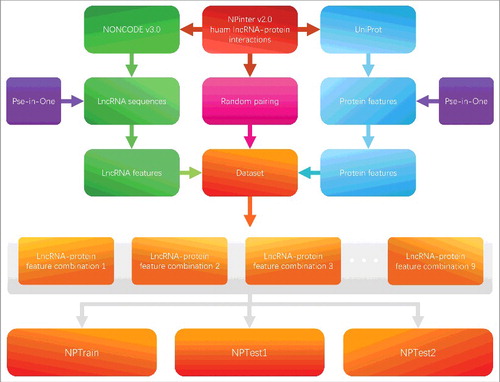
As shown in Fig. 2, the human lncRNA-protein interactions are extracted from NPInter v2.0 database. The process of filtering and cleaning data is strictly based on three principles. First, the species of the lncRNA-protein entity must be human. Second, the lncRNA-protein interaction type must be “binding.” Finally, the entity must have a Pubmed ID that can be queried, meaning that the entity can be experimentally tested. After data cleaning, we obtain 8120 experimental validated human lncRNA-protein interactions data. The lncRNA data of NPInter is extracted from the NONCODE v3.0 database [31]. The NONCODE database provides a most complete collection and annotation of lncRNA. The protein data of NPInter is extracted from the UniProt database [32]. UniProt covers almost all known protein information. We extract lncRNA sequences and protein sequences from NONCODE and UniProt, respectively. Next, the lncRNA features and protein features are extracted from lncRNA sequences and protein sequences by Pse-in-One, respectively. At the same time, the random pairing strategy is applied to generate negative samples according to the known human lncRNA-protein interactions. In the random pairing strategy, the experimentally validated lncRNA and protein interactions pairs are disrupted and randomly paired. Then, the random matched interactions pairs that duplicate with positive samples (known interactions pairs) are removed. The remaining random pairs are treated as the negative dataset. To ensure the data balance, the sample size of the negative dataset generated by the random pairing strategy is equal to the sample size of the positive dataset. Finally, we equally divide the data into three divisions which are NPTrain, NPTest1, and NPTest2. Among them, NPTrain is the training dataset. NPTest1 is used to test the performance of the sub-models. NPTest2 is used to compare the performance of different ensemble strategies.

External validation dataset

The dataset implemented by external validation is extracted from the lncRNome database [29]. The lncRNome database is a comprehensive knowledge base for human lncRNA. The process of generating external validation dataset is similar to the process of generating benchmark dataset. Further, we remove the overlap between lncRNome and NPInter v2.0. First, we have executed a crawler script written by ourselves to get the human lncRNA-protein entity in lncRNome database. Next, we get the lncRNA's corresponding entity in NPInter v2.0 database based on the conversion of the Ensemble ID stored by lncRNome database through the NONCODE database. These lncRNome entities that can be converted to NPInter entities are overlapping data. The overlapped data is removed to ensure the reliability and fairness of the test results. In addition, some of the lncRNome entity is incomplete, such as the lack of Ensemble ID or the lack of sequence information. These lncRNome entities are invalid and they can neither be used for building models nor used to evaluate models. Obviously, such invalid data must also be removed. After filtering out the invalid data, we extracted 2729 pairs of human lncRNA-protein interaction from lncRNome and generated 2729 negative samples by application random pairing strategy.

Data features

The data features are generated by Pse-in-One. The Pse-in-One is a popular feature extraction model that extracts the features of DNA, RNA, and protein by pseudo components [33]. We utilize Pse-in-One to extract lncRNA features and protein features. The features of lncRNA and protein are matched to produce nine types of feature combinations for sub-models training. The process of lncRNA feature and protein feature extraction is described in the following paragraphs. For details, see Supplementary Materials 1.

LncRNA features

A variety of feature extraction methods are integrated in Pse-in-One. We apply three types of them, including Kmer, DAC, and PC-PseDNC-General. In these methods, Kmer is the simplest method of representing lncRNA. Kmer represents the frequency of occurrence of k adjacent nucleic acids by lncRNA sequence [34]. A total of 16 lncRNA features are extracted by Kmer. Another algorithm for generating lncRNA features is Dinucleotide-based auto covariance (DAC) [35, 36]. The DAC measures the correlation of same physicochemical index between two dinucleotides separated by a distance of lag along the lncRNA sequence. We extracted 44 lncRNA features from the DAC. The last algorithm for generating lncRNA characteristics is the general parallel correlation pseudo dinucleotide composition (PC-PseDNC-General) [37]. Pseudo dinucleotide composition is a class of common feature extraction algorithm for nucleic acid sequences, which is based on nucleic acid sequence of various physiochemical indices. We extracted 22 physiochemical indices built in PC-PseDNC-General as lncRNA features.

Protein features

The process of generating protein features is similar to the process of generating lncRNA features. We apply three types of protein sequence feature extraction methods of Kmer, AC and PC-PseAAC-General. The principle of the Kmer algorithm is not repeated here as described above [34]. A total of 400 protein features are extracted by Kmer. The AC approach measures the correlation of same property between two residues separated by a distance of lag along the protein sequence [38]. We extracte 1094 protein features from the AC. General parallel correlation pseudo amino acid composition (PC-PseAAC-General) is a feature extraction algorithm for measuring the physicochemical properties of amino acid sequences [38]. We extract 22 protein features from PC-PseAAC-General based on the default parameters of Pse-in-One.

Ensemble model

The performance of a single predictive model is limited by the features of the model and its own predictive ability. Applying ensemble strategies with multiple single models can improve the overall performance of model. In addition, the ensemble model covers a wide range of features that are more robust than a single model. Here, we introduce the average ensemble strategy and the linear ensemble strategy to further improve the model performance. HLPI-Ensemble employs three machine algorithms of Support Vector Machines (SVM), Random Forests (RF) and Extreme Gradient Boosting (XGB) to implement the ensemble strategy to construct HLPI-SVM Ensemble, HLPI-RF Ensemble and HLPI-XGB Ensemble. Fig. 3 shows the process of the ensemble strategy implemented in these three models.

Figure 3. The construction process of HLPI-Ensemble model.

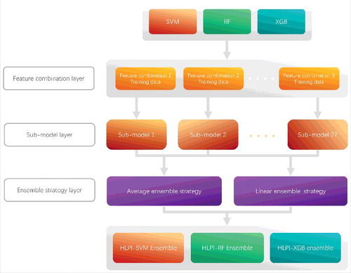
As shown in Fig. 3, the HLPI-Ensemble consists of three parts: Feature combination layer, Sub-model layer and Ensemble strategy layer. First, three lncRNA feature data and three protein feature data are combined in the Feature combination layer. A total of nine types of feature combinations are generated. Next, three types of machine learning algorithms of SVM, RF and XGB are trained by nine types of feature combinations, respectively. A total of 27 sub-models are generated in the Sub-model layer. Finally, we choose an ensemble strategy for corresponding HLPI-Ensemble model from the average ensemble strategy and the linear ensemble strategy according to the performance of ensemble strategy in the Ensemble strategy layer.

Then, we apply the 10-fold cross-validation (10-fold CV) to test the performance of models. 10-fold CV is an evaluation method for the binary class model. It randomly divides the data set into 10 parts and then uses nine of these data to train model, with the remaining one as the test set. Repeat this process to ensure that each part has been served as test set. Finally, take an average of 10 prediction results as the final result of evaluation. In addition, we also apply the 10-fold CV in the parameter tuning process. However, the results of 10-fold CV are contingent. In order to obtain stable results, we repeat this process 100 times in all 10-fold CV.

Sub-model and tuning parameters

HLPI-Ensemble consists of HLPI-SVM Ensemble, HLPI-RF Ensemble and HLPI-XGB Ensemble. Each class of ensemble model is supported by nine types of sub-models. All sub-model parameters are optimized.

The sub-models of HLPI-SVM Ensemble are based on the SVM algorithm. The core idea of SVM is to construct hyperplanes or a set of hyperplanes in high or infinite dimensional spaces that can be used for classification, regression, or other tasks [16]. The sub-models of HLPI-SVM Ensemble employ Radial Basis Function Kernel as core. In addition, random search is applied to tune parameters. Further, the tuned parameters of each model are verified by 100 times 10-fold CV to ensure the reliability of the results. The parameter with the highest AUC value is chosen as the final parameter of the sub-model. All the sub-models of HLPI-SVM Ensemble have applied the above optimization process.

The sub-models of HLPI-RF Ensemble are based on the RF algorithm. RF is a classifier that uses multiple decision trees to train and predict samples [17]. The parameter tuning process of HLPI-RF Ensemble sub-model is similar to the process of HLPI-SVM Ensemble sub-model. The difference is that the HLPI-RF Ensemble sub-model applies the grid search to find the optimal combination of parameters. Each parameter's model is validated by 100 times 10-fold CV. The combination of the parameters with the highest AUC value is chosen as the final parameter of the sub-model. All sub-models of HLPI-RF Ensemble had applied the above optimization process.

The sub-model of HLPI-XGB Ensemble is based on the XGB algorithm. XGB is a popular algorithm in recent years, it has improved Gradient boosting algorithm and achieved a good performance improvement [23, 39]. The XGB algorithm has several parameters that need to be adjusted. Traversing all combinations of parameters takes a lot of computational time. In order to shorten the search time, fixed parameter techniques are used to quickly narrow the search range of parameters. First, the XGB hyperparameters are initially set based on our past modeling experience. Then, the grid search is used to find the optimal value of the first parameter while the other parameters remain fixed. All search results were validated by 3 times 10-fold CVs. When the optimal value of the first parameter is found, replace the first argument with the grid search result. The process of searching for the second parameter is similar to the above procedure. When all the parameters have found the optimal solution, the process of search is stopped. Finally, we would get a collection containing all the optimal parameters. However, the parametric combination of fixed parameter techniques may not be a globally optimal solution. In order to further enhance the reliability of the model parameters, we carry out grid search within the optimized parameters. In this process, all the results were verified by 100 times10-fold CV. The combination of the parameters with the highest AUC value is chosen as the formal parameter of the sub-model. All sub-models of HLPI-XGB Ensemble have applied the above optimization process.

Ensemble strategy

HLPI-Ensemble introduces the average ensemble strategy and linear integration strategy, which are applied to generate HLPI-SVM Ensemble, HLPI-RF Ensemble and HLPI-XGB Ensemble.

The core idea of the average ensemble strategy is to average the prediction results of sub-models as the final results. The average ensemble strategy is defined as follows.

$AVG =\frac{{{\displaystyle \sum }}_i^n{X}_i}{n}$

In the above formula, n represents the number of integrated sub-models, $X_i$ represents the prediction result of the i-th sub-model. The prediction result of the sub-model is the probability of interaction between each lncRNA-protein pair. The advantage of the average ensemble strategy is that it reduces the influence of the anomalous results on the overall prediction results to further improve the robustness of the ensemble model. Taking HLPI-SVM Ensemble as an example. HLPI-SVM Ensemble covers nine types of sub-models and their corresponding feature combinations are different. Different combinations of features tend to different predictions. Assuming that the nine types of sub-models predict a pair of unknown human lncRNA-protein interactions and their results are 0.96, 0.90, 0.88, 0.20, 0.86, 0.88, 0.92, 0.89, 0.96. It can clearly see that 0.20 is anomalous in these values. Abandoning 0.20 is unwise because it may imply factors that ignored by other sub-models. The contribution of each sub-model should be considered. The average ensemble strategy is applied to the above prediction results, and the final prediction result is 0.83, which is close to the prediction results of all sub-models.

Another ensemble strategy for HLPI-Ensemble is linear ensemble, which integrated sub-models based on linear model algorithms. The linear integration strategy applies the multivariable linear regression model (MLRM). The linear ensemble strategy is defined as follows.

$Y ={\beta }_0 +{\beta }_1{X}_1+{\beta }_2{X}_2+{\beta }_i{X}_i+···+{\beta }_n{X}_n$

In the above formula, n represents the number of integrated sub-models, $\beta$ denotes the model coefficients, $X_i$ represents the prediction probability result of the i-th sub-model, $Y$ denotes the prediction result of the linear ensemble strategy. MLRM take the NPTest1 prediction results of all sub-model as training dataset. Table 6 shows the coefficients of each HLPI-Ensemble model trained by linear ensemble strategy.

Table 6. The coefficients of HLPI-Ensemble models trained by linear ensemble strategy.

HLPI-Ensemble model	${\beta }_0$	${\beta }_1$	${\beta }_2$	${\beta }_3$	${\beta }_4$	${\beta }_5$	${\beta }_6$	${\beta }_7$	${\beta }_8$	${\beta }_9$
HLPI-SVM Ensemble	4.206	−0.497	−1.095	−1.844	−8.087	6.045	−2.911	14.73	−12.53	−1.164
HLPI-RF Ensemble	4.352	6.161	−3.442	−4.094	−2.732	2.522	−4.186	7.761	−3.863	−6.288
HLPI-XGB Ensemble	4.328	0.5581	0.3794	−1.700	0.0096	−1.247	−3.704	1.295	−2.886	−0.1375

From Table 6 we can see that the assigned weights of the sub-models are different. The linear ensemble strategy tends to assign different weights to the different sub-models. As can be seen from Table 6, ${\beta }_7$ is the largest coefficient in HLPI-SVM Ensemble. This suggests that the ${\beta }_7$-related HLPI-SVM Ensemble sub-model contributes the most to HLPI-SVM Ensemble. Similarly, ${\beta }_7$ in HLPI-RF Ensemble also has the same interpretation. In HLPI-Ensemble XGB, ${\beta }_6$ has the largest absolute value of all coefficients.

Disclosure of potential conflicts of interest

No potential conflicts of interest were disclosed.

Acknowledgment

This work was supported by the National Natural Science Foundation of China under Grant No. 31570160, Innovation Team Project of Education Department of Liaoning Province under Grant No. LT2015011, the Doctor Startup Foundation from Liaoning Province under Grant No. 20170520217, Important Scientific and Technical Achievements Transformation Project under Grant No. Z17-5-078, Large-scale Equipment Shared Services Project under Grant No. F15165400 and Applied Basic Research Project under Grant No. F16205151.

Additional information

Funding

This work was supported by the Doctor Startup Foundation from Liaoning Province, 20170520217; Innovation Team Project of Education Department of Liaoning Province, LT2015011; Large-scale Equipment Shared Services Project, F15165400; Important Scientific and Technical Achievements Transformation Project, Z17-5-078; Applied Basic Research Key Project of Yunnan, F16205151; National Natural Science Foundation of China, 31570160 and 61772531.

References

- UA Ø, Derrien T, Beringer M, et al. Long noncoding RNAs with enhancer-like function in human cells. Medecine Sciences M/s. 2010;143(1):46–58.
- Guttman M, Amit I, Garber M, et al. Chromatin signature reveals over a thousand highly conserved large non-coding RNAs in mammals. Nature. 2009;458(7235):223.
- Crick FHC, Barnett L, Brenner S, et al. General Nature of the Genetic Code for Proteins. Nature. 1961;192(4809):1227–1232.
- Yanofsky C. Establishing the triplet nature of the genetic code. Cell. 2007;128(5):815–8.
- Bertone P, Stolc V, Royce TE, et al. Global identification of human transcribed sequences with genome tiling arrays. Science. 2004;306(5705):2242.
- Chen X. Predicting lncRNA-disease associations and constructing lncRNA functional similarity network based on the information of miRNA. Sci Rep. 2015;5:13186.
- Consortium EP, Birney E, Stamatoyannopoulos JA, et al. Identification and analysis of functional elements in 1% of the human genome by the ENCODE pilot project. Nature. 2007;447(7146):799–816.
- Carninci P, Sandelin A, Lenhard B, et al. Genome-wide analysis of mammalian promoter architecture and evolution. Nat Genet. 2006;38(6):626–35.
- Chen X, You ZH, Yan GY, et al. IRWRLDA: improved random walk with restart for lncRNA-disease association prediction. Oncotarget. 2016;7(36):57919.
- Chen X. KATZLDA: KATZ measure for the lncRNA-disease association prediction. Sci Rep. 2015;5:16840.
- Chen X, Huang YA, Wang XS, et al. FMLNCSIM: fuzzy measure-based lncRNA functional similarity calculation model. Oncotarget. 2016;7(29):45948–45958.
- Huang YA, Chen X, You ZH, et al. ILNCSIM: improved lncRNA functional similarity calculation model. Oncotarget. 2016;7(18):25902–25914.
- Moran VA, Niland CN, Khalil AM. Co-Immunoprecipitation of long noncoding RNAs. Methods Mol Biol. 2012;925(925):219.
- Bellucci M, Agostini F, Masin M, et al. Predicting protein associations with long noncoding RNAs. Nat Methods. 2011;8(6):444.
- Muppirala UK, Honavar VG, Dobbs D. Predicting RNA-Protein Interactions Using Only Sequence Information. Bmc Bioinformatics. 2011;12(1):489.
- Cortes C, Vapnik V. Support Vector Network. 1995;20(3):273–297.
- Ho TK. The Random Subspace Method for Constructing Decision Forests. IEEE Transactions on Pattern Analysis & Machine Intelligence. 1998;20(8):832–844.
- Wang Y, Chen X, Liu ZP, et al. De novo prediction of RNA–protein interactions from sequence information. Molecular Biosystems. 2013;9(1):133.
- Lu Q, Ren S, Lu M, et al. Computational prediction of associations between long non-coding RNAs and proteins. Bmc Genomics. 2013;14(1):651.
- Suresh V, Liu L, Adjeroh D, et al. RPI-Pred: predicting ncRNA-protein interaction using sequence and structural information. Nucleic Acids Res. 2015;43(3):1370.
- Ge M, Li A, Wang M. A Bipartite Network-based Method for Prediction of Long Non-coding RNA-protein Interactions. Genomics Proteomics Bioinformatics. 2016;14(1):62–71.
- Pan X, Fan Y, Yan J, et al. IPMiner: hidden ncRNA-protein interaction sequential pattern mining with stacked autoencoder for accurate computational prediction. BMC Genomics. 2016;17:582.
- Chen T, Guestrin C. editors. XGBoost:A Scalable Tree Boosting System. ACM SIGKDD International Conference on Knowledge Discovery and Data Mining. 2016.
- Ling CX, Huang J, Zhang H. editors. AUC: A Better Measure than Accuracy in Comparing Learning Algorithms. Canadian Society for Computational Studies of Intelligence Conference on Advances in Artificial Intelligence. 2003.
- Fawcett T. An introduction to ROC analysis. Pattern Recognition Letters. 2006;27(8):861–874.
- Diebold FX, Mariano RS. Comparing Predictive Accuracy. Nber Technical Working Papers. 1995;13(3):253–263.
- Powers DMW. Evaluation: From Precision, Recall and F-Factor to ROC, Informedness, Markedness & Correlation. Journal of Machine Learning Technologies. 2011;2:2229–3981.
- Li Z, Ai H, Wen C, et al. CarcinoPred-EL: Novel models for predicting the carcinogenicity of chemicals using molecular fingerprints and ensemble learning methods. Sci Rep. 2017;7(1):2118.
- Bhartiya D, Pal K, Ghosh S, et al. lncRNome: a comprehensive knowledgebase of human long noncoding RNAs. Database, 2013,(2013-01-01). 2013;2013(14):bat034.
- Yuan J, Wu W, Xie C, et al. NPInter v2.0: an updated database of ncRNA interactions. Nucleic Acids Res. 2014;42(Database issue):104–8.
- Bu D, Yu K, Sun S, et al. NONCODE v3.0: integrative annotation of long noncoding RNAs. Nucleic Acids Res. 2012;40(Database issue):210–5.
- Gane PJ, Bateman A, Mj M, et al. UniProt: A hub for protein information. Nucleic Acids Res. 2015;43(Database issue):204–12.
- Liu B, Liu F, Wang X, et al. Pse-in-One: a web server for generating various modes of pseudo components of DNA, RNA, and protein sequences. Nucleic Acids Res. 2015;43(Web Server issue):W65–W71.
- Wei L, Liao M, Gao Y, et al. Improved and Promising Identification of Human MicroRNAs by Incorporating a High-Quality Negative Set. IEEE/ACM transactions on computational biology and bioinformatics. 2014;11(1):192–201.
- Dong Q, Zhou S, Guan J. A new taxonomy-based protein fold recognition approach based on autocross-covariance transformation. Bioinformatics (Oxford, England). 2009 Oct 15;25(20):2655–62.
- Guo Y, Yu L, Wen Z, et al. Using support vector machine combined with auto covariance to predict protein-protein interactions from protein sequences. Nucleic Acids Res. 2008 May;36(9):3025–30.
- Chen W, Zhang X, Brooker J, et al. PseKNC-General: a cross-platform package for generating various modes of pseudo nucleotide compositions. Bioinformatics (Oxford, England). 2015;31(1):119–20.
- Cao DS, Xu QS, Liang YZ. Propy: a tool to generate various modes of Chou's PseAAC. Bioinformatics (Oxford, England). 2013;29(7):960–2.
- Efron B, Hastie T, Johnstone I, et al. Least Angle Regression. Annals of Statistics. 2004;32(2): págs. 407–451.