Deep learning identifies genome-wide DNA binding sites of long noncoding RNAs

ABSTRACT

Long noncoding RNAs (lncRNAs) can exert their function by interacting with the DNA via triplex structure formation. Even though this has been validated with a handful of experiments, a genome-wide analysis of lncRNA-DNA binding is needed. In this paper, we develop and interpret deep learning models that predict the genome-wide binding sites deciphered by ChIRP-Seq experiments of 12 different lncRNAs. Among the several deep learning architectures tested, a simple architecture consisting of two convolutional neural network layers performed the best suggesting local sequence patterns as determinants of the interaction. Further interpretation of the kernels in the model revealed that these local sequence patterns form triplex structures with the corresponding lncRNAs. We uncovered several novel triplexes forming domains (TFDs) of these 12 lncRNAs and previously experimentally verified TFDs of lncRNAs HOTAIR and MEG3. We experimentally verified such two novel TFDs of lncRNAs HOTAIR and TUG1 predicted by our method (but previously unreported) using Electrophoretic mobility shift assays. In conclusion, we show that simple deep learning architecture can accurately predict genome-wide binding sites of lncRNAs and interpretation of the models suggest RNA:DNA:DNA triplex formation as a viable mechanism underlying lncRNA-DNA interactions at genome-wide level.

KEYWORDS:

• Long noncoding RNAs
• deep learning
• triplex

Introduction

There has been increasing evidence that long noncoding RNAs (lncRNAs) regulate biological processes via different mechanisms [1–4] including RNA-protein interactions, as well as RNA-RNA interactions and RNA-DNA interactions. Such interactions are important for the proper organization of the chromatin and regulation of associated genes. In this study, we focus on developing and interpreting computational model that can predict DNA-lncRNA interactions. which can contribute to proper chromatin organization and regulate expression of nearby genes.

There have been a few studies that indicate that DNA-lncRNA interactions happen via RNA-DNA triplex formation with experimental validation of a handful of interactions for lncRNAs such as HOTAIR [5], MEG3 [6], and TUG1 [7]. A genome-wide analysis to interpret DNA-lncRNA interactions will provide further insights to this mechanism. Using Chirp-Seq (or Chromatin Isolation by RNA purification) technique, extraction of regions of genome bound by different lncRNAs have been possible [8–10]. The sequences representing these regions can be analyzed for corresponding lncRNAs to test if RNA-DNA triplex formation is a viable mechanism that drives DNA-lncRNA interactions. We aim to use predictive models to predict sequences that interact with a particular lncRNA and test the performance using the sites obtained by ChIRP-Seq experiments.

Recently, deep learning models such as deep convolutional neural networks (CNN) [11,12] have been successfully applied to sequence-based problems in genomics signals . For example, DeepBind [13] and DeepSEA [14] have been successfully applied deep learning to predict the DNA-protein interactions in high-throughput ChIP-Seq data produced by the Encyclopedia of DNA Elements (ENCODE) project. Another form of deep learning model recurrent neural network (RNN) has also been applied in problems related to protein structure prediction, classification, and gene expression regulation. In general, a CNN layer captures local patterns while a RNN layer captures long range patterns or dependencies. Since, there is no clear evidence on what kind of deep learning architecture best explains DNA-lncRNA interactions, we explore different architectures of convolutional neural networks and recurrent neural networks to model DNA sequences which interact with a given lncRNA.

To perform the analysis, we compiled a comprehensive set of genome-wide binding sites of 12 different lncRNAs from publicly available ChIPR-Seq peaks. We show that compared to recurrent neural networks, simpler architectures with only two convolutional layers in deep learning model can accurately predict genome-wide lncRNA binding peaks uncovered by ChIPR-Seq experiments. This suggests local sequence patterns as determinants for positive cases of interactions between DNA and lncRNAs. The performance of the CNN models also increased with increase in number of kernels used. We found that majority of the subsequences within the ChIPR-Seq peaks which best represent the kernels in the first CNN layer form triplex structures with their respective lncRNAs suggesting RNA:DNA:DNA triplex formation as the underlying mechanism. Unlike the usual method of directly predicting the triplex forming domains (TFDs) of a lncRNA by using Triplexator, we uncovered TFDs of 12 lncRNA by mapping the portions of the lncRNA sequence which formed triplex structures only with these subsequences. Some of the experimentally verified TFDs of lncRNAs such as HOTAIR and MEG3 were detected in this paper. TFDs which were not previously reported were also detected in this paper. We experimentally verified such two TFDs of lncRNAs HOTAIR and TUG1 predicted by our method (but previously unreported) using Electrophoretic mobility shift assays. In conclusion, we show that simple deep learning architecture can accurately predict genome-wide binding sites of lncRNAs and further interpretation of the models suggest RNA:DNA:DNA triplex formation as a viable mechanism underlying lncRNA interactions with DNA at genome-wide level.

Materials and methods

ChIRP-Seq data

We collected coordinates of genome-wide Chirp-Seq peaks of 12 lncRNAs (8 mouse, 3 human, and 1 fruit fly) from publicly accessible NCBI GEO repository (Table 1).

Table 1. Chirp-Seq data set used in this paper. The table shows number of peaks obtained from ChIRP-Seq of 12 lncRNAs. Genome and GEO accession number are also shown for each ChIRP-Seq data set.

LncRNA	Number of ChIRP-Seq Peaks	GEO accession number	Genome
lincHSC2	264	GSE66819	Mouse
EC7	268	GSE97119	Mouse
ROX2	307	GSE31332	Drosophila
HOTAIR	832	GSE31332	Human
RMRP	2002	GSE73912	Mouse
TERC	2198	GSE31332	Human
HOTCHON (Limb)	2880	GSE70986	Mouse
HOTCHON (Glial)	2919	GSE70986	Mouse
MEG3	9010	GSE99798	Mouse
LIN28	32387	GSE90574	Mouse
DACOR1	40300	GSE58989	Human
PANCT1	43581	GSE73805	Mouse
TUG1	130269	GSE77493	Mouse

Training, testing and data augmentation

50% of the peaks were used for training, 25% were used for validation set, and remaining 25% for testing purposes. lncRNAs with less than 500 ChIRP-Seq peaks, data augmentation was applied to increase the size of the training set by randomly shifting each binding peak left or right with base pairs between 10 and 40. This was repeated four times for each binding site. While it was repeated two times for each binding intervals in cases of lncRNAs with less than 10,000 but more than 500 Chirp-Seq peaks. The sequences corresponding to these augmented training set served as the positive cases of lncRNA binding sites. To generate the negative binding cases, sequences of similar lengths were randomly selected from the genome using bedtools excluding the regions occupied by peaks. We used this technique instead of shuffling the positive sequence because the later approach can lead to overestimated performance [15]. Similarly, negative instances in the testing set were generated randomly from the genome. To remove redundancy between training and testing set, sequences in testing set which are at least 90% similar to sequence in training set were removed using CD-HIT (http://weizhongli-lab.org/cd-hit/).

Input layer

In our case, DNA sequences represent the input data and the goal is to predict if a lncRNA will interact with it (class label +1) or not (class label −1). The raw nucleotide characters (A, C, G, T) in the sequence were used as inputs, where they were converted into a one hot encoding (a binary vector with the matching character entry being a 1 and the rest as 0s). This encoding matrix is used as the input layer to the deep learning models that performs the prediction (Fig. 1).

Figure 1. Convolutional neural network and recurrent neural network layers. (A) Illustration of CNN model with the input layer (sequence) as one-hot encoded followed by a CNN layer followed by a global max pooling layer and output layer with a single node with sigmoid activation function. (B) Illustration of a RNN model with the input layer (sequence) as one-hot encoded followed by a concatenated bidirectional LSTM layer followed by an output layer with single node with sigmoid activation.

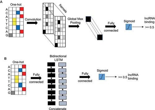
Convolutional and pooling layer

Convolutional neural network (CNN), when applied in the context of DNA sequences, can learn local sequence patterns or ‘motifs’ which are good discriminators between the positive and negative instances in the training set. The information of the motifs is embedded in the entries of a kernels (filters) used in the first convolution layer. Additional CNN layers can learn higher order interaction between those motifs. A convolution filter or kernel of size k takes an input data matrix X of size T x N_in, with length T and input layer size N_in, and outputs a matrix Z of size T x N_out, where N_out is the output layer size. We used rectified linear units (ReLU) as the nonlinear activation function in the neurons. After the convolution, a pooling layer is usually applied to reduce the size of the output matrix from the CNN layer. Figure 1A shows a CNN model with one single convolutional layer. In this model, a global-max pooling layer is used after the convolution layer because it has been shown to be the most appropriate pooling technique for genomic signals [16].The output of the pooling layer is fed to the output softmax layer for classification.

Recurrent layer

Recurrent neural networks (RNNs) have become the main neural network to handle sequential data. Given an input matrix X of size T x N_in, an RNN layer produces matrix H of size T x d, d is the RNN embedding size. At each time step t, an RNN takes an input column vector x_t of length N_in and the output of length from previous hidden neuron and produces output (which acts an input to then next hidden neuron). We used an RNN variant called the Long Short-term Memory (LSTM) layer, which can handle long term dependencies using gating functions. RNNs generate an output vector at each time step of the input sequence. For classification purpose, we used the average of all the vectors and the used the mean vector as the input to the final output softmax layer. We used a bi-directional LSTM layer in which the input sequence goes through two LSTM networks, in forward and backward directions. These two networks produce two matrices, each containing column vectors representing the time steps. These vectors are averaged to create one vector for each direction. The forward and backward vectors are concatenated and act as the input to the final output softmax layer. Figure 1B shows a RNN model with one single LSTM layer.

Models

In our study, we tried several versions of CNN models by varying the number of layers and kernels, but here we report 15 of them which performed the best. 16_miniCNN, 32_miniCNN, and 64_miniCNN models had one hot encoded input layer representing the training sequences followed by one hidden CNN layer with 16, 32, and 64 kernels, respectively. The ReLU activation function was used. The CNN layer was followed by a global max pooling layer (local pooling was attempted but performed poorly). Finally, the output of the pooling layer was connected to the ouput layer with one single neuron which the Sigmoid activation function. 16_smallCNN, 32_smallCNN, and 64_smallCNN models had one input layer followed by two hidden CNN layers with 16, 32, and 64 kernels, respectively. The ReLU activation function was used in each hidden layer. The first CNN layer was followed by a local max pooling layer (with pooling size of 10 bases and stride size of 5 bases). The second CNN layer was followed by a global max pooling layer. Similarly, mediumCNN, largeCNN and verylargeCNN models containing 3, 4, and 5 CNN layers, respectively were also tested. Three different number of kernels (16, 32, and 64) in the CNN layer in each of three models were tested. The size of each kernel or filter was 15 × 1 in all the 15 CNN models. 15 base pairs were long enough to capture the short sequence motifs in the positive DNA sequences that differentiate them from the negative sequences. To prevent overfitting, we added dropout layer and batch normalization layer after the every hidden CNN layers models. Dropout percentage was set to 20% for first CNN layer and it was set to 30% for second or subsequence CNN layers)

Three Recurrent Neural Network (RNN) models (15_smallRNN, 5_smallRNN, and 30_smallRNN) were tested. Each model had one bidirectional LSTM layer each of sizes 15, 5, and 30, respectively. The LSTM layer was made bidirectional and hence it sweeps from left to right and right to left. The output from the LSTM layer was a vector (output at each ‘time step’) of each direction were concatenated and averaged before feeding as input to the final output layer. To prevent overfitting, a dropout layer (dropping 30% of nodes) was used.

The output layer contained a single neuron with Sigmoid activation function, which learns the mapping from the hidden layers to the output class labels [+1, −1]. The final output is a probability indicating whether an input is a positive or a negative binding site (binary classification task).

Training

The parameters of the network were trained end-to-end by minimizing the binary cross-entropy over the training set. The minimization of the loss function was obtained via the stochastic gradient algorithm Adam, with a mini-batch size of 50 sequences. Three different learning rates (0.001, 0.005, 0.05) were tested. The training phase was set for 150 epochs but early stopping criteria on the optimization procedure was used when the value of the loss function on the validation set stop decreasing for 11 consecutive epochs. Six different metrics (accuracy, area under the curve, F1 score, MCC or Matthews correlation coefficient, Precision, and Recall) were used to evaluate the performance of the models.

Results

Data preparation before model tuning

We collected coordinates of genome-wide Chirp-Seq peaks of 12 different lncRNAs (8 mouse, 3 human, and 1 fruit fly) from publicly accessible NCBI GEO repository (Table 2). The number of Chirp-Seq peaks varied from few hundreds (lncRNA lincHSC2 has only 264 peaks) to a few hundred thousand (lncRNA Tug1 has 130,269 peaks) suggesting different levels of genomic binding by lncRNAs (Table 2). The DNA sequences which represent these binding sites represent the positive cases of lncRNA binding.

Table 2. Architecture of selected models tested in this study. The miniCNN, smallCNN, mediumCNN, largeCNN, and verylargeCNN models have one 1, 2, 3, 4, and 7 CNN layers, respectively. The number of kernels, and their sizes (within parentheses) are indicated under column ‘Conv kernels’. The pooling size is indicated under ‘Pooling size’. The three smallRNN models had one LSTM layer each. The sizes of LSTM nodes are indicated under column ‘LSTM size’. Pooling layer after the last CNN layer was based in ‘Global Max’, and pooling layer for other layers a local max pooling function of size 10 was used.

Model	Conv Layers	Conv kernels in each layer (length)	Pooling size	LSTM Layers	LSTM Size
16_miniCNN	1	16 (15)	Global Max	0	0
32_miniCNN	1	32 (15)	Global Max	0	0
64_miniCNN	1	64 (15)	Global Max	0	0
16_smallCNN	2	16 (15)	10, Global Max	0	0
32_smallCNN	2	32 (15)	10, Global Max	0	0
64_smallCNN	2	64 (15)	10, Global Max	0	0
16_mediumCNN	3	16 (15)	10, Global Max	0	0
32_mediumCNN	3	32 (15)	10, Global Max	0	0
64_mediumCNN	3	64 (15)	10, Global Max	0	0
16_largeCNN	4	16 (15)	10, Global Max	0	0
32_largeCNN	5	32 (15)	10, Global Max	0	0
64_largeCNN	5	64 (15)	10, Global Max	0	0
16_verylargeCNN	7	16 (15)	10, Global Max	0	0
32_verylargeCNN	7	32 (15)	10, Global Max	0	0
64_verylargeCNN	7	64 (15)	10, Global Max	0	0
16_smallRNN	0	0	N/A	1	15
5_smallRNN	0	0	N/A	1	5
30_smallRNN	0	0	N/A	1	30

Deep learning models require a large amount of data for their proper training. Therefore, for lncRNAs with less than 500 ChIRP-Seq peaks, data augmentation was applied by randomly shifting each binding site either left or right with base pairs between 10 and 40. This was repeated four times for each binding site. It was repeated two times for each binding interval in cases of lncRNAs with less than 10,000 but more than 500 Chirp-Seq peaks (Methods). The augmented set served as the positive cases of lncRNA binding sites. The positive sequences were shuffled maintaining the same dinucleotide frequency to generate the negative binding cases of the respective lncRNAs. To create the testing set, we selected 25% of Chirp-Seq peaks from each data set to use as positive cases in the testing set. Sequences of similar lengths were randomly selected from the genome excluding the regions occupied by peaks to form the negative cases in the testing set. This was to make sure that the testing set represents the ‘real’ population of binding instances of the lncRNA. The augmented training and testing sequences were then converted to one-hot encoded matrix (Methods) for training deep learning models.

Performance of deep learning models depend on hyper-parameters

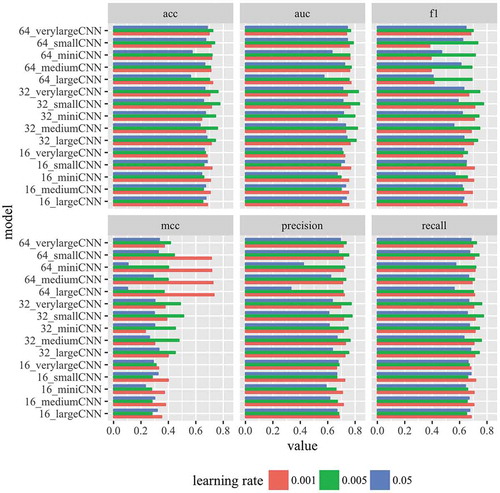
Because of successful application of convolutional neural network (CNN) models to predict genome wide transcription factor binding sites, we first tested if CNN models can also accurately predict lncRNA and DNA interaction sites. We tested different multi-layered CNN models with six different evaluation metrics (Fig. 2) by varying number of kernels and learning rate. We found that the performance of the CNN models depend on the learning rate as well the number of kernels. For all the six metrics, learning rate of 0.001 yielded the best performance in the models that have 16 kernels in the CNN layer (Fig. 2). However, the models that have 32 kernels in the CNN layers performed the best with learning rate of 0.005 in all the six different metrics (Fig. 2). The models with 62 kernels in the CNN layer performed best with learning rate 0.005 in general except when the metric MCC is used (Fig. 2). In general, the learning rate of 0.005 performed the best across the six different metrics tested. These observations indicate that different values of hyper parameters should be tested when evaluating different deep learning models. Focusing on one single value of hyper-parameter might lead to wrong conclusions.

Figure 2. Performance of CNN models. Performance of 15 different CNN models are shown for six different evaluation metrics. Three learning rates were tested. See specifications of the models in Table 2.

Deep learning accurately predicts genome-wide lncRNA binding sites

The simplest version of CNN model with one CNN layer is very similar to deepbind model [13] for transcription factor binding sites (Table 2). The simplest CNN model (16_miniCNN) contained only one CNN layer with 16 kernels (Table 2). It performed moderately well with mean area under curve or mean AUC = 0.75) (Fig. 2). Based on AUC, the performance improved by increasing the number of kernels to 32 (32_miniCNN: mean AUC = 0.80). However, AUC didn’t improved with 64 kernels (64_ miniCNN: mean AUC = 0.76). Similar performance trend was also observed with this single layer CNN model for accuracy, precision, f1 score and recall; where choice of 32 kernels performed the best (Fig. 2) except for MCC in which choice of 64 kernels was the best (Fig. 2). In the context of DNA sequences, the kernels or filters in the first CNN layer indicate short motifs or sequences that discriminate the positive and negative cases. Here, a single CNN layer with 32 kernels was able to achieve a mean auc and accuracy of 0.80 and 75%, respectively (Fig. 2). Similar to how DNA binding by transcription factors is governed by sequence motifs, the binding of lncRNAs on the DNA is likely dictated by short sequence patterns on the DNA. The increase in the performance with 32 kernels from 16 kernels indicates existence of multiple sequence patterns and variations within the same sequence pattern.

We also explored if higher order relationships between the short sequence patterns contribute to lncRNA binding. Since a single CNN layer can’t capture such kind of interactions, we tested multi-layered CNN models containing two (smallCNN), three (mediumCNN), four (largeCNN) and 7 layers (verylargeCNN) (Table 2). Similar to miniCNN, we tested three choices of number of kernels (16, 32, and 64) on each of these multi-layered CNN models (Table 2). Interestingly, adding one additional layer to miniCNN improved the ability to differentiate between lncRNA binding and non-binding sequences (Fig. 2). 16_smallCNN (mean AUC = 0.77), 32_smallCNN (mean AUC = 0.83), 64_smallCNN (mean AUC = 0.82), performed better than their corresponding models with a single layer (Fig. 2). This means higher order relationships between the sequence patterns in the ChIRP-Seq peaks contribute to lncRNA binding to DNA. Using the other five metrics showed also showed that two-layered smallCNN model performed better (Fig. 2). Interestingly, adding more additional CNN layers (mediumCNN, largeCNN, and verylargeCNN) didn’t improve any of the five metrics (AUC, accuracy, f1 score, precision, and recall) compared to 32_smallCNN (Fig. 2). When MCC metric is used, 64_largeCNN model with 4 CNN layers performed slightly better than two layered 32_smallCNN model (Fig. 2).

In summary, a model with only two CNN layers with 32 kernels in each CNN layer performed the best based on the six metrics evaluated compared more complex models. Increasing the number of kernels to 64 or increasing the number of CNN layers didn’t improve the performance.

CNN model performs better than feature-based models and sequence-based models

The above CNN models capture local sequence patterns and their interactions between them but doesn’t really test if the entire length of lncRNA binding sequences is important. It’s possible that there are long range interactions between sequence patterns across DNA ChIRP-Seq peaks that contribute to the binding of lncRNAs. To explore this possibility, we generated deep learning models with recurrent long short-term memory layer (LSTM) (Fig. 1). RNN or LSTM layer in deep learning has the ability to capture long term dependencies in data in the form of a sequence. We generated three RNN models; each model having one single bidirectional LSTM layer with varying LSTM hidden units: 5, 15, and 30 in 5_smallRNN, 15_smallRNN, and 30_smallRNN, respectively (Table 2). The three LSTM models performed more worse compared to the best CNN model. 5_smallRNN, 15_smallRNN, and 30_smallRNN achieving mean AUCs of 0.58, 0.63, and 0.64, respectively. These poor results seem to be independent of the complexity of the LSTM models indicating no relationship between the size of the LSTM on the model performance. The results indicate that long range dependencies along the DNA sequence is not necessary for the binding of lncRNAs.

To check if deep learning models are really necessary for this problem, we also tested three feature-based traditional models: support vector machines (svm), logistic regression, and random forest on the data set (Table 3). We used the frequency count of all possible 4-mers in the sequences as features. By tuning appropriate parameters under each of these models, we extracted the best model, which gave the highest value for the metric of interest. Among these three, svm performed the best (Table 3) in terms of accuracy (69%), area under the curve (0.742); logistic regression performed best in terms of MCC (0.387), precision (0.700), recall (0.694), and f1 score (0.693). However, all of these three models roughly performed at similar levels; but yielded at least 10% lower than the best deep learning model (Table 3). This indicates that deep learning models predicts the lncRNA binding sites at a better rate compared to traditional models.

Table 3. Performance of feature-based models. Three feature-based models were tested using 6 evaluation metrics.

Model	AUC	Accuracy	MCC	Precision	Recall	F1
Support vector machines (svm)	0.74	68.66%	0.37	0.69	0.69	0.69
Random forest	0.73	67.24%	0.34	0.66	0.68	0.67
Logistic regression	0.73	67.35%	0.39	0.70	0.69	0.69

Triplex forming domains of lncRNAs

There has been some indication that lncRNA harbors triplex forming domains (TFDs) that interact with double stranded DNA via RNA-DNA triplex formation [17]. If this is true, we can decipher the TFDs within the lncRNAs by matching (using triplex forming rules) the short patterns or motifs ‘learned’ by a CNN model within the ChIRP-Seq binding sites to specific portions of the lncRNA.

Out of all CNN models, we found that 32_smallCNN performed significantly better than all the other models. For this reason, the 32_smallCNN models (which achieved the best performance) representing 13 lncRNA binding profiles were applied to their corresponding test sequences (only the positive cases of lncRNA binding). Here, convolution on the positive test sequences were performed using the kernels in the first CNN layer and the subsequences in each test sequence which yielded the maximum positive signal were extracted. These subsequences represent the sequence ‘motif’ or pattern that best match the kernels in first CNN layer in the 32_smallCNN models.

If the lncRNA binding is primarily dictated by triplex formation, lncRNAs should form triplex structures with these extracted subsequences. We used Triplexator [18] to test if lncRNAs can form triplex structures with these subsequences. With an allowed maximum of 3 mismatches, the lncRNAs formed triplex structures with a subset of the extracted subsequences representing 82% of the kernels (26 out of 32). This indicates that majority of the lncRNA binding sites are indeed triplex forming instances.

To obtain the TFDs of each lncRNA, we first extracted regions in the lncRNA which formed triplex structures (predicted via Triplexator) with the kernel matching subsequences as mentioned above. Then, we merged any regions in the lncRNA which are at the most 5 bp apart to obtain its triplex forming loci or domains. Shorter lncRNAs such as HOTAIR, ROX2, TERC etc. have fewer triplex forming domains (7, 1, and 4, respectively) compared to other longer lncRNAs such as TUG1 isoforms (Table 4; NR_002321.2, NR_002322.2, and NR_110490.1), and MEG3 isoforms (Table 4; NR_003633.3, NR_027651.2, and NR_027652.1).

Table 4. Triplex forming domains (TFDs) of lncRNAs. (A) Table indicates the number of triplex forming domains/oligos (TFDs) in lncRNAs. Isoforms are separated for lncRNAs with multiple isoforms. (B) Table indicates locations and sequence of triplex forming domains for two example lncRNAs: Human HOTAIR, and mouse MEG3 isoform NR_027652.1. Bolded TFDs have been experimentally validated by previous studies.

A
lncRNA		Triplex forming domain count
Hotair		7
Rox2		1
Terc		4
DACOR1		30
lincHSC2		5
Hotchon (Limb)		14
Hotchon (Glial)		13
RMRP		1
Tug1 (NR_002321.2)		64
Tug1 (NR_002322.2)		95
Tug1 (NR_110490.1)		67
EC7		2
MEG3 (NR_003633.3)		114
MEG3 (NR_027651.2)		112
MEG3 (NR_027652.1)		11
Lin28		15
Panct1		65
B
LncRNA	Starting	Ending	Sequence
Hotair	422	436	GAGAGGAAGGAGGG
	669	683	AGAGGAGGGAAGAG
	800	816	TGTATTTTTATTTTTT
	836	853	ATGAGGAAAAGGGAAAA
	1388	1402	GTGTGTTTTGTTGG
	1482	1494	GGGGTTGTGTAG
	2009	2025	AAGAACAGAAAAAAAA
NR_027652.1 (Meg3)	197	209	CCTCTACCTCCT
	650	675	GTGGGTGGGGTGGGGTGGGGTGCTT
	710	734	CATGTCCCCTCCCCCTCCTCCACC
	758	770	GGGGTAGTGGGG
	788	803	TAGGGTTGTTGTGAG
	974	989	AGGTGGGAAAGAGAA
	1091	1115	TCGCTGCTTTCCTTCCTCACCTCC
	1281	1293	TTTGCTGTTGTG
	1360	1373	GAAGAAAAGAAGA
	1742	1760	TTGGGGGGGTGGGAGAAA
	1822	1836	GGGCTGTTGTGAGG

Three lncRNAs HOTAIR, MEG3, and TUG1 have been studied in the context of triplex structures formation. One triplex forming domain positioned at 649–708 in HOTAIR, which has been experimentally verified [5] as a triplex forming domain was one of the 9 domains detected by our method (Table 4). One triplex forming domain located in the extreme c-terminus in the shortest mouse MEG3 isoform NR_027652.1 (Table 4) was experimentally verified to form triplex structures with DNA [19]. For this particular isoform, our method detected 12 triplex forming domains, out which one (Table 4; positioned at 1822–1836) matched the experimentally verified domain [20]. LncRNA TUG1 has been shown to form triplex structures [7], but the domains have not been experimentally verified yet. For TUG1, we detected 38, 59, and 41 domains in its three isoforms (Table 4). This indicates that our method has uncovered experimentally validated triplex forming domains in lncRNAs.

Next, we tested the triplex structure forming ability of TFDs in lncRNAs which have not been reported nor experimentally validated. For this, we picked one TFD at nucleotide 836–851 coordinates of HOTAIR sequence and one TFD at nucleotide 35–50 coordinates of TUG1 sequence (Fig. 3A). Triplex formation of the HOTAIR and TUG1 TFDs were tested with selected double stranded DNA sites next to genes HOXD3 and PPARGC1A, respectively (Figs. 3C–F). Electrophoretic mobility shift assays support triple helix formation of these TFDs with their corresponding DNA sequences selected from ChIRP-Seq peaks (Figs. 3C–F). A corresponding control shows that triplex formation doesn’t occur between the double stranded DNA and the control RNA sequence (Figs. 3C–F). Besides, the detected signal of the triplex structure formation increased with the amount of RNA used (Figs. 3C–F). These EMSA assays support the notion that HOTAIR and TUG1 form triplex structures with the selected targets via triplex domains which have not been reported before. In general, it provides some experimental validation to our approach of obtaining the triplex forming domains of lncRNAs using a trained deep learning model.

Figure 3. Electrophoretic mobility shift assays support triple helix formation. Triple helix formation between (A) HOTAIR novel TFD and HOXD3 and (B) TUG1 novel TFD and PPARGC1A, which were considered for in vitro validation. (C and D) Electrophoretic mobility shift assay of predicted binding domains (HOTAIR and TUG1). Complementary oligodeoxynucleotides were preincubated to form double stranded DNA and then incubated with either specific RNA of predicted triplex binding in HOTAIR (C) and TUG1 (D), or non-specific control RNA. RNA was applied in 25-fold or 50-fold excess; 1.1 equivalents were used of the pyrimidine-rich DNA strand to reduce the possibility of DNA:DNA-DNA triplex formation. A mobility shift that indicates triplex formation was only observed with the specific sequences of HOTAIR and TUG1 TFDs. Triplex formation increased wth the increased in concentrations of RNAs: HOTAIR (E) and TUG1 (F).

Discussion

We show that deep learning models can accurately predict genome-wide lncRNA binding peaks uncovered by ChIPR-Seq peaks. Majority of the subsequences within the peaks representing the kernels in the first CNN layer act as host for triplex structure formation by lncRNAs. The number of triplex forming domains or oligos (TFDs) within lncRNAs vary and have different sequence patterns. We experimentally verify two TFDs of lncRNAs HOTAIR and TUG1 predicted by our method (but previously unreported) using Electrophoretic mobility shift assays. Our results show that RNA-DNA triplex formation is one mechanism used at genome-wide level by lncRNAs to exert their functions.

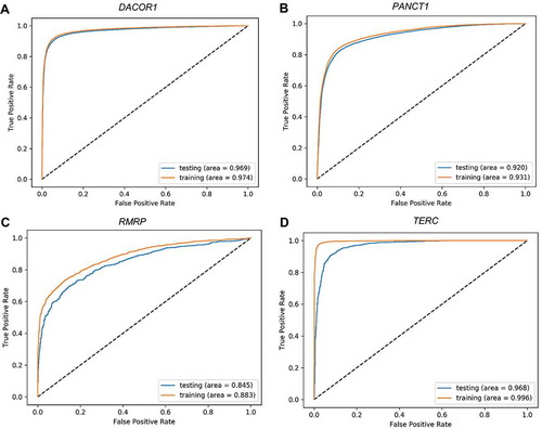
In this paper, we explore different architecture in deep learning models. The variation in the performance among the different architecture indicates that one needs to explore different architecture when it comes to developing deep learning models in genomics. However, one type of architecture seemed to perform consistently well across different ChIRP-Seq peaks of different lncRNAs. Small size of training set leads to overfitting and poor performance on the testing set in deep learning models. We found that some lncRNAs don’t have a lot of binding sites, hence were not appropriate for training deep learning models. For such lncRNAs, with the technique of data augmentation, we created new training sequences by shifting the original peaks to the left or right with a random amount. This resonates with proven data augmentation method of rotating images by a random degree in traditional image classification using deep learning models. Since the testing set should reflect an accurate ‘future’ sequences of unknown class label, we only applied data augmentation to the training set and not the testing set. To prevent overfitting, we used some proven techniques for training deep learning models. We used the drop out technique and batch normalization. Drop out is a technique of randomly removing neurons from hidden layer during training process making the trained model to act like an ensemble of different models which eventually outperforms the corresponding model without dropout. Batch normalization normalizes input data to a layer on a mini-batch basis which eventually improves the optimization process. We also imposed an ‘an early stopping’ in the optimization process of the models to prevent any overfitting. The optimization process was stopped when the value of the loss function on the validation set didn’t decrease for 11 consecutive steps or epochs. Manual inspection of the ROC plots (Fig. 4) show resemblance between the training and testing set. In deep learning models, pooling layer usually follows a convolution layer. But, there are different pooling techniques such as max, average, and L2-norm, which can be applied at the local or global level. For genomic signals, global-max pooling has shown to be more appropriate across multiple cases [16]. Because of this reason, we used global-max pooling in the CNN models.

Figure 4. Receiver Operating Characteristic (ROC) plots for training and testing sets. Four representative ROC plots for the best deep learning model representing four lncRNAs: TUG1 (A), HOTAIR (B), HOTCHON (C), and DACOR1 (D). Area under the curve for testing and training sets are shown for each plot.

Here, we conclude that short sequence patterns in ChIRP-Seq peaks that dictate lncRNA binding act as host for triplex structure formation by lncRNAs. The best model had 2 convolutional layers with pooling layers, drop out and batch normalization. Due to non-linear nature of the model as use of drop out and batch normalization techniques, we did not focus on measuring the importance of each kernel in the first CNN layer of the model. We focussed on finding the TFDs of lncRNAs instead of motifs that occurred in ChIRP-Seq peaks. Extracting the TFDs from the lncRNAs keeps the analysis lncRNAs-focused instead of ChIRP-Seq focused. One possible future direction of our work is to achieve a deeper biological interpretation of the TFDs of the lncRNAs. LncRNAs seem to have multiple TFDs. Do the TFDs have the same effect on gene regulation? For example, one TFD of a lncRNA may interact with a set of DNA sites to activate genes; and another TFD of the same lncRNA may repress a different group of genes. Another possible extension of this work is quantifying the importance of TFDs in lncRNAs.

In this paper, we extracted sequences of equal length centered at the midpoint of the peaks. In doing so, the input sequences to the models were of the same length. However, the input training data or matrix can be modified in such a way to handle sequences of different length. Let’s assume that M is the length of the longest sequence from the set of all peaks. If the length of a particular sequence (L) is less than M, M-L number of ‘N’ bases can be padded at th sequence to make the length of the sequence equals M. The raw nucleotide characters (A, C, G, T) in the sequence can be converted into a one hot encoding (a binary vector with the matching character entry being a 1 and the rest as 0s). The character ‘N’ can be encoded as a vector of 0 entries. If the preprocessing step is done in this manner, the models can be applied to sequences of different length.

Disclosure statement

No potential conflict of interest was reported by the authors.

Additional information

Funding

This work was supported by the Department of Defense [68847MAREP/W911NF1610480 to BS]; American Heart Association [181PA34170360] to YL and BS .

References

- Li Y, Syed J, Sugiyama H. RNA-DNA triplex formation by long noncoding RNAs. Cell Chem Biol. 2016;23:1325–1333.
- Grote P, Herrmann BG. The long non-coding RNA Fendrr links epigenetic control mechanisms to gene regulatory networks in mammalian embryogenesis. RNA Biol. 2013;10:1579–1585.
- Xue Z, Hennelly S, Doyle B, et al. A G-Rich Motif in the lncRNA braveheart interacts with a zinc-finger transcription factor to specify the cardiovascular lineage. Mol Cell. 2016;64:37–50.
- Engreitz JM, Ollikainen N, Guttman M. Long non-coding RNAs: spatial amplifiers that control nuclear structure and gene expression. Nat Rev Mol Cell Biol. 2016;17:756–770.
- Kalwa, M., Hänzelmann S, Otto S, et al. The lncRNA HOTAIR impacts on mesenchymal stem cells via triple helix formation. Nucleic Acids Res. 2016;44:10631–10643. DOI:10.1093/nar/gkw802.
- Mondal T, Subhash S, Vaid R, et al. MEG3 long noncoding RNA regulates the TGF-β pathway genes through formation of RNA-DNA triplex structures. Nat Commun. 2015;6.
- Long J, Badal SS, Ye Z, et al. Long noncoding RNA Tug1 regulates mitochondrial bioenergetics in diabetic nephropathy. J Clin Invest. 2016;126:4205–4218.
- Chu C, Qu K, Zhong FL, et al. Genomic maps of long noncoding RNA occupancy reveal principles of RNA-chromatin interactions. Mol Cell. 2011;44:667–678.
- Carlson HL, Quinn JJ, Yang YW, et al. LncRNA-HIT functions as an epigenetic regulator of chondrogenesis through its recruitment of p100/CBP complexes. PLoS Genet. 2015;11:e1005680.
- Terashima M, Tange S, Ishimura A, et al. MEG3 long noncoding RNA contributes to the epigenetic regulation of epithelial-mesenchymal transition in lung cancer cell lines. J Biol Chem. 2017;292:82–99.
- Krizhevsky A, Sutskever I, Hinton GE. ImageNet classification with deep convolutional neural networks. Adv Neural Inf Process Syst. 2012;6:1–9.
- Salakhutdinov R. Learning deep generative models. Annu Rev Stat Appl. 2015;2:361–385.
- Alipanahi B, Delong A, Weirauch MT, et al. Predicting the sequence specificities of DNA- and RNA-binding proteins by deep learning. Nat Biotechnol. 2015;33:831–838.
- Zhou J, Troyanskaya OG. Predicting effects of noncoding variants with deep learning-based sequence model. Nat Methods. 2015;12:931–934.
- Pan X, Shen H-B. Predicting RNA–protein binding sites and motifs through combining local and global deep convolutional neural networks. Bioinformatics. 2018;34:3427–3436.
- Zeng H, Edwards MD, Liu G, et al. Convolutional neural network architectures for predicting DNA-protein binding. Bioinformatics. 2016;32:i121–i127.
- Soibam B. Super-lncRNAs: identification of lncRNAs that target super-enhancers via RNA:DNA:DNA triplex formation. RNA. 2017;23:1729–1742.
- Buske FA, Bauer DC, Mattick JS, et al. Triplexator: detecting nucleic acid triple helices in genomic and transcriptomic data. Genome Res. 2012;22:1372–1381.
- Modali SD, Parekh VI, Kebebew E, et al. Epigenetic regulation of the lncRNA MEG3 and its target c-MET in pancreatic neuroendocrine tumors. Mol Endocrinol. 2015;29:224–237.
- Zhang L, Yang Z, Trottier J, et al. Long noncoding RNA MEG3 induces cholestatic liver injury by interaction with PTBP1 to facilitate shp mRNA decay. Hepatology. 2017;65:604–615.